Investigating the Effects of Altitude and Flap Setting on ...

Investigating the Effects of Altitude and Flap Setting on the Specific Excess Power

of a PA-28-161 Piper Warrior

By

Tjimon Meric Louisy

A thesis submitted to the College of Engineering and Science of

Florida Institute of Technology

In partial fulfillment of the requirements

For the degree of

Master of Science

in

Flight Test Engineering

Melbourne, Florida

December 2019

We the undersigned committee hereby approve the attached thesis, “Investigating the

Effects of Altitude and Flap Setting on the Specific Excess Power of a PA-28-161

Piper Warrior”, by Tjimon Meric Louisy.

_________________________________________________

Brian A. Kish, Ph.D.

Assistant Professor

Aerospace, Physics and Space Sciences

Major Advisor

_________________________________________________

Isaac Silver, Ph.D.

Associate Professor

College of Aeronautics

_________________________________________________

Ralph Kimberlin, Dr. Ing

Professor


_________________________________________________

Daniel Batcheldor

Professor and Department Head


iii

Abstract

Investigating the Effects of Altitude and Flap Configuration on the

Specific Excess Power of a PA-28-161 Piper Warrior

Tjimon Meric Louisy

Advisor: Brian A. Kish, Ph.D.

The high number of General Aviation (GA) accidents attributed to Loss of Control

suggests that GA pilots are lacking low speed awareness and are unable to

appropriately recognize when the aircraft is in a low energy state. There is, therefore,

an urgent need for the development of an energy management system which is

applicable to GA aircraft that can alert the pilot in situations of low energy conditions

and recommends to the pilot the appropriate corrective action to restore conditions to

a safe energy state. This will require the development of an algorithm that governs this

energy management system that considers a comprehensive understanding of the

performance capabilities of GA aircraft, particularly the ability of the aircraft to

progress from one energy state to another. Given that low energy conditions are the

primary concern, the aircraft’s ability to progress from a low energy state to a higher

energy state, or the aircraft’s specific excess power (Ps), will be the parameter of most

interest.

The focus of this research study was the testing of a PA-28-161 Piper Warrior to

develop an understanding of the effects of altitude and flap configuration on the ability

of the aircraft to change its energy state. Level accelerations and level decelerations

iv

were performed and used to determine the Ps for the aircraft at various altitudes and

configurations. The objectives of the test program were to generate Ps curves for each

altitude and configuration, compare the curves obtained, and determine trends that

could help model the Ps of the aircraft under any operating conditions.

The results of the test program showed that there was an inverse relationship between

specific excess power and altitude for both the clean-flap and full flaps configurations.

The best climb speed for the aircraft was approximately 79 KIAS in the clean

configuration and 62 KIAS in the full flaps configuration. Furthermore, extending the

flaps resulted in a significant decrease in the maximum specific excess power of the

aircraft, with the maximum specific excess power in the full flaps configuration being

approximately 200 ft/min less than the maximum specific excess power in the clean

configuration for all altitudes investigated. The best glide speed was observed to be 75

KIAS in the clean configuration.

The data collected and trends observed will be valuable in the development of an

algorithm for a GA energy management system. Further investigation into the Ps with

the flaps deployed and comparison between the trends observed on the PA-28-161

with other common GA aircraft parameters will also be required.

v

Table of Contents Abstract .............................................................................................................................. iii

Table of Contents ................................................................................................................. v

List of Figures ..................................................................................................................... vii

List of Tables ....................................................................................................................... xi

List of Abbreviations and Symbols ...................................................................................... xii

Acknowledgements........................................................................................................... xiv

Dedication ........................................................................................................................ xvi

Section 1 Introduction......................................................................................................... 1

Section 2 Test Methods and Materials ...............................................................................14

2.1 Test Aircraft .............................................................................................................14

2.2 Instrumentation .......................................................................................................15

2.3 Flight Log ..................................................................................................................16

2.4 Flight Test Locations and Crew .................................................................................17

Section 3 Data Reduction Methods ....................................................................................18

3.1 Data Requirements...................................................................................................18

3.2 Test Procedures........................................................................................................19

3.3 Data Reduction.........................................................................................................21

Section 4 Results ................................................................................................................32

4.1 Ps Plots (𝒂𝒔𝒔𝒖𝒎𝒆 𝒅𝒉/𝒅𝒕 = 𝟎) .................................................................................32

vi

4.1.1 Steady-Level Accelerations ................................................................................32

4.1.2 Steady-Level Decelerations ................................................................................51

4.2 Comparison to POH ..................................................................................................58

4.3 Ps Plots (𝒅𝒉/𝒅𝒕) component included ......................................................................59

4.3.1 Steady-Level Accelerations ................................................................................60

4.3.2 Steady-Level Decelerations ................................................................................64

Section 5 Conclusions and Future Work .............................................................................68

5.1 Conclusions ..............................................................................................................68

5.2 Recommendations and Future Works .......................................................................73

References .........................................................................................................................76

Appendix A: Flight Test Data ..............................................................................................78

Appendix B: Supplementary Graphs ...................................................................................98

vii

List of Figures

Figure 1: Loss of control in flight accidents and fatalities in GA 2011-2015 [2] ..................... 2

Figure 2 Fatal accidents per aircraft upset event types 2011-2015 [2] ................................. 3

Figure 3: Altitude-velocity diagram showing lines of constant specific Energy (Es) [5] .......... 7

Figure 4: Sample Ps Curves and Resulting Constant Ps Contours [9] ....................................10

Figure 5: Specific Total and Modified Total Energy Error Rate during approach [10] ...........12

Figure 6 PA-28-161 Piper Warrior – N618FT .......................................................................14

Figure 7: Test Locations [12] ..............................................................................................17

Figure 8: CAS vs Time (First 15s) .........................................................................................23

Figure 9: CAS vs Time (16s Onwards) ..................................................................................24

Figure 10: Pressure Altitude vs Time ..................................................................................25

Figure 11: Modeling Pressure Altitude vs Time ...................................................................27

Figure 12: Ps vs CAS Level-Acceleration ..............................................................................30

Figure 13: Ps vs CAS Level-Acceleration (𝒅𝒉/𝒅𝒕 ≠ 𝟎) ........................................................30

Figure 14: : Ps vs CAS Level-Deceleration ............................................................................31

Figure 15: Ps vs CAS for Clean Configuration Level-Accelerations ........................................32

Figure 16: : Ps vs CAS for Full Flaps Configuration Level-Accelerations ................................34

Figure 17: : Relationships between Ps and Altitude .............................................................35

Figure 18: Relationships between Vh and Altitude ..............................................................36

Figure 19: Relationships between Vy and Altitude ...............................................................37

Figure 20: Equation-derived Ps curves.................................................................................39

viii

Figure 21: Ps curves for Level-Accelerations at 1300 feet ....................................................41




Figure 25: Equation-derived Ps curves for Full Flaps Configuration......................................49

Figure 26: Ps Curves for Clean Configuration Level-Decelerations .......................................51

Figure 27: Ps Curves for Full Flaps Configuration Level-Decelerations .................................52

Figure 28: Ps Curves for Level-Decelerations at 1300 feet ...................................................53




Figure 32: Ps Curves for Clean Configuration Level-Accelerations (𝒅𝒉/𝒅𝒕 ≠ 𝟎) ..................60

Figure 33: Ps Curves for Full Flaps Configuration Level-Accelerations (𝒅𝒉𝒅𝒕 ≠ 𝟎) ..............61

Figure 34: Ps Curves for Level-Accelerations at 1300 feet (𝒅𝒉/𝒅𝒕 ≠ 𝟎) ..............................61




Figure 38: Ps Curves for Clean Configuration Level-Decelerations (𝒅𝒉/𝒅𝒕 ≠ 𝟎) .................64

Figure 39: Ps Curves for Full Flaps Configuration Level-Decelerations (𝒅𝒉𝒅𝒕 ≠ 𝟎) ..............65

Figure 40: Ps Curves for Level-Decelerations at 1300 feet (𝒅𝒉/𝒅𝒕 ≠ 𝟎) .............................65




ix

Figure 44: CAS vs Time 1300 feet Clean Level-Acceleration (First 15s) ................................78

Figure 45: CAS vs Time 1300 feet Clean Level-Acceleration (16s to end of run) ...................78

Figure 46: Pressure Altitude vs Time 1300 feet Clean Level-Acceleration ............................79

Figure 47: CAS vs Time 1300 feet Clean Level-Deceleration ................................................79

Figure 48: Pressure Altitude vs Time 1300 feet Clean Level-Deceleration ...........................80

Figure 49: CAS vs Time 1300 feet Full Flaps Level-Acceleration (First 20s)...........................80

Figure 50: CAS vs Time 1300 feet Full Flaps Level-Acceleration (21s to end of run) .............81

Figure 51: Pressure Altitude vs Time 1300 feet Full Flaps Level-Acceleration ......................81

Figure 52: CAS vs Time 1300 feet Full Flaps Level-Deceleration ..........................................82

Figure 53: Pressure Altitude vs Time 1300 feet Full Flaps Level-Deceleration......................82














x
















Figure 82; CAS vs Time 7000 feet Full Flaps Level-Deceleration ..........................................97


Figure 84: Change in Vy due to Flap Extension [13] .............................................................98

Figure 85: Altitude Effect on Vy [14] ...................................................................................99

xi

List of Tables

Table 1: Fatal LOC Accidents from 2011 to 2015 in GA and Commercial Operations [8] ....... 8

Table 2: Flight Log ..............................................................................................................16

Table 3: Values to Produce Aircraft Specific Excess Power Curve in Clean Configuration .....38

Table 4: Max Ps Comparison between Clean Configuration and Full Flaps Configuration .....45

Table 5: VH Comparison between Clean Configuration and Full Flaps Configuration ...........46

Table 6: Vy Comparison between Clean Configuration and Full Flaps Configuration ............46

Table 7: Values to Produce Aircraft Specific Excess Power Curve for Full Flaps ...................49

Table 8: Comparison between POH Values and Measured Values ......................................58

xii

List of Abbreviations and Symbols

AFM Airplane Flight Manual

ASEL Airplane Single Engine Land

CAS Calibrated Airspeed

CFIT Controlled Flight Into Terrain

CFR Code of Federal Regulations

EASA European Aviation Safety Agency

ESP Electronic Stability & Protection

Es Specific Energy

FAA Federal Aviation Administration

FTE Flight Test Engineer

GA General Aviation

HP Horsepower

Hp Pressure Altitude

IATA International Air Transportation Association

IAS Indicated Airspeed

KCAS Knots Calibrated Airspeed

xiii

KIAS Knots Indicated Airspeed

LOC Loss of Control

LOC-I Loss of Control In-flight

NTSB National Transport Safety Board

OAT Outside Air Temperature

POH Pilot’s Operating Handbook

Ps Specific Excess Power

TAS True Airspeed

ROC Rate of Climb

SD Secure Digital

USP Underspeed Protection

VH Maximum Level Flight Speed

VY Best Rate of Climb Airspeed

xiv

Acknowledgements

First, I would like to thank God for the endless blessings that He has bestowed upon

me throughout my life, and especially during my academic career. Without His

continued grace, none of my accomplishments, including this thesis, would have been

possible. I am also particularly grateful to my entire family for their prayers, advice

and encouragement throughout my academic career, especially during my pursuit of a

college education.

I would like to extend my sincerest thanks to my thesis advisor, Dr. Brian Kish, for his

continual support throughout my coursework and his excellent counsel towards the

completion of my thesis research. His extensive experience and genius made

performing this research a great learning and extremely fulfilling experience. I was

given the liberty to perform most of the work on my own, but could always count on

his cerebration whenever I ran into difficulty. Indeed, this thesis would not have been

a possibility without him. Furthermore, I would like to express my gratitude for the

profound impact he has had on my academic and career path. Following the

completion of my undergraduate degree, I had a general idea of where I wanted to be

career wise but was uncertain of the path that I would need to take to get there. His

constant advice and willingness to work with me to define the most appropriate path

was a service far beyond measure and what was required of him as an academic advisor

and professor. As a result of this, I am now well poised to achieve the career goals that

I have set and look forward to an enjoyable journey in getting there.

xv

I would also like to thank Dr. Ralph Kimberlin for his constant impartment of

knowledge and experience which has significantly accelerated my growth in the area

of Flight Test. His extensive knowledge and his willingness to share has allowed me

to develop a knowledge base far advanced of someone of similar experience.

I would like to acknowledge Dr. Isaac Silver, who performed the flight tests that

provided the data for this thesis and graciously agreed to be a member of my thesis

committee. Though my interaction with Dr. Silver throughout my academic career was

limited, his willingness to share his vast wealth of knowledge and experience was quite

evident from the fortunate occasions on which I interacted with him.

xvi

Dedication

This thesis is dedicated to my parents, Trevor and Luvette Louisy, who have

continually supported me throughout my years of seeking a higher-level education and

pursuing a career as an engineer in the aviation industry. Their constant support, both

financial and prayerful encouragement and well-timed advice have spurred me along

my journey prior to and at Florida Tech and will continue to motivate me as I continue

along my life path.

1

Section 1 Introduction

A Loss of Control (LOC) accident involves an unintended departure of an aircraft from

controlled flight and is the major cause of aircraft fatalities in general aviation (GA)

according to Federal Aviation Administration (FAA), with there being one fatal

accident involving Loss of Control every four days [1]. Though Loss of control

accidents in GA are currently on a downward trend, the number of accidents and

fatalities due to LOC (or loss of control – in flight [LOC-I] as it is referred to in many

EASA documents) are still alarmingly high, as displayed in Figure 1 below. Over the

five-year period analyzed, LOC accounted for an average of 39 fatal accidents and an

average of 66 fatalities each year; therefore, being the root cause for more than 80%

of the fatal accidents and fatalities recorded in Europe in that timeframe [2]. The

numbers in North America, though slightly better, are still cause for great concern.

The National Transportation Safety Board indicated that LOC played a role in more

than 40% of all single-engine, fixed-wing GA fatal accidents [3].

2

Figure 1: Loss of control in flight accidents and fatalities in GA 2011-2015 [2]

Though loss of control can occur during any phase of flight, statistics show that LOC

incidents are more frequent during the takeoff, approach, and landing phases of flight.

Over the same five-year period (2011-2015) analyzed, the EASA found that over 70%

of LOC accidents took place during those three aforementioned phases of flight, with

takeoff accounting for a little less than one third (31 %) of those accidents (Figure 2).

Additionally, Figure 2 shows that spin and stall were the two most common type of

aircraft upsets resulting from loss of control. Given that a spin must be preceded by an

aerodynamic stall, the two types can be combined into one category, therefore

accounting for more than 60% of aircraft upset events recorded in the five-year

timeframe.

3

Figure 2 Fatal accidents per aircraft upset event types 2011-2015 [2]

The takeoff, approach and landing phases of flight are known slow speed operations,

and pilots are trained to be extra diligent when monitoring airspeed during these phases

of flight. However, the data points to the contrary, indicating that pilots are losing

airspeed awareness, not recognizing the warning symbols of impending stall and

ultimately stalling the airplane during these low speed operations. The primary goal of

the pilot, especially during these low speed phases of flight, is to fly the aircraft. Yet

the trends displayed in Figure 2 point to the pilot getting distracted by auxiliary tasks,

losing low airspeed awareness and unable to recognize impending stall.

Stalling an aircraft is generally not “a nail in the coffin” moment as 14 CFR 23.2150

enforces aircraft to have controllable stall characteristics in all phases of flight and

therefore, not have the tendency to inadvertently depart from controlled flight [4].

However, the takeoff, approach and landing phases of flight are also low altitude

operations that take place within the traffic pattern (generally 1000 feet above ground

4

level), giving the pilot minimal time to correctly identify the upset and perform the

appropriate recovery procedure.

Furthermore, the combination of slow speed (low kinetic energy) and low altitude (low

potential energy) puts the aircraft at its lowest total energy during these phases of

flight, making the aircraft most susceptible to LOC during these phases. Pilot

awareness of the energy state of the airplane and proper energy management is,

therefore, critical to safely operate the aircraft during these phases of flight.

The total energy of an aircraft is the sum of the aircraft’s potential energy, a function

of the aircraft’s altitude in reference to the ground, and the aircraft’s kinetic energy, a

function of the aircraft’s velocity. The total energy is depicted mathematically in the

equation below:

𝐸 = 𝐸𝑝𝑜𝑡 + 𝐸𝑘𝑖𝑛 = 𝑚𝑔ℎ +1

2𝑚𝑉2 [1]

𝑊ℎ𝑒𝑟𝑒:

𝐸 = 𝑎𝑖𝑟𝑐𝑟𝑎𝑓𝑡′𝑠 𝑡𝑜𝑡𝑎𝑙 𝑚𝑒𝑐ℎ𝑎𝑛𝑖𝑐𝑎𝑙 𝑒𝑛𝑒𝑟𝑔𝑦

𝐸𝑝𝑜𝑡 = 𝑔𝑟𝑎𝑣𝑖𝑡𝑎𝑡𝑖𝑜𝑛𝑎𝑙 𝑝𝑜𝑡𝑒𝑛𝑖𝑎𝑙 𝑒𝑛𝑒𝑟𝑔𝑦 (𝑚𝑔ℎ)

𝐸𝑘𝑖𝑛 = 𝑘𝑖𝑛𝑒𝑡𝑖𝑐 𝑒𝑛𝑒𝑟𝑔𝑦 (1

2𝑚𝑉2)

𝑔 = 𝑔𝑟𝑎𝑣𝑖𝑡𝑎𝑡𝑖𝑜𝑛𝑎𝑙 𝑎𝑐𝑐𝑒𝑙𝑒𝑟𝑎𝑡𝑜𝑛

ℎ = 𝑎𝑖𝑟𝑐𝑟𝑎𝑓𝑡′𝑠𝑎𝑙𝑡𝑖𝑡𝑢𝑑𝑒 𝑎𝑏𝑜𝑣𝑒 𝑔𝑟𝑜𝑢𝑛𝑑 𝑟𝑒𝑓𝑒𝑟𝑒𝑛𝑐𝑒

𝑉 = 𝑎𝑖𝑟𝑐𝑟𝑎𝑓𝑡′𝑠 𝑣𝑒𝑙𝑜𝑐𝑖𝑡𝑦

5

The aircraft can be assumed to be a point-mass and the application of Newton’s second

law results in the following equation for the forces acting on the aircraft along its flight

path:

𝑇 − 𝐷 = 𝑊𝑠𝑖𝑛(𝛾) + 𝑚𝑎 [2]

𝑤ℎ𝑒𝑟𝑒:

𝑇 = 𝑡ℎ𝑟𝑢𝑠𝑡

𝐷 = 𝑑𝑟𝑎𝑔

𝑊 = 𝑎𝑖𝑟𝑐𝑟𝑎𝑓𝑡′𝑠 𝑤𝑒𝑖𝑔ℎ𝑡

𝛾 = 𝑓𝑙𝑖𝑔ℎ𝑡 𝑝𝑎𝑡ℎ 𝑎𝑛𝑔𝑙𝑒

𝑚 = 𝑎𝑖𝑟𝑐𝑟𝑎𝑓𝑡′𝑚𝑎𝑠𝑠

𝑎 = 𝑎𝑖𝑐𝑟𝑎𝑓𝑡′𝑠𝑎𝑐𝑐𝑒𝑙𝑒𝑟𝑎𝑡𝑖𝑜𝑛

From equation 2 above, it can be seen that when 𝛾 = 0 𝑎𝑛𝑑 𝑎 = 0, (𝑇 − 𝐷) = 0,

representing the steady-state equation for level, unaccelerated flight.

The law of conservation of energy states that energy can neither be created nor

destroyed – only converted from one form of energy to another [7]. In the case of level,

unaccelerated flight, the aircraft’s total mechanical energy will be constant. From

equation 1, the aircraft’s mass and gravitational acceleration are constant, indicating

that energy can be transferred from potential to kinetic solely by descending in altitude

in exchange for an increase in airspeed. This exchange of energy is depicted on Figure

3 as a move from point A to point B.

6

The transfer of energy, however, is not limited to within the system only, as the

conservation law also states that energy can be added to or removed from the energy

stored in an open system. In the case of an aircraft, energy is transferred to the system

(aircraft) via the engine thrust, while energy is transferred from the system (aircraft)

via drag. However, the law of conservation of energy cannot be violated, indicating

that there must be a balance between the net flow of energy transferred through the

system (energy transferred in minus energy transferred out) and the resultant change

in energy stored in the system illustrated by equation (3) below:

𝐸𝑇 − 𝐸𝐷 = ∆𝐸 [3]

𝑊ℎ𝑒𝑟𝑒:

𝐸𝑇 = 𝑒𝑛𝑒𝑟𝑔𝑦 𝑔𝑎𝑖𝑛𝑒𝑑 𝑡ℎ𝑟𝑜𝑢𝑔ℎ 𝑡ℎ𝑟𝑢𝑠𝑡

𝐸𝐷 = 𝑒𝑛𝑒𝑟𝑔𝑦 𝑙𝑜𝑠𝑠 𝑡ℎ𝑟𝑜𝑢𝑔ℎ 𝑑𝑟𝑎𝑔

∆𝐸 = 𝑐ℎ𝑎𝑛𝑔𝑒 𝑖𝑛 𝑡𝑜𝑡𝑎𝑙 𝑚𝑒𝑐ℎ𝑎𝑛𝑖𝑐𝑎𝑙 𝑒𝑛𝑒𝑟𝑔𝑦

From equation 3 above, it can be seen that ∆𝐸 will be positive if 𝐸𝑇 is greater than 𝐸𝐷 ,

resulting in excess energy, or vice-versa, resulting in deficit energy. Excess energy is

required for the aircraft to increase its total energy such as climbing to an altitude while

maintaining airspeed, and is depicted on Figure 3 as a move from point B to C.

However, excess energy is not a very useful parameter, as it only indicates that a

movement from point B to C is possible, but gives no indication how long it will take

the aircraft to reach energy state C. Taking the derivative of equation of 3 with respect

to time gives the rate of change of the airplane’s total mechanical energy (�̇�), or as it

is more commonly known as, the power as displayed in equation 4.

7

�̇� = �̇�𝑇 − �̇�𝐷 = 𝑚𝑔 (𝑑ℎ

𝑑𝑡) + 𝑚𝑉(

𝑑𝑣

𝑑𝑡) [4]

Similarly, if �̇�𝑇 is greater than �̇�𝐷 , the aircraft will possess excess power, not only

indicating that a move from point B to C in Figure 3 is possible, but also indicating

how long it would take the aircraft to reach that new energy state. Dividing equation

4 by weight (mg) gives the rate of change at which the airplane is able to change its

total mechanical energy per unit weight, a term known as specific excess power which

is presented in equation 5 below.

𝑃𝑠 =𝑑ℎ

𝑑𝑡+𝑉

𝑔(𝑑𝑣

𝑑𝑡) [5]

Figure 3: Altitude-velocity diagram showing lines of constant specific Energy

(Es) [5]

8

The number of loss of control accidents, though still an area for concern, are

significantly lower in commercial operations (Note: Commercial operations refer to

regularly scheduled ticketed passenger flights or cargo flights) when compared to

general aviation. The International Air Transport Association (IATA) indicated that

over a ten-year period (January 2009 to December 2018), 777 total commercial

aviation accidents were recorded, with 64 (approximately 8%) being classified as

LOC-I [8]. Table 1 below shows a comparison between the number of LOC accidents

recorded in GA and commercial operations over the same five-year period.

Table 1: Fatal LOC Accidents from 2011 to 2015 in GA and Commercial

Operations [8]

Number of

Fatal LOC

Accidents

2011 2012 2013 2014 2015

General

Aviation

50 48 33 31 28

Commercial

Operations

8 5 8 6 3

It is clear from Table 1 above that LOC accidents are extremely more prevalent in GA

operations when compared to commercial operations, almost 600% more frequent in

GA despite significantly more hours being flown in commercial operations.

Commercial operations owe their increased level of safety partly to better trained and

more experienced pilots, as well as having two pilots in the cockpit. However, the

increase in automation and implementation of systems such as autothrottles,

Underspeed Protection (USP) and Electronic Stability & Protection (ESP) contribute

to the impeccable safety of commercial aviation. These systems not only increase the

9

pilot’s awareness of the aircraft’s energy state, but also reduce pilot workload and in

emergency situations perform correct recovery procedures. The algorithms that govern

these systems are developed from an understanding of the energy characteristics of the

aircraft. Specific excess power is especially important to understand when designing

recovery procedures and setting the margins for safety mechanisms as it defines the

capability of the aircraft, indicating the limits at which the aircraft can safely operate

and governing the recovery procedure that is most appropriate to the situation. Figure

4 below displays specific excess power for various altitudes and how they are

combined to produce constant specific power contours.

10

Figure 4: Sample Ps Curves and Resulting Constant Ps Contours [9]

General aviation is still trying to catch up with the level of automation present in

commercial operations, with higher-end aircraft incorporating advanced autopilots

that include USP and ESP as well as autothrottles. However, most GA aircraft are old,

built in the last century, and are difficult to retrofit with some of these systems.

Additionally, the cost of most of these systems far exceed the cost of most of the

general aviation fleet, making these systems impractical. As a result, research has been

conducted into creating an energy management system that takes principles from these

11

proven systems in an attempt to improve the safety in GA. The system must be

relatively low cost, easily retrofitted onto aircraft and function off parameters already

recorded on the aircraft.

Energy metrics studies have been conducted in an attempt to begin developing an

algorithm that would govern this energy management system. Puranik et al (2017)

conducted an analysis in energy-based metrics in order to develop a reference for what

would define safe operation. Current operating conditions would then be compared to

this reference and based on the level of deviation from the reference would determine

the safety level of the current operation much like Figure 5 below. The top portion of

the figure displays the specific total energy during approach for all flights investigated,

and the shaded regions show the percentage of records within a certain region of

specific energy during the approach. The dashed line represents the average specific

total energy observed during the approach, and the solid line represents the individual

record being compared against the entire sample. The bottom portion of the graph

shows the modified total energy error rate, and essentially shows how far the current

record deviates from the established norm. Based on the data, one is able to establish

tolerance levels that ensures safe operation. Deviations beyond that tolerance (such as

between 2.0 and 1.5 nautical miles left) will trigger the algorithm to provide

appropriate corrective action to the pilot. However, the paucity of data available for

GA aircraft makes developing an accurate algorithm quite difficult. The research

presented in this thesis is intended to assist in alleviating this issue by generating Ps

curves that can be used in the development of this algorithm.

12

Figure 5: Specific Total and Modified Total Energy Error Rate during

approach [10]

This research is unique as it investigates the effects of altitude and flap configuration

on a Part 23 aircraft (PA-28-161). The PA-28-161 is a single-engine piston aircraft

certified to fly in the United States under CFR 14 Part 23. Single- engine piston aircraft

account for more than 80% of the GA fleet [11], making the results of this investigation

applicable to most of the GA fleet. Much of the research conducted into specific excess

power examines the aircraft in the flaps retracted configuration. As seen from FAA

and EASA statistics, the most critical phases of flight for LOC (takeoff, approach and

landing) almost always require flap operation. This investigation into the effects of

13

flap configuration will provide more operationally realistic data regarding specific

excess power during those critical phases, therefore greatly increasing the accuracy of

the algorithm. Additionally, this investigation examined relationships between altitude

and specific excess power, in order to generate trends for comparison. The ultimate

goal is to create a system that accurately models the energy of every aircraft it is

installed on. The analysis of the trends observed was conducted in an attempt to

develop a method that would generate an accurate algorithm, to avoid having to

perform extensive flight testing of every aircraft that the system is intended to go on.

Continued research into Ps in GA aviation is integral to reducing the amount of

accidents as a result of LOC, as shown by the “success” of commercial operations in

this accident category. Increased knowledge of performance metrics will allow for the

design of appropriate systems and measures that will help GA safety numbers

eventually match those of commercial operations, as it pertains to LOC.

14

Section 2 Test Methods and Materials

2.1 Test Aircraft

Figure 6 PA-28-161 Piper Warrior – N618FT

The test aircraft depicted in Figure 6 is PA-28-161 Piper Warrior with FAA

registration N618FT. The aircraft is owned and operated by the Flight Test

Engineering Department at Florida Institute of Technology. The Piper Warrior is a

single-engine light trainer with a maximum gross takeoff weight of 2440 pounds. The

aircraft is a low-wing, fixed landing gear, four-place aircraft powered by a normally

aspirated Lycoming O-320 engine producing a maximum of 160 hp. The aircraft has

a fixed pitch propeller and conventional flight controls, with full flaps setting

corresponding to 40 degrees of flap deflection. This aircraft was manufactured in 1985

and is equipped with the Garmin G5.

15

2.2 Instrumentation

All data requirements for the level acceleration and level deceleration tests were

parameters that are normally displayed to pilots; hence, no additional instrumentation

was required aside from the instruments/avionics suite already installed in the aircraft.

The only supplementary instrumentation used for data collection was an SD card.

The primary form of data collection used was the data recorded by G5 and stored on

the SD card installed inside it. Data displayed on the G5 were also collected on

handwritten flight test cards in the rare case that the SD card data were unreadable.

16

2.3 Flight Log

Table 2: Flight Log

Date Aircraft Crew Flight Time (hours)

03/25/2019 PA-28-161 Isaac Silver, Brian Kish 1.5

03/26/2019 PA-28-161 Isaac Silver, Tjimon

Louisy, Brian Kish

1.6

Table 2 above shows the log of test flights that were performed as a part of this

program. Instrument error resulted in no data being recorded on the flight performed

on 03/25/2019, requiring the crew to re-fly the test points on 03/26/2019.

17

2.4 Flight Test Locations and Crew

Figure 7: Test Locations [12]

All test flights were launched from the FIT Aviation facility at the Orlando Melbourne

International Airport (KMLB) in Melbourne, Florida. The tests were conducted in

areas to the east and southeast of the airport over the Atlantic Ocean.

The flight tests were conducted by a crew from the Florida Institute of Technology.

Isaac Silver was the pilot, and Tjimon Louisy and Brian Kish were the Flight Test

Engineers.

18

Section 3 Data Reduction Methods

3.1 Data Requirements

The test parameters required for the level acceleration and level deceleration tests

were:

(i) time

(ii) indicated airspeed

(iii) pressure altitude

(iv) outside air temperature.

The indicated airspeed was converted to calibrated airspeed using the airspeed

correction tables present in the PA-28-161 Warrior Pilot’s Operating Handbook

(POH). Additionally, the power-on stall speed and maximum level flight speed were

utilized for data reduction of the steady level accelerations.

19

3.2 Test Procedures

All tests were conducted over the Atlantic Ocean, in areas east and southeast of the

Orlando Melbourne International Airport (KMLB). The tests were conducted at 1300

feet, 3000 feet, 5000 feet and 7000 feet. The original test plan called out testing at

1000, 3000, 5000 and 7000 feet. However, conditions below 1300 feet on the day of

testing were deemed unfavorable for accurate data collection using the test procedures

that were to be employed. The test pilot was responsible for operating the aircraft and

performing the test point procedures, while the flight test engineer (FTE) recorded

pertinent data.

The level acceleration tests commenced with the pilot slowing the aircraft down to a

speed just above the power-on stall speed for the applicable configuration (clean or

full flaps) at an altitude just below the target altitude. The mixture was set to the full

rich position and the test pilot advanced the throttle to the full power position. The test

pilot allowed the aircraft to climb to the target altitude at the designated minimum

airspeed, and upon reaching the target altitude, the pilot levelled off and allowed the

aircraft to accelerate. The FTE recorded the GPS time (for reference when retrieving

data from the Garmin SD card) once the aircraft reached the target altitude and began

filling in the handwritten flight test cards. The pilot maintained altitude (within ±50

feet of the target altitude) and configuration until the airspeed stabilized. Once the

airspeed stabilized, the maximum level flight speed was recorded. The power-on stall

speeds were recorded during stall characteristics testing of the PA-28-161. These were

the lowest speeds achieved during testing in both configurations.

20

The level deceleration tests in the clean configuration commenced with the pilot

achieving maximum level flight speed at the target altitude. Once airspeed stabilized,

the FTE recorded the GPS time and the pilot retarded the throttle to idle power. For

the level deceleration tests in the full-flaps configuration, the pilot achieved the lower

of maximum flap extend speed or maximum level flight speed at the target altitude.

Once the airspeed stabilized, the FTE recorded the GPS time, and the pilot extended

the flaps to its maximum deflection and retarded the throttle to idle power. For both

the clean configuration and the full-flaps configuration, the pilot-maintained altitude

(within ±50 feet of the target altitude) and configuration until the plane decelerated to

the power-off stall speed, while the FTE filled in the handwritten flight test cards.

(Note: The tests were terminated at 1.1 times the applicable stall speed for the

configuration being tested at 1300 feet, to avoid stalling the aircraft at such a low

altitude).

21

3.3 Data Reduction

Flight test data were recorded using an SD card placed inside the Garmin Primary

Flight Display. The Garmin display recorded data at a speed of 1 hertz. This allowed

for the values for the necessary test parameters (altitude and airspeed) to be analyzed

in one-second increments. Given that the temperature would remain relatively constant

throughout the test run at the specified altitude, it was only recorded at the start of the

run using the OAT probe. After tabulating a spreadsheet with time, airspeed, and

altitude for each run, the following steps were performed to create Ps curves:

1. First, the airspeed corrections listed in the PA-28-161 Warrior Pilot’s

Operating Handbook (POH) were applied to the indicated airspeed (IAS)

values to obtain calibrated airspeed (CAS).

Example: 100 KIAS = 96 KCAS.

Note: The Garmin G5 was assumed to have zero instrument error.

2. The density ratio (σ) was then calculated using the equation 𝜎 =

(1−6.87535∗10−6∗ℎ𝑝)5.2561

(𝑇𝑎+273.15)

288.15

where Ta is the ambient temperature at altitude in

degrees Celsius.

Example:

𝜎 =(1 − 6.87535 ∗ 10−6 ∗ 3075𝑓𝑡)5.2561

(18 + 273.15)288.15

= 0.88456

22

3. The calibrated airspeed values were then converted from knots to ft/s.

Example:

100 𝑘𝑡𝑠 ∗ 6076.12 (

𝑓𝑡𝑛𝑚)

3600 (𝑠

ℎ𝑜𝑢𝑟)= 168.781 𝑓𝑡/𝑠

4. Microsoft Excel software was then used to plot the values of CAS in ft/s against

time and the trend line function was used to derive an appropriate curve fit. For

the steady-level accelerations, a piecewise function was used to accurately

represent the trends observed at the low-speed end of the plot. This was

required because of the unique behavior experienced at the low-speed end, due

to propeller efficiency and the complexity of the thrust curve associated with

propeller driven aircraft.

Example: Figures 8 and 9 show the plot of calibrated airspeed against time for

the PA-28-161 aircraft in the clean configuration during the level acceleration

run at 1300 feet. The equation of the curve fit to six decimal places is shown

below Figures 8 and 9. Figure 8 was solved for t = 10s as this piece-wise

function accurately modeled velocity versus time for the first 15 seconds of the

run, while Figure 9 was solved for t = 30s, as this piece-wise function

accurately modeled velocity versus time for t = 16 seconds and onwards for

the run.

23

Figure 8: CAS vs Time (First 15s)

𝑉𝑐 = −0.017493𝑡3 + 0.417240𝑡2 − 0.563237𝑡 + 104.456023

= −0.017493(103) + 0.417240(102) − 0.563237(10)+ 104.456023 = 123.05 𝑓𝑡/𝑠

y = -0.017493x3 + 0.417240x2 - 0.563237x + 104.456023

0

20

40

60

80

100

120

140

0 2 4 6 8 10 12 14 16

CA

S (f

t/s)

Time (s)

CAS vs Time for Steady-Level Acceleration in Clean Configuration

24

Figure 9: CAS vs Time (16s Onwards)

𝑉𝑐 = −0.012799𝑡2 + 2.046088𝑡 + 110.7742407

= −0.012799(302) + 2.046088(30) + 110.7742407= 160.64 𝑓𝑡/𝑠

5. The derivative of the curve fit was obtained and used to calculate the rate of

change of velocity (𝑑𝑣

𝑑𝑡) at each time step, or each fitted CAS value.

Example:

𝑑𝑉𝑐𝑑𝑡= −0.025598𝑡 + 2.046088 = −0.025598(30) + 2.046088 = 1.278

𝑓𝑡

𝑠2

y = -0.012799x2 + 2.046088x + 110.742407

0

50

100

150

200

250

0 10 20 30 40 50 60 70 80 90

CA

S (f

t/s)

Time (s)


25

6. The pressure altitude was then plotted against time and the trend line function

was used to derive an appropriate curve fit. The nature of the test required the

pilot to maintain altitude within ±50ft of the test condition altitude, resulting

in constant corrections and a plot that shows continuous increases and

decreases in altitudes. Note: The pressure altitude referenced to conduct

the test was that displayed on the altimeter set to 29.92. The pressure

altitude used in the data reduction was that recorded on the Garmin

Display. The Garmin Display had a positive offset when compared with

the altimeter. A 35 foot offset was noted at 1300 feet, a 70 foot offset was

noted at 3000 feet, a 90 foot was noted at 5000 feet, and a 120 foot offset

was noted at 7000 feet. An initial plot was created to attempt to model each

change in altitude over the entire run (see Figure 10 above) but became

2500

2600

2700

2800

2900

3000

3100

3200

3300

3400

3500

0 20 40 60 80 100 120

Hp

(ft

)

Time (s)

Hp vs Time for Steady-Level Acceleration in Clean Configuration

Figure 10: Pressure Altitude vs Time

26

extremely complex due to the number of changes and the limited ability of

Excel for this type of analysis. Additionally, the plots resulted in inaccurately

large rates of change due to the plot trying to encompass every single data

point. Therefore, a more simplistic polynomial curve that modeled the general

trend of the aircraft with reference to altitude (i.e. increasing, decreasing or

maintaining) as time progressed was chosen (see Figure 11 below). This model

tended to ignore the changes from point to point (one second increments) and

focused on the larger trends (generally changes in altitude over 5 seconds or

longer increments). This model appeared to be a better representation of what

the actual aircraft was experiencing, and the derivative of this model was used

to obtain more appropriate rates of change.

27

Figure 11: Modeling Pressure Altitude vs Time

𝐡 = −𝟎. 𝟎𝟎𝟎𝟎𝟎𝟐𝐭𝟒 + 𝟎. 𝟎𝟎𝟎𝟔𝟑𝟖𝒕𝟑 + 𝟎.𝟎𝟔𝟑𝟎𝟓𝟓𝒕𝟐 − 𝟐.𝟒𝟒𝟖𝟎𝟔𝟖𝐭+ 𝟑, 𝟎𝟒𝟏. 𝟒𝟕𝟑𝟗𝟕𝟗

𝑑ℎ

𝑑𝑡= −0.000008𝑡3 + 0.001914𝑡2 − 0.12611𝑡 + 2.448068

= −0.000008(0)3 + 0.001914(0)2 − 0.12611(0) + 2.448068

= 2.448068 𝑓𝑡

𝑠

7. True airspeed values were calculated using the known equation, 𝑉𝑇 =𝑉𝑐

√𝜎.

Example:

𝑉𝑇 =168.781 𝑓𝑡/𝑠

√0.88456= 179.4568 𝑓𝑡/𝑠

y = -0.000002x4 + 0.000638x3 - 0.063055x2 + 2.448068x + 3,041.473979

2500

2600

2700

2800

2900

3000

3100

3200

3300

3400

3500

0 20 40 60 80 100 120

Hp

(ft

)

Time (s)


28

8. The specific excess power values (Ps) were then calculated using values

obtained in previous steps. Two Ps values were calculated for each airspeed.

One using the conventional method that assumes the 𝑑ℎ

𝑑𝑡 component to be zero

and the other that includes the calculated 𝑑ℎ

𝑑𝑡 component. The Ps was calculated

in the units of ft/minute. The Ps equation is derived from the energy

equation, 𝐸 =1

2

𝑊

𝑔𝑣2 +𝑊ℎ. Dividing through by weight (W) gives 𝐸𝑠 =

1

2𝑔𝑣2 + ℎ. Taking the time derivative yields

𝑑

𝑑𝑡(𝐸𝑠) = 𝑃𝑠 =

𝑣

𝑔

𝑑𝑣

𝑑𝑡+𝑑ℎ

𝑑𝑡. The

equation used to calculate Ps without the 𝑑ℎ

𝑑𝑡 component was 𝑃𝑠 = (

𝑉𝑇

𝑔∗𝑑𝑣

𝑑𝑡) ∗

60. When the 𝑑ℎ

𝑑𝑡 component was included the equation became 𝑃𝑠 =

((𝑉𝑇

𝑔∗𝑑𝑣

𝑑𝑡) +

𝑑ℎ

𝑑𝑡) ∗ 60.

Examples:

𝑃𝑠 = (179.4568

𝑓𝑡𝑠

32.2 𝑓𝑡𝑠2

∗ 0.4589 𝑓𝑡

𝑠2) ∗ 60

𝑠

𝑚𝑖𝑛= 153.452

𝑓𝑡

𝑚𝑖𝑛

𝑃𝑠 =

(

(179.4568

𝑓𝑡𝑠

32.2 𝑓𝑡𝑠2

∗ 0.4589𝑓𝑡

𝑠2) + 0.2761

𝑓𝑡

𝑠

)

∗ 60 𝑠

𝑚𝑖𝑛= 170.018

𝑓𝑡

𝑚𝑖𝑛

9. Plots of Ps against KCAS were generated for every test run performed, with

and without the 𝑑ℎ

𝑑𝑡 components. The curves for the steady-level accelerations

29

were anchored on the low speed end by the power-on stall speed and on the

high-speed end by the maximum level flight speed as the aircraft has zero

excess power at those airspeeds. The curves for the steady-level decelerations

were not anchored on either end (low speed nor high speed), and only the data

collected during the run was plotted. Outlying points were not used in

calculating the Ps curve to allow for the most accurate result.

Example: Figure 12 shows the Ps plot for the PA-28-161 Warrior aircraft with the dh

dt

component assumed to be zero for the clean configuration acceleration at 1300 feet.

The power-on stalling speed is 56 KCAS and the maximum level flight speed VH is

119 KCAS. Figure 13 shows the Ps plot for the PA-28-161 Warrior aircraft with the

dh

dt component incorporated for the clean configuration acceleration at 3000 feet. The

power-on stalling speed is 56 KCAS and the maximum level flight speed VH is 114

KCAS. Figure 14 shows the Ps plot for the PA-28-161 Warrior aircraft with the dh

dt

component assumed to be zero for the clean configuration deceleration at 1300 feet.

The inclusion of the dh

dt component will not change the overall shape of the graphs, nor

the trends observed. However, the inclusion of the dh

dt component is to try to make the

absolute specific excess power values calculated for each airspeed more accurate. The

steady-level deceleration plots will be below the airspeed axis (x-axis), as there will

be a deficit in power (negative specific excess power).

30

Figure 12: Ps vs CAS Level-Acceleration

Figure 13: Ps vs CAS Level-Acceleration (𝒅𝒉

𝒅𝒕≠ 𝟎)

0

100

200

300

400

500

600

50.0 60.0 70.0 80.0 90.0 100.0 110.0 120.0 130.0

Ps

(ft/

min

)

CAS (KTS)

Specific Excess Power vs CAS for Steady-Level Acceleration in Clean Configuration at 1300 Feet

0

50

100

150

200

250

300

350

400

450

50.0 60.0 70.0 80.0 90.0 100.0 110.0 120.0 130.0

Ps

(ft/

min

)

CAS (kts)

Specific Excess Power vs CAS for Steady-Level Acceleration in Clean Configuration at 3000 feet

(with dh/dt component)

31

Figure 14: : Ps vs CAS Level-Deceleration

-1800

-1600

-1400

-1200

-1000

-800

-600

-400

-200

0

0.0 20.0 40.0 60.0 80.0 100.0 120.0 140.0

Ps

(ft/

min

)

CAS (kts)

Specific Excess Power vs CAS for Steady-Level Deceleration in Clean Configuration at 1300 feet

32

Section 4 Results

4.1 Ps Plots (𝒂𝒔𝒔𝒖𝒎𝒆 𝒅𝒉

𝒅𝒕= 𝟎)

The Ps plots analyzed for the steady-level accelerations and steady-level decelerations

are presented in Section 4.1.1 and Section 4.1.2 respectively.

4.1.1 Steady-Level Accelerations

Figure 15 below shows the specific excess power versus the calibrated airspeed in the

clean configuration for the four altitudes investigated.

Figure 15: Ps vs CAS for Clean Configuration Level-Accelerations

From the figure above it is observed that altitude had a negative effect on Ps, i.e. an

increase in altitude resulted in a lower specific excess power for all speeds. The

0

100

200

300

400

500

600

50.0 60.0 70.0 80.0 90.0 100.0 110.0 120.0 130.0

Ps

(ft/

min

)

CAS (KTS)

Specific Excess Power Vs CAS for Steady-Level Acceleration in Clean Configuration for Various Altitudes

1300 Feet 3000 Feet 5000 Feet 7000 Feet

33

reduction in specific excess power and the decrease in the maximum level flight speed

observed can be attributed to a deterioration in engine performance with altitude, both

in power and thrust available (via the propeller), for a normally aspirated piston

engine. Stall speed (KCAS), in accordance with the known theory, remained

unchanged with altitude. The slight variation noted was due to random error.

Additionally, Vy was approximately 79 KCAS for all altitudes, with a minor decrease

noted in Vy as altitude increased. This is well in line with the principle that a slight

decrease in Vy, in terms of CAS or IAS will occur as altitude increases, due to

movement in both the power available and power required curves. Increasing altitude

results in the power required curve moving upwards and shifting to the right. The

power available curve on the other hand, comes straight down, due to the deterioration

in engine performance with increased altitude. This results in Vy, in terms of TAS,

increasing (moving to the right) as seen in Figure 85 in Appendix B. However, this

increase in terms of TAS happens at a slower rate than the rate CAS or IAS fall behind

TAS as the aircraft climbs. The net result is a decrease in Vy, in terms of CAS or IAS.

34


full flaps configuration for the four altitudes investigated.

Figure 16: : Ps vs CAS for Full Flaps Configuration Level-Accelerations

From the figure above it is observed that an increase in altitude resulted in a reduction

in specific excess power. Deterioration in engine performance with altitude, both in

power and thrust available, for a normally aspirated piston engine is the main reason

for the reduction in specific excess power, and also accounts for the decrease in the

maximum level flight speed observed. Stall speed (KCAS), as expected from known

theory, remained unchanged with altitude (slight variation noted due to random error).

Vy was approximately 62 KCAS for all altitudes, with a minor decrease noted in Vy as

altitude increased. The minor decrease in Vy as altitude increased is also in line with

known theory, as discussed previously for the clean configuration (Figure 15).

0

50

100

150

200

250

300

350

400

40.0 50.0 60.0 70.0 80.0 90.0 100.0

Ps

(ft/

min

)

CAS (KTS)

Specific Excess Power Vs CAS for Steady-Level Acceleration with Full Flaps for Various Altitudes

1300 Feet 3000 Feet 5000 Feet 7000 Feet

35

Figure 17 below shows the maximum specific excess power versus pressure altitude

for the two configurations investigated.

Figure 17: : Relationships between Ps and Altitude

The figure above shows that there is an inverse linear relationship between altitude

and specific excess power for both configurations investigated. The figure also

indicates that altitude has a similar effect on specific excess power for both clean and

full flaps configuration, as displayed by the almost identical slopes of the graphs. The

figure above also shows that the aircraft has a sea-level specific excess power of

approximately 610 ft/min and 400 ft/min in the clean configuration and full flaps

configurations, respectively. Additionally, it is observed that the aircraft has an

absolute ceiling of approximately 12,800 feet and 8,500 feet in the clean configuration

y = -0.047379x + 608.070344R² = 0.942683

y = -0.047044x + 402.954017R² = 0.964446

0

100

200

300

400

500

600

0 1000 2000 3000 4000 5000 6000 7000 8000

Ps

(ft/

min

)

Pressure Altitude (ft)

Specific Excess Power Relationship with AltitudeClean Config Full Flaps

36

and full flaps configurations, respectively. The above equation (clean config.) was

used to obtain the specific excess power at altitude via the equation below:

𝑃𝑠𝑎𝑙𝑡 = (−0.047379 ∗ 𝑎𝑙𝑡𝑖𝑡𝑢𝑑𝑒) + 608.070344

OR

𝑃𝑠𝑎𝑙𝑡 = 608.070344 − 0.047379(𝑎𝑙𝑡𝑖𝑡𝑢𝑑𝑒) [6]

Figure 18 below shows the maximum level flight speed versus pressure altitude for

the two configurations investigated.

Figure 18: Relationships between Vh and Altitude

The figure above shows an inverse linear relationship between altitude and maximum

level flight speed for both configurations investigated. From the figure it can be

inferred that altitude has a similar effect on the maximum level flight in both the clean

configuration and the full flap configuration, as demonstrated by the nearly identical

y = -0.002790x + 122.621185R² = 0.969298

y = -0.002841x + 90.577528R² = 0.957491

0

20

40

60

80

100

120

140

0 1000 2000 3000 4000 5000 6000 7000 8000

Vh

(K

CA

S)


Maximum Level Flight Speed Relationship with Altitude

Clean Config Full Flaps

37

slopes. Additionally, the maximum level flight speed at sea-level is observed to be

approximately 123 KCAS and 91 KCAS in the clean configuration and full flaps

configurations, respectively. The above equation (clean config.) was used to obtain the

maximum level flight speed via the equation below:

𝑉𝐻𝑎𝑙𝑡 = (−0.002790 ∗ 𝑎𝑙𝑡𝑖𝑡𝑢𝑑𝑒) + 122.621185

OR

𝑉𝐻𝑎𝑙𝑡 = 122.621185 − 0.002790(𝑎𝑙𝑡𝑖𝑡𝑢𝑑𝑒) [7]

Figure 19 below shows the best rate of climb speed (Vy) versus pressure altitude for

the two configurations investigated.

Figure 19: Relationships between Vy and Altitude

The figure shows an inverse linear relationship between altitude and Vy for both

configurations investigated. However, the negative slope is quite negligible that Vy

y = -0.000325x + 62.476174R² = 0.992179

y = -0.000314x + 80.178213R² = 0.998522

50

55

60

65

70

75

80

85

0 1000 2000 3000 4000 5000 6000 7000 8000

Vy

(KC

AS)


Vy Relationship with AltitudeFull Flaps Clean Config

38

can be assumed to be constant throughout all operating altitudes for the respective

configurations. Most aircraft with a normally aspirated engine (like the PA-28-161)

have an absolute ceiling of approximately 12,500 feet in the clean configuration, which

would equate to an approximate 4 KCAS (based on the slopes above) decrease in Vy

from the sea-level value, for both configurations.

A combination of these two linear relationships (and assuming a constant Vy), along

with the constant stall speed, and assuming that specific excess power is zero at stall

and maximum level flight speeds, can be used to manipulate the sea-level baseline

specific excess power curve to depict the aircraft’s current specific excess power

curve. Table 3 below outlines the process for the aircraft in the clean configuration,

and Figure 20 below shows the resulting manipulated specific excess power curves.

Table 3: Values to Produce Aircraft Specific Excess Power Curve in Clean Configuration

Altitude

Sea-level Baseline

(Clean Config) 2000 6000

Airspeed

(KIAS)

Ps

(ft/min)

Airspeed

(KIAS)

Ps

(ft/min)

Airspeed

(KIAS)

Ps

(ft/min)

Stall 50[1] 0[2] 50[1] 0[2] 50[1] 0[2]

Vy 79[1] 644[1] 79[4] 549[3] 79[4] 360[3]

Max 120[1] 0[2] 114[3] 0[2] 103[3] 0[2]

[1] Value obtained from PA-28-161 Warrior POH

[2] Assumption of zero excess power at stall speed and maximum level flight speed

[3] Calculated from relationship obtained between altitude and respective variable

[4] Assume constant Vy

39

Figure 20 below shows the sea-level baseline specific excess power curve and the

derived specific power curves based on altitude.

Figure 20: Equation-derived Ps curves

The figure above shows the sea-level baseline, the 2000 feet altitude derived curve,

and the 6000 feet altitude derived curve. It is observed that the shape of the curves

obtained are not accurate representations of the specific excess power curve, as the

backside of the curves depicted in Figure 20 are shallower in slope than the actual

specific excess power curve. Additionally, the curves depicted in Figure 20 show

maximum specific excess power being obtained at a speed which deviates slightly

from Vy. These two incongruities can be attributed to having used only three data

points to generate the curves, and the limitations of the graphing software (the software

fits a smooth curve through the three data points, but is unable to decipher that the

peak of the curve should occur at Vy). Overall, this does not adversely affect the

0

100

200

300

400

500

600

700

40 50 60 70 80 90 100 110 120 130

Ps

(ft/

min

)

KIAS

Specific Excess Power vs KIAS for Clean Configuration

Sea-Level Baseline 2000 Feet 6000 Feet

40

accuracy of the curves as the difference in the slope of the backside of the curves

depicted and actual specific excess power curves are negligible, and the specific excess

power is relatively constant (curve being relatively flat) at speeds around Vy.

The process can be repeated for the full flaps configuration. However, the sea-level

baseline data would have to be obtained for the full flaps configuration before applying

the linear equations derived above (Figures 17 to 19). Note: Given the identical

slopes for both the clean configuration and full flaps configuration (minor

variation attributed to random error), the slope values obtained in the clean

configuration can be used to define the relationship between altitude and the

pertinent parameters (Specific Excess Power, Maximum Level Flight Speed and

Vy) in the full flaps configuration.

Given that full flaps data for climb and cruise performance is not normally published

in POHs and AFMs, additional flight testing would have to be performed to obtain the

requisite sea-level baseline data. This method was deemed impractical, as it would be

near impossible to flight test every aircraft that the Energy Management System is

intended to be installed on. Therefore, an investigation was conducted to derive a set

of equations that could calculate with a high degree of precision, the corresponding

full flaps configuration performance based on the clean configuration data. This would

allow the clean configuration data that are already posted in the POH or AFM to be

manipulated to give an accurate representation of the aircraft’s energy state when the

flaps are deployed.

41

Figure 21 below shows the specific excess power versus calibrated airspeed at 1300

feet for the two configurations investigated.

Figure 21: Ps curves for Level-Accelerations at 1300 feet

The figure above shows a leftward shift and overall reduction in the Ps envelope when

the flaps are fully deployed on the aircraft. From the clean configuration to full flap

deployment, max Ps decreased from 530 ft/min to 330 ft/min, Vy decreased from 80

KCAS to 62 KCAS, and maximum level flight speed decreased for 118 KCAS to 86

KCAS.

0

100

200

300

400

500

600

40.0 50.0 60.0 70.0 80.0 90.0 100.0 110.0 120.0 130.0

Ps

(ft/

min

)

CAS (kts)

Specific Excess Power Vs CAS for Steady-Level Acceleration at 1300 Feet

Clean Config Full flaps

42








KCAS.

0

50

100

150

200

250

300

350

400

450

500

40.0 50.0 60.0 70.0 80.0 90.0 100.0 110.0 120.0 130.0

Ps

(ft/

min

)

CAS (kts)

Specific Excess Power Vs CAS for Steady-Level Acceleration at 3000 feet


43








KCAS.

0

50

100

150

200

250

300

350

400

450

40.0 50.0 60.0 70.0 80.0 90.0 100.0 110.0 120.0

Ps

(ft/

min

)

CAS (kts)



44







KCAS to 60 KCAS, and maximum level flight speed decreased from 103 KCAS to 71

KCAS.

0

50

100

150

200

250

300

40.0 50.0 60.0 70.0 80.0 90.0 100.0 110.0 120.0

Ps

(ft/

min

)

CAS (kts)


Full Flaps Clean Config

45

Figures 21-24 display a clear trend of reduction in specific excess power, maximum

level flight speed, Vy, and lowering of stall speed with full flap deployment; all of

which are in line with the known theory. Specific excess power decreases due to the

increase in the power required, which results from an increase in the total drag of the

aircraft due to flap deployment (both parasite and induced drag increase due to flap

deployment). Maximum level flight speed decreases due to the increase in total drag

resulting from flap deployment, for the same amount of thrust at the respective

altitudes. Stall speed is lowered as flap deployment increases the camber of the airfoil

and consequently increases the coefficient of lift at the respective angles of attack and

the maximum lift coefficient. This allows for the aircraft to produce more lift for a

given airspeed when compared to the clean configuration. The reduction in Vy is due

to the shift in the power required curve, as a result of the deployment of the flaps

causing an increase in the aircraft’s total drag (see Figure 84 in Appendix B).

Table 4 below displays the maximum specific excess power for the two configurations

for all four altitudes investigated, as well as the decrease in maximum specific excess

power, when comparing the full flaps configuration to the clean configuration.

Table 4: Max Ps Comparison between Clean Configuration and Full Flaps Configuration

Altitude

(ft)

Max Clean Ps

(ft/min)

Max Full Flaps Ps

(ft/min)

Reduction in Ps

(ft/min)

1300 530 330 200

3000 470 290 180

5000 410 145 265

7000 250 80 170

46

Table 5 below displays the maximum level flight speed for the two configurations for

all four altitudes investigated, as well as the decrease in maximum level flight speed,

when comparing the full flaps configuration to the clean configuration.

Table 5: VH Comparison between Clean Configuration and Full Flaps Configuration

Altitude

(ft)

Clean VH

(KCAS)

Full Flaps VH

(KCAS)

Reduction in

VH (KCAS)

1300 118 86 32

3000 116 84 32

5000 108 75 33

7000 103 71 32

Table 6 below displays the best rate of climb speed (Vy) for the two configurations for

all four altitudes investigated, as well as the decrease in Vy, when comparing the full

flaps configuration to the clean configuration.

Table 6: Vy Comparison between Clean Configuration and Full Flaps Configuration

Altitude

(ft)

Clean Vy

(KCAS)

Full Flaps Vy

(KCAS)

Reduction in

Vy (KCAS)

1300 80 62 18

3000 80 62 18

5000 79 61 18

7000 78 60 18

Tables 4-6 all show a decrease in specific excess power, maximum level flight speed

and Vy, when the full flaps configuration was compared to the clean configuration, for

the respective altitudes. An attempt was made to obtain trend values that describe how

flap deployment affects the previously mentioned variables, in order to develop a

47

system of equations that could be used to manipulate clean configuration data to

determine with a high degree of precision, aircraft performance in the full flaps

configuration. Given that the previous observations showed that altitude had a similar

effect on the aircraft in both configurations, the effect of flap deployment could,

therefore, be isolated from this comparison.

From Table 4 it can be seen that there is slight variation in the decrease in maximum

specific excess power when comparing the clean configuration to the full flaps

configuration. However, computing an average was determined to be a suitable

method to address the variation observed. The average decrease in maximum specific

excess power from the clean configuration to the full flaps configuration was

approximately 200 ft/min. This indicates that the maximum specific power that the

aircraft can attain in the full flaps configuration is 200 ft/min less than in the clean

configuration at any altitude. This is illustrated by equation 8 shown below:

𝑃𝑠𝑚𝑎𝑥𝑓𝑢𝑙𝑙 𝑓𝑙𝑎𝑝𝑠 = 𝑃𝑠𝑚𝑎𝑥𝑐𝑙𝑒𝑎𝑛 𝑐𝑜𝑛𝑓𝑖𝑔 − 200 (𝑓𝑡

min) [8]

From Table 5 it can be seen that maximum level flight speed decreases by

approximately 32.5 KCAS when comparing the clean configuration to the full flaps

configuration. This indicates that the maximum level flight speed that the aircraft can

obtain at any altitude in the full flaps configuration is 32 KCAS lower than in the clean

configuration, and is illustrated by equation 9 shown below:

𝑉𝐻𝑓𝑢𝑙𝑙 𝑓𝑙𝑎𝑝𝑠 = 𝑉𝐻𝑐𝑙𝑒𝑎𝑛 𝑐𝑜𝑛𝑓𝑖𝑔 − 32 (𝐾𝐶𝐴𝑆) [9]

48

From Table 6 it can be seen that Vy decreases by approximately 18 KCAS when

comparing the clean configuration to the full flaps configuration. This indicates that

the best rate of climb speed at any altitude in the full flaps configuration is 18 KCAS

lower than in the clean configuration, and is illustrated by equation 10 shown below:

𝑉𝑦𝑓𝑢𝑙𝑙 𝑓𝑙𝑎𝑝𝑠 = 𝑉𝑦𝑐𝑙𝑒𝑎𝑛 𝑐𝑜𝑛𝑓𝑖𝑔 − 18 (𝐾𝐶𝐴𝑆) [10]

A combination of these three linear relationships presented in Equations 8, 9 and 10

above, were used to manipulate the clean configuration data to obtain the full flaps

configuration data and produce the specific excess power curves. Given that the effect

of altitude on both configurations was identical, the altitude and flap relationships were

commutative (i.e. the order in which they were applied did not change the result). For

curves at altitude, the sea-level baseline data was first manipulated using the altitude

relationships (Equations 6 and 7) to obtain the clean configuration data for the specific

altitude. The full flap relationships were then applied to the manipulated data for that

altitude to obtain the full flaps configuration data for each specific altitude (Note: The

full flap relationships could have been applied first, followed by the altitude

relationships. This order of operations would have produced the same results).

Table 7 below outlines the process for obtaining the full flaps configuration specific

excess power data, and Figure 25 below shows the resulting derived specific excess

power curves.

49

Table 7: Values to Produce Aircraft Specific Excess Power Curve for Full Flaps

Altitude

and

Config

Sea-level Baseline

(clean config)

Sea-Level Full

Flaps

2000 Clean

Config 2000 Full Flaps

Airspeed

(KIAS)

Ps

(ft/min)

Airspeed

(KIAS)

Ps

(ft/min)

Airspeed

(KIAS)

Ps

(ft/min)

Airspeed

(KIAS)

Ps

(ft/min)

Stall 50[1] 0[2] 44[1] 0[2] 50[1] 0[2] 44[1] 0[2]

Vy 79[1] 644[1] 61[3] 444[3] 79[5] 555[4] 61[3] 355[3]

Max 120[1] 0[2] 88[3] 0[2] 114[4] 0[2] 82[3] 0[2]

[1] Value obtained from PA-28-161 Warrior POH

[2] Assumption of zero excess power at stall speed and maximum level flight speed

[3] Calculated from flap relationships established

[4] Calculated from relationship obtained between altitude and respective variable

[5] Assume constant Vy

Figure 25: Equation-derived Ps curves for Full Flaps Configuration

The figure above shows the sea-level baseline, the 2000 feet altitude derived curve and

the corresponding full flaps derived curves for both the sea-level baseline and 2000

feet altitude derived curve. It is observed that the shape of the curves obtained are not

0

100

200

300

400

500

600

700

40 50 60 70 80 90 100 110 120 130

Ps

(ft/

min

)

KIAS

Specific Excess Power vs KIAS

Sea-level Clean Config Sea-level Full Flaps

2000 feet Clean Config 2000 feet Full Flaps

50

completely accurate representations of the specific excess power curve, as the backside

of the curves depicted in Figure 25 are shallower in slope than the actual specific

excess power curve. Additionally, the curves depicted in Figure 25 show maximum

specific excess power being obtained at a speed which deviates slightly from Vy. These

two incongruities can be attributed to having used only three data points to generate

the curves, and the limitations of the graphing software (the software fits a smooth

curve through the three data points but is unable to decipher that the peak of the curve

should occur at Vy). These discrepancies however, do not adversely affect the accuracy

of the curves due to the negligible difference between the slope of the backside of the

curves depicted and actual specific excess power curves, and the specific excess power

being relatively constant (curve being relatively flat) at speeds around Vy.

51

4.1.2 Steady-Level Decelerations

Figure 26 below shows the specific excess power versus the calibrated airspeed in

the clean configuration for the four altitudes investigated.

Figure 26: Ps Curves for Clean Configuration Level-Decelerations

The figure above shows that decreases in Ps (become more negative) as the altitude

increases when in the clean configuration. This is in line with the standard theory that

power required increases with increasing altitude. For the same indicated airspeed,

drag remains constant irrespective of a change in altitude, but at higher altitudes, that

same indicated airspeed results in a greater true airspeed. Given that power required is

the product of drag and true airspeed, the increase in power required with an increase

in altitude for the same IAS or CAS is evident. Given also that the power available is

-1800

-1600

-1400

-1200

-1000

-800

-600

-400

-200

0

40.0 60.0 80.0 100.0 120.0 140.0

Ps

(ft/

min

)

CAS (kts)

Specific Excess vs CAS for Steady-Level Deceleration in Clean Configuration for Various

Altitudes1300 feet 5000 feet 7000 feet 3000 Feet

52

constant, effectively zero at idle power for all the altitudes, the increase in power

required will result in a greater deficit in power (more negative excess power).


full flaps configuration for the four altitudes investigated.

Figure 27: Ps Curves for Full Flaps Configuration Level-Decelerations

The figure above shows that Ps is relatively equal for all the altitudes investigated in

the full flaps configuration, except for the 1300 feet run. The 1300 feet run is

considered an outlier due to the steepness of its slope when compared to the other three

altitudes investigated. The trend observed in Figure 26 differs slightly from the known

theory which states that the deficit in power should increase (specific excess power

become more negative) with an increase in altitude, due to the increase in power

required.

-2500

-2000

-1500

-1000

-500

0

40.0 50.0 60.0 70.0 80.0 90.0 100.0 110.0

Ps

(ft/

min

)

CAS (kts)

Specific Excess Power vs CAS for Steady-Level Deceleration with Full Flaps for Various Altitudes

1300 feet 3000 feet 5000 feet 7000 feet

53


feet for the two flap configurations investigated.

Figure 28: Ps Curves for Level-Decelerations at 1300 feet

The figure above shows that the specific excess power decreased (became more

negative) when full flaps were deployed. It is noted that the steepness of the slope for

1300 full flaps run is very high when compared to other runs, which is a factor of

concern for the accuracy of the data collected during this run.

-2500

-2000

-1500

-1000

-500

0

40.0 50.0 60.0 70.0 80.0 90.0 100.0 110.0 120.0 130.0

Ps

(ft/

min

)

CAS (kts)

Specific Excess Power vs CAS for Steady-Level Deceleration at 1300 feet


54




The figure above shows that Ps decreased (became more negative) when the flaps

were fully deployed at 3000 feet.

-1800

-1600

-1400

-1200

-1000

-800

-600

-400

-200

0

40.0 50.0 60.0 70.0 80.0 90.0 100.0 110.0 120.0

Ps

(ft/

min

)

CAS (kts)



55






-2000

-1800

-1600

-1400

-1200

-1000

-800

-600

-400

-200

0

40.0 50.0 60.0 70.0 80.0 90.0 100.0 110.0

Ps

(ft/

min

)

CAS (kts)



56






All the four figures (Figures 28-31) show a decrease in Ps for the full flap configuration

when compared with the clean configuration. This is quite in line with the known

theory that flap deployment increases the zero-lift drag (parasite) and the induced drag,

hence increasing the total drag of the aircraft and resulting in a subsequent upward

movement in the power required curve. Given that the power available curve remains

constant, approximately zero, the difference will be greater (larger negative) between

the power available and power required curves for the full flap configuration.

-1800

-1600

-1400

-1200

-1000

-800

-600

-400

-200

0

40.0 50.0 60.0 70.0 80.0 90.0 100.0 110.0

Ps

(ft/

min

)

CAS (kts)



57

For all the level deceleration test runs, the RPM slowly wound down throughout the

test run from 2700 RPM to about 800 RPM as the aircraft approached stall, due to

windmilling effects. The nature of the level deceleration procedure resulted in the

backsides (low-speed end) of all the power curves presented in this section being non-

existent, making it difficult to make any further inferences such as best glide speed. It

was therefore determined that constant speed glides would be a more appropriate

method to collect power deficit (negative specific excess power) data. Additionally, it

appears that the docile nature of the backside of the power curve for the Piper Warrior

contributed to its non-existence during the level deceleration runs.

58

4.2 Comparison to POH

Table 8: Comparison between POH Values and Measured Values

Pressure

Altitude [feet]

Ps (POH)

[ft/min]

Ps (Data)

[ft/min]

Vy (POH)

[IAS]

Vy (Data)

[IAS]

1300 574[1] 530 79 80

3000 475 470 79 79

5000 376 410 79 79

7000 277 250 79 78

[1] POH value taken for 1000 feet.

There were some slight variations observed between the results obtained during the

test program and the POH values. The maximum specific excess power values

measured were lower than those values posted in the POH, except for the 5000-feet

point. In addition, the Vy values measured were within 1 KIAS of the POH posted

values for all the altitudes investigated.

These variations can be attributed to the differences in the test procedures used to

obtain the POH values and those used in this test program. The POH procedures call

for leaning the mixture per Lycoming instructions, while the mixture was set to full

rich for all test points flown in this test program. The mixture being set at full rich

results in less engine power and lower aircraft performance, particularly at higher

altitudes. Additionally, this test program utilized level accelerations to determine

climb performance data, while the POH climb performance data were generated from

constant-speed climbs.

59

4.3 Ps Plots (𝒅𝒉

𝒅𝒕) component included

The following section, Section 4.3, displays the Ps plots for all the runs with the 𝑑ℎ

𝑑𝑡

component included. The purpose of including the 𝑑ℎ

𝑑𝑡 component was to try to

increase the accuracy the of Ps values obtained for every run. However, while decent

models of altitude versus time were created, the rate data obtained were merely

approximations and subjected to significant error, especially when flying through

unstable air masses. Additionally, the lag in the data collection, i.e. the time difference

between the aircraft changing altitude and that altitude change actually being recorded

on the Garmin display, also introduced significant uncertainty when calculating the 𝑑ℎ

𝑑𝑡

component. Lastly, analysis of all the test runs conducted revealed that the pilot

maintained the aircraft within ±50 feet of the target, further increasing the confidence

in the accuracy of the data that assumed the 𝑑ℎ

𝑑𝑡 component to be zero. Therefore, the

following figures presented in this section were only analyzed for trend data for

comparison with their counterparts that did not include 𝑑ℎ

𝑑𝑡 component, and as a result,

do not include an elaborate description of any specific findings.

All the trends observed in section 4.1 were confirmed by the data presented in this

section. The inclusion of the 𝑑ℎ

𝑑𝑡 component did not change the shape of the level

acceleration graphs, but altered the absolute specific excess power value measured at

each indicated airspeed. However, it must be noted that the inclusion of the

𝑑ℎ

𝑑𝑡 component made the backside (low-speed) end of some of the level deceleration

60

test runs more visible, particularly in the case of the full flaps runs. Hence, from the

test runs where the low-speed end was visible, it was possible to determine that the

best glide speed in the clean configuration was around 75 KIAS, within 2 KIAS of the

POH posted value of 73 KIAS.

4.3.1 Steady-Level Accelerations

Figure 32: Ps Curves for Clean Configuration Level-Accelerations (𝒅𝒉

𝒅𝒕≠ 𝟎)

0

100

200

300

400

500

600

40.0 50.0 60.0 70.0 80.0 90.0 100.0 110.0 120.0 130.0

Ps

(ft/

min

)

CAS (kts)

Specific Excess Power vs CAS for Steady-Level Acceleration in Clean Configuration for Various

Altitudes [(𝑑ℎ/𝑑𝑡) component included]


61

Figure 33: Ps Curves for Full Flaps Configuration Level-Accelerations (𝒅𝒉

𝒅𝒕≠ 𝟎)

Figure 34: Ps Curves for Level-Accelerations at 1300 feet (𝒅𝒉

𝒅𝒕≠ 𝟎)

0

50

100

150

200

250

300

350

40.0 50.0 60.0 70.0 80.0 90.0 100.0

Ps

(ft/

min

)

CAS (kts)

Specfic Excess Power vs CAS for Steady-Level Acceleration with Full Flaps for Various Altitudes

[(𝑑ℎ/𝑑𝑡) component included]1300 feet 3000 feet 5000 feet 7000 feet

0

100

200

300

400

500

600

40.0 60.0 80.0 100.0 120.0 140.0

Ps

(ft/

min

)

CAS (kts)

Specific Excess Power vs CAS for Steady-Level Acceleration at 1300 feet [(𝑑ℎ/𝑑𝑡) component

included]


62


𝒅𝒕≠ 𝟎)


𝒅𝒕≠ 𝟎)

0

50

100

150

200

250

300

350

400

450

40.0 60.0 80.0 100.0 120.0 140.0

Ps

(ft/

min

)

CAS (kts)


included]Clean Config Full Flaps

0

50

100

150

200

250

300

350

400

40.0 50.0 60.0 70.0 80.0 90.0 100.0 110.0 120.0

Ps

(ft/

min

)

CAS (kts)



63


𝒅𝒕≠ 𝟎)

0

50

100

150

200

250

40.0 50.0 60.0 70.0 80.0 90.0 100.0 110.0 120.0

Ps

(ft/

min

)

CAS (kts)

Specific Excess Power vs CAS for Steady-Level Acceleration at 7000 feet


64

4.3.2 Steady-Level Decelerations

Figure 38: Ps Curves for Clean Configuration Level-Decelerations (𝒅𝒉

𝒅𝒕≠ 𝟎)

-2000

-1500

-1000

-500

0

40.0 60.0 80.0 100.0 120.0 140.0

Ps

(ft/

min

)

CAS (kts)

Specific Excess Power vs CAS for Steady-Level Deceleration in Clean Configuration for Various

Altitudes [(𝑑ℎ/𝑑𝑡) component included]1300 feet 3000 feet 5000 feet 7000 feet

65

Figure 39: Ps Curves for Full Flaps Configuration Level-Decelerations (𝒅𝒉

𝒅𝒕≠ 𝟎)

Figure 40: Ps Curves for Level-Decelerations at 1300 feet (𝒅𝒉

𝒅𝒕≠ 𝟎)

-3000

-2500

-2000

-1500

-1000

-500

0

40.0 50.0 60.0 70.0 80.0 90.0 100.0 110.0

Ps

(ft/

min

)CAS (kts)

Specific Excess Power vs CAS for Steady-Level Deceleration with Full Flaps for Various Altitudes

[(𝑑ℎ/𝑑𝑡) component included]


-2000

-1800

-1600

-1400

-1200

-1000

-800

-600

-400

-200

0

40.0 60.0 80.0 100.0 120.0 140.0

Ps

(ft/

min

)

CAS (kts)

Specific Excess Power vs CAS for Steady-Level Deceleration at 1300 Feet [(𝑑ℎ/𝑑𝑡) component


66


𝒅𝒕≠ 𝟎)


𝒅𝒕≠ 𝟎)

-2500

-2000

-1500

-1000

-500

0

40.0 50.0 60.0 70.0 80.0 90.0 100.0 110.0 120.0

Ps

(ft/

min

)

CAS (kts)

Specific Excess Power vs CAS for Steady-Level Deceleration at 3000 Feet


-3000

-2500

-2000

-1500

-1000

-500

0

40.0 50.0 60.0 70.0 80.0 90.0 100.0 110.0

Ps

(ft/

min

)

CAS (kts)



67


𝒅𝒕≠ 𝟎)

-2500

-2000

-1500

-1000

-500

0

40.0 50.0 60.0 70.0 80.0 90.0 100.0 110.0

Ps

(ft/

min

)

CAS (kts)



68

Section 5 Conclusions and Future Work

5.1 Conclusions

The purpose of this research was to investigate the effects of altitude and flap position

on the specific excess power for Part 23 aircraft for implementation into an energy

management system. The PA-28-161 was a fair representation of a typical Level 2

airplane under Part 23 classifications, given its single normally aspirated engine and

fixed-gear.

The steady-level acceleration data showed that there was an inverse linear relationship

between specific excess power and altitude for both configurations investigated, with

altitude having an identical effect on the aircraft in both the clean configuration and

full flaps configuration. The data also showed an inverse linear relationship between

altitude and maximum level flight speed for both configurations investigated, with

altitude also having an identical effect on the aircraft in both the clean configuration

and full flaps configuration. Furthermore, an inverse linear relationship between

altitude and best rate of climb speed (Vy) was observed for both configurations

investigated. However, it was noted that the change in Vy with respect to altitude in

both the configurations was quite negligible that Vy could be considered constant for

the respective configurations from sea-level to service ceiling. Lastly, it was observed

that altitude had no effect on the indicated/calibrated stall speed of the aircraft for both

configurations investigated.

69

A combination of these three linear relationships, along with other basic assumptions,

were used to successfully manipulate the sea-level baseline specific excess power

curve (created from data posted in the POH) to derive altitude specific excess power

curves. Though the linear relationships used in this derivation were obtained through

flight tests, it was determined that similar relationships were easily obtained through

reduction of data already posted in the POH or AFM. The effect of temperature was

not considered in this study but is easily determined from temperature data already

presented in POHs and AFMs and would further increase the accuracy of the model.

Given the impracticability of flight testing every aircraft that this energy management

system is likely to be implemented on, the method of creating the basic energy model

from data already available in the POH or AFM appears to be superior.

Flap configuration appeared to have no effect on the altitude relationships, i.e. the

altitude relationships for the full flaps configuration and the altitude relationships for

the clean configuration were identical (slight variation attributed to random error).

Hence, it was determined that computed altitude relationships from the clean

configuration data already posted in the POH or AFM would also accurately represent

the altitude relationships for the full flaps configuration. However, these relationships

would only become useful if a sea-level baseline for the full flaps configuration curve

was available; a curve that would have to be obtained through flight test, given that

the data to produce such a curve is seldom posted in POHs or AFMs.

Therefore, an attempt was made to establish relationships between the clean

configuration and full flaps configuration in order to be able to model the full flaps

70

specific excess power curve from the clean configuration curve. It was found that the

full flaps configuration maximum specific excess power was 200 ft/min less than the

clean configuration (maximum specific excess power was obtained when flying at Vy

for the respective configurations). Additionally, it was found that the maximum level

flight speed that the aircraft could attain was 32.5 KCAS less in the full flaps

configuration than in the clean configuration. Furthermore, the best rate of climb speed

(Vy) in the full flaps configuration was 18 KCAS lower than the best rate of climb of

speed in the clean configuration.

A combination of these three relationships (which are in fact constants, given that there

are no variables in the respective equations), along with the power-on stall speed in

the landing configuration obtained from the POH, were used to derive the full flaps

configuration specific excess power curves from the clean configuration curves. Given

that the altitude relationships for both the clean configuration and full flaps

configuration were identical, and the full flaps from clean configuration relationships

are independent of these altitude relationships, the two sets of relationships can be

used in any order to obtain full flaps configuration specific excess power curves at a

specific altitude. Though the resulting derived curves accurately represented the

aircraft’s specific excess power in the full flaps configuration at the designated

altitude, the relationships obtained may however, only be applicable to the PA-28-161.

Furthermore, parameters such as flap area, flap deflection and flap type will all

influence the relationships between the clean configuration and the full flaps

configuration. Again, noting the impracticability of flight testing every aircraft that the

71

energy management system is likely to be installed on, an analytical method using data

that are readily available in the POH or AFM would be more ideal. This analytical

method can then be substantiated by flight tests.

The steady-level acceleration specific excess power curves which included the 𝑑ℎ

𝑑𝑡

component, confirmed the trend values observed in the specific excess power curves

which assumed the 𝑑ℎ

𝑑𝑡 component to be zero. Further analysis of the steady-level

acceleration specific excess power curves that included the 𝑑ℎ

𝑑𝑡 component was not

conducted, due to a lack of confidence in the accuracy of the 𝑑ℎ

𝑑𝑡 components calculated.

The steady-level deceleration test runs did not generate useful data due to the RPM

winding down throughout the test run because of windmilling effects, resulting in the

low-speed end of the specific excess power curves being non-existent. The inclusion

of the 𝑑ℎ

𝑑𝑡 component made the low-speed end of the specific excess power curve more

visible for some test runs but was unable to rectify the issue to a point where the data

became usable.

All the maximum specific excess power values measured through the steady-level

accelerations in the clean configuration were within 10% of the POH posted values for

the respective altitudes investigated. The measured best rate of climb speed was within

1 KIAS of the POH posted value for the respective altitudes investigated. The best

glide speed was estimated from the clean configuration steady-level deceleration data

with the 𝑑ℎ

𝑑𝑡 component included (3000-feet test run was not included, as the low-speed

72

end was still not apparent) to be approximately 75 KIAS. This value was only 2 KIAS

greater than the POH posted value of 73 KIAS.

It is envisaged that the data gathered in this flight test study will be a valuable addition

to the body of knowledge towards the development of an accurate energy state

management and warning system, which will hopefully contribute to increasing the

safety in General Aviation.

73

5.2 Recommendations and Future Works

Though the steady-level accelerations were able to generate a body of useful data for

determining the specific excess power envelope, data near the low-speed end (near

stall) was a bit more dispersed. Furthermore, the steady-level decelerations did not

produce as expected, usable data, particularly near the low-speed end. Performing

constant speed climbs and constant speed idle power descents would alleviate both

these issues and result in more accurate data being generated. Maintaining constant

speed and RPM through the descent would also allow for the assumption of constant

thrust to be more accurate. For aircraft with the capability, feathering the propeller

would be most ideal. The increased accuracy of the data would directly affect the

accuracy of the relationships developed for implementation into the energy

management system. Important to note however, is that performing constant speed

climbs and idle power descents would significantly increase the amount of flight test

time required.

The flight tests will also need to be corrected for maximum gross weight, as this is

most critical for performance, and will also be highly applicable to takeoff operations

where the aircraft is operated very close to maximum gross weight. Though most other

operations are not conducted at maximum gross weight, erring on the side of caution

will only serve to increase the margin of safety.

Most general aviation aircraft do not have a binary flap system like what was assumed

in this flight test program, but instead have an intermediate flap configuration between

74

fully retracted and fully extended. Furthermore, pilots often incrementally extend their

flaps during the approach and landing phase and in certain conditions choose to land

with flaps at an intermediate position as opposed to fully extended. Therefore, a further

investigation into flap position that considers intermediate flap positions should be

conducted to develop trends that can further increase the accuracy and applicability of

the energy management system. Additionally, parameters such as flap area, flap

deflection and flap type all differ for various aircraft types and will significantly affect

the relationships between the full flaps configuration and the clean configuration.

Analysis of these parameters and their respective effects should be conducted to obtain

accurate relationships for all aircraft that this energy management system may be

applicable to.

The PA-28-161 Warrior is an aircraft equipped with a single normally aspirated engine

and fixed-pitch two-bladed propeller. Though this aircraft is representative of most of

the General Aviation aircraft population, there are certain subtle differences among

aircraft that give rise to variations in the specific excess power curve. Investigations

into the effects of turbocharging, multi-engine versus single engine, constant-speed

propellers vs fixed pitch propellers and number of propeller blades (mainly three-

bladed vs two-bladed, as very few general aviation aircraft have more than a three-

bladed propeller) will be required to further develop an understanding of specific

excess power as it pertains to GA aircraft.

The specific excess power data obtained revealed that most general aviation aircraft

do not have enough performance to recover from low energy states. When on the

75

backside of the power curve, throttle advancement is very often not enough to return

the aircraft to the region of normal control. The aircraft often needs to also trade

altitude for airspeed to recover from the region of reversed control. Unfortunately,

when in the traffic pattern, the aircraft has little to no altitude to trade with, making it

impossible to safely recover from a low energy state. Given the difficulty associated

with recovering from a low energy state, more attention should be paid to measures

and methods that will assist the pilot in becoming more aware and avoiding situations

in which the aircraft gets to a low energy state. The implementation of this energy

management system is viewed as one way to increase pilot awareness. Other areas

identified that will require further research or measures to address them include:

• The perception of many General Aviation pilots that stall recovery is of higher

importance than stall prevention, which is highly contrary to the thinking of

their Commercial counterparts who have a much better safety record as it

pertains to LOC incidents.

• The implementation of a Defined Minimum Maneuvering Speed for general

aviation aircraft. Maneuvering Speed is often a maximum airspeed limitation

that the aircraft designer selects to protect the aircraft from structural damage,

particularly when referring to GA aircraft. On the commercial side, there is a

maximum maneuvering speed for structural integrity, but there is also a

minimum maneuvering airspeed for stall/spin protection. Pilots are not allowed

to perform maneuvers unless above this designated airspeed, which gives them

enough margin for the effective increase in stall speed because of maneuvering.

76

References

[1] “Fly Safe: Prevent Loss of Control Accidents,” FAA seal Available:

https://www.faa.gov/news/updates/?newsId=91285.

[2] “Loss of Control in General Aviation” Available:

https://www.easa.europa.eu/sites/default/files/dfu/Loss of Control in General Aviation -

update 17112016- sourcedoc-final_0.pdf.

[3] “NTSB News Release National Transportation Safety Board Office of Public

Affairs,” National Transportation Safety Board (NTSB) Available:

https://www.ntsb.gov/news/press-releases/Pages/nr20180419.aspx.

[4] “14 CFR § 23.2150 - Stall characteristics, stall warning, and spins.,” Legal Information

Institute Available: https://www.law.cornell.edu/cfr/text/14/23.2150.

[5] Merkt, J. R., “Flight Energy Management Training: Promoting Safety and

Efficiency,” Journal of Aviation Technology and Engineering, vol. 2, 2013, pp. 24–36. [6]

Anderson, J. D. (2007). Introduction to flight (3rd ed.). New York: McGraw-Hill.

[7] “Law of conservation of energy,” Law of conservation of energy - Energy

Education Available:

https://energyeducation.ca/encyclopedia/Law_of_conservation_of_energy.

[8] Iata, “Loss of Control In-flight (LOC-I),” IATA Available:

https://www.iata.org/whatwedo/safety/Pages/loss-of-control-inflight.aspx.

[9] Hermelin, S., “14 fixed wing fighter aircraft- flight performance - ii,” LinkedIn

SlideShare Available: https://www.slideshare.net/solohermelin/14-fixed-wing-fighter-

aircraft-flight-performance-ii.

[10] Tejas Puranik, Hernando Jimenez, and Dimitri Mavris. "Energy-Based Metrics for Safety

Analysis of General Aviation Operations", Journal of Aircraft, Vol. 54, No. 6 (2017),

pp. 2285-2297.

[11] “2016 General Aviation Statistical Databook & 2017 Industry Outlook,” 2016 General

Aviation Statistical Databook & 2017 Industry Outlook.

77

[12] “KMLB - Melbourne International Airport,” AirNav Available:

http://www.airnav.com/airport/KMLB.

[13] jezzc100 Epic Poster Join Date: May 2010 Posts: 161, and colin Bristol Instructor Join

Date: Jul 2004 Posts: 2741, “Announcement,” Q845 - ATP Forum Available:

http://www.atpforum.eu/forum/technical-subjects/-032-performance-a/13177-q845.

[14] “What Does Altitude Have To Do With Vx And Vy?,” Online Flight Training Courses

and CFI Tools Available: https://www.boldmethod.com/learn-to-fly/performance/vx-vy-

altitude-and-where-they-meet/.

[15] Piper Aircraft. (1982). Warrior II. PA-28-161 Pilot’s Operating Handbook. Vero

Beach.

78

Appendix A: Flight Test Data

Figure 44: CAS vs Time 1300 feet Clean Level-Acceleration (First 15s)

Figure 45: CAS vs Time 1300 feet Clean Level-Acceleration (16s to end of run)

y = -0.017493x3 + 0.417240x2 - 0.563237x + 104.456023

0

20

40

60

80

100

120

140

0 2 4 6 8 10 12 14 16

CAS (ft/s)

Time(s)


y = -0.012799x2 + 2.046088x + 110.742407

0

50

100

150

200

250

0 20 40 60 80 100

CAS (ft/s)

Time (s)


79

Figure 46: Pressure Altitude vs Time 1300 feet Clean Level-Acceleration

Figure 47: CAS vs Time 1300 feet Clean Level-Deceleration

1310

1320

1330

1340

1350

1360

1370

1380

1390

0 20 40 60 80 100

Hp (ft)

Time (s)


y = 0.004483x3 - 0.209290x2 - 0.833868x + 200.249928

0.0

50.0

100.0

150.0

200.0

250.0

0 10 20 30 40 50

CAS (ft/s)

Time (s)

CAS vs Time for Steady-Level Deceleration in Clean Configuration

80

Figure 48: Pressure Altitude vs Time 1300 feet Clean Level-Deceleration

Figure 49: CAS vs Time 1300 feet Full Flaps Level-Acceleration (First 20s)

1230

1240

1250

1260

1270

1280

1290

1300

1310

1320

1330

0 10 20 30 40 50

Hp (ft)

Time (s)

Hp vs Time for Steady-Level Deceleration in Clean Configuration

y = -0.003011x2 + 1.642984x + 86.239804

0

20

40

60

80

100

120

140

0 5 10 15 20 25

CAS (ft/s)

Time(s)

CAS vs Time for Steady-Level Acceleration with Full Flaps

81

Figure 50: CAS vs Time 1300 feet Full Flaps Level-Acceleration (21s to end of run)

Figure 51: Pressure Altitude vs Time 1300 feet Full Flaps Level-Acceleration

y = -0.008510x2 + 1.383397x + 93.674850

0

20

40

60

80

100

120

140

160

0 10 20 30 40 50 60 70 80

CAS (ft/s)

Time (s)


1325

1330

1335

1340

1345

1350

1355

1360

1365

1370

1375

1380

0 10 20 30 40 50 60 70 80

Hp (ft)

Time (s)

Hp vs Time for Steady-Level Acceleration with Full Flaps

82

Figure 52: CAS vs Time 1300 feet Full Flaps Level-Deceleration

Figure 53: Pressure Altitude vs Time 1300 feet Full Flaps Level-Deceleration

y = -0.000310x3 + 0.103927x2 - 5.701329x + 174.884341

0.0

20.0

40.0

60.0

80.0

100.0

120.0

140.0

160.0

180.0

200.0

0 5 10 15 20 25 30

CAS (ft/s)

Time (s)

CAS vs Time for Steady-Level Deceleration with Full Flaps

1290

1300

1310

1320

1330

1340

1350

1360

1370

1380

1390

1400

0 5 10 15 20 25 30

Hp (ft)

Time (s)

Hp vs Time for Steady-Level Deceleration with Full Flaps

83



y = -0.015918x3 + 0.343597x2 - 0.040683x + 103.505812

0

20

40

60

80

100

120

140

0 2 4 6 8 10 12 14 16

CA

S (f

t/s)

Time (s)


y = -0.009799x2 + 1.828338x + 101.449748

0

50

100

150

200

0 20 40 60 80 100 120

CA

S (f

t/s)

Time (s)


84



3035

3040

3045

3050

3055

3060

3065

3070

3075

3080

3085

0 20 40 60 80 100 120

Hp (ft)

Time (s)


y = 0.001843x3 - 0.058100x2 - 2.994848x + 193.568149

0.0

50.0

100.0

150.0

200.0

250.0

0 5 10 15 20 25 30 35

CAS (ft/s)

Time (s)


85



3005

3010

3015

3020

3025

3030

3035

3040

0 5 10 15 20 25 30 35

Hp (ft)

Time (s)


y = -0.027297x3 + 0.525523x2 - 1.371995x + 84.420055

82

84

86

88

90

92

94

96

98

0 2 4 6 8 10 12

CAS (ft/s)

Time (s)


86



y = -0.013559x2 + 1.782137x + 77.371168

0

20

40

60

80

100

120

140

160

0 10 20 30 40 50 60 70

CAS (ft/s)

Time (s)


3040

3050

3060

3070

3080

3090

3100

0 10 20 30 40 50 60 70

Hp (ft)

Time (s)


87



y = 0.063029x2 - 5.723643x + 185.348937

0

20

40

60

80

100

120

140

160

180

200

0 5 10 15 20 25

CAS (ft/s)

Time (s)


3060

3070

3080

3090

3100

3110

3120

3130

0 5 10 15 20 25

Hp (ft)

Time (s)


88



y = -0.008796x3 + 0.276752x2 - 1.325591x + 103.710624

100

102

104

106

108

110

112

114

116

118

0 2 4 6 8 10 12 14 16

CAS (ft/s)

Time (s)


y = -0.011001x2 + 2.000559x + 85.755057

0

50

100

150

200

0 20 40 60 80 100

CAS (ft/s)

Time (s)


89



5060

5065

5070

5075

5080

5085

5090

5095

5100

5105

5110

5115

0 20 40 60 80 100

Hp (ft)

Time (s)


y = 0.006237x3 - 0.246603x2 - 0.858512x + 181.399473

0.0

20.0

40.0

60.0

80.0

100.0

120.0

140.0

160.0

180.0

200.0

0 5 10 15 20 25 30

CAS (ft/s)

Time (s)


90



5020

5025

5030

5035

5040

5045

5050

5055

0 5 10 15 20 25 30

Hp (ft)

Time (s)


y = -0.051555x3 + 0.778783x2 - 1.487541x + 85.170807

82

84

86

88

90

92

94

96

98

0 2 4 6 8 10 12

CAS (ft/s)

Time (s)


91



y = -0.004741x2 + 0.844114x + 87.108259

0

20

40

60

80

100

120

140

0 10 20 30 40 50 60 70 80

CAS (ft/s)

Time (s)


5070

5080

5090

5100

5110

5120

5130

5140

0 10 20 30 40 50 60 70 80

Hp (ft)

Time (s)


92



y = 0.005564x3 - 0.146537x2 - 3.112515x + 169.016219

0.0

20.0

40.0

60.0

80.0

100.0

120.0

140.0

160.0

180.0

0 5 10 15 20 25

CAS (ft/s)

Time (s)


5040

5050

5060

5070

5080

5090

5100

5110

5120

5130

0 5 10 15 20 25

Hp (ft)

Time (s)


93



y = -0.004921x3 + 0.144418x2 - 0.601938x + 104.286912

103

104

105

106

107

108

109

110

111

112

0 2 4 6 8 10 12 14 16

CAS (ft/s)

Time (s)


y = -0.005535x2 + 1.327343x + 91.673797

0

20

40

60

80

100

120

140

160

180

0 20 40 60 80 100

CAS (ft/s)

Time (s)


94



7075

7080

7085

7090

7095

7100

7105

7110

7115

7120

7125

7130

0 20 40 60 80 100

Hp (ft)

Time (s)

Hp vs Time for Steady-Leevel Acceleration in Clean Configuration

y = 0.004516x3 - 0.168619x2 - 1.120222x + 170.389097

0.0

20.0

40.0

60.0

80.0

100.0

120.0

140.0

160.0

180.0

0 5 10 15 20 25 30

CAS (ft/s)

Time (s)


95



7060

7070

7080

7090

7100

7110

7120

7130

0 5 10 15 20 25 30

Hp (ft)

Time (s)


y = -0.003352x3 + 0.079165x2 - 0.079427x + 85.347633

85

86

87

88

89

90

91

92

0 2 4 6 8 10 12 14 16

CAS (ft/s)

Time (s)


96



y = -0.001828x2 + 0.545812x + 82.039767

0

20

40

60

80

100

120

0 20 40 60 80 100

CAS (ft/s)

Time (s)


7085

7090

7095

7100

7105

7110

7115

7120

0 20 40 60 80 100

Hp (ft)

Time (s)


97

Figure 82; CAS vs Time 7000 feet Full Flaps Level-Deceleration


y = 0.012838x3 - 0.426130x2 - 0.388082x + 165.621163

0.0

20.0

40.0

60.0

80.0

100.0

120.0

140.0

160.0

180.0

0 5 10 15 20 25 30

CAS (ft/s)

Time (s)


7020

7040

7060

7080

7100

7120

7140

7160

7180

7200

0 5 10 15 20 25 30

Hp (ft)

Time (s)

Hp vs Time for Steady-level Deceleration with Full Flaps

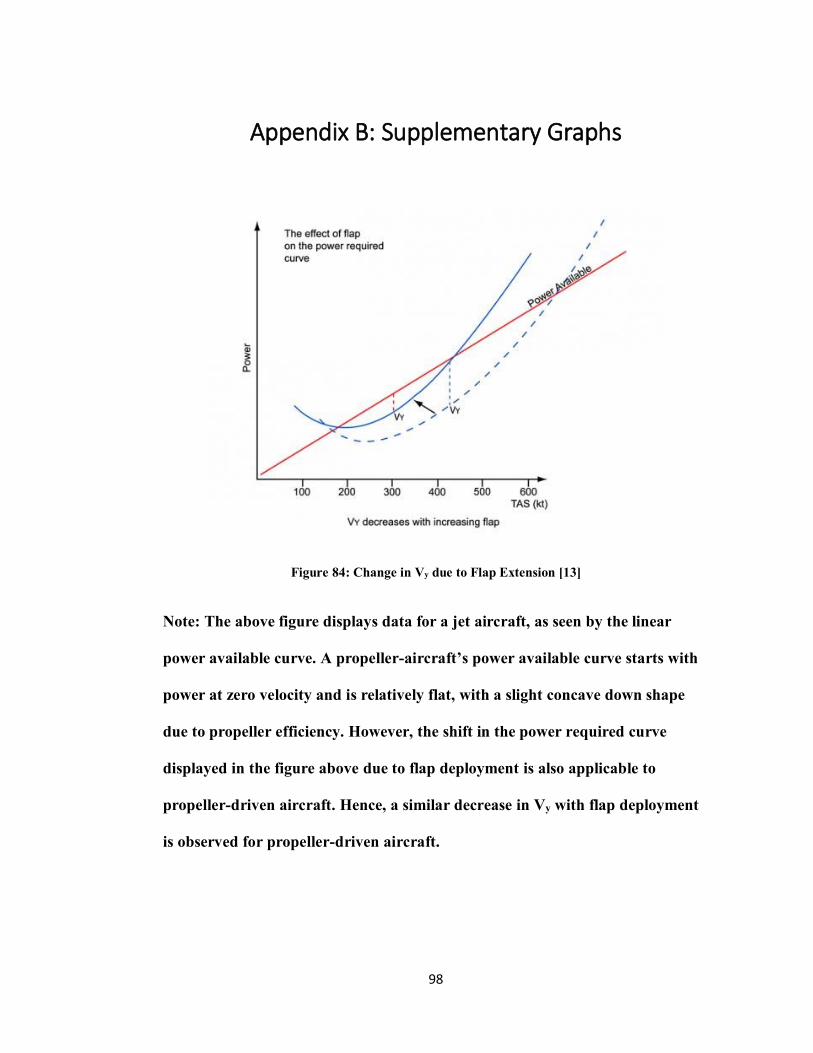
98

Appendix B: Supplementary Graphs

Figure 84: Change in Vy due to Flap Extension [13]

Note: The above figure displays data for a jet aircraft, as seen by the linear

power available curve. A propeller-aircraft’s power available curve starts with

power at zero velocity and is relatively flat, with a slight concave down shape

due to propeller efficiency. However, the shift in the power required curve

displayed in the figure above due to flap deployment is also applicable to

propeller-driven aircraft. Hence, a similar decrease in Vy with flap deployment

is observed for propeller-driven aircraft.

99

Figure 85: Altitude Effect on Vy [14]

Investigating the Effects of Altitude and Flap Setting on ...

Documents

Transcript of Investigating the Effects of Altitude and Flap Setting on ...