Investigating parental monitoring, school and

family influences on adolescent alcohol use

End of project report for Alcohol Research UK

March 2013

Dr. Kathryn Higgins

Dr. Mark McCann

Dr. Aisling McLaughlin

Ms Claire McCartan

Dr. Oliver Perra

Institute of Child Care Research

Queen’s University Belfast

Introduction

Adolescence is a dynamic developmental period, during which young people develop

behaviours and habits that affect their health and social outcomes. Teenage drinking in

particular has become a major public health concern, with under-18s consuming more

alcohol than in previous generations, seduced by a new range of alcoholic drinks designed

for the brand-savvy youth consumer. A recent UK survey indicated that 70 per cent of 13-14

year olds and 89 per cent of 15-16 year olds had, had an alcoholic drink; the most common

age for a first drink was 12 to 13 years old, usually when with an adult and celebrating a

special occasion (Bremner et al., 2011). Adolescent alcohol use has been associated with

delinquency and violence (Peleg-Oren et al., 2009; Felson, Teasdale & Burchfield, 2008;

Ellickson, Tucker & Klein, 2003); early sexual debut and risky sexual behaviour (Fergusson &

Lynskey, 1996; Cavazos-Rehg et al., 2010) and poor academic performance (Balsa, Giuliano,

& French, 2011; Peleg-Oren et al., 2009; Barry, Chaney & Chaney, 2011).

Within the social context navigated by these adolescents attempts to identify the

behavioural determinants of teenage alcohol use, has stimulated much interest. A thorough

understanding of adolescent substance use must consider the complex interplay among

adolescents, their families, and their social environments (Cleveland, Feinberg & Greenberg,

2010). The family is a key influence on children’s and young people’s behaviour (Sondhi &

Turner, 2011); however, interventions at the level of the family that aim to reduce adolescent

behaviour have weak effects overall (Smit et al., 2008). As young people get older, primary

influences tend to move from the parents to the peer group and other societal factors

(Armsden, and Greenberg, 1987). Several seminal studies have demonstrated that

disengagement from pro-social entities (such as school) and either simultaneous or

subsequent engagement with anti-social entities (e.g. delinquent or substance-using friends)

are critical contributors to adolescent alcohol use (Henry, Oetting, & Slater, 2009). None the

less, parental and family factors still hold huge sway over how much influence these other

factors have, and at which stages they will start to predominate (Velleman, 2009).

Understanding how these interactions play out between family, peer and school processes,

requires further investigation.

Parental monitoring

For parents of teenagers, negotiating adolescence is a notoriously difficult task requiring the

development of parenting practices such as ‘parental monitoring.’ Parental monitoring refers

to a parents’ knowledge of their child’s whereabouts, activities and associations or social

connections (see Patock-Peckham et al., 2011, Ledoux et al., 2002; Stattin & Kerr, 2000;

Soenens et al., 2006; Borawski et al., 2003). Evidence drawn from an extensive body of

literature connects low levels of parental monitoring to a wide range of antisocial and risk

behaviours (e.g. Ary et al., 1999). Of particular relevance to this study, low parental

monitoring has been associated with: teenage alcohol use (Fosco et al., 2012; Pokhrel et al.,

2008; Velleman, 2009; Bahr, Hoffman & Yang, 2005, Bremner et al., 2011; Barnes & Farrell,

1992; Nash, McQueen & Bray, 2005; De Haan & Boljevac, 2009); initial levels of alcohol

misuse and rates of increase in alcohol misuse (Barnes et al., 2000; Barnes et al., 2006; Ryan,

Jorm & Lubman, 2010); lifetime alcohol use (Habib et al., 2010); frequent drinking (Bremner

et al., 2011; Marsden et al., 2005); excessive, risky, binge or problematic drinking (Bremner et

al., 2011; Piko & Kovács, 2010; Habib et al., 2010; Arata, Stafford & Tims, 2003; Gossrau-

Breen, Kuntsche & Gmel, 2010).

Few studies have identified attempted to identify patterns of parental monitoring. Tobler &

Komro (2010) identified four trajectories of monitoring (and communication) (in a sample of

2621, 6th-8th graders): high (76.4%), medium (9.1%), decreasing (6%) and inconsistent (8.5%).

Relative to those with high monitoring/communication, youth in the decreasing and

inconsistent trajectories were at significantly greater risk for past year and past month

alcohol use. Cleveland et al. (2005) reported effective parenting (including monitoring the

child’s activities) protected adolescents from subsequent alcohol use more than five years

later, and, these protective effects were strongest among families residing in high-risk

neighbourhoods. The effects of parental monitoring may also confer differential risks for

sons and daughters. Griffin et al. (2000) found an association between increased parental

monitoring and less drinking among boys in a sample of 228 sixth-grade students. Borawski

et al. (2003) also reported an association between high parental monitoring and less alcohol

use among males; parental monitoring had no effect on female behaviour (692 adolescents

in 9th & 10th grades); others (see Ledoux et al., 2002; Fosco et al., 2012) have reported no

gender differences. The degree of influence of parental monitoring (or knowledge), in the

context of other family variables, has been demonstrated across studies. Griffin et al. (2000)

indicated parental monitoring as having the strongest protective effect of any parenting

variable in a study which also investigated parent-child communication and parental

involvement. Ledoux et al. (2002) reported other family variables such as the family structure,

maternal and parental relationships, showed greatly reduced significance, once parental

knowledge was taken into account.

The direction of the association between parental monitoring and child alcohol use is not

always specified or investigated in the extant literature, primarily due to the use of cross-

sectional data. As the data for this study was collected over time, we can investigate the

temporal ordering of the association between these factors, and thus try and unpick the

causal relationships, or the extent to which one factor influences the other. In addition to the

idea that low parental monitoring leads to higher adolescent alcohol use, it may be

hypothesised that adolescents who use alcohol heavily may elicit increased levels of

monitoring from their parents (i.e. reverse causation). Once adolescents begin ‘normative’

drinking in social settings without their parents, they may modify their behaviour around

their parents asserting greater autonomy and encouraging their parents to permit greater

independence in order to facilitate peer socialisation. Despite an explicit call from the

creators of the standard parental monitoring scales to assess these youth-driven processes,

few studies have used longitudinal data to do so (Kerr, Stattin & Burk, 2010) The Belfast

Youth Development Study, having collected data on parental monitoring and alcohol use

across the early adolescent years is eminently suited to clarifying the direction of association

and clarify the extent to which these causal or reverse causal mechanisms hold true.

Child disclosure

Adolescence typically portents a shift away from parental reliance to greater autonomy, or a

move from asymmetric to more symmetric relationships in which parents relax control (e.g.

Keijsers et al., 2009) and adolescents gradually disclose less information in order to reduce

parents’ authority and gain more autonomy (Finkenauer, Engels, & Meeus, 2002). Although,

initially operationalised as the ‘tracking and surveillance of children’s behaviour,’ Stattin &

Kerr’s (2000) definition of parental monitoring was extended to assess not only the parent’s

knowledge but also the source of their knowledge (see Kerr & Stattin, 2000). This

reinterpretation of ‘parental monitoring’ stems from their study of approximately seven

hundred, 14 year olds which reported parental knowledge came mainly from child disclosure

about their unsupervised activities outside the home whereby child disclosure was the

source of knowledge that was most closely linked to broad and narrow measures of

delinquency. More recently, Kerr, Stattin, & Burk (2010) revisited this hypothesis using

longitudinal data, which also indicating youth disclosure was a significant predictor of

parental knowledge and neither measure of parents monitoring efforts-control or

solicitation were significant predictors. Soenens et al. (2006) argue, although studies such as

those by Kerr and colleagues, indicate parental knowledge has more do to with adolescents’

self-disclosure than with parents active monitoring, this may be due to self-disclosure being

influenced by parents’ rearing style. In their investigation, characteristics such as high

responsiveness, high behavioural control and low psychological control were associated with

self-disclosure among students (Soenens et al., 2006). In addition, SEM analyses revealed

parenting is both indirectly (through self-disclosure) and directly associated with perceived

parental knowledge but not directly related to problem behaviour (including alcohol use) or

affiliation with peers engaging in problem behaviour. Gender differences are also apparent.

A study by Waizenhofer, Buchanan & Jackson-Newsom (2004), indicated mothers knew

more about adolescents’ activities than did fathers and were more likely than fathers to gain

information by active supervision or voluntary disclosure from the adolescent. Fathers were

more likely than mothers to receive information via their spouses/partners. Overall, these

studies suggest that adolescents contribute actively to parental monitoring by managing

strategically the information they disclose.

Parental solicitation

Studies on parental monitoring suggest parents solicit more information from girls than

boys (according to the children, not the parents) (Stattin & Kerr, 2000). While a number of

studies have investigated the role of solicitation in teenage alcohol use (e.g. Jimenez-Iglesias

et al., 2013), to our knowledge, no evidence of an association between parental solicitation

and teenage drinking has been reported. Results from a longitudinal study of adolescent

alcohol use and parental source of knowledge, indicated parents active efforts to (control

their youths or to) gain information through solicitation do not appear to have an effect in

reducing their children’s drinking behaviour (Stavrinides, Georgiou & Demetriou, 2010). The

extant literature indicates children will reduce maladaptive behaviours when they are free to

share their thoughts with their parents in a free and uncontrolling manner (Stattin & Kerr,

2000).

Parental control

The theoretical perspective of social control theory (Gottfredson & Hirschi, 1990) argues that

a lack of parental monitoring and control plays a pivotal role in determining adolescents’

involvement in deviant behaviour and substance use due to weakened ties with family,

school and other aspects of society that serve to diminish one’s propensity for deviant

behaviour. . According to this perspective, parental monitoring efforts can be effective in

reducing opportunities for young people’s association with deviant peers and risk taking

(e.g. Dishion & McMahon, 1998). Lax parental control has been associated with increased

drinking (Foxcroft & Lowe, 1991) and problematic alcohol use (McKay et al., 2010) among

adolescents. van der Vorst et al., (2006), reported strict parental control was related to lower

engagement in alcohol use among adolescents. Others have reported evidence of a possible

curvilinear relationship between control and adolescent drinking. Stice, Barrera & Chassin

(1993), found a negative linear relationship between parental control, parental support and

adolescent alcohol use and both control and support were prospectively related to

adolescent alcohol use. The authors concluded adolescents who receive either extreme of

parental support or control are at risk for problem behaviours.

Parental attachment

One factor that would seem likely to influence the relationship between monitoring and

alcohol use is parental attachment (Barnes et al., 2000). Problematic parent-child interactions

may disrupt parents’ attempts to monitor and control their children, and they may also be

less open and honest in their activities. This disruption in attachment itself may lead to

harmful alcohol use, above and beyond the risk conferred by different patterns of

monitoring attributable to poor attachment. Family bonding or attachment appears to

protect against alcohol use (Velleman, 2009; Anderson & Henry, 1994; Sokol-Katz, Dunham

& Zimmerman, 1997). van der Vorst et al. (2006) found an association (cross-sectional)

between parental attachment and early development of adolescent alcohol use (11-14 year

olds). The study used 3 waves of data (baseline, 6 months, 12 months) and longitudinal

analyses using SEM suggested a good attachment relationship between parent and child

does not prevent adolescents from drinking. In terms of moderating effects, parental

attachment did not moderate the association between parental control and an early

development of alcohol use.

In this study, we have information on overall levels of parental monitoring of child activity,

and information on the three methods of gaining monitoring information mentioned above.

We propose to explore how each of these methods of monitoring

Peer influences

The influence of peer or peer alcohol use on teenage drinking has been widely reported

(Dickens et al., 2012; Capaldi et al., 2009; Shortt et al., 2007; Simons-Morton, 2004, Dishion &

Owen, 2002; Borsari & Carey, 2001; Barnes et al., 2006; Donovan et al., 2004; Trucco, Colder

& Wieczork, 2011, Stoolmiller et al., 2012; Windle, 2000; Rai et al., 2003; Rawana & Ames,

2012; Andrews et al., 2002; Henry, Oetting & Slater, 2009). Evidence suggests young people

are more likely to drink, drink frequently and drink to excess if they spend more than two

evenings a week with friends (Bremner et al., 2011) or have friends who drink (Goodman et

al., 2011; Bremner et al., 2011). Once again, gender differences are apparent. Friends’

drinking has been more strongly related to alcohol use in girls, compared to boys, and in

adolescents with opposite-sex friends, compared to adolescents with only same-sex friends

(Dick et al., 2007). Peer relationships have been reported to have greater effects on drinking

behaviour in female than in male adolescents (Yeh, Chiang & Huang, 2006; Simons-Morton

et al., 2001). Gaughan (2006), investigating best friend dyads, reported adolescents in same-

sex best friendships influenced one another mutually, boys in mixed-sex best friendships had

an influence over their female friends’ drinking patterns while girls did not have any effect

on their male friends drinking behaviour. Others suggest having norm breaking friends is

predictive of alcohol use among girls and young boys (Branstrom, Sjostrom & Andreasson,

2007). Perceived peer group drinking has also been demonstrated as a significant individual

level predictor of drinking initiation (Stock et al., 2011) and increases in use (Capaldi et al.,

2009).

In keeping with the general literature on development, adolescents appear to become

increasingly socialised by their peers, often at the expense of parents’ efforts (Latendresse et

al., 2008). However, Velleman (2009) argues the family can continue to be a moderating

influence throughout adolescence and even young adulthood. A number of studies have

examined interactions between family and peer influences demonstrating these moderating

effects (e.g. Nash, McQueen & Bray, 2005). Families which are characterised by low levels of

parental monitoring and exposure to substance using peers may serve as a marker of

increased vulnerability (Velleman, Templeton & Copello, 2005; Duncan et al., 1998; Dishion

& Owen, 2002; Kuntsche & Jordan, 2006) playing a pivotal role in the onset and

development of young people’s alcohol use. Furthermore, parental monitoring is reportedly

a protective factor for the selection of substance using friends (Cohen, Richardson & LaBree,

1994). Nash, McQueen & Bray (2005) demonstrated peer influence (use of alcohol by same

age peers and friends, friends’ approval of drinking) had a stronger effect on subsequent

adolescent behaviour than family environment. Family environment however influenced

adolescents’ peer characteristics: positive family environment was related to fewer peers that

drank alcohol and less perceived peers’ approval of drinking. Wood et al. (2004) reported

significant associations between both peer and parental influences and alcohol involvement

and showed that parental influences moderated peer influence drinking behaviour such that

higher levels of perceived parental involvement were associated with weaker relations

between peer influences and alcohol use and problems. Simons-Morton & Chen (2005)

reported that although the growth in the number of friends who drink was positively

associated with adolescent drinking, parental (involvement and) monitoring (and

expectations) over time provided direct protective effects against drinking progression and

indirect effects by limiting increases in the number of friends who drink. Bergh, Hagquist &

Starrin (2011) found high levels of peer activity were associated with higher frequencies of

alcohol use; although the effects of relations with parents were modified by peer activity

frequencies, high levels of parental monitoring were significantly associated with lower

frequencies of alcohol use, regardless of peer activity frequencies. Trucco, Colder &

Wieczorek (2011) in a study of 11-13 year olds, reported high levels of peer delinquency

prospectively predicted perceived peer approval and use of alcohol and that peer approval

and use of alcohol prospectively predicted initiation of alcohol use. However, there was no

support for parental (warmth or) control as moderators of peer influence. Kim & Neff (2010)

reported both direct and indirect effects of parental monitoring on adolescent alcohol use;

peer influence mediated the relationship between parental monitoring and adolescent

alcohol use. Schinke, Fang & Cole (2008) found associations between girls’ use of alcohol,

who their friends were and their mothers knowledge of their whereabouts and companions.

Studies such as Latendresse et al. (2008) have demonstrated that the mediating role of

parenting decreases between early and later adolescence.

Attachments or emotional closeness to parents may also be mediated peers. Kelly et al.

(2011) found that for girls, the effect of emotional closeness to mothers on alcohol use was

mediated by exposure to high-risk peer networks. Overall, peer drinking networks showed

stronger direct risk effects than family variables (i.e. emotional closeness, family conflict,

parent disapproval of alcohol use). Martino, Ellickson & McCaffrey (2009) reported across a

variety of peer contexts (including stable high association with drinking peers, stable low

association and increasing association), youth were at lowest risk for developing problematic

patterns of heavy drinking when they perceived that their parents maintained strong

disapproval of substance use throughout adolescence.

Few studies have investigated whether the parenting experienced by one’s friends also

affects one’s own use. Cleveland et al. (2012) identified 897 friendship groups among 7,439

ninth grade students. Adolescent substance use in 10th grade was significantly related to

parenting behaviours of friends’ parents, after controlling for adolescents’ reports of their

own substance use and their own parents’ behaviours at the 9th grade level. These

associations were particularly strong for parents’ knowledge about their children and use of

inconsistent discipline strategies. Some, but not all, of the main effects of friends’ parents’

parenting became non-significant after friends’ substance use in ninth grade was included in

the model. Nonetheless, the findings suggest that the parenting style in adolescents’ friends’

homes plays an important role in determining adolescent substance use.

School Influences

The school is the primary institution outside the family within which the development of

adolescents can be directed and shaped (Simons-Morton et al., 1999). Gottfredson and

Hussong (2011) examined changes in drinking patterns among adolescents as they made the

(stressful) transition to high school. Those adolescents who reported less parental

involvement were at a higher risk of drinking, highlighting the transition as an important

intervention leverage point for those who lack adequate parental support to help them cope

with day to day changes. Cleveland, Feinberg & Greenberg (2010) indicated the benefit of

belonging to a well-functioning family is more influential for students attending schools

characterised by higher-than-average aggregated levels of protection compared to students

attending schools of lower-than-average protection. Overall, family-level factors offered less

protection for students in relatively high-risk school contexts.

Fletcher (2012) investigated peer influences on adolescent alcohol consumption among

students in different grades within the same school-results indicated that a 10 per cent

increase in the proportion of classmates who drink increases the likelihood an individual

drinks by five percentage points. This paper also provided evidence of peer effects in

problem drinking such as binge drinking and drunkenness. Clark & Loheac (2007) examined

risky behaviour among American adolescents (collected as part of the Add Health survey,

1994-1996) and reported that even controlling for school fixed effects, risky behaviours were

correlated with lagged peer group behaviour. These peer group effects were strongest for

alcohol use with young males being more influential than young females. The study

suggested both boys and girls follow boys, as the probability of having had an alcoholic

drink in the previous 12 months was, within the school, positively correlated with the

percentage of boys in the same school year who drank one year ago. Mrug et al. (2010)

investigated the effect of school-level substance use on early adolescent alcohol, tobacco

and marijuana use among 452 students attending 49 public middle schools in a single

metropolitan area. Only school-level rates of cigarette smoking were associated with

individual smoking. However, this study focused on early adolescence and other studies (e.g.

Rehm et al., 2005) have found associations between school-level use of alcohol and

individual students’ use in high school (across adolescence). Rehm et al. (2005) reported

both the average and volume of alcohol consumption and patterns of drinking influenced

alcohol-related problems at the student level. Lundborg (2006) investigated school-class

based peer effects in binge drinking (smoking and illicit drug use) among 12-18 year old

students. Positive peer effects were found, and by introducing school/grade fixed effects, the

estimated peer effects were identified by variation in peer behaviour across school-classes

within schools and grades, implying that estimates were not biased due to endogenous

sorting of students across schools.

Internationally, studies have indicated urban-rural divides in alcohol consumption among

adolescents. Donath et al. (2011) reported higher life-time and 12 month (previous year)

prevalence rates of alcohol use among adolescents in rural areas in Germany; the authors

suggested fewer opportunities for engaging in interesting leisure activities than adolescents

in cities, as a reason for higher alcohol use rates. Adolescents living and attending school in

deprived areas are at increased risk of associating with deviant adolescents (adolescents

from malfunctioning families) and, through association with these adolescents, are at

increased risk of deviant behaviour such as heavy drinking themselves, regardless of their

own family relationships (Bernburg, Thorlindsson, & Sigfusdottir, 2009). Stock et al. (2011)

investigated the relationship between school district-level factors and the initiation of

alcohol drinking among Danish youth. Adolescents were more likely to initiate alcohol

consumption in school districts with higher farming land use and less likely in those with

higher proportions of private apartment buildings. Other school district factors were not

associated with drinking initiation when they controlled for individual level factors. De Haan

& Boljevac (2009) investigated community attitudes and behaviours in the context of

adolescent drinking in rural environments. Results indicated adolescent drinkers had higher

perceptions (compared to non-drinkers) of peer, parental and overall community drinking as

well as lower levels of parental closeness. Adolescent perceptions of peer use were more

accurate than either parents or school officials. Parents were significantly less likely to

perceive adolescent alcohol use as a problem than other community adults; school officials

were most likely to perceive it as a problem. Overall, school officials’ perceptions of

adolescent alcohol use were more related to actual adolescent use than were parental

perceptions of adolescent use.

Project Aims

This study aims to:

test different causal hypotheses explaining the longitudinal relationship between

parental monitoring and alcohol use trajectories

test the role of peer- and school-level factors in influencing individual drinking

trajectories and monitoring

investigate how patterns of monitoring dimensions (e.g. parental control and

child disclosure) and their association with alcohol use change when considering

other factors

To achieve these aims, this study was divided into a number of sections; path analysis

investigating how parental monitoring and alcohol use are related; multilevel modelling,

investigating how alcohol use, and parental monitoring varies between different schools,

and finally; structural equation models to assess the direct and indirect associations between

monitoring and other important family characteristics.

Methods

This study used data from the Belfast Youth Development Study, a longitudinal study of

substance use during adolescence. Between 2000 and 2011, children attending over 40

schools, colleges and special educational programmes were given questionnaires on a range

of personal, social, health and substance use issues. Seven data sweeps took place during

this period. Pupils were in their first year of secondary school (around age 11) at the start of

the study (academic year 2000/2001), were surveyed annually until 2006/2007 (around age

17) whether they were still attending school, were in a further education college, or no

longer in education. They were surveyed again around ten years since they first participated

(2011). This report is based on data from the first five years of the study. Where possible,

information was linked longitudinally for pupils. The response rate across the sweeps of the

study was complex. In year two, several new schools joined that had not been surveyed in

year one. Teachers at some schools were participating in industrial action during year four

and hence pupils at these schools were not surveyed.

Figure 1: Response rates for the first five years of data collection

Figure 1 shows the total numbers contacted at each sweep, how many provided data in all

years, and how many new entrants, leavers, and rejoiners there were in each year. The right

hand side also shows the cumulative number of participants. Across the five years of the

study, a total of 5,371 people participated.

Study Variables

This study draws on data from years one to five of the study. Demographic, health,

socioeconomic, and family characteristics measures were taken from each year where

responses were available. The mental health measure used was the strengths and difficulties

questionnaire (SDQ). The SDQ is a mental health screener for children and adolescents. The

SDQ was asked in years one and four of the study.

The inventory of peer and parental attachment was also included in analysis, this scale

includes questions such as “my parents respect my feelings” and “I trust my parents”. This

12 item scale was asked on a three point scale in the first year of the study, and a five point

scale in later years of the study. Analysis used standardised scores, with a mean of zero and

sd of one.

Respondents were asked questions about the number of cars at their household (None, one,

two or more), number of family holidays (none, one, two, three or more), parental

employment status (None, part-time, full-time for mother and father), whether they had a

bedroom to themselves (yes/no), the type of house they lived in (apartment, terraced, semi

detached, detached), and eligibility for free school meals (signifying parental receipt of

benefits; yes/no). Principal components analyses were used to create affluence measures (1)

based on these items for each year. Number of family holidays was dropped, as it loaded

onto a separate factor, decision to take holidays appears to be largely independent of

socioeconomic position. A single component modelled around 35% of the variance in the

affluence indicators (Rho; year 1 0.38; year 2 0.39; year 3 0.35; year 4 0.34; year 5 0.37). In all

years, the first component had an eigenvalue between 2.03 (year 4) and 2.31 (year 2).

Eigenvalues for all other components fell below one. Analyses used affluence scores

computed within each year.

Respondents were asked with whom they lived in each year of the study. Responses were

grouped into lives with; both biological parents; a reconstituted family (one biological & one

step/foster parent); Single parent; and complex/other (predominantly siblings or

grandparents) . Living arrangements in year five of the study were used in analysis. We did

not study change in living arrangements specifically, although any parental separation prior

to year five will be represented by living arrangements in year five, although not when this

occurs. Where living arrangement information was not available in year five, the previous

year’s information was used in its place. As this study focussed on the importance of family

relationships, people living in complex/other household types were not included in analysis.

Analytical variables

The two main variables of interest in this study are parental monitoring and alcohol use.

Each year, participants were asked about how frequently they drank alcohol. Responses for

each year were coded; does not drink; rarely drinks, drinks monthly, drinks weekly or more

frequently, and missing/no info. Stattin & Kerr’s (2000) measures of parental monitoring

were asked in each year. Four sets of questions were asked; overall parental monitoring, and

three methods of monitoring children’s behaviour, child disclosure of information, parental

solicitation of information, and parental control of child activity. The monitoring component

included questions such as ‘do your parents know what you do with your free time’ and ‘do

your parents know who you have as friends during your free time?’. The child disclosure

component centred on information offered to parents without being asked; ‘Do you talk at

home about how you are doing in different subjects at school’, and ‘do you keep a lot of

secrets from your parents about what you do in your free time?’. The parental solicitation

component, designed to find out how much parents ask their children about what they do

included ‘how often do your parents talk with the parents of your friends’, and ‘how often do

your parents start a conversation about things that happened during a normal day at

school?’. The parental control component included ‘do you need to have your parents’

permission to stay out late on a weekday evening’, and ‘if you have been out late one night

do your parents require you to explain what you did and who you were with?’.

Phase 1: Parental Monitoring and Alcohol Use: Causation and path analysis

In order to investigate the causal processes underlying the association between parent-child

interaction and child alcohol use, we fitted a series of path analytic models. Path models are

a form of Structural Equation Model. In this case, the models assessed the association

between parental monitoring and subsequent alcohol use, while also assessing alcohol use

and subsequent parental monitoring.

The models were built up as follows: Focussing on year one monitoring, we estimated its

association with alcohol use in years two, three, four, and five (i.e. each subsequent year)

using a series of ordinal logistic regression models. Year two monitoring was associated with

each subsequent year (years three, four and five) and the same format for year three and

four. These regression models were also adjusted for prior alcohol use (i.e. Year five on year

four alcohol use, year four on year three etc). The exact same format of time-lagged

regression models were used to estimate how alcohol use in each year was associated with

subsequent monitoring, after accounting for prior levels of monitoring. These models were

then re-estimated after controlling for gender, mental health, affluence, parental attachment

and living arrangements. On the basis of these fully adjusted models, the final models

presented in the results section below were obtained by estimating only those paths which

were significant at p<0.1 if a control variable or P<0.05 if an analytic variable. Interaction

terms between gender and analytic variables were used to assess if the effect of monitoring

on alcohol use (or vice versa) varied comparing males and females.

This format of modelling was performed looking at the overall monitoring scale, and for

each of the three monitoring method scales (solicitation, control, child disclosure). All

models were adjusted to account for clustering at the school level.

Phase 2: Parent, Peer and School influences

The next set of models built upon the final models derived from the first stage of analysis.

These models investigated between-school variation in alcohol use (and its association with

monitoring), and also between-school variation in monitoring (and its association with

alcohol use). Given that there is a trend for increasing alcohol use at older ages, variation

between schools was assessed in the last year of the study, when presumably most

respondents will have begun drinking, thus maximising the difference between the lightest

and heaviest drinking individuals, and thus, by extension making it easier to assess

differences between lighter and heavier drinking schools. These models included all

variables that were identified as associated with alcohol use / monitoring in the first set of

models. In addition, the following characteristics of the schools were included; school gender

(boys only, girls only, co-educational); catholic vs. state maintained; geographical location

(Belfast, Ballymena, Downpatrick); overall level of alcohol use in the school (proportion of

weekly drinkers); overall level of parental monitoring in the school (mean monitoring score

within school).

Phase 3 – Aspects of Monitoring

Latent profile analyses were used to identify if there were distinct profiles of responses to

the four parental monitoring scales, example profiles could be ‘very low on all scales’; ‘very

high on all scales’; ‘high disclosure but low control’ and so on. The analyses assessed the

response pattern for all respondents, and determined how many patterns of responses, or

‘profiles’, would best account for the variation between respondents. Models were

constructed ranging from two profiles through to ten profiles. These models were compared

using the Sample Size Adjusted Bayes Information Criterion (SSBIC) and Entropy fit indices,

and the Vuong-Lo-Mendell-Rubin test for comparing models. The SSBIC measure gives a

measure of relative fit of the observed responses to those predicted by the models being

compared (i.e. how accurately does a two profile model describe the actual range of

individual responses, by comparison to a three profile model). The entropy measure

indicates how successful the model is in determining which profile a respondent belongs to.

Where a model can determine with accuracy which profile all respondents belong to, the

value of entropy is close to 1, and this gives an indication that the a model explains the

response patterns for individuals well. Where a model performs very poorly in predicting

profile membership, the value of entropy is close to zero and this gives us less confidence

that the profiles determined by the model are a strong representation of how individuals

responded. Entropy values greater than 0.8 are usually considered a sign that the classes

specified by the model represent individual’s responses well; in other words, lending

confidence to the idea that in the general population, people follow certain patterns of

behaviour in relation to monitoring levels. Mplus 6 was used for these analyses.

The final stage of analysis looked at the inter-relationship between different elements of the

parent child relationship and alcohol use; in particular the relationship between monitoring

and parental attachment. Structural equation models were used to assess firstly the

relationship between attachment and alcohol use, and also monitoring and alcohol use,

secondly, these models assessed the association between attachment and parental

monitoring, and thirdly, they assessed the indirect effect of parental attachment on alcohol

use, due to its influence on monitoring. The outcome measure for these models was a

continuous latent variable indicating propensity to drink frequently, with lower scores

indicating very low rates of drinking, and higher scores indicating more frequent drinking.

This measure was based on the frequency of drinking measure as used for other models, and

the frequency of being drunk. This measure was used in place of either single frequency

measure to deal with computational limitations. While Mplus could perform the path

analyses detailed above a drinking frequency measure based on categories, the assessment

of indirect associations between variables requires continuously distributed outcome

measures. The latent variable based on these two measures was left skewed; most

respondents scored quite highly (i.e. drinking somewhat regularly) with less respondents

with very low( drinking very infrequently) or very high scores (getting drunk very frequently).

The left skew demonstrated that it was much more common to drink less than it was to get

drunk very frequently. Residual diagnostics for regression of this measure of predictors

showed that the residuals followed a normal distribution; as such, this variable adhered to

the assumptions underpinning the Structural Equation Model approach and provided an

appropriate alternative outcome measure to the four category drinking frequency outcome.

These models assessed the associations between year four monitoring score, year four

attachment score, and alcohol use based year five frequency of drinking and frequency of

drunkenness. The models then accounted for prior drinking (using year four drinking and

drunkenness frequency measures), and then further accounted for the confounding variables

as specified above.

Results

Table 1 shows the distribution of individual attributes and family characteristics that were

used in analysis. In total, there were 4,775 included in analysis.

There was a reasonably even split between boys (2,257) and girls (2,518) in the sample.

Around 6% of the cohort showed some signs of mental health problems, this proportion was

similar at both time points when it was asked (approx. age 11 and 14). Almost three quarters

of the cohort lived with both biological parents, 19% lived with one parent only, and around

9% lived with a parent plus step-parent, parent’s partner, foster parents etc. The living

arrangement variable was based on living arrangements at the end of the study period

(around age 16), as such it would capture change in family structure before this time point.

We did not analyse when family structure changed. Where no information was available

from the year five survey, the previous year’s data was used instead. As the focus of the

study was on the effect of parental monitoring, 464 individuals were excluded as they did

not live with parents. As analysis also looked at between-school variation, a further 132

respondents that did not attend mainstream schools were also removed from analysis. All

remaining individuals were analysed, even where they did not provide responses in all waves

of the study.

Parental attachment was assessed on a different scale in year one compared to years three

and four. For this reason, scales were standardised to have a mean of zero and standard

deviation of one within each year, so that the statistical measures for the effect of

attachment would be comparable across years.

Table 1: Individual and family characteristics for 4,775 respondents

Variable Frequency

(% of total)

Gender

Male 2,257 (47.3)

Female 2,518 (52.7)

Mental Health

Year 1 – SDQ

Normal 3,116 (65.3)

Abnormal 310 (6.5)

Missing 1,349 (28.3)

Year 4 – SDQ

Normal 3,485 (72.9)

Abnormal 309 (6.5)

Missing 981 (20.5)

Living Arrangements

Biological parents 3,442 (72.1)

Reconstituted family 428 (9.0)

Single parent 905 (19.0)

Parental Attachment Mean (s.d.) Number of responses

Year 1 16.9 (3.99) 3,391

Year 3 61.9 (20.6) 4,267

Year 4 62.7 (21.5) 3,752

Affluence

Year 1 3.6 (1.39) 3,349

Year 2 3.5 (1.44) 3,841

Year 3 3.5 (1.43) 4,088

Year 4 3.4 (1.45) 3,763

Year 5 3.4 (1.45) 3,634

Total 4,775

Table 2 shows the rates of alcohol use across the five years of the study. In the early years of

the study, very few respondents drank frequently, although a large proportion reported

having tried alcohol. In later years, a greater proportion of the cohort reported drinking

alcohol every week or more often; from years one to five, the respective proportions drinking

weekly were 4%, 11%, 21%, 27% and 34%.

Table 2: Frequency of alcohol use across five years for 4,775 respondents

Alcohol use Male Female Total

Year 1

None 493 (22) 547 (22) 1,040 (22) Rarely 1,103 (49) 874 (35) 1,977 (41)

Monthly 92 (4) 63 (3) 155 (3) Weekly or more 135 (6) 45 (2) 180 (4)

Missing 434 (19) 989 (39) 1,423 (30)

Year 2 None 607 (27) 764 (30) 1,371 (29)

Rarely 749 (33) 809 (32) 1,558 (33) Monthly 224 (10) 265 (11) 489 (10)

Weekly or more 270 (12) 267 (11) 537 (11) Missing 407 (18) 413 (16) 820 (17)

Year 3

None 505 (22) 513 (20) 1,018 (21) Rarely 707 (31) 863 (34) 1,570 (33)

Monthly 352 (16) 392 (16) 744 (16) Weekly or more 471 (21) 521 (21) 992 (21)

Missing 222 (10) 229 (9) 451 (9)

Year 4 None 155 (8) 147 (6) 322 (7)

Rarely 545 (24) 606 (24) 1,151 (24) Monthly 362 (16) 404 (16) 766 (16)

Weekly or more 552 (24) 745 (30) 1,297 (27) Missing 623 (28) 616 (24) 1,239 (26)

Year 5

None 121 (5) 120 (5) 241 (5) Rarely 370 (16) 415 (16) 785 (16)

Monthly 365 (16) 419 (16) 784 (16) Weekly or more 736 (33) 875 (35) 1,611 (34)

Missing 665 (29) 689 (27) 1,354 (28)

Total 2,257 2,518 4,775

Table 3: Correlation coefficients for Parental Monitoring scale across five years Year 1 Year 2 Year 3 Year 4 Year 5

Year 1 ~~~ Year 2 0.29 ~~~ Year 3 0.15 0.26 ~~~ Year 4 0.00 0.10 0.04 ~~~ Year 5 0.02 0.09 0.04 0.25 ~~~

Table 4: Correlation coefficients for Parental Control across five years Year 1 Year 2 Year 3 Year 4 Year 5

Year 1 ~~~ Year 2 0.29 ~~~ Year 3 0.15 0.25 ~~~ Year 4 0.00 0.10 0.04 ~~~ Year 5 0.02 0.10 0.04 0.26 ~~~

Table 5: Correlation coefficients for Parental Solicitation across five years Year 1 Year 2 Year 3 Year 4 Year 5

Year 1 ~~~ Year 2 0.29 ~~~ Year 3 0.15 0.25 ~~~ Year 4 0.01 0.11 0.04 ~~~ Year 5 0.01 0.10 0.03 0.25 ~~~

Table 6: Correlation coefficients for Child disclosure across five years Year 1 Year 2 Year 3 Year 4 Year 5

Year 1 ~~~ Year 2 0.29 ~~~ Year 3 0.15 0.25 ~~~ Year 4 0.00 0.10 0.04 ~~~ Year 5 0.01 0.09 0.03 0.25 ~~~

Tables 3 to 6 show the correlation between monitoring scales over time. The difference in

correlation comparing year 1 and year 5 shows the extent to which monitoring levels change

with increasing age, it is these changes in monitoring levels, and the explanations for the

changes, that the path analyses presented below aim to explore

Monitoring, alcohol use, and paths of causation

Figure 2 below shows the results of fully adjusted models investigating the association

between overall levels of parental monitoring and alcohol use across the first five years. As

expected, the strongest associations in the model are the time-trend associations. Levels of

alcohol use in one year are highly predictive of use in the subsequent year. Similarly, prior

and subsequent levels of monitoring are closely associated. The overall reading of the model

suggests that there are bi-directional causal processes operating between alcohol and

monitoring, however these mechanisms are dependent on the age at which each occurs.

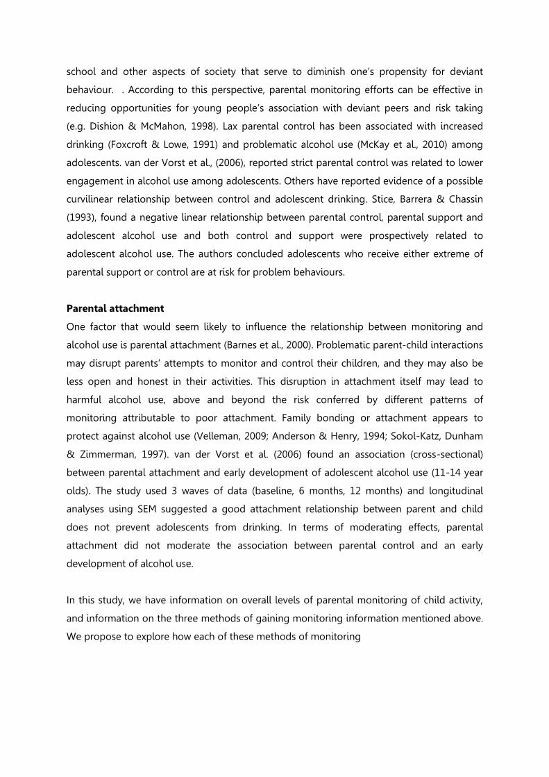
Figure 2: Path diagram showing associations between alcohol use and parental monitoring

Alcohol use Monitoring

Higher levels of alcohol use in any given year are associated with slightly lower rates of

parental monitoring in the subsequent survey year, suggesting that teenagers who drink

may change their relationship with their parents to exert greater autonomy, or provide their

parents with less information on their day to day lives. The magnitude of this effect is rather

small, with each step up in drinking rate (none to infrequently, infrequently to monthly,

monthly to weekly or more), monitoring decreased in the following year by around 0.05 of a

standard deviation in years 2,3 and 4. However, a step up in drinking in year 1 was

associated with a reduction in monitoring on 0.16 s.d. units, an effect three times larger than

that in any subsequent year.

Monitoring Alcohol use

Greater parental monitoring was associated with a lower rate of alcohol use in the

subsequent years. The magnitude and time-lag for the effects of monitoring on alcohol use

are of interest, in that they are somewhat at odds with the findings for the effect of alcohol

use on monitoring. A one unit increase in parental monitoring is associated with around a

20% lower rate of alcohol use in the subsequent year: this 20% reduction appears in all

years, with perhaps a slightly greater reduction at the youngest age, as appeared for the

alcohol use monitoring paths. The main difference is that high levels of parental

monitoring at a young age are directly associated with lower rates of drinking up to four

years later. That is, parental monitoring at a young age tends to encourage less frequent

drinking, even after taking into account natural changes in levels of autonomy and

monitoring, and the effect of monitoring at older ages.

Aspects of monitoring

The model in figure 2 demonstrated the inter-relationship between parental monitoring and

alcohol use, although more nuanced information on monitoring is available in the data. This

study used data from the parental monitoring scale (the overall level of knowledge of child

activities), and also three sources of monitoring information; parental solicitation, asking

information of their children; child disclosure, the young person volunteering information

about themselves; and parental control, the extent to which children must gain permission in

order to do something, thereby providing parents information on their activities and

whereabouts. Each of these dimensions is discussed below.

Parental solicitation

After accounting for confounding factors, parental solicitation showed very little evidence of

association with alcohol use. Higher levels of alcohol use in sweep one were associated with

lower parental solicitation in sweep two by around 0.1 sd units, while none of the other

causal paths showed any significant associations. Prior alcohol use was a strong predictor of

future alcohol use, as was the case in the model presented in Figure 2. Similarly, solicitation

was predictive of future levels of solicitation; in this case, the association between sweep

four and sweep five was greater than the association between sweep one and sweep two.

This suggests that there is greater change in levels of solicitation in early adolescence than

in later adolescence. Parents who talk frequently to their children about their activities by

sweep four continue to do so by sweep five (and low rates of solicitation similarly remain

low), whereas in early adolescence, prior levels of solicitation are less predictive of later

solicitation, as other factors have a greater impact, and greater levels of change in

solicitation occur.

Figure 3: Path diagram showing association between alcohol use and parental

solicitation

Parental control

Figure 4 shows the final model for alcohol use and its association with parental control. The

pattern of association for control is not dissimilar to that found with the general parental

monitoring scale, although it appears that alcohol use may have a greater influence on

controlling behaviours than was found for overall levels of monitoring. Higher levels of

alcohol use in sweep one, two and four were associated with between a 5% and 10% s.d. unit

reduction in levels of control by sweep five; similarly, alcohol reduced control behaviours in

the subsequent year, not just in sweep 5. This suggests that teenagers drinking more

influences the extent of later autonomy, and this effect may occur at any stage of adolescent

development, rather than being an effect of particularly early drinking, or an effect limited to

later ‘normative’ drinking, when it might be argued that parents would exert less control due

to their children’s age rather than their drinking habits. Higher parental control led to

around a 15% to 25% reduction in odds of drinking, the effect was most pronounced at

younger ages. The effect was reasonably long-lasting; higher parental control in year one

was associated with less frequent drinking up to three years later.

Figure 4: Path diagram showing association between parental control and alcohol use

Teenager disclosure

Higher levels of teenager disclosure were associated with lower alcohol use, although the

magnitude of association reduced with increasing age; the size of effect was around a 20% -

25% reduction on the subsequent year’s drinking for sweeps three and four, with little effect

on drinking by sweep five, and a larger effect (35% reduction) between the first and second

sweep of the study. High levels of disclosure at a younger age were also associated with

long-lasting reductions in alcohol use; as demonstrated by the coefficients linking sweep

one disclosure to sweep two, three and five rates of drinking.

Higher rates of alcohol use were associated with lower rates of disclosure in subsequent

years. Unlike for the disclosure Alcohol pathways, this association was transient, effecting

lower rates of disclosure in the directly subsequent year only, rather than over the course of

the school years. The year-on-year trend for disclosure was rather stable, with a coefficient of

around 0.4 from one year to the next, with an increase to 0.5 between sweep four and five.

This suggests that the factors affecting disclosure have similar effects throughout the school

years, unlike parental solicitation, which does seem more prone to external influences at

younger ages.

Figure 5: Associations between teenager disclosure and alcohol use

Gender differences in the monitoring: alcohol relationship

Interaction terms were used to test if the associations between alcohol use and

monitoring - and the converse pathways – differed comparing males and females.

These tests are discussed briefly below for each of the monitoring scales in turn.

Overall monitoring

Figure 2 above showed that higher rates of drinking led to lower subsequent rates of

monitoring, this relationship did not differ comparing males and females. Likewise,

rates of monitoring did not affect alcohol boys’ and girls’ alcohol use differently. The

one exception to this was the association between year three monitoring and year

four alcohol use, where the protective effect for monitoring appeared greater for

females than for males. It is possible that this was a spurious association due to

making multiple comparisons of similar coefficients, and thus we would not interpret

this finding as a meaningful association.

Parental solicitation

There were no differences between males and females in terms of the association

between parental solicitation and alcohol use, there was little evidence of such an

association in the first place so this can be expected. However, this analysis has

confirmed that there is no ‘masked association’ due to for example, a positive

association among males and negative association among females averaging out to

a zero association.

Parental control

As was found for solicitation, there were no gender differences in the influence of

control on drinking, nor did rates of drinking differentially affect parental control

behaviour.

Child disclosure

Interaction terms gave no suggestion that the relationship between disclosure and

alcohol use differed between males and females.

School influences

The previous section outlined the inter-relationship between parental behaviour and

alcohol use. This section will further explore the extent to which school environment

influences these associations. The first stage was to explore the extent of school level

differences in the main outcome of interest, alcohol use. Given that there is a trend

for increasing alcohol use at older ages, variation between schools was assessed in

the last year of the study, when presumably most respondents will have begun

drinking, thus maximising the difference between the lightest and heaviest drinking

individuals, and thus, by extension making it easier to assess differences between

lighter and heavier drinking schools. The first section of analysis will investigate

school variation in alcohol use; the second section will look at variation in parental

monitoring.

School variation in alcohol use

The first set of models investigated the extent of variation in alcohol use between

schools in year five, controlling for year four alcohol use, gender, affluence

(combined measure: year five), parental attachment (ippa: year four), and mental

health (SDQ: year four). Scaled likelihood ratio tests gave a clear indication that rates

of alcohol use varied between schools (p < 0.001). The between school variance in

alcohol use after accounting for the background factors is 0.22. This translates to a

school level intracluster correlation of around 6.3% that is, around 6.3% of the

variation in drinking – after accounting for background factors that affect drinking

rates – is attributable to differences between schools.

The next set of models assessed whether or not the effect of parental monitoring

varied between schools. Scaled likelihood ratio tests for the year four parental

monitoring parameter gave a strong suggestion that this was indeed the case (p

>0.001). The variance for the year four parental monitoring parameter was 0.022.

Based on this variance, the 95% coverage interval for the effect of monitoring is -

0.357 (-0.648, -0.07). On average, a one unit increase in parental monitoring in year

four was associated with a 30% reduction in drinking rates (the antilog of -0.357 =

0.7); at the upper 95th percentile, a one unit change in monitoring was associated

with a 48% reduction, while at the 5th percentile the change was around 7%,

suggesting a great deal of between-school variation.

The next model assessed the variation in the effect of parental monitoring in year 1.

Again, scaled LR tests indicated there was variation between schools in terms of the

effect of monitoring (p <0.001). The variance in year 1 monitoring was 0.065; giving a

coverage interval of -0.134 (-0.634, 0.366). This coverage interval suggests that

monitoring was associated with around a 47% reduction in alcohol use in some

schools, while at the other extreme there was a 44% increase in risk of drinking. This

coverage interval indicates a high level of general variability, and it seems likely there

may be many schools where there is no association between early monitoring and

later drinking. The broad range indicates the level of variation between schools,

although there may not be a significant positive association between year one

monitoring and alcohol use.

Intercept/slope covariance

The models for year one and year four monitoring variance also assessed how

intercept and slope covaried; in other words, were schools with high levels of alcohol

use those schools with stronger protective effects of monitoring, or vice versa? The

analyses suggested that there was little or no correlation between intercept and

slope, for the year four slope (-0.03 p<0.001) or year one (0.05 p<0.001) slope

parameters.

Models were re-run looking at the parental monitoring subscales. As there was no

association between parental solicitation and alcohol use, between school variation

was not assessed.

Child disclosure

The between school variance parameter for these models was 0.31, or around 8.6%

school level variance in alcohol use – this reflects the same variation between schools

as found when looking at overall monitoring levels in the model, with some

difference in rounding due to fluctuations in model estimation. Further models

assessed the change in levels of year one disclosure on alcohol use, again indicating

there was between-school variation (p<0.001). The variance parameter for year one

disclosure was 0.036; this translates to a coverage interval of -0.159 (-0.53, 0.213) –

the effect of disclosure varied from between a 41% protective effect to a 23%

harmful effect, with a 15% protective effect in the ‘average school’. Again, the

harmful effect may not have been statistically significant, but simply indicates there

was between – school variation in the extent to which child disclosure was protective

against later alcohol use.

Parental control

For this section of the analysis, we encountered a great deal of computational

difficulties. The latent variable model approach used requires intense computational

power, but this can still pose a problem for analysis, in that it is difficult to produce

robust mathematical solutions. Several alternative parameterisations were

attempted, and a great deal of time spent on verifying model results. This process

suggested that the parameters reported below may be prone to error, and caution

taken in their interpretation.

The model looking at parental control had a somewhat lower variance of 0.16, or

around 4.6% school level variance in alcohol use. This reduction may be due to the

issues with computation mentioned above. Looking at the variation in the effect of

year three monitoring on alcohol use, the variance of the slope parameter was 0.06;

this corresponds to a coverage interval of -0.235 (-0.715, 0.245). These translate into

coverage intervals on the odds ratio scale from a 51% protective effect to a 28%

increase in risk, with a 20% risk reduction on average. Again, the increased risk may

be non-significant rather than indicating actual increased likelihood of drinking due

to control.

There was a very small negative correlation between the intercept and slope

parameters (-0.07 p<0.001), suggesting that schools with higher rates of alcohol use

also had slightly more negative slope parameters, indicating more of a protective

effect of parental control.

These results are broadly comparable to those found for the other monitoring scales,

but with some sign of differences relating to lower between-school variation and

higher intercept/slope correlation. Given the computation difficulties, it would be

unwise to read too much into these differences. Further analyses based in other

datasets are warranted to test for differences between the monitoring scales in

relation to between school variations in the effect of parental monitoring.

School level predictors of drinking

The next set of models assessed the association between the following school

characteristics and their association with individuals’ drinking patterns, and the

school level variation in drinking.

Single gender /co-educational schools

The between-school variance in alcohol use in the base model above was around

0.27, after including coefficients for boys’ school and girls’ school, this variance

dropped to 0.18; hence, around one third of the between school variation in alcohol

use can be explained by the difference between single sex and coeducational

schools. The main driver of this variation was an elevated risk of drinking in girls’

schools. After accounting for prior alcohol use, gender, parental monitoring in year 1

and year 4, parental attachment and mental health in year four, pupils attending boy

only schools had comparable rates of alcohol use to pupils at coeducational schools

(OR 1.14 p=0.68), while those attending girl only schools had a 63% elevated rate of

drinking (OR 1.63 p<0.01).

The next model assessed if the effect of parental monitoring varied comparing

school types. There was no evidence that the protective effect of parental monitoring

varied with school gender (scaled LR test p=0.33).

Catholic / State schools

There was no change in the between school variance after accounting for school

denomination. The model suggested there was no difference in the rates of drinking

at catholic maintained compared to state maintained schools (OR=0.07 p=0.79).

School location

Including a term for urban vs . intermediate/rural schools did not improve model fit;

there was no difference in the drinking rates comparing the areas, nor did the

between-school variation change after accounting for urban vs other region. There

was, however, a difference comparing Belfast and Ballymena, in terms of overall

drinking rates and the influence of monitoring on drinking. Pupils attending schools

in Ballymena drank less frequently by a factor of 0.63 (p<0.05), they had around a

37% lower rate of drinking than Belfast pupils. There was no difference comparing

Belfast and Downpatrick pupils (OR 1.40 p=0.43). After accounting for the difference

in drinking rates for Ballymena schools, the between school variance fell from 0.22 to

0.11.

There was also some evidence that the protective effect of parental monitoring

varied between Belfast and Ballymena. Interaction terms suggested that, holding all

other factors constant, parental monitoring had less of an influence on rates of

drinking in Ballymena than in Belfast (Interaction term p=0.03). Figure 6 shows the

differential association between schools by area. In Ballymena, there is a smaller

change in drinking frequency comparing the most and least highly monitored young

people, this may be explained in part by the lower overall rates of drinking in

Ballymena compared to Belfast.

Figure 6: The effect of school location and parental monitoring on risk of drinking

among adolescents

Mean level of parental monitoring within schools

There was no association between level of parental monitoring within schools in year

four and alcohol use in year five (OR 0.72 p=0.6), after accounting for individual

alcohol use and individual and family characteristics.

Ris

k o

f fr

eq

ue

nt d

rin

kin

g (

Lo

g o

dd

s s

ca

le)

Parental Monitoring

Belfast Ballymena

Mean level of alcohol use within schools

The overall level of alcohol use in the school in year 4 was associated with a much

higher rate of drinking in year 5. An odds ratio of 6.76 (p=0.001), indicated that there

was a very strong association between having a higher proportion of frequent

drinkers in the school in year four and frequency of alcohol use in year five. The

between school variance in alcohol use was 0.22 after including the school use

variable in the model.

It was not possible to investigate all school characteristics simultaneously, these

variables were heavily collinear and there were not enough schools in the study to

deal with this effectively. For example, there were no girls only schools in Ballymena.

Similarly, the proportion of frequent drinkers was much lower in Ballymena schools

than in Ballymena and Downpatrick, making it difficult to disentangle the

independent effects of these influences. To deal with this, we decided to remove one

potential influence, school gender, and investigate the remaining school-level

effects.

We fitted a model which simultaneously modelled the effect of school location (is

there a higher rate of drinking in Ballymena compared to elsewhere), average level of

frequent drinking in the school (proportions drinking frequently by school), and the

interaction between monitoring and school location (does the protective effect of

monitoring differ in Ballymena compared to elsewhere). In this model, the effect of

average school drinking disappeared (OR 0.98 p=0.99), and the protective effect of

being at a Ballymena school, while of comparable magnitude, did not attain

statistical significance (OR 0.68, p=0.25). The interaction of parental monitoring and

school location did retain statistical significance (p=0.02), suggesting that parental

monitoring was less protective against frequent drinking in Ballymena than

elsewhere, even after accounting for differences in the overall rate of drinking within

the school.

Variation in monitoring

The next stage of models assessed between-school variation in levels of parental

monitoring. Scaled chi square tests did not clearly indicate that there was variation

between schools in terms of monitoring score (p=0.053). Models accounting for

gender, affluence, parental attachment and mental health problems found a between

school variance of 0.004, this translates into less than 1% of the variance occurring

between schools. As there was no evidence of a difference in monitoring between

schools, no further analyses investigating school level variations were performed.

Peer effects on drinking

Exploratory models were used to assess the association between the average level of

parental monitoring, and the average level of drinking among respondents’ peer

groups. Each respondent was asked to name their best friend, and up to nine other

friends within their school. This information allowed the calculation of average

monitoring and drinking rates for their closest friends in the year.

It must be noted that this analysis is only preliminary and suggestive of trends. The

clustering of friends within cliques means that one of the key assumptions of

regression models – that each respondent is randomly selected from the population

– is not upheld. It is also not possible to fully account for the clustering by friend

groupings, as individuals may fall into more than one friendship group, or none at

all, they may be nominated as a friend by others but not reciprocate the friendship

nomination etc.. For these reasons, the results below should be interpreted with

caution. In-depth study based on more complex analytical methods (such as

Simulation Investigation for Empirical Network Analysis) would be required to

confirm or refute the indicative associations reported here. Given the exploratory

nature of associations, the overall monitoring scale was used in analyses.

Using the same control variables as outlined in the school level variation analyses,

models assessed the association between alcohol use and monitoring in years one

and four, and alcohol use in year five. As was found for the first set of models, higher

levels of individual monitoring in year one (OR 0.84 p=0.02) and year four (OR 0.74 p

< 0.001) led to lower levels of alcohol use in year five. The mean level of parental

monitoring within peer group in year four was not associated with alcohol use (OR

1.18 p=0.26), whereas higher levels of monitoring in peer groups in year one was

related to less drinking (OR 0.70 p=0.001). Individuals with higher rates of drinking in

year four were much more likely to drink in year five (OR 4.46 p<0.001), and higher

rates of drinking among peers in year four was also predictive of individual year five

alcohol use (OR 1.91 p<0.01).

Aspects of Monitoring

There were four measures of parental monitoring available in the data, an overall

monitoring measure, and three ‘means’ of obtaining monitoring information:

Monitoring - an overall measure of the extent to which the parent(s) are aware of

their child’s activities; Control – the extent to which the child must require permission

to do things; Solicitation – the extent to which parents ask for information about

their child’s activities, and; Disclosure – the extent to which children volunteer

information to their parents. The models described below were based on these

monitoring scales in year four, as previous stages of analysis demonstrated that the

year four levels of parental monitoring were associated with alcohol use in year five.

The next set of analyses tried to determine if there were distinct profiles of responses

on these four scales, in other words, are there certain natural groupings within the

population who have similar patterns of responses to the four monitoring scales?

Latent profile analyses were used to determine measures of model fit; for two profile

models right through to ten profile models. The three profile model provided the

best model fit according to the entropy measure (0.79). The Vuong Lo Mendell Rubin

test also showed an improvement of the three profile model over the two profile

model (p<0.001); there was no evidence that four profiles gave a better description

of the data than three profiles (p=0.15). As such, the analysis suggested that there

were three profiles, or patterns of parental monitoring in the sample. The SSBIC

measure decreased marginally with each increase in number of classes, suggesting a

greater number of classes provided modest improvements in describing the pattern

of responses; although, the entropy measure for the 2, 3 4 and 5 class models were

0.789, 0.792, 0.754 and 0.751 respectively. These entropy measures demonstrate that

fewer classes describe the data better, and the three class solution fares best. The

normal cut-off for ‘good fit’ is 0.8, showing that even the best three profile

description here doesn’t do particularly well at describing all individual’s behaviour.

This indicates that there is considerable variation between classes, respondents don’t

cluster neatly into high / medium / low monitoring on these scales. The entropy

scores continued to deteriorate up when investigating up to ten profiles, indicating

that the reason was most likely not due to more specific clustering or patterns.

Rather, it appears more likely that there is a continuous distribution of monitoring

levels ranging from low to high in the general population, rather than monitoring

occurring in discrete groupings.

Figure 7: Mean Scores for standardised monitoring scales by three latent profiles

Figure 7 shows the pattern of responses on the parental monitoring scales for the

three profiles determined in the analyses described above. The three patterns quite

-2

-1.5

-1

-0.5

0

0.5

1

1.5

Monitoring Solicitation Disclosure Control

Low

Medium

High

clearly demarcated the groups as low, medium or high monitoring. The model

predicted that around 18% of the respondents were in the ‘low monitoring’ group,

46% were in the medium group, and 36% highly monitored group. It is noteworthy

that child disclosure is the construct that most closely reflected the level on the

overall monitoring scale: the disclosure scale was lower than solicitation and control

in the low group, and disclosure was higher than the other two scales for the high

monitoring group.

Table 7: Table showing personal and family characteristics for low, medium and high

monitoring profiles

Monitoring Low Medium High Total

Total 680 1,780 1,387 3,847

Gender

Male 350 (51) 922 (52) 532 (38) 1,804 (47) Female 330 (49) 858 (48) 855 (62) 2,043 (53)

Affluence

(mean s.d.) 3.20 (1.50) 3.36 (1.43) 3.50 (1.42) 3.38 (1.45)

Mental Health

Standardised SDQ Year 4: mean (s.d.)

0.52 (0.97) 0.09 (0.93) -0.42 (0.92) -0.02 (0.99)

Parental attachment Standardised IPPA Year 4: mean (s.d.)

0.86 (0.99) 0.18 (0.84) -0.64 (0.76) 0.00 (1.00)

Year 4 Alcohol use

None 22 (3) 87 (5) 222 (18) 331 (9) Rarely 100 (15) 512 (30) 552 (45) 1,164 (33)

Monthly 117 (18) 419 (25) 240 (19) 776 (22) Weekly or more 418 (64) 664 (39) 225 (18) 1,307 (37)

Totals does not sum to 3,847 due to missing data

Table 7 shows the distribution of personal and family characteristics across the three

monitoring groups. The highly monitored group was more often female than the

medium or low groups (62%, 48% and 49% respectively). The most highly monitored

were slightly more affluent and were in better mental health, they also reported

poorer attachment to their parents than the less heavily monitored. As demonstrated

with the previous analyses, monitoring had a large influence on alcohol use, around

3% of the low monitoring group never drank alcohol compared to 18% of the high

monitoring group. The proportions drinking weekly or more frequently in the low

medium and high monitoring groups were 64%, 39% and 18% respectively.

Monitoring, mediation and moderation

This phase of analysis assessed more complex associations between alcohol use and

parental characteristics; primarily, whether levels of parental monitoring acts as a

mediator between parental attachment, and reported levels of alcohol use. In other

words: does good parental attachment affect the amount that young people drink,

or is it rather that parental monitoring affects alcohol use, and good relationships

with parents indirectly affect drinking via parental monitoring?

To assess this hypothesis, we developed structural equation models to measure

levels of alcohol use in the later years of the study, and simultaneously assess the

indirect effects of parental monitoring and attachment.

The responses to the alcohol frequency questions for year 4 and year 5 were used to

create a latent variable representing average level of alcohol use between the ages

of 14-16. A latent variable for early alcohol use was based on the same questions

asked in years 1, 2 and 3. The parental monitoring (overall) scale and inventory of

peer and parental attachment scale in year three were used to predict subsequent

levels of drinking. Finally, models assessed the indirect effect of parental attachment

via its effect on parental monitoring. Models controlled for prior alcohol use, gender,

mental health affluence, and grammar school.

Figure 8 below presents the overall model; showing the linear associations between

alcohol, parent-child interactions (monitoring and attachment), and also background

characteristics. As could be expected, prior alcohol use was strongly associated with

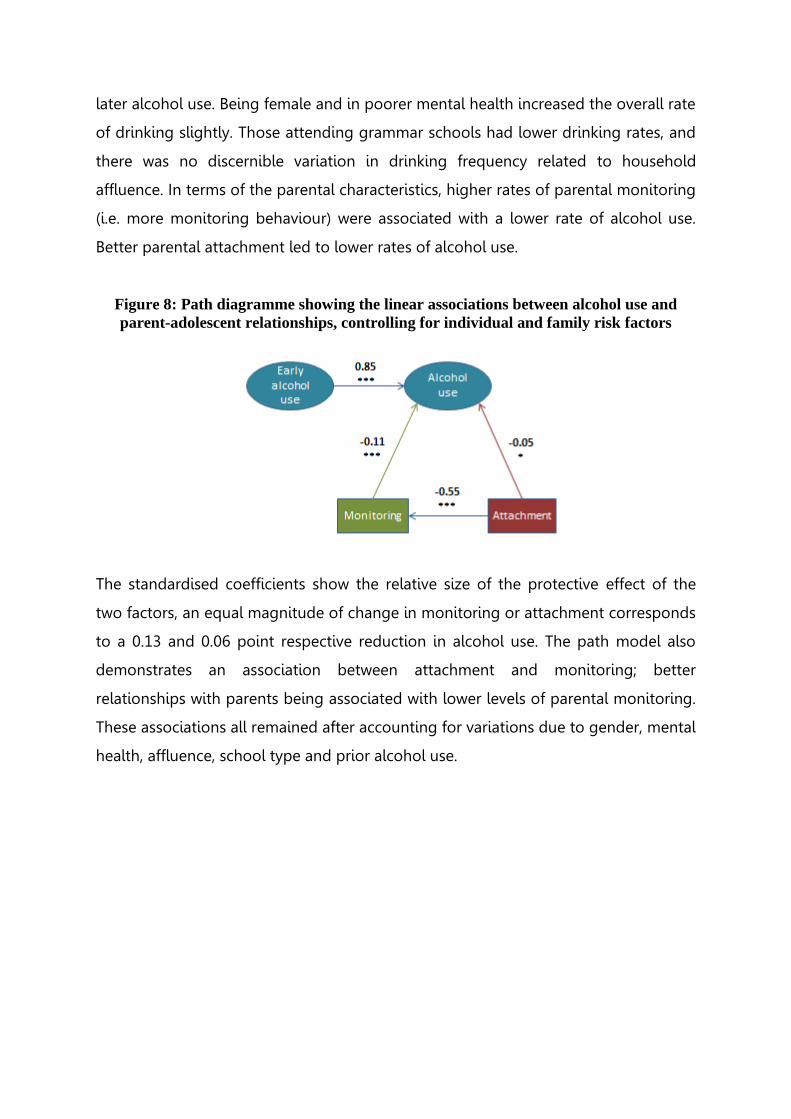
later alcohol use. Being female and in poorer mental health increased the overall rate

of drinking slightly. Those attending grammar schools had lower drinking rates, and

there was no discernible variation in drinking frequency related to household

affluence. In terms of the parental characteristics, higher rates of parental monitoring

(i.e. more monitoring behaviour) were associated with a lower rate of alcohol use.

Better parental attachment led to lower rates of alcohol use.

Figure 8: Path diagramme showing the linear associations between alcohol use and

parent-adolescent relationships, controlling for individual and family risk factors

The standardised coefficients show the relative size of the protective effect of the

two factors, an equal magnitude of change in monitoring or attachment corresponds

to a 0.13 and 0.06 point respective reduction in alcohol use. The path model also

demonstrates an association between attachment and monitoring; better

relationships with parents being associated with lower levels of parental monitoring.

These associations all remained after accounting for variations due to gender, mental

health, affluence, school type and prior alcohol use.

While figure 8 showed the overall model, with simply direct associations between

each variable and alcohol use independent of the influence of the other factors,

Figure 9 shows the how these factors interact with each other and ultimately alcohol

use. The solid lines show the direct associations, higher levels of monitoring lead to

lower levels alcohol use, and better attachment also leads to less alcohol use.

Figure 9: Direct and indirect effects of parental relationship on alcohol use

The dashed line shows the indirect effect of attachment via parental monitoring; in

this case, higher levels of attachment lead to higher rates of alcohol use, and this

increased risk can be explained by the tendency for more securely attached young

people to be less heavily monitored. This lower monitoring thus increases the risk of

drinking. This indirect effect of attachment on alcohol use appears even after

accounting for the effects of gender, mental health, affluence and school type. In

other words, good parental attachment is protective against drinking, but is

simultaneously a risk factor, due to its tendency to reduce parental monitoring.

Figure 10 shows the total effect parameters for this model. Whereas Figure 7 showed

the average effect of attachment after removing the influence of factors such as

monitoring, this model presents the overall effect of different levels of attachment,

including how it affects children’s alcohol use directly; and how it affects monitoring,

the other key driver of alcohol use.

Figure 10: Total effects of parent relationships on alcohol use, accounting for indirect

effects, personal and school characteristics

Table 8: Indirect, direct and overall effect of parental attachment on drinking,

adjusting for various confounders

Model 1 Model 2 Model 3 Model 4 Model 5

Predictors of alcohol use

Monitoring -0.11*** -0.11*** -0.11*** -0.10*** -0.10*** Attachment

Direct effect -0.04* -0.04* -0.03 -0.02 -0.02 Indirect effect via monitoring 0.05*** 0.05*** 0.05*** 0.04*** 0.04***

Total effect 0.01 0.01 0.01 0.02 0.02

Prior alcohol use 0.85*** 0.85*** 0.86*** 0.84*** 0.84*** Gender (Female) -0.03 -0.03 -0.3 -0.03

Mental Health -0.02 -0.02 -0.02 Affluence 0.01 0.001

Grammar school -0.05* -0.07* Lives with:

Biological parents Reference Reconstituted family 0.02*

Single parent 0.01 Effect of attachment on monitoring -0.55 -0.55 -0.55 -0.55 -0.55

Summary of findings

The analysis above assessed the coevolution of alcohol use and parental monitoring;

examined school level variations in alcohol use and overall levels of monitoring,

assessed if differences appeared in the co-evolution of alcohol use and monitoring

in different school contexts, looked to see if there were distinct patterns of parental

monitoring, and finally, examined the interplay between parental monitoring,

parental attachment, and alcohol use.

Monitoring and Alcohol use over time

By looking at survey responses over five years, from ages 11 to 16, we found

evidence of a bi-directional association between frequency of alcohol use and

parental monitoring, weighted towards monitoring being the more important factor.

Young people who were drinking alcohol tended to experience less parental

monitoring in later years, this effect was rather modest, except in the case of those

who had started drinking by age 11. Those reporting early drinking experienced

lower rates of subsequent monitoring; the reducing effect was three times larger

than that occurring in later years. A much stronger association appeared for

monitoring tending to reduce alcohol use, there was a consistent tendency for

higher levels of monitoring leading to lower levels of drinking in the subsequent

survey year. Higher levels of monitoring at an early age had a lasting protective

effect, and were predictive of less frequent drinking right up to age 16.

Three methods by which parents could obtain monitoring information from their

children were assessed in the study, each of these having a different association with

alcohol use. Parental solicitation showed virtually no association with alcohol use.

There was some evidence that more frequent drinkers in the first year of the study

experienced less solicitation in the following year, but there was no evidence of

solicitation influencing alcohol use. Parental control by comparison was very strongly

associated with alcohol use. Respondents whose parents exert greater control over

their free time activities tend to drink less frequently, this was a consistent effect

across time, and early control had a lasting influence on alcohol use. This was a

distinct pattern suggesting alcohol use led to lower levels of parental control. There

was a consistent and long term effect, with higher rates of drinking at early ages

leading to lower control, drinking at age 11 was predictive of control levels at age

16. However, this effect was relatively small by comparison to the effect of control on

alcohol use. Voluntary disclosure of the respondents’ activities to parents was also

associated with lower alcohol use, although this effect tended to reduce at older

ages, to the extent that it appeared unrelated to alcohol use by age 15/16. Alcohol

use was associated with slightly lower rates of disclosure in subsequent years, there

is a slightly larger effect for those drinking at age 11, this again is a marginal effect

by comparison to the effect of disclosure on alcohol use.

The study did not uncover large gender differences, neither in the influence of

monitoring on alcohol use, nor in the tendency for alcohol use to affect monitoring.

There was some suggestion that females experienced a greater protective effect

from monitoring in year 3 in terms of alcohol use in year 4. The lack of consistent

association across the years suggests caution in interpreting a gender difference.

Variation between schools

There was some evidence that there was systematic variation in the rates of drinking

attributable to differences between schools, rather than due to differences between

individuals. The influence of schools was rather small, with school factors accounting

for only 6% of the variation in rates of drinking. Some schools had higher overall

rates of drinking than others; importantly, there were also large differences between

schools in the association between parental monitoring and subsequent alcohol use.

In most schools, parental monitoring was protective against alcohol use, but there

was a great deal of variation, and in some schools there was little to no protective

effect. The protective effect of parental monitoring was not related to overall level of

drinking within the schools. If there was a strong relationship, for example if schools

with low rates of alcohol use were the schools that had less of a protective effect of

monitoring, then this might be evidence of a ‘floor effect’. A floor effect is where the

lack of protective association is due to the low rates of drinking being ‘at the floor’

and thus cannot drop any further. There is no evidence of a floor effect in schools,

hence it appears that something else must explain the change in protective effect of

monitoring. This pattern was the same for all monitoring scales, apart from parental

solicitation which showed no association with alcohol use in the first place. There no

evidence that parental monitoring varied according to the school pupils attended.

There was some evidence that respondents’ peer group influenced their drinking.

Young people who had friends that drank more often were more likely to drink

themselves, even after controlling for their own levels of drinking, while average level

of parental monitoring among friends was not protective against drinking.

After accounting for the individual effect of gender on rates of drinking, and the

influence of other personal and family characteristics, being in a school with a higher

proportion of frequent drinkers was associated with a higher risk of frequent

drinking. Pupils attending girls only schools had elevated rates of drinking compared

to those attending co-educational schools, while boys schools did not differ from co-

educational schools. The effect of parental monitoring did not differ across school

type. There was no difference comparing catholic and state maintained schools.

Attending a school in Ballymena was associated with lower drinking rates, even after

accounting for personal characteristics, and the protective effect of parental

monitoring was weaker in Ballymena than elsewhere, this phenomenon persisted

even after accounting for the fact that Ballymena schools had lower overall rates of

drinking.

Latent profile analyses were used to assess if there were distinct patterns of each

parental monitoring subscales. Results showed that there was no strong evidence

towards selective use of monitoring strategies among the cohort; respondents who

were reported high levels of monitoring on one scale tended to report high values

on all other scales. Statistical tests indicated that the most efficient description of the

patterns in the data was by three groups; low, medium and high monitoring. People

within each group reported high, medium or low levels on all four scales, monitoring,

solicitation, control and disclosure. In the low monitoring group, child disclosure was

on average lower than solicitation or control, and similarly in the high group,

disclosure was higher than the other two.

The final stage of analysis looked at the relationship between monitoring,

attachment and alcohol use. When looked at in isolation, good parental attachment

and higher levels of monitoring both have a protective effect to reduce frequency of

alcohol use. When looking at the inter-relationship between these factors, parental

attachment shows a negligible net effect on alcohol use; this is because parental

attachment simultaneously reduces the likelihood of a young person’s drinking,

while simultaneously reducing the extent to which they are monitored. Lower

monitoring in turn increases their likelihood of drinking.

Discussion

The first phase of analysis set out to describe test two mechanisms to explain the

association between parental monitoring and alcohol use, alcohol affecting

monitoring, and monitoring affecting alcohol use. Firstly, we assessed if higher

monitoring leads to lower rates of alcohol use. The results of the models suggested

that this was indeed the case. Higher monitoring was associated with reduced risk of

frequent alcohol drinking in subsequent years. It also appeared that higher parental

monitoring in year one was associated with lower drinking in years two, three and

five of the study, suggesting that there was a longer term influence of early

parenting styles. Rates of parental monitoring tend to reduce throughout

adolescence. These results suggest that higher than average levels of monitoring, at

any given age, reduces drinking frequency. These results are in agreement with much

of the international literature in the field. The results presented here have the

advantage of showing associations over time, demonstrating both a consistent

protective effect across the early teenage and late pre-teen years, and additionally

the lasting influence of higher parental monitoring at an early age.

Secondly, we assessed if alcohol use influenced levels of parental monitoring. The

models suggested that this was the case, respondents who reported drinking more

frequently tended to report lower levels of parental monitoring in the subsequent

year. Unlike the results for the opposite direction, there was no evidence that more

frequent drinking at an early age had an influence on longer term levels of

monitoring.

These findings are relevant to public health approaches to reducing alcohol use

among young people. Creating higher levels of parental monitoring for parents of

children, in particular encouraging higher parental monitoring around ages 10 – 13

may be an effective method of reducing the frequency of alcohol use throughout

adolescence. Parental monitoring is associated with reducing the risk of other risky

behaviours, suggesting that interventions that can lead to elevated monitoring will

produce broad global benefits, a major caveat of this interpretation would involve

considering the influence of school environment (see below).

Once young people begin using alcohol, this has a tendency to reduce the rates at

which they are monitored. This reverse causal mechanism is important, as there may

be a tendency for children to negotiate parental boundaries in order to facilitate

further drinking. What is not clear from these results is the extent to which these

influences represent children negotiating monitoring behaviour to facilitate drinking,

or alternatively they represent parents’ voluntary reduction in monitoring behaviour

as part of accepting their children’s alcohol use as part of growing up. This effect

appears to be somewhat reversible and potentially transient, as - after adjusting for

background factors - year one drinking is not strongly associated with monitoring in

years two, three, or four. The finding of early alcohol use being associated with less

monitoring at later ages disappears or is greatly attenuated after accounting for

variations due to gender, affluence, parental attachment and living arrangements

(reconstituted families and single parent families faring worse than two biological

parents). This suggests that the majority of this effect is due to shared environmental

features, which reduce parental monitoring and increase early onset drinking

somewhat independently. Despite this finding, the effect did not disappear

altogether, suggesting that parental monitoring is to some extent youth-driven.

Taken in combination with the environmental influences, and the wider body of work

suggesting that these environmental influences also affect parental drinking; these

findings suggest that alcohol use from as early as 11 years old is having a

detrimental effect on family dynamics. The policy implications of this finding are

thus; improved parental monitoring may be appropriate for a ‘risk reducing’

approach for parents of alcohol using children, rather than useful only as a

preventive approach for parents of non-drinking children. However, early drinkers

tend to experience other environmental stressors within the home (deprivation,

change in living arrangements, poorer parental attachment), this would suggest that

any interventions aimed at a ‘risk reducing’ approach will have to contend with the

additional risks posed by deprivation and family discord after effecting change in

monitoring behaviour.

Alongside looking at the overall parental monitoring scale, we assessed the

importance of the source of information about the young person’s activities. Similar

to previous studies (see Stavrinides, Georgiou & Demetriou, 2010), parental solicitation,

the extent to which parents ask about activities or enquire about how a person

spends their free time showed little to no signs of association with alcohol use.

Parental control, the extent to which the young person must seek permission to go

out / visit friends etc. showed a similar pattern as appeared for the overall

monitoring scale. Previous studies have also found that higher control is associated

with lower rates of drinking (Foxcroft & Lowe, 1991).

An additional finding from our results, is the fact that prior alcohol use seems to

have a greater effect to reduce subsequent control behaviours than was found for

the overall monitoring scale, with alcohol use at several ages being associated with

lower rates of parental control by year five.

This supports the idea that adolescents act to exert greater autonomy in order to

facilitate their drinking behaviour.

Greater levels of child disclosure were also associated with less frequent alcohol use.

As with the overall monitoring parental control scales, higher levels at early ages had

a lasting influence on alcohol use throughout the study, with a consistent effect of a

one unit increase in child disclosure leading to a 20% reduction in drinking

frequency. By comparison, the effect of alcohol use on child disclosure is much less

persistent. There is a tendency for drinking in any year to lead to less disclosure in

the subsequent year, but not over the longer term.

The fact that early experience of drinking has a greater influence on the need to

obtain permission from parents than it does overall parental knowledge or child

disclosure indicates that early alcohol use may act as a catalyst to change the

dynamics of the parent-child relationship and how young people relate information

to their parents, rather than alcohol acting to reduce monitoring independently of

the quality of parental relationship.

There was little evidence to suggest that the pattern of associations differed

comparing male and female respondents. Female respondents reported higher levels

of monitoring at all ages and across all subscales. Males also reported drinking more

frequently at all ages. Despite the overall difference between the two groups, the

protective effect of monitoring to reduce drinking does not differ by gender.

Similarly, the effect of prior alcohol use to change subsequent monitoring levels

does not change according to gender. This would suggest interventions aimed at

improving alcohol related outcomes by focussing on improving parental monitoring

should be equally effective for parents of boys as for parents of girls. This should

allow for much easier deployment of interventions, as there is no need to tailor

programmes according to gender.

School variations in alcohol use

With pupils from over 40 schools participating in the study, the BYDS is well suited to

investigating school level influences on alcohol use. The analyses presented here

found that, even after accounting for individual level influences, (gender, prior

alcohol use, parental monitoring etc.) there was a fair amount of difference between

schools in terms of frequency of drinking by year five (around age 16). This has

important implications for public health relating to alcohol use, as it appears that the

school environment plays an important role in shaping young people’s alcohol use.

Besides the overall frequency of drinking varying between schools, there was quite a

large amount of variation in the protective effect of parental monitoring across

schools. On average, a one unit increase in monitoring in year four was associated

with a 30% reduction in drinking rates in the following year. At one extreme (for

schools at the 5th percentile) this effect increased up to a 48% protective effect, while

at the other extreme the effect was only a 7% reduction. This variation between

schools appeared even more marked for year one monitoring, for some schools,

early levels of monitoring were associated with a 47% reduction, while in others

there appeared to be no protective effect whatsoever. A similar pattern appeared for

parental control and child disclosure, in that some schools there was little or no

protective effect. This finding underlines the importance of influences beyond the

parent or family unit. The most likely intervening factor leading to this variation is of

course peer socialisation. In some schools, the influence of peers may be such that

young people are more likely to drink, regardless of the extent to which their

parents’ monitoring aims to prevent them doing so. In other schools, the influence of

peers may be less pronounced, and parents may be better placed to counter the

influences on drinking behaviour.

The fact that the early influence on alcohol use (year 1 to year 5) showed greater

variation than the ‘short-run’ protective effect (year 4 to year 5) is also noteworthy.

This could be due to the difference in the social context of drinking in some schools

compared to others. In schools where social drinking is more common, the early

protective effects may be ‘washed out’ as children may experience more change in

their social behaviours outside the home than for other children where there is less

opportunity for social drinking.

After accounting for individual characteristics (including the gender difference in

drinking rates) pupils attending girls only schools were more likely to drink

frequently than those attending co-educational schools. Pupils attending boys only

schools were no more likely to drink than those attending co-educational schools. By

year five, the proportions of weekly or more frequent drinkers in co-educational,

boys’ and girls’ schools were 42%, 50% and 52% respectively. In co-educational

schools, there was no gender difference in the proportions drinking frequently (42%

for both groups). The protective effect of parental monitoring did not vary by school

gender. These findings again point to the importance of school environment for risk

of drinking. The reason for the elevated risk in girls’ schools is unclear, it certainly

appears that the gender difference in rates of drinking for this cohort of younger

people is negligible. The change in gender roles over the last century has seen a

corresponding increase in alcohol use among women, and the results here attest to

the erosion of the traditional pattern of abstinence from alcohol among women.

Single gender schools have higher overall rates of drinking, after accounting for

confounding factors, the rate remained elevated for girls’ schools. This suggests that

there may be differences in girls’ and boys’ schools in the extent to which factors

such as monitoring affect drinking risk. Girls in co-educational schools are more

heavily monitored than their peers in girls only schools, while boys in boys’ schools

experience less monitoring than boys in co-educational schools. It may be the case

that girls attending co-educational schools are more heavily monitored, perhaps due

to parental concerns surrounding sexual relationships, and this has the protective

effect on alcohol use. Parents of girls attending girls’ schools may have less concern

over sex and pregnancy due to less frequent contact with boys, but this has the

effect of facilitating more frequent drinking.

Pupils attending schools in Ballymena had lower risk of drinking alcohol as

frequently. The protective effect of parental monitoring on alcohol use was also less

pronounced in Ballymena than elsewhere. The demographic profile of Ballymena

contains a large proportion of people from religious groups that traditionally abstain

from alcohol. This may in part account for the lower overall rates and frequency of

alcohol use; however, the tendency for a less protective effect of monitoring in

Ballymena persisted after accounting for the difference in rates of drinking between

schools. This suggests that the difference in peer influences on alcohol use between

Ballymena and Belfast go beyond simple rates of exposure to alcohol. There are

other differences in the environment that make parental influence less important a

protective factor.

Latent profile analyses were used to assess the inter-relationship between the overall

monitoring scale, and the three subscales representing different means of receiving

information about children’s activities. These findings found that all scales correlated

to a large degree, scoring highly on one of the scales was predictive of scoring

highly on all others. The best model predicted three classes, each scoring high,

medium or low on all scales. This finding is important, as it suggests there is some

degree of consistency – at least from a child’s perspective – in the extent to which

parents understand their children’s day to day lives. Were it the case that the scales

demarcated different methods of gaining monitoring information, this would

suggest that there are distinct styles of parenting behaviours in the population, some

of which may be more or less amenable to intervention than others. For example,

had some parents relied exclusively on controlling behaviour, while others relied

solely on soliciting information from children instead of controlling their child’s

activities, an intervention aimed at improving the extent to which children disclose

information about their free time activities might appear completely unsuitable to

these family dynamics. In fact, it appears to be the case that parents rely to a greater

or lesser extent on all three means of monitoring styles, and thus global

improvement in monitoring and communication can improve outcomes for children.

The final stage of analysis looked at the relationship between parental monitoring,

attachment, and alcohol use. The findings were that, in the short term, better

parental attachment did not affect drinking frequency. The underlying reason for this

was more complex. Better parental attachment, independent of other influences,

tends to reduce the amount that young people drink. Better attached children also

tend to be less heavily monitored; this lower monitoring then enables drinking

behaviour and thus acts to increase the risk of drinking. The combination of the

positive and a negative effect on drinking risk, is thus a zero association. On face

value, this finding would suggest that if an intervention wants to reduce alcohol use

among young people, then it would be better focussing on improving parental

monitoring behaviour rather than aiming to improve parent-child attachment. This of

course ignores the complex relationship between parent-child relationship and the

extent to which this can determine monitoring behaviour. It may be impossible to

change monitoring, control, parental solicitation and child disclosure without first

acting to improve the relationships, communication and openness which may

underpin these behaviours. Furthermore, intervening to increase parental monitoring

may lead parents to adopt more authoritarian and controlling behaviours, which may

worsen family relationships without a corresponding improvement in parental

knowledge. Levels of monitoring tend to decrease into later adolescence, with

teenagers exerting greater autonomy and having greater freedom to drink and

engage in other ‘risky’ behaviours. As such, the role of monitoring plays an

increasingly smaller role in outcomes for young people. Quality of relationships, with

parents, other adults, peers and partners do play an important part at all ages, and

the relative importance of these factors is likely to increase. The data reported here

only looked at outcomes around 16 years; it may be the case that in the longer term,

attachment becomes the greater influence on outcomes.

The outcome for this study was frequency of alcohol use, ranging from non-drinking,

infrequent drinkers, monthly drinkers, or weekly or more frequent drinkers. This

outcome measure may not serve as a useful indicator of problematic alcohol use.

There is no indication of drunkenness, amount consumed when drinking, or other

indications of problematic alcohol use, even for those who stated they are drinking

weekly or more frequently. As such, there is a limitation on the extent to which these

results demonstrate school variation, or protective family level factors in terms of

‘risky’ or harmful alcohol use. Further studies should assess the extent to which the

parenting and family characteristics identified here are related to longer term

indicators of harmful drinking. The major strength of the approach used here is that

the measure of alcohol use, while less indicative of longer term problems, was

equally applicable at all ages in the study. Measure such as expenditure on alcohol,

or Alcohol Use Disorders Identification Test scores would not be applicable to 11

year olds in the same way as they are for 18 year olds. By using a less specific

measure of alcohol problems, the study was more sensitive to less dramatic changes

in the development of alcohol behaviours; the results were able to demonstrate the

relationship between monitoring and alcohol use throughout the early teenage years

across a time period when both behaviours are changing. Furthermore, drinking

alcohol once a week or more frequently below age 16 is a risk factor for longer term

negative health outcomes.

The findings of this study are of importance to the academic understanding of

adolescent development and alcohol use, and to the field of alcohol harm reduction,

family support, and youth alcohol policy.

The scale of this study makes it rather exceptional in the study of the interaction

between adolescent and family behaviour; it is the size of this study that allowed us

to uncover both environment-driven, and youth-driven influences of greater alcohol

use being followed by lower monitoring, making an important contribution to the

current understanding of the monitoring – child behaviour literature.

The ability to investigate between school differences underlines the importance of

the wider context of alcohol use beyond the influence of the family. Any attempt to

improve alcohol outcomes must take into account how the relative influence of

parents and peers changes with age.

Lastly, these findings have demonstrated how policies or practices which target a

single aspect of social functioning are likely to be inadequate in achieving improved

outcomes for young people. Influencing one aspect of family functioning will have

knock-on consequences for other aspects of family life and subsequent adolescent

outcomes, and all of these influences are further limited depending on the relative

influence of school and peer environments.

These findings may have resonance for policy and practice surrounding young

people’s use of alcohol, family environment and school environment. While we have

highlighted some of these issues, further work is needed to communicate these

findings to stakeholders, gain feedback on the implications, and find ways in which

the public response to alcohol related harms can change.

References

Anderson, A.R. & Henry, C.S. (1994). Family system characteristics and parental behaviors as predictors of adolescent substance use. Adolescence, 29, 405-420. Andrews, J.A., Tildesley, E., Hops, H. & Li, F. (2002). The influence of peers on young adult substance use. Health Psychology, 21 (4), 349-357. Arata, C.M., Stafford, J. & Tims, M.S. (2003). High school drinking and its consequences. Adolescence, 38, 151, 567-79.

Armsden, GC. & Greenberg, MT. "The inventory of parent and peer attachment: Individual differences and their relationship to psychological well-being in adolescence." Journal of youth and adolescence 16.5 (1987): 427-454.

Ary, D.V., Duncan, T.E., Biglan, A., Metzler, C.W., Noell, J.W. & Smolkowksi, K. (1999). Development of Adolescent Problem Behavior. Journal of Abnormal Child Psychology, 27 (2), 141-150. Bahr, S.J., Hoffmann, J.P. & Yang, X. (2005). Parental and Peer Influences on the Risk of Adolescent Drug Use. The Journal of Primary Prevention, 26 (6), 529-551.

Balsa, A.I., Giuliano, L.M., French, M.T. (2011). The effects of alcohol use on academic achievement in high school. Economics of Education Review, 30 (1), 1-15.

Barnes, G.M. & Farrell, M.P. (1992). Parental Support and Control as Predictors of Adolescent Drinking, Delinquency, and Related Problem Behaviours. Journal of Marriage and the Family, 763-776. Barnes, G.M., Hoffman, J.H., Welte, J.W., Farrell, M.P. & Dintcheff, B.A. (2006). Effects of Parental Monitoring and Peer Deviance on Substance Use and Delinquency. Journal of Marriage and Family, 68 (4), 1084-1104. Barnes, G.M., Reifman, A.S., Farrell, M.P. and Dintcheff, B.A. (2000). The Effects of Parenting on the Development of Adolescent Alcohol Misuse: A Six-Wave Latent Growth Model. Journal of Marriage and Family, 62(1), 175-186. Barry, A.E., Chaney, B. & Chaney, J.D. (2011). The Impact of Truant and Alcohol-Related Behavior on Educational Aspirations: A Study of US High School Seniors. The Journal of School Health, 81 (8), 485-492. Bergh, D., Hagquist, C. & Starrin, B. (2011). Parental Monitoring, Peer Activities and Alcohol Use: A Study Based on Data on Swedish Adolescents. Drugs: Education, Prevention & Policy, 18 (2), 100-107. Bernburg, J.G., Thorlindsson, T. and Sigfusdottir, I.D. (2009). The neighborhood effects of disrupted family processes on adolescent substance use. Social science & medicine, 69(1), 129-137.

Borawski, E.A., Ievers-Landis, C.E., Lovegreen, L.D. & Trapl, E.S. (2003). Parental Monitoring, Negotiated Unsupervised Time, and Parental Trust: The Role of Perceived Parenting Practices in Adolescent Health Risk Behaviors. Journal of Adolescent Health, 33, 60-70. Borsari, B. and Carey, K.B. (2001). Peer influences on college drinking: A review of the research. Journal of substance abuse, 13(4), 391-424. Bränström, R., Sjöström, E. & Andréasson, S (2007). Individual, group and community risk and protective factors for alcohol and drug use among Swedish adolescents. European Journal of Public Health, 18 (1):12-8. Bremner, P., Burnett, J., Nunney, F., Ravat, M. & Mistral, W. (2011). Young people, alcohol and influences. A study of young people and their relationship with alcohol. York: Joseph Rowntree Foundation.

Capaldi, D.M. & Stoolmiller, M., Kim, H.K. & Yoerger, K. (2009). Growth in alcohol use in at-risk adolescent boys: Two-part random effects prediction models. Drug and Alcohol Dependence, 105, 109-117. Cavazos-Rehg, P.A., Spitznagel, E.L., Bucholz, K.K., Nurnberger, J., Edenberg, H.J., Kramer, J.R., Kuperman, S., Hesselbrock, V., Bierut, L.J. (2010). Predictors of Sexual Debut at Age 16 or Younger. Archives of Sexual Behaviour, 39(3), 664-673.

Clark, A.E. & Loheac, Y. (2007). “It wasn’t me, it was them!” Social influence in risky behavior by adolescents. Journal of Health Economics, 26, 763-784. Cleveland, M.J., Feinberg, M.E. & Greenberg, M.T. (2010). Protective families in high- and low-risk environments: implications for adolescent substance use. Journal of Youth and Adolescence, 39, 114-126. Cleveland, M.J., Feinberg, M.E., Osgood, W. & Moody, J. (2012). Do Peers’ Parents Matter? A New Link Between Positive Parenting and Adolescent Substance Use. Journal of Studies on Alcohol and Drugs, 73, 423-433.

Cleveland, M.J., Gibbons, F.X., Brody, G.H., Gerrard, M. & Pomery, E.A. (2005). The Impact of Parenting on Risk Cognitions and Risk Behavior: A Study of Mediation and Moderation in a Panel of African American Adolescents. Child Development, 76 (4), 900-916.

Cohen, D.A., Richardson, J. & LaBree, L. (1994). Parenting Behaviors and the Onset of Smoking and Alcohol Use: A Longitudinal Study. Pediatrics, 94 (3), 368-375. De Haan, L. & Boljevac, T. (2009). Alcohol Use Among Rural Middle School Students: Adolescents, Parents, Teachers and Community Leaders’ Perceptions. Journal of School Health, 79, 2, 59-66. Dick, D.M., Pagan, J.L., Holliday, C., Viken, R., Pulkkinen, L., Kaprio, J. & Rose, R.J. (2007). Gender Differences in Friends’ Influences on Adolescent Drinking: A Genetic Epidemiological Study. Alcoholism: Clinical and Experimental Research, 31 (12), 2012-2019.

Dickens, D.D., Dieterich, S.E., Henry, K.L. & Beauvais, F. (2012). School Bonding As a Moderator of the Effect of Peer Influences on Alcohol Use Among American Indian Adolescents. Journal of Studies on Alcohol and Drugs, 73, 597-603. Dishion, T.J., and McMahon, R.J. (1998). Parental monitoring and the prevention of child and adolescent problem behavior: A conceptual and empirical formulation. Clinical child and family psychology review, 1(1), 61. Dishion, T.J. and Owen, L.D. (2002). A longitudinal analysis of friendships and substance use: Bidirectional influence from adolescence to adulthood. Developmental psychology, 38(4), 480. Donath, C., Grabel, E., Baier, D., Pfeiffer, C., Karagulle, D., Bleich, S. & Hillemacher, T. (2011). Alcohol consumption and binge drinking in adolescents: comparison of different migration backgrounds and rural vs. urban residence-a representative study. BMC Public Health, 11: 84. DOI:10.1186/1471-2458-11-84. Donovan, J.E., Leech, S.L., Zucker, R.A., Loveland-Cherry, C.J., Jester, J.M., Fitzgerald, H.E., Puttler, L.I., Wong, M.M. & Looman, W.S. (2004). Really underage drinkers: alcohol use among elementary students. Alcoholism: Clinical and Experimental Research, 28, 2, 341-349. Duncan, S.C., Duncan, T.E., Biglan, A. & Ary, D. (1998). Contributions of the social context to the development of adolescent substance use: a multivariate latent growth modeling approach. Drug and Alcohol Dependence, 50, 57-71.

Ellickson, P.L. Tucker, J.S., Klein, D.J. (2003). Ten-year prospective study of public health problems associated with early drinking. Pediatrics, 111: 949-55.

Felson, R.B., Teasdale, B. & Burchfield, K.B. (2008). The influence of being under the influence: Alcohol effects on adolescent violence. Journal of Research in Crime and Delinquency, 45 (2), 119-141. Fergusson, D.M. & Lynskey, M.T. (1996). Alcohol misuse and adolescent sexual behaviors and risk taking. Pediatrics, 98:91-6. Finkenauer, C., Engels, R. C. M. E., & Meeus, W. (2002). Keeping secrets from parents: Advantages and disadvantages of secrecy in adolescence. Journal of youth and adolescence, 31(2), 123. Fletcher, J.M. (2012). Peer influences on adolescent alcohol consumption: evidence using an instrumental variables/fixed effect approach. Journal of population economics, 25, 4, 1265-1286. Fosco, G.M., Stormshak, E.A., Dishion, T.J. & Winter, C.E. (2012). Family relationships and parental monitoring during middle school as predictors of early adolescent problem behavior. Journal of Clinical Child & Adolescent Psychology, 41 (2), 202-13. Foxcroft, D.R. & Lowe, G. (1991). Adolescent drinking behavior and family socialization factors: a meta-analysis. Journal of Adolescence, 14 (3), 255-273. Gaughan, M. (2006). The Gender Structure of Adolescent Peer Influence on Drinking. Journal of Health and Social Behavior, 47 (1), 47-61.

Goodman, A., Hurcombe, R., Healy, J., Goodman, S & Ball, E. (2011). Teenage drinking and interethnic friendships. York: Joseph Rowntree Foundation. Gossrau-Breen, D., Kuntsche, E. & Gmel, G. (2010). My older sibling was drunk- Younger siblings’ drunkenness in relation to parental monitoring and the parent-adolescent relationship. Journal of Adolescence, 33, 643-652. Gottfredson, M. and Hirschi, T. (1990). A general theory of crime. Stanford, Calif.: Stanford University Press. Gottfredson, N.C. & Hussong, A.M. (2011). Parental involvement protects against self-medication behaviors during the high school transition. Addictive Behaviors, 36, 1246-1252. Griffin, K.W., Botvin, G.J. Scheier, L.M., Diaz, T. & Miller, N.L. (2000). Parenting practices as predictors of substance use, delinquency and aggression among urban minority youth: Moderating effects of family structure and gender. Psychology of Addictive Behaviors, 14 (2), 174-184. Habib, C., Santoro, J., Kremer, P., Toumbourou, J., Leslie, E. & Williams, J. (2010). The importance of family management, closeness with father and family structure in early adolescent alcohol use. Addiction, 105, 1750-1758. Henry, K.L., Oetting, E.R. & Slater, M.D. (2009). The Role of Attachment to Family, School, and Peers in Adolescents’ Use of Alcohol: A Longitudinal Study of Within-Person and Between-Persons Effects. Journal of Counseling Psychology, 56 (4), 564-572.

Jimenez-Iglesias, A., Moreno, C., Rivera, F. & Garcia-Moya, I. (2013). The role of the family in promoting responsible substance use in adolescence. Journal of Child and Family Studies, 1062-1024.

Keijsers, L., Frijns, T., Branke, S.J.T., and Meeus, W. (2009). Developmental links of adolescent disclosure, parental solicitation, and control with delinquency: Moderation by parental support. Developmental psychology, 45(5), 1314. Kelly, A.B., O’Flaherty, M., Toumbourou, J.W., Connor, J.P., Hemphill, S.A., and Catalano, R.F. (2011). Gender differences in the impact of families on alcohol use: a lagged longitudinal study of early adolescents. Addiction, 106(8), 1427-1436. Kerr, M. & Stattin, H. (2000). What Parents Know, How They Know It, and Several Forms of Adolescent Adjustment: Further Support for a Reinterpretation of Monitoring. Developmental Psychology, 36 (3), 366-380. Kerr, M., Stattin, H. and Burk, W.J. (2010). A Reinterpretation of Parental Monitoring in Longitudinal Perspective. Journal of Research on Adolescence, 20(1), 39-64. Kim, Y. & Neff, J.A. (2010). Direct and indirect effects of parental influence upon adolescent alcohol use: A structural equation modeling analysis. Journal of Child & Adolescent Substance Abuse, 19 (3), 244-260.

Kuntsche, E. and Jordan, M.D. (2006). Adolescent alcohol and cannabis use in relation to peer and school factors: Results of multilevel analyses. Drug and alcohol dependence, 84(2), 167-174. Latendresse, S.J., Rose, R.J., Viken, R.J., Pulkkinen, L., Kaprio, J. & Dick, D.M. (2008). Parenting mechanisms in links between parents’ and adolescents’ alcohol use behaviors. Alcoholism: Clinical and Experimental Research, 32 (2): 322-30. Ledoux, S., Miller, P., Choquet, M. & Plant, M. (2002). Family Structure, Parent-Child Relationships, and Alcohol and Other Drug Use Among Teenagers in France and the United Kingdom. Alcohol & Alcoholism, 37 (1), 52-60. Lundborg, P. (2006). Having the wrong friends? Peer effects in adolescent substance use. Journal of Health Economics, 25, 214-233. Marsden, J., Boys, A., Farrell, M., Stillwell, G., Hutchings, K., Hillebrand, J. & Griffiths, P. (2005). Personal and Social Correlates of Alcohol Consumption among Mid-Adolescents. British Journal of Developmental Psychology, 23 (3), 427-450. Martino, S.C., Ellickson, P.L. & McCaffrey, D.F. (2009). Multiple trajectories of peer and parental influence and their association with the development of adolescent heavy drinking. Addictive Behaviors, 34, 693-700. McKay, M.T., Sumnall, H., Goudie, A.J., Field, M., Cole, J.C. (2010). What differentiates adolescent problematic drinkers from their peers? Results from a cross-sectional study in Northern Irish school children. Drugs: education, prevention and policy, 18 (3), 187-199. Mrug, S., Gaines, J., Su, W. & Windle, M. (2010). School-level substance use: effects on early adolescents’ alcohol, tobacco, and marijuana use. Journal of Studies on Alcohol & Drugs, 71 (4), 488-95. Nash, S.G., McQueen, A. and Bray, J.H. (2005). Pathways to adolescent alcohol use: family environment, peer influence, and parental expectations. Journal of Adolescent Health, 37(1), 19-28. Patock-Peckham, J.A., King, K.M., Morgan-Lopez, A.A., Ulloa, E.C. & Moses, J.M.F. (2011). Gender-Specific Mediational Links Between Parenting Styles, Parental Monitoring, Impulsiveness, Drinking Control and Alcohol-Related Problems. Journal of Studies on Alcohol and Drugs, 72 (2), 247-258.

Peleg-Oren, N., Saint-Jean, G., Cardenas, G.A., Tammara, H. & Pierre, C. (2009). Drinking Alcohol before Age 13 and Negative Outcomes in Late Adolescence 1 Source: Alcoholism-Clinical and Experimental Research, 33(11), 1966-1972. Piko, B.F. & Kovács, E. (2010). Do parents and school matter? Protective factors for adolescent substance use. Addictive Behaviors, 35 (1), 53-6. Pokhrel, P., Unger, J.B., Wagner, K.D., Ritt-Olson, A. & Sussman, S. (2008). Effects of parental monitoring, parent-child communication, and parents’ expectation of the child’s acculturation on the substance use behaviours of urban, Hispanic adolescents. Journal of Ethnicity in Substance Abuse, 7 (2), 200-13.

Rai, A.A., Stanton, B., WU., Y., LI, X., Galbraith, J., Cottrell, L., Pack, R., Harris, C., D’Allessandri, D. & Burns, J. (2003). Relative influences of perceived parental monitoring and perceived peer involvement on adolescent risk behaviors: An analysis of six cross-sectional data sets. Journal of Adolescent Health, 33, 108-118. Rawana, J.S. & Ames, M.E. (2012). Protective Predictors of Alcohol Use Trajectories Among Canadian Aboriginal Youth. Journal of Youth and Adolescence, 41 (2), 229-243. Rehm, J., Monga, N., Adlaf, E., Taylor, B., Bondy, S.J. & Fallu, J.S. (2005). School matters: drinking dimensions and their effects on alcohol-related problems among Ontario secondary school students. Alcohol & Alcoholism, 40(6): 569-74. Ryan, S.M., Jorm, A.F. & Lubman, D.I. (2010). Parenting factors associated with reduced adolescent alcohol use: a systematic review of longitudinal studies. Australian and New Zealand Journal of Psychiatry, 44 (9), 774-783. Schinke, S.P., Fang, L. & Cole, K.C.A. (2008). Substance Use Among Early Adolescent Girls: Risk and Protective Factors. Journal of Adolescent Health, 43, 191-194. Shortt, A.L., Hutchinson, D.M., Chapman, R. & Toumbourou, J.W. (2007). Family, school, peer and individual influences on early adolescent alcohol use: first-year impact of the Resilient Families programme. Drug and Alcohol Review, 26 (6), 625-634. Simons-Morton, B. (2004). Prospective association of peer influence, school engagement, drinking expectancies, and parent expectations with drinking initiation among sixth graders. Addictive Behaviors, 29, 299-309. Simons-Morton, B. & Chen, R. (2005). Latent Growth Curve Analyses of Parent Influences on Drinking Progression among Early Adolescents. Journal of Studies on Alcohol, 66, 5-13. Simons-Morton, B.G., Crump, A.D., Haynie, D.L. & Saylor, K.E. (1999). Student-school bonding and adolescent problem behavior. Health Education Research, 14 (1), 99-107. Simons-Morton, B., Haynie, D.L., Crump, A.D., Eitel, P. & Saylor, K.E. (2001). Peer and parent influences on smoking and drinking among early adolescents. Health Education & Behavior, 28, 95-107. Smit, E., Verdurmen, J., Monshouwer, K. and Smit, F. (2008). Family interventions and their effect on adolescent alcohol use in general populations; a meta-analysis of randomized controlled trials. Drug and alcohol dependence, 97(3), 195-206. Soenens, B., Vansteenkiste, M., Luyckx, K. & Goossens, L. (2006). Parenting and Adolescent Problem Behavior: An Integrated Model With Adolescent Self-Disclosure and Perceived Parental Knowledge as Intervening Variables. Developmental Psychology, 42 (2), 305-318. Sokol-Katz, J., Dunham, R. & Zimmerman, R. (1997). Family structure versus parental attachment in controlling adolescent deviant behavior: a social control model. Adolescence, 32, 199-215. Sondhi, A. & Turner, C. (2011). The influence of family and friends on young people’s drinking. York: Joseph Rowntree Foundation.

Stattin, H. and Kerr, M. (2000). Parental Monitoring: A Reinterpretation. Child development, 71(4), 1072-1085.

Stavrinides, P., Georgiou, S. & Demetriou, A. (2010). Longitudinal associations between adolescent alcohol use and parents’ sources of knowledge. British Journal of Developmental Psychology, 28, 643-655.

Stice, E., Barrera, M. & Chassin, L. (1993). Relation of parental support and control to adolescents’ externalizing symptomatology and substance use: A longitudinal examination of curvilinear effects. Journal of Abnormal Child Psychology, 21 (6), 609-629. Stock, C., Ejstrud, B., Vinther-Larsen, M., Schlattmann, P., Curtis, T., Groenbaek, M. & Bloomfield, K. (2011). Effects of school district factors on alcohol consumption: results of a multi-level analysis among Danish adolescents. European Journal of Public Health, 21, 4, 449-455.

Stoolmiller, M., Wills T.A., McClure, A.C., Tanski, S.E., Worth, K.A., Gerrard, M. & Sargent, J.D. (2012). Comparing media and family predictors of alcohol use: a cohort study of US adolescents. BMJ Open, 2:e000543 doi: 10.1136/bmjopen-2011-000543.

Trucco, E.M., Colder, C.R. & Wieczorek, W.F. (2011). Vulnerability to peer influence: A moderated mediation study of early adolescent alcohol use initiation. Addictive Behaviors, 36, 729-736. Tobler, A.L. & Komro, K.A. (2010). Trajectories or Parental Monitoring and Communication and Effects on Drug Use Among Urban Young Adolescents. Journal of Adolescent Health, 46, 560-568. van der Vorst, H., Engels, R.C.M.E., Meeus, W., Dekovic, M., Vermulst, A. (2006). Parental Attachment, Parental Control, and Early Development of Alcohol Use: A Longitudinal Study. Psychology of Addictive Behaviors, 20 (2), 107-116. Velleman, R. (2009). Children, young people and alcohol: how they learn and how to prevent excessive use. York: Joseph Rowntree Foundation. Velleman, R.D.B., Templeton, L.J. & Copello, A.G. (2005). The role of the family in preventing and intervening with substance use and misuse: a comprehensive review of family interventions, with a focus on young people. Drug and Alcohol Review, 24, 93-109.

Waizenhofer, R.N., Buchanan, C.M. & Jackson-Newsom, J. (2004). Mothers’ and Fathers’ Knowledge of Adolescents’ Daily Activities: Its Sources and Its links with Adolescent Adjustment. Journal of Family Psychology, 18 (2), 348-360. Windle, M. (2000). Parental, Sibling, and Peer Influences on Adolescent Substance Use and Alcohol Problems. Applied Developmental Science, 4, 98-110. Wood, M.D., Read, J.P., Mitchell, R.E. & Brand, N.H. (2004). Do Parents Still Matter? Parent and Peer Influences on Alcohol Involvement Among Recent High School Graduates. Psychology of Addictive Behaviors, 18 (1), 19-30.

Yeh, M., Chiang, I. & Huang, S. (2006). Gender differences in predictors of drinking behavior in adolescents. Addictive Behaviors, 31, 1929-1938.

Appendix 1 Statistical Output for Models Included in the Report

This appendix reports the results of models analysed using Mplus, as described in text and in

diagrams in phase 1 and 2 of the analysis above.

Model 55: Associations between Alcohol use and Parental Monitoring

Year 5 Alcohol Use Odds Ratio P Value Year 1 Monitoring 0.796 <0.001 Year 4 Monitoring 0.746 0.002 Year 4 Alcohol Use 5.027 <0.001

Year 4 Parental Attachment 0.896 0.079

Year 4 Alcohol Use Year 1 Monitoring 0.878 0.037 Year 2 Monitoring 0.837 0.036 Year 3 Monitoring 0.71 <0.001 Year 3 Alcohol Use 3.405 <0.001

Female 1.264 0.013 Year 1 Sdq 1.016 0.776

Year 3 Affluence 1.028 0.45 Year 3 Parental

Attachment 0.906 0.031 Reconstituted

Family 1.645 0.04 Single Parent 1.359 0.037

Year 3 Alcohol Use Year 1 Monitoring 0.842 0.004 Year 2 Monitoring 0.796 <0.001 Year 2 Alcohol Use 3.281 <0.001

Year 2 Affluence 1.089 0.055 Single Parent 1.455 0.006

Year 2 Alcohol Use Year 1 Monitoring 0.732 <0.001 Year 1 Alcohol Use 3.098 <0.001

Female 1.205 0.076 Year 2 Affluence 1.101 0.004 Year 1 Parental

Attachment 1.065 0.118 Reconstituted

Family 1.524 0.011 Single Parent 1.357 0.007

Year 5 Monitoring Linear Regression

Coefficient P Value Year 2 Alcohol Use -0.034 0.065 Year 4 Monitoring 0.548 <0.001

Female 0.087 0.016 Year 4 Sdq -0.041 0.094

Year 4 Parental Attachment -0.15 <0.001

Reconstituted Family -0.232 <0.001

Year 4 Monitoring Year 1 Alcohol Use -0.052 0.047 Year 3 Alcohol Use -0.051 0.022 Year 3 Monitoring 0.626 <0.001

Female 0.108 0.024 Year 1 Sdq -0.036 0.01

Year 3 Affluence 0.021 0.078 Year 3 Parental

Attachment -0.069 0.021 Year 3 Monitoring Year 1 Alcohol Use -0.049 0.062 Year 2 Alcohol Use -0.071 0.002 Year 2 Monitoring 0.553 <0.001

Year 1 Parental Attachment -0.123 <0.001

Year 2 Monitoring Year 1 Alcohol Use -0.143 <0.001 Year 1 Monitoring 0.494 <0.001 Year 1 Affluence 0.027 0.064 Year 1 Parental

Attachment -0.136 <0.001 Reconstituted

Family -0.189 0.005 Single Parent -0.12 0.029

Ssbic

Log Likelihood Correction Factor Free Parameters

Model 65: Alcohol Use and Child Disclosure

Year 5 Alcohol Use Odds Ratio P Value Year 1 Disclosure 0.806 <0.001

Year 4 Alcohol Use 5.608 <0.001 Reconstituted

Family 1.429 0.017 Year 4 Alcohol Use Year 2 Disclosure 0.849 0.004 Year 3 Disclosure 0.645 <0.001

Year 3 Alcohol Use 3.489 <0.001 Female 1.214 0.031

Year 1 Sdq 1.058 0.296 Year 3 Parental

Attachment 0.869 0.004 Reconstituted

Family 1.584 0.062 Single Parent 1.306 0.046

Year 3 Alcohol Use Year 1 Disclosure 0.849 0.006 Year 2 Disclosure 0.785 <0.001

Year 2 Alcohol Use 3.203 <0.001 Year 2 Affluence 1.093 0.039

Reconstituted Family 1.391 0.074

Single Parent 1.537 0.002 Year 2 Alcohol Use Year 1 Disclosure 0.659 <0.001

Year 1 Alcohol Use 2.91 <0.001 Female 1.236 0.038

Reconstituted Family 1.415 0.044

Single Parent 1.369 0.004

Year 5 Disclosure

Linear Regression Coefficient P Value

Year 4 Disclosure 0.561 <0.001 Female 0.126 <0.001

Year 4 Parental Attachment -0.189 <0.001

Reconstituted Family -0.207 0.019

Year 4 Disclosure Year 1 Alcohol Use -0.043 0.108 Year 3 Alcohol Use -0.098 <0.001 Year 3 Disclosure 0.514 <0.001

Female 0.107 0.024 Year 1 Sdq -0.027 0.078

Year 3 Affluence 0.02 0.021 Year 3 Parental

Attachment -0.16 <0.001 Year 3 Disclosure

Year 2 Alcohol Use -0.085 <0.001 Year 2 Disclosure 0.485 <0.001

Female 0.079 0.014 Year 1 Parental

Attachment -0.136 <0.001 Reconstituted

Family -0.157 0.006 Single Parent -0.075 0.151

Year 2 Disclosure Year 1 Alcohol Use -0.13 <0.001 Year 1 Disclosure 0.418 <0.001 Year 1 Affluence 0.051 0.001 Year 1 Parental

Attachment -0.173 <0.001 Reconstituted

Family -0.133 0.053

Ssbic 37778.678

Log Likelihood -18740.642 Correction Factor 1.436 Free Parameters 67

Model 75: Alcohol Use and Parental Control

Year 5 Alcohol Use Odds Ratio P Value Year 3 Control 0.742 0.001

Year 4 Alcohol Use 5.369 <0.001 Year 4 Sdq 1.123 0.033

Year 4 Alcohol Use Year 1 Control 0.828 0.002 Year 2 Control 0.862 0.019 Year 3 Control 0.849 0.01

Year 3 Alcohol Use 3.671 <0.001 Female 1.274 0.008

Year 1 Sdq 1.104 0.058 Reconstituted

Family 1.56 0.074 Year 3 Alcohol Use

Year 1 Control 0.89 0.017 Year 2 Control 0.834 <0.001

Year 2 Alcohol Use 3.413 <0.001 Year 2 Affluence 1.092 0.021 Year 1 Parental

Attachment 1.137 0.02 Reconstituted

Family 1.385 0.084 Single Parent 1.467 0.003

Year 2 Alcohol Use Year 1 Control 0.746 <0.001

Year 1 Alcohol Use 3.039 <0.001 Female 1.233 0.034

Year 1 Parental Attachment 1.157 <0.001

Reconstituted Family 1.431 0.057

Single Parent 1.324 0.014

Year 5 Control

Linear Regression Coefficient P Value

Year 2 Alcohol Use -0.039 0.076 Year 4 Alcohol Use -0.072 0.001

Year 4 Control 0.571 <0.001 Female 0.198 <0.001

Year 4 Control Year 3 Alcohol Use -0.097 <0.001

Year 3 Control 0.516 <0.001 Female 0.301 <0.001

Year 1 Sdq -0.011 0.582 Year 3 Affluence 0.04 0.007 Year 3 Control

Year 1 Alcohol Use -0.065 0.018 Year 2 Alcohol Use -0.072 0.001

Year 2 Control 0.479 <0.001 Female 0.079 0.016

Year 1 Sdq 0.027 0.167 Year 1 Parental

Attachment -0.076 <0.001 Reconstituted

Family -0.197 0.005 Year 2 Control

Year 1 Alcohol Use -0.096 0.005 Year 1 Control 0.45 <0.001

Female 0.144 0.012 Year 1 Sdq 0.04 0.041

Year 1 Affluence 0.036 0.022 Year 1 Parental

Attachment -0.102 <0.001 Reconstituted

Family -0.149 0.015 Single Parent -0.138 0.02

Ssbic 38902.604

Log Likelihood -19381.302 Correction Factor 1.578 Free Parameters 70

Model 85 – Parental Solicitation

Year 5 Alcohol Use Odds Ratio P Value Year 4 Alcohol Use 5.639 <0.001 Year 4 Alcohol Use Year 2 Solicitation 1.021 0.607 Year 3 Alcohol Use 3.963 <0.001

Year 1 Sdq 1.115 0.043 Reconstituted

Family 1.857 0.011 Single Parent 1.35 0.027

Year 3 Alcohol Use Year 2 Alcohol Use 3.523 <0.001

Year 3 Affluence 1.063 0.051 Year 3 Parental

Attachment 1.35 <0.001 Year 2 Alcohol Use Year 1 Alcohol Use 3.351 <0.001

Year 1 Parental Attachment 1.196 <0.001

Reconstituted Family 1.526 0.012

Single Parent 1.287 0.022

Year 5 Solicitation

Linear Regression Coefficient P Value

Year 4 Solicitation 0.549 <0.001 Female 0.149 <0.001

Year 4 Parental Attachment -0.115 <0.001

Reconstituted Family -0.058 0.44

Single Parent -0.031 0.571 Year 4 Solicitation Year 3 Solicitation 0.484 <0.001

Female 0.243 <0.001 Year 3 Affluence 0.043 <0.001 Year 3 Parental

Attachment -0.13 <0.001 Year 3 Solicitation Year 2 Solicitation 0.408 <0.001

Female 0.174 <0.001 Year 2 Affluence 0.022 0.069 Year 1 Parental

Attachment -0.124 <0.001 Year 2 Solicitation Year 1 Solicitation 0.306 <0.001 Year 1 Alcohol Use -0.102 0.001

Female 0.179 <0.001 Year 1 Parental

Attachment -0.164 <0.001 Reconstituted

Family -0.227 0.01 Single Parent -0.133 0.026

Ssbic 39889.550

Log Likelihood -19822.002 Correction Factor 1.646 Free Parameters 55

Gender Interaction Models:

Model 56: Gender Difference in Alcohol use and Parental Monitoring

Year 5 Alcohol Use Odds Ratio P Value Year 1 Monitoring 0.805 0.003 Year 4 Monitoring 0.776 0.032 Year 4 Alcohol Use 4.869 <0.001

Female 0.958 0.793 Female * Year 4

Monitoring 1.094 0.536 Female * Year 1

Monitoring 1.022 0.871 Year 4 Alcohol Use Year 1 Monitoring 0.807 0.01 Year 2 Monitoring 0.787 0.065 Year 3 Monitoring 0.906 0.272 Year 3 Alcohol Use 3.4 <0.001

Female 1.273 0.017 Female * Year 1

Monitoring 1.241 0.072 Female * Year 2

Monitoring 1.08 0.635 Female * Year 3

Monitoring 0.736 0.015 Year 3 Alcohol Use Year 1 Monitoring 0.813 0.008 Year 2 Monitoring 0.826 0.003 Year 2 Alcohol Use 3.352 <0.001

Female 1.18 0.091 Female * Year 1

Monitoring 1.123 0.271 Female * Year 2

Monitoring 0.904 0.371 Year 2 Alcohol Use Year 1 Monitoring 0.783 0.006 Year 1 Alcohol Use 3.228 <0.001

Female 1.23 0.046 Female * Year 1

Monitoring 0.938 0.521

Year 5 Monitoring

Linear Regression Coefficient P Value

Year 2 Alcohol Use -0.049 0.069 Year 4 Monitoring 0.647 <0.001

Female 0.067 0.217 Female * Year 2

Alcohol Use 0.012 0.697 Year 4 Monitoring Year 1 Alcohol Use -0.047 0.108 Year 3 Alcohol Use -0.013 0.639 Year 3 Monitoring 0.664 <0.001

Female 0.199 0.002 Female * Year 1

Alcohol Use -0.012 0.819 Female * Year 3

Alcohol Use -0.06 0.114 Year 3 Monitoring Year 1 Alcohol Use -0.082 0.014 Year 2 Alcohol Use -0.039 0.197 Year 2 Monitoring 0.592 <0.001

Female 0.007 0.921 Female * Year 1

Alcohol Use -0.007 0.911 Female * Year 2

Alcohol Use -0.039 0.253 Year 2 Monitoring Year 1 Alcohol Use -0.111 0.016 Year 1 Monitoring 0.55 <0.001

Female 0.099 0.012 Female * Year 1

Alcohol Use -0.071 0.171

Ssbic 37899.137

Log Likelihood -18882.569 Correction Factor 1.584 Free Parameters 67

Model 66: Gender Differences Alcohol Use And Child Disclosure

Year 5 Alcohol Use Odds Ratio P Value Year 1 Disclosure 0.806 <0.001

Year 4 Alcohol Use 5.608 <0.001 Reconstituted

Family 1.429 0.017 Year 4 Alcohol Use Year 2 Disclosure 0.849 0.004 Year 3 Disclosure 0.645 <0.001

Year 3 Alcohol Use 3.489 <0.001 Female 1.214 0.031

Year 1 Sdq 1.058 0.296 Year 3 Parental

Attachment 0.869 0.004 Reconstituted

Family 1.584 0.062 Single Parent 1.306 0.046

Year 3 Alcohol Use Year 1 Disclosure 0.849 0.006 Year 2 Disclosure 0.785 <0.001

Year 2 Alcohol Use 3.203 <0.001 Year 2 Affluence 1.093 0.039

Reconstituted Family 1.391 0.074

Single Parent 1.537 0.002 Year 2 Alcohol Use Year 1 Disclosure 0.659 <0.001

Year 1 Alcohol Use 2.91 <0.001 Female 1.236 0.038

Reconstituted Family 1.415 0.044

Single Parent 1.369 0.004

Year 5 Disclosure

Linear Regression Coefficient P Value

Year 4 Disclosure 0.65 <0.001 Female 0.118 0.001

Female * Year 4 Disclosure 0.03 0.41

Year 4 Disclosure Year 1 Alcohol Use -0.035 0.335 Year 3 Alcohol Use -0.106 <0.001 Year 3 Disclosure 0.565 <0.001

Female 0.186 0.008 Female * Year 1

Alcohol Use -0.043 0.519 Female * Year 3

Alcohol Use -0.032 0.351 Year 3 Disclosure

Year 2 Alcohol Use -0.056 0.031 Year 2 Disclosure 0.542 <0.001

Female 0.083 0.138 Female * Year 2

Alcohol Use -0.036 0.327 Year 2 Disclosure

Year 1 Alcohol Use -0.09 0.009 Year 1 Disclosure 0.521 <0.001

Female 0.129 0.023 Female * Year 1

Alcohol Use -0.083 0.138

Ssbic 40794.507

Log Likelihood -20262.524 Correction Factor 1.557 Free Parameters 60

Model 76: Gender Differences in alcohol use and Parental Control

Year 5 Alcohol Use Odds Ratio P Value Year 3 Control 0.674 0.001

Year 4 Alcohol Use 5.124 <0.001 Female 0.834 0.313

Female * Year 3 Control 1.174 0.297

Year 4 Alcohol Use Year 1 Control 0.811 0.004 Year 2 Control 0.871 0.079 Year 3 Control 0.92 0.14

Year 3 Alcohol Use 3.594 <0.001 Female 1.346 0.002

Female * Year 1 Control 1.004 0.974

Female * Year 2 Control 1.071 0.557

Female * Year 3 Control 0.8 0.053

Year 3 Alcohol Use Year 1 Control 0.835 0.001 Year 2 Control 0.822 0.004

Year 2 Alcohol Use 3.24 <0.001 Female 1.177 0.085

Female * Year 1 Control 1.061 0.556

Female * Year 2 Control 0.932 0.519

Year 2 Alcohol Use Year 1 Control 0.736 <0.001

Year 1 Alcohol Use 3.281 <0.001 Female 1.344 0.001

Female * Year 1 Control 0.967 0.738

Year 5 Control

Linear Regression Coefficient P Value

Year 2 Alcohol Use -0.05 0.007 Year 4 Alcohol Use -0.068 0.001

Year 4 Control 0.577 <0.001 Female 0.225 <0.001

Female * Year 2 Alcohol Use 0.007 0.871

Female * Year 4 Alcohol Use -0.008 0.779

Year 4 Control Year 3 Alcohol Use -0.084 0.012

Year 3 Control 0.509 <0.001 Female 0.305 <0.001

Female * Year 3 Alcohol Use 0 >0.999

Year 3 Control Year 1 Alcohol Use -0.052 0.399 Year 2 Alcohol Use -0.092 0.007

Year 2 Control 0.501 <0.001 Female 0.09 0.119

Female * Year 1 Alcohol Use -0.051 0.523

Female * Year 2 Alcohol Use -0.003 0.951

Year 2 Control Year 1 Alcohol Use -0.056 0.167

Year 1 Control 0.475 <0.001 Female 0.202 0.004

Female * Year 1 Alcohol Use -0.041 0.471

Ssbic 38814.486

Log Likelihood -19342.243 Correction Factor 1.593 Free Parameters 65

Model 86: Gender Differences In Alcohol Use And Parental Solicitation

Year 5 Alcohol Use Odds Ratio P Value Year 4 Alcohol Use 5.577 <0.001 Year 4 Alcohol Use Year 2 Solicitation 1.035 0.602 Year 3 Alcohol Use 4.039 <0.001

Female 1.131 0.21 Female * Year 2

Solicitation 0.935 0.437 Year 3 Alcohol Use Year 2 Alcohol Use 3.515 <0.001

Female 0.994 0.971 Female * Year 2

Alcohol Use 1.057 0.6 Year 2 Alcohol Use Year 1 Alcohol Use 3.112 <0.001

Female 0.941 0.626 Female * Year 1

Alcohol Use 1.348 0.022

Year 5 Solicitation

Linear Regression Coefficient P Value

Year 4 Solicitation 0.571 <0.001 Female 0.17 <0.001

Female * Year 4 Solicitation 0.055 0.121

Year 4 Solicitation On

Year 3 Solicitation 0.35 <0.001 Female 0.254 <0.001

Female * Year 3 Solicitation 0.271 <0.001

Year 3 Solicitation On

Year 2 Solicitation 0.355 <0.001 Female 0.147 <0.001

Female * Year 2 Solicitation 0.134 0.002

Year 2 Solicitation On

Year 1 Solicitation 0.303 <0.001 Year 1 Alcohol Use -0.138 <0.001

Female 0.17 <0.001 Female *Year 1

Solicitation 0.12 0.005

Ssbic 42381.259

Log Likelihood -21084.884 Correction Factor 1.813 Free Parameters 47

Model 301: School variation in Alcohol use

Year 5 Alcohol Use Odds Ratio P Value Year 1 Monitoring 0.857 0.037 Year 4 Monitoring 0.693 <0.001 Year 4 Alcohol Use 4.867 <0.001

Female 1.038 0.77 Year 4 Affluence 1.011 0.739 Year 4 Parental

Attachment 0.827 0.002 Year 4 Sdq 1.066 0.258

Level 2 Variance 0.27

Ssbic 9970.070

Log Likelihood -4952.677 Free Parameters 14

Model 302: School variation in Effect of year 4 Monitoring

Year 5 Alcohol Use Odds Ratio P Value Year 1 Monitoring 0.856 0.029 Year 4 Monitoring 0.7 <0.001 Year 4 Alcohol Use 4.71 <0.001

Female 1.044 0.752 Year 4 Affluence 1.007 0.84 Year 4 Parental

Attachment 0.822 0.002 Year 4 Sdq 1.092 0.12

Level 2 Intercept

Variance 0.121 Year 4 Mon

Variance 0.022 Intercept/Slope

Covariance -0.028

Ssbic 17299.898 Log Likelihood -8631.949

Free Parameters 18

Model 303: School variation in effect of Year 1 Monitoring

Year 5 Alcohol Use Odds Ratio P Value Year 1 Monitoring 0.874 0.023 Year 4 Monitoring 0.691 <0.001 Year 4 Alcohol Use 4.571 <0.001

Female 1.071 0.713 Year 4 Affluence 1.003 0.926 Year 4 Parental

Attachment 0.877 0.012 Year 4 Sdq 1.056 0.221

Level 2 Intercept

Variance 0.095 Year 1 Mon

Variance 0.065 Intercept/Slope

Covariance -0.05

Ssbic 20851.116 Log Likelihood -10407.558

Free Parameters 18

Model 311: School variation in Disclosure

Year 5 Alcohol Use Odds Ratio P Value Year 1 Disclosure 0.842

Year 4 Alcohol Use 5.132 Female 0.879

Year 4 Affluence 1.01 Year 4 Parental

Attachment 0.967 Year 4 Sdq 1.148

Level 2 Intercept

Variance 0.314

Ssbic 10284.199 Log Likelihood -5111.844

Free Parameters 13

Model 312: School variation in Effect of Year 1 Disclosure

Year 5 Alcohol Use Odds Ratio P Value Year 1 Disclosure 0.853 <0.001

Year 4 Alcohol Use 4.956 <0.001 Female 1.043 0.766

Year 4 Affluence 0.998 0.948 Year 4 Parental

Attachment 0.995 0.928 Year 4 Sdq 1.123 0.005

Level 2 Intercept

Variance 0.041 Year 1 Dis Variance 0.036

Intercept/Slope Covariance -0.037

Ssbic 21690.253

Log Likelihood -10828.127 Free Parameters 17

Model 321: School variation in Alcohol use adjusting For parental control

Year 5 Alcohol Use Odds Ratio P Value Year 3 Control 0.775 <0.001

Year 4 Alcohol Use 4.877 <0.001 Female 0.923 0.512

Year 4 Affluence 1.013 0.607 Year 4 Parental

Attachment 0.991 0.85 Year 4 Sdq 1.157 0.001

Level 2 Intercept

Variance 0.157

Ssbic 13394.402 Log Likelihood -6665.201

Correction Factor 1.838 Free Parameters 13

Model 322: School variation in Effect Of Year 3 Control

Year 5 Alcohol Use Odds Ratio P Value Year 3 Control 0.792 <0.001

Year 4 Alcohol Use 4.969 <0.001 Female 0.974 0.855

Year 4 Affluence 1.023 0.348 Year 4 Parental

Attachment 1.008 0.869 Year 4 Sdq 1.122 0.007

Level 2 Intercept

Variance 0.167 Year 3 Con Variance 0.043

Intercept/Slope Covariance -0.041

Ssbic 23919.372

Log Likelihood -11916.799 Correction Factor 1.734 Free Parameters 17

Model 401: School variation in Monitoring

Year 5 Monitoring Odds Ratio P Value Year 4 Alcohol Use -0.024 0.106 Year 3 Alcohol Use -0.026 0.215 Year 4 Monitoring 0.549 <0.001

Female 0.114 <0.001 Year 4 Affluence -0.006 0.622 Year 4 Parental

Attachment -0.155 <0.001 Year 4 Sdq -0.032 0.079

Level 2 Intercept

Variance 0.004

Ssbic 23718.961 Log Likelihood -11819.360

Correction Factor 1.938 Free Parameters 16

Model 501: School variation in Solicitation

Year 5 Solicitation Odds Ratio P Value Year 4 Alcohol Use 0.027 0.103 Year 4 Solicitation 0.527 <0.001

Female 0.176 <0.001 Year 4 Affluence 0.005 0.653 Year 4 Parental

Attachment -0.103 <0.001 Year 4 Sdq -0.039 0.014

Level 2 Intercept

Variance 0.004

Ssbic 15704.022 Log Likelihood -7821.889

Correction Factor 1.706 Free Parameters 12

Model 601: School variation in Solicitation

Year 5 Control Odds Ratio P Value Year 4 Alcohol Use -0.053 0.004 Year 2 Alcohol Use -0.045 0.002 Year 1 Alcohol Use -0.014 0.525

Year 4 Control 0.582 <0.001 Female 0.212 <0.001

Year 4 Affluence 0.007 0.436 Year 4 Parental

Attachment -0.034 0.031 Year 4 Sdq 0.003 0.835

Level 2 Intercept

Variance 0.006

Ssbic 28352.970 Log Likelihood -14126.118

Correction Factor 1.867 Free Parameters 20

Model 701: School variation in Disclosure

Year 5 Disclosure Odds Ratio P Value Year 4 Alcohol Use -0.051 <0.001 Year 4 Disclosure 0.512 <0.001

Female 0.157 <0.001 Year 4 Affluence -0.01 0.22 Year 4 Parental

Attachment -0.174 <0.001 Year 4 Sdq -0.049 0.008

Level 2 Intercept

Variance 0.005

Ssbic 15332.060 Log Likelihood -7635.890

Correction Factor 1.689 Free Parameters 12

Model 800: Peer Alcohol effect on individual Alcohol use

Year 5 Alcohol Use Odds Ratio P Value Year 4 Alcohol Use 4.476 <0.001

Female 0.982 0.901 Year 4 Affluence 0.985 0.681 Year 4 Parental

Attachment 0.87 0.03 Year 4 Sdq 1.085 0.172

Year 4 Monitoring 0.74 <0.001 Year 1 Monitoring 0.827 0.01 Year 4 Mean Peer

Alcohol use 1.929 0.008 Year 1 Mean Peer

Alcohol use 1.571 0.482

Ssbic 9248.046

Log Likelihood -4590.015 Correction Factor 1.749 Free Parameters 15

Model 801: Peer Monitoring effect on Alcohol use

Year 5 Alcohol Use Odds Ratio P Value Year 4 Alcohol Use 4.577 <0.001

Female 1.068 0.622 Year 4 Affluence 0.987 0.727 Year 4 Parental

Attachment 0.856 0.021 Year 4 Sdq 1.094 0.139

Year 4 Monitoring 0.734 <0.001 Year 1 Monitoring 0.832 0.011 Year 4 Mean Peer

Alcohol use 1.032 0.823 Year 1 Mean Peer

Alcohol use 0.679 <0.001

Ssbic 9243.236

Log Likelihood -4587.617 Correction Factor 1.737 Free Parameters 15

Model 802: Peer Monitoring & Peer Alcohol effects on individual Alcohol use

Year 5 Alcohol Use Odds Ratio P Value Year 4 Alcohol Use 4.463 <0.001

Female 1.029 0.829 Year 4 Affluence 0.992 0.834 Year 4 Parental

Attachment 0.87 0.031 Year 4 Sdq 1.09 0.154

Year 4 Monitoring 0.739 <0.001 Year 1 Monitoring 0.842 0.019

Y4pmon 1.175 0.264 Y1pmon 0.698 0.001

Year 4 Mean Peer Alcohol use 1.905 0.007

Year 1 Mean Peer Alcohol use 1.02 0.977

Ssbic 9174.860

Log Likelihood -4570.430 Correction Factor 1.655 Free Parameters 17

Model 901: All school level effects on Alcohol Use, except School sex

Year 5 Alcohol Use Odds Ratio P Value Year 4 Alcohol Use 4.834 <0.001

Female 1.019 0.893 Year 4 Affluence 1.011 0.766 Year 4 Parental

Attachment 0.829 0.002 Year 4 Sdq 1.073 0.21

Year 4 Monitoring 0.669 <0.001 Year 1 Monitoring 0.853 0.029

Ballymena 0.675 0.248

Year 4 Monitoring * Ballymena 1.259 0.015

Year 4 School Alcohol Use 0.98 0.986

Between School

Variance 0.226

Ssbic 9976.726 Log Likelihood -4949.072

Correction Factor 1.616 Free Parameters 17

Model 910b: School location Effect on Alcohol use – Single Level

Year 5 Alcohol Use Odds Ratio P Value Year 4 Alcohol Use 4.738 <0.001

Female 0.994 0.965 Year 4 Affluence 0.98 0.569 Year 4 Parental

Attachment 0.818 0.002 Year 4 Sdq 1.075 0.204

Year 4 Monitoring 0.7 <0.001 Year 1 Monitoring 0.837 0.012

Downpatrick 1.221 0.314 Ballymena 0.613 0.001

Ssbic 9976.726

Log Likelihood -4949.072 Correction Factor 1.616 Free Parameters 17

Model 911b: School location Effect on Alcohol use – Random Intercept

Year 5 Alcohol Use Odds Ratio P Value Year 4 Alcohol Use 4.806 <0.001

Female 1.013 0.93 Year 4 Affluence 1.005 0.877 Year 4 Parental

Attachment 0.826 0.002 Year 4 Sdq 1.068 0.251

Year 4 Monitoring 0.692 <0.001 Year 1 Monitoring 0.856 0.037

Downpatrick 1.338 0.193 Ballymena 0.756 0.313

Level 2 Variance 0.180

Ssbic 9972.824

Log Likelihood -4949.432 Correction Factor 1.741 Free Parameters 16

Model 913b: School location effect on Alcohol use with Monitoring * Ballymena Interaction – Random Intercept

Year 5 Alcohol Use Odds Ratio P Value Year 4 Alcohol Use 4.778 <0.001

Female 0.975 0.828 Year 4 Affluence 0.997 0.926 Year 4 Parental

Attachment 0.817 0.002 Year 4 Sdq 1.074 0.207

Year 4 Monitoring 0.646 <0.001 Year 1 Monitoring 0.843 0.012

Downpatrick 1.398 0.431 Ballymena 0.638 0.016

Year 4 Monitoring * Downpatrick 1.071 0.554

Year 4 Monitoring * Ballymena 1.276 0.025

Level 2 Variance 0.107

Ssbic 9937.306

Log Likelihood -4950.653 Correction Factor 1.572 Free Parameters 18

Model 913b_Adj: School location Effect on Alcohol use with Monitoring* Ballymena Interaction,

controlling for mean School alcohol Use – Random Intercept

Year 5 Alcohol Use On Odds Ratio P Value

Year 4 Alcohol Use 4.780 <0.001 Female 0.96. 0.722

Year 4 Affluence 1.012 0.750 Year 4 Parental

Attachment 0.827 0.002 Year 4 Sdq 1.070 0.227

Year 4 Monitoring 0.647 <0.001 Year 1 Monitoring 0.854 0.020

Downpatrick 1.403 0.126 Ballymena 0.849 0.712

Year 4 School Alcohol Use 6.676 0.131

Year 4 Monitoring * Downpatrick 1.066 0.569

Year 4 Monitoring * Ballymena 1.271 0.028

Level 2 Variance 0.164

Ssbic 9984.611

Log Likelihood -4948.392 Correction Factor 1.426 Free Parameters 19

Model 916: Average level of School Monitoring effect on Alcohol use – Random Intercept

Year 5 Alcohol Use Odds Ratio P Value Year 4 Alcohol Use 4.793 <0.001

Female 0.997 0.983 Year 4 Affluence 1.002 0.942 Year 4 Parental

Attachment 0.817 0.002 Year 4 Sdq 1.075 0.198

Year 4 Monitoring 0.683 <0.001 Year 1 Monitoring 0.85 0.02

Year 4 School Monitoring 0.72 0.609

Level 2 Variance 0.184

Ssbic 9978.540

Log Likelihood -4954.601 Correction Factor 1.672 Free Parameters 15

Model 918: Average Level of School Monitoring, and Interaction between Individual and School Level Monitoring Effect on Alcohol use – Random Intercept

Year 5 Alcohol Use Odds Ratio P Value Year 4 Alcohol Use 4.802 <0.001

Female 0.993 0.955 Year 4 Affluence 1.003 0.928 Year 4 Parental

Attachment 0.82 0.002 Year 4 Sdq 1.075 0.204

Year 1 Monitoring 0.852 0.023 Year 4 Monitoring 0.679 <0.001

Year 4 School Monitoring 0.698 0.603

Year 4 Monitoring * School

Monitoring 1.193 0.638

Level 2 Variance 0.186

Ssbic 9982.687

Log Likelihood -4954.363 Correction Factor 1.712 Free Parameters 16

Model 921: Average level of School Alcohol use – Random Intercept

Year 5 Alcohol Use Odds Ratio P Value Year 4 Alcohol Use 4.791 <0.001

Female 0.968 0.76 Year 4 Affluence 1.013 0.695 Year 4 Parental

Attachment 0.826 0.002 Year 4 Sdq 1.072 0.229

Year 4 Monitoring 0.682 <0.001 Year 1 Monitoring 0.862 0.033

Year 4 School Alcohol Use 6.757 0.001

Level 2 Variance 0.216

Ssbic 9973.358

Log Likelihood -4952.010 Correction Factor 1.482 Free Parameters 15

Model 923: Average level of School Alcohol use with Monitoring * School Alcohol Interaction –

Random Intercept

Year 5 Alcohol Use Odds Ratio P Value Year 4 Alcohol Use 4.802 <0.001

Female 1.01 0.931 Year 4 Affluence 1.009 0.794 Year 4 Parental

Attachment 0.826 0.003 Year 4 Sdq 1.069 0.244

Year 4 Monitoring 0.716 0.082 Year 1 Monitoring 0.857 0.023 Year 4 Monitoring *School Alcohol 0.863 0.793

Level 2 Variance 0.201

Ssbic 9973.358

Log Likelihood -4952.010 Correction Factor 1.482 Free Parameters 15