Investigating Continuous Models of WUSCHEL Expression in the

Shoot Apical Meristem of A.thaliana

Dana MohamedMentor: Bruce Shapiro, Caltech

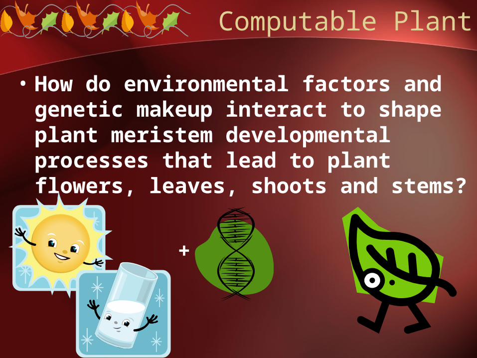
Computable Plant

• How do environmental factors and genetic makeup interact to shape plant meristem developmental processes that lead to plant flowers, leaves, shoots and stems?

+ =

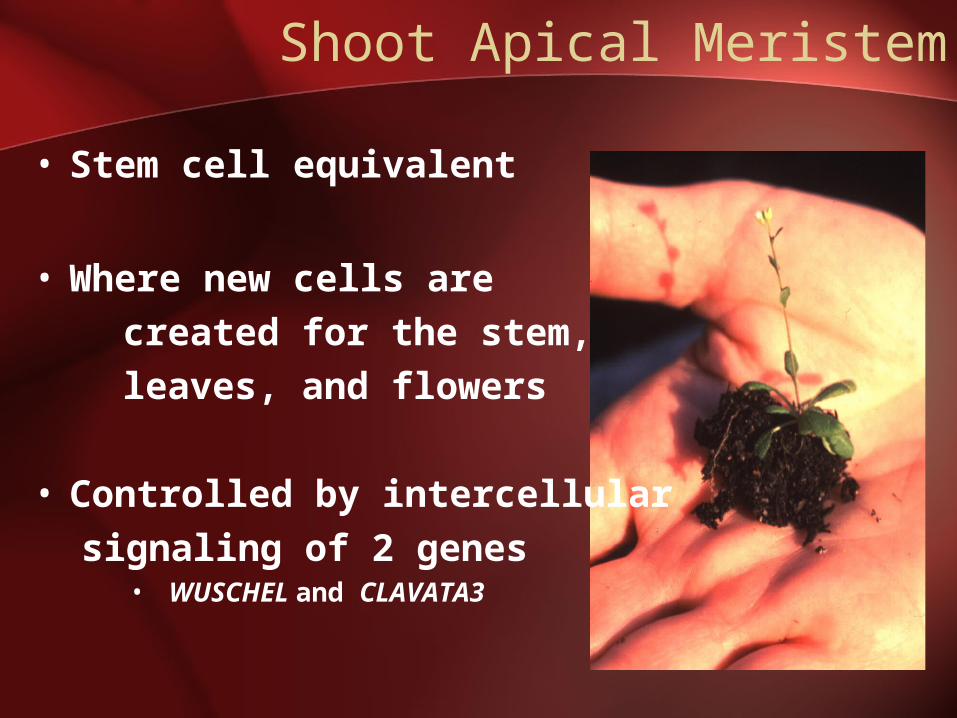
Shoot Apical Meristem

• Stem cell equivalent

• Where new cells are created for the stem, leaves, and flowers

• Controlled by intercellularsignaling of 2 genes

• WUSCHEL and CLAVATA3

WUSCHEL expression

Side View Birds Eye View

Strategy Background

• In paper, model is discrete on extracted template

• Average WUS intensity for individual cells is obtained using confocal microscopy

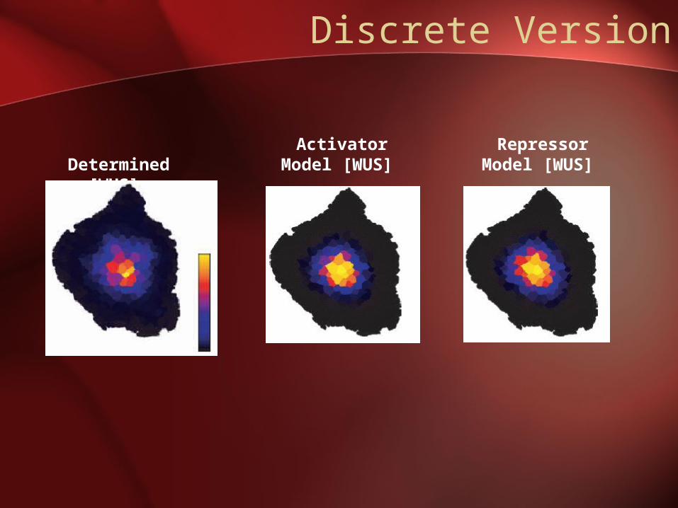
Discrete Version

Determined [WUS]

Activator Model [WUS]

Repressor Model [WUS]

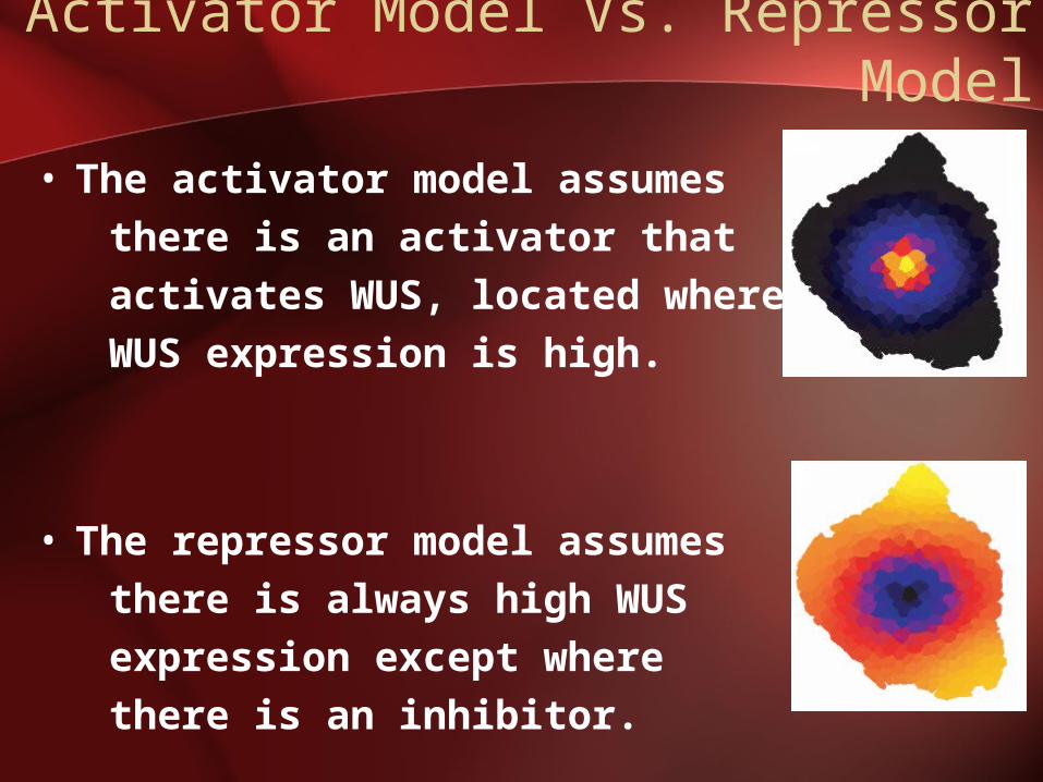
Activator Model Vs. Repressor Model

• The activator model assumes there is an activator that activates WUS, located where WUS expression is high.

• The repressor model assumes there is always high WUS expression except where there is an inhibitor.

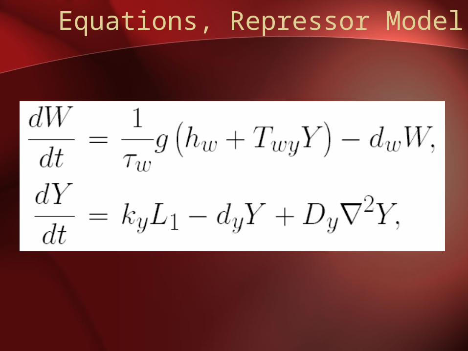
Equations, Repressor Model

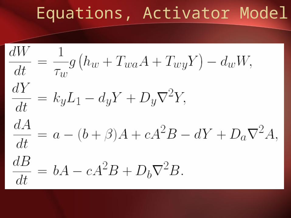
Equations, Activator Model

Goal & Rationale

• Goal:– To extend the models of the gene

expression to a continuous model to see if model still holds

• Rationale:– The models of this project were

created as a way to describe and test several hypotheses

– Further testing the models and extending their applicability simply furthers their research

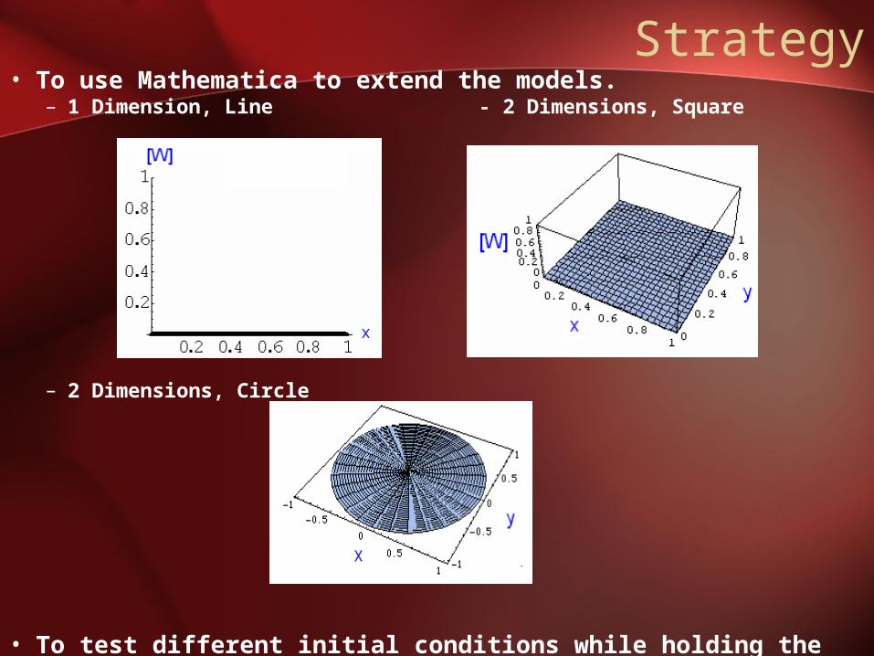
Strategy• To use Mathematica to extend the models.

– 1 Dimension, Line - 2 Dimensions, Square

– 2 Dimensions, Circle

• To test different initial conditions while holding the boundary conditions to 0, as set in the original paper.

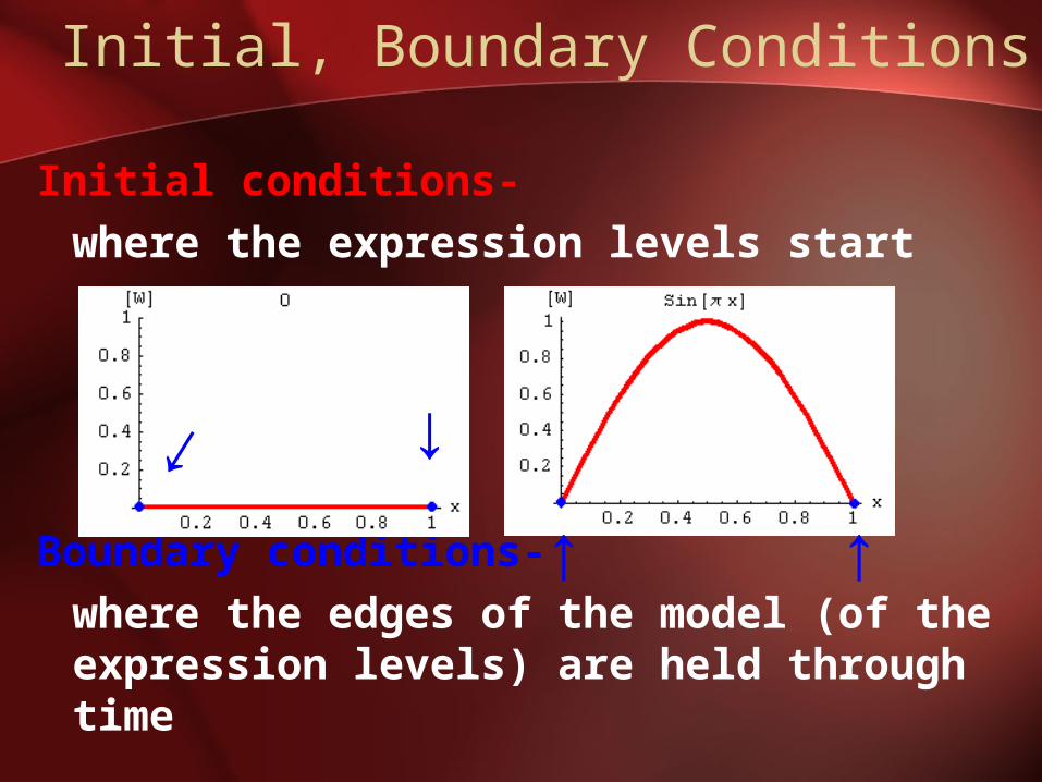
Initial, Boundary Conditions

Initial conditions-where the expression levels start

Boundary conditions-where the edges of the model (of the expression levels) are held through time

↑ ↑

↓↓

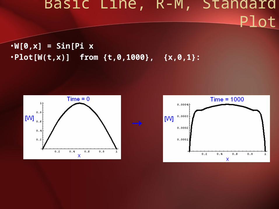
Basic Line, R-M, Standard Plot

•W[0,x] = Sin[Pi x]•Plot[W(t,x)] from {t,0,1000}, {x,0,1}:

•Video:

→

Basic Line, R-M, Standard Plot•W[0,x] = Sin[Pi x](1+Sin[5 Pi x]) •Plot[W(t,x)] from {t,0,1000}, {x,0,1}:

•Video:

→

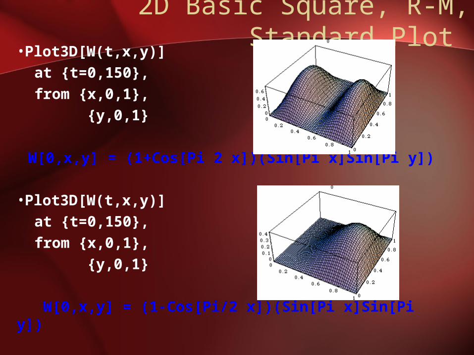
2D Basic Square, R-M, Standard Plot

• Plot3D[W(t,x,y)] at {t=0}, from {x,0,1},

{y,0,1} W[0,x,y] = (1+Cos[Pi 2 x])(Sin[Pi x]Sin[Pi

y])

• Plot3D[W(t,x,y)] at {t=150}, from {x,0,1},

{y,0,1}

2D Basic Square, R-M, Standard Plot

•Plot3D[W(t,x,y)] at {t=0,150}, from {x,0,1},

{y,0,1}

W[0,x,y] = (1+Cos[Pi 2 x])(Sin[Pi x]Sin[Pi y])

•Plot3D[W(t,x,y)] at {t=0,150}, from {x,0,1},

{y,0,1}

W[0,x,y] = (1-Cos[Pi/2 x])(Sin[Pi x]Sin[Pi y])

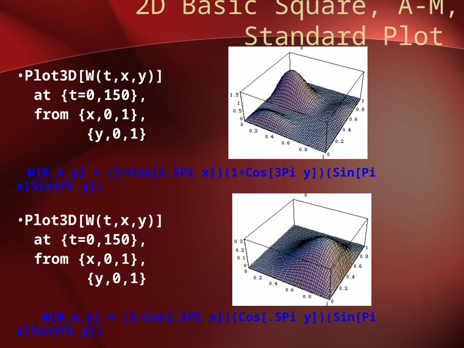
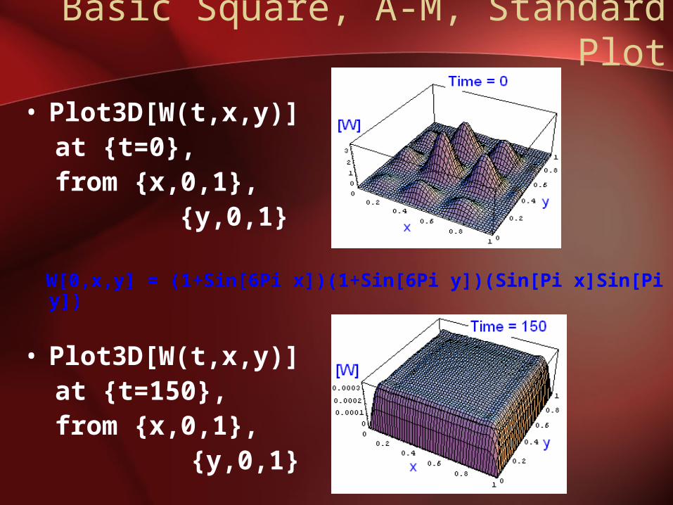
2D Basic Square, A-M, Standard Plot

•Plot3D[W(t,x,y)] at {t=0,150}, from {x,0,1},

{y,0,1}

W[0,x,y] = (1+Cos[1.5Pi x])(1+Cos[3Pi y])(Sin[Pi x]Sin[Pi y])

•Plot3D[W(t,x,y)] at {t=0,150}, from {x,0,1},

{y,0,1}

W[0,x,y] = (1-Cos[.5Pi x])(Cos[.5Pi y])(Sin[Pi x]Sin[Pi y])

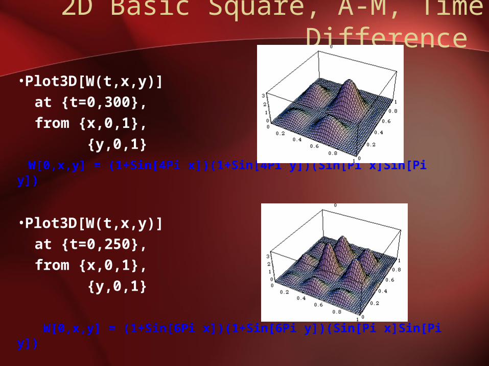
2D Basic Square, A-M, Time Difference

•Plot3D[W(t,x,y)] at {t=0,300}, from {x,0,1},

{y,0,1} W[0,x,y] = (1+Sin[4Pi x])(1+Sin[4Pi y])(Sin[Pi x]Sin[Pi y])

•Plot3D[W(t,x,y)] at {t=0,250}, from {x,0,1},

{y,0,1}

W[0,x,y] = (1+Sin[6Pi x])(1+Sin[6Pi y])(Sin[Pi x]Sin[Pi y])

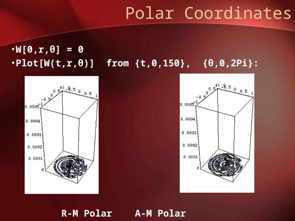
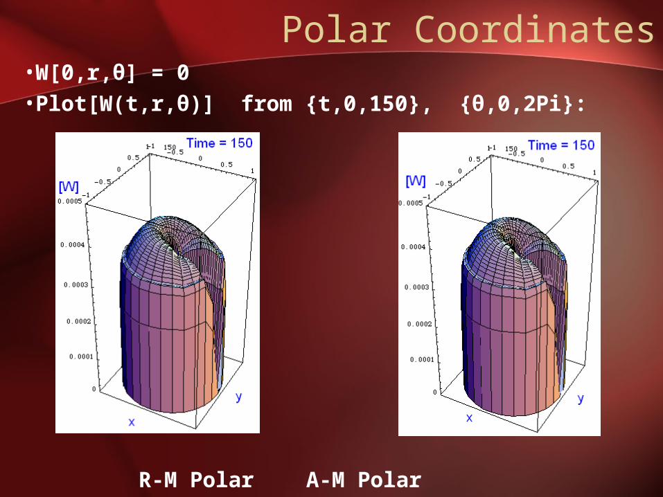
Polar Coordinates

•W[0,r,θ] = 0•Plot[W(t,r,θ)] from {t,0,150}, {θ,0,2Pi}:

R-M Polar A-M Polar

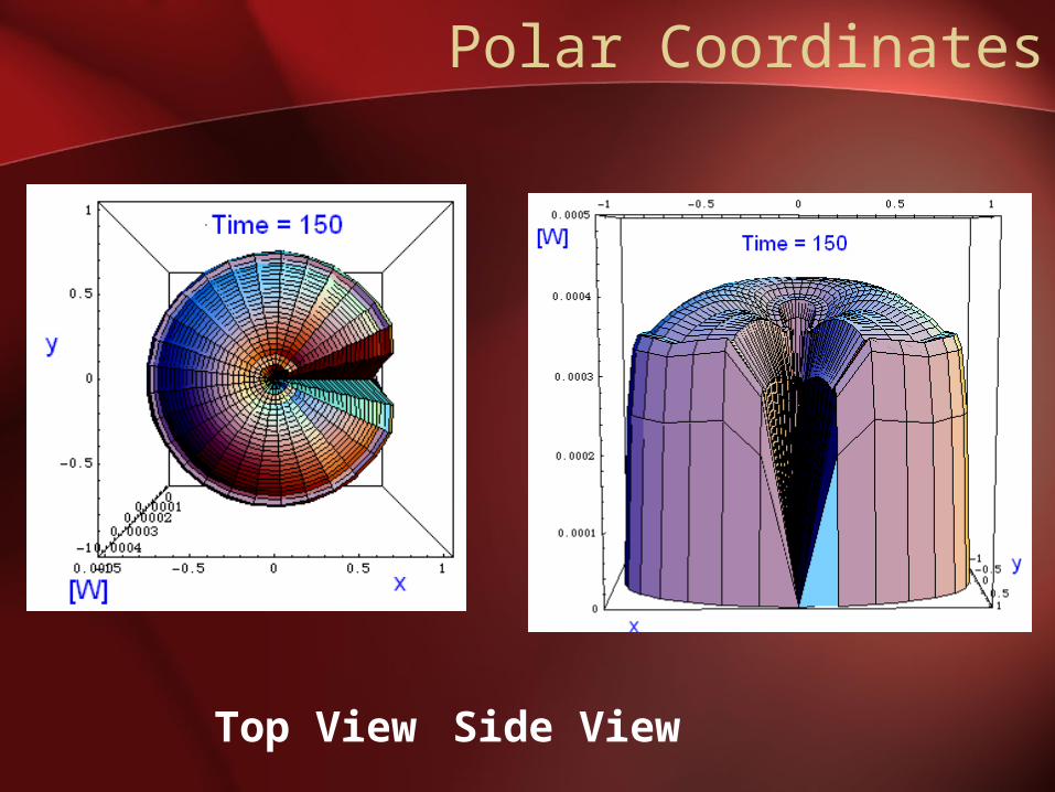
Polar Coordinates

Top View Side View

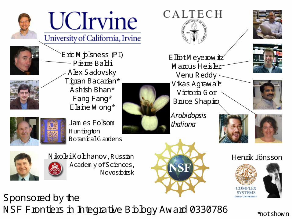
Eric Mjolsness (PI)Pierre Baldi

Alex SadovskyTigran Bacarian*

Ashish Bhan*Fang Fang*

Elaine Wong*

Elliot MeyerowitzMarcus Heisler

Venu ReddyVikas Agrawal*

Victoria GorBruce Shapiro

James FolsomHuntington Botanical Gardens

Nikolai Kolchanov, RussianAcademy of Sciences,

Novosibirsk

Henrik Jönsson

Arabidopsis thaliana

*not shown

Sponsored by theNSF Frontiers in Integrative Biology Award 0330786

References, Acknowledgements

• (2005) Jönsson H, Heisler M, Reddy GV, Agrawal V, Gor V, Shapiro BE, Mjolsness E, and Meyerowitz E.M., Modeling the organization of the WUSCHEL expression domain in the shoot apical meristem. Bioinformatics 21(S1): i232-i240.

• Bruce Shapiro, Ph.D• Computable Plant• SoCalBSI

Basic Line, R-M, Standard Plot

•W[0,x] = Sin[Pi x•Plot[W(t,x)] from {t,0,1000}, {x,0,1}:

→

Basic Line, R-M, Standard Plot•W[0,x] = Sin[Pi x](1+Sin[5 Pi x]) •Plot[W(t,x)] from {t,0,1000}, {x,0,1}:

→

2D Basic Square, R-M, Standard Plot

• Plot3D[W(t,x,y)] at {t=0}, from {x,0,1},

{y,0,1} W[0,x,y] = (1+Cos[Pi 2 x])(Sin[Pi x]Sin[Pi

y])

• Plot3D[W(t,x,y)] at {t=150}, from {x,0,1},

{y,0,1}

Basic Square, A-M, Standard Plot

• Plot3D[W(t,x,y)] at {t=0}, from {x,0,1},

{y,0,1}

W[0,x,y] = (1+Sin[6Pi x])(1+Sin[6Pi y])(Sin[Pi x]Sin[Pi y])

• Plot3D[W(t,x,y)] at {t=150}, from {x,0,1},

{y,0,1}

Polar Coordinates•W[0,r,θ] = 0•Plot[W(t,r,θ)] from {t,0,150}, {θ,0,2Pi}:

R-M Polar A-M Polar

Polar Coordinates

Top View Side View

Eric Mjolsness (PI)Pierre Baldi

Alex SadovskyTigran Bacarian*

Ashish Bhan*Fang Fang*

Elaine Wong*

Elliot MeyerowitzMarcus Heisler

Venu ReddyVikas Agrawal*

Victoria GorBruce Shapiro

James FolsomHuntington Botanical Gardens

Nikolai Kolchanov, RussianAcademy of Sciences,

Novosibirsk

Henrik Jönsson

Arabidopsis thaliana

*not shown

Sponsored by theNSF Frontiers in Integrative Biology Award 0330786

References, Acknowledgements

• (2005) Jönsson H, Heisler M, Reddy GV, Agrawal V, Gor V, Shapiro BE, Mjolsness E, and Meyerowitz E.M., Modeling the organization of the WUSCHEL expression domain in the shoot apical meristem. Bioinformatics 21(S1): i232-i240.

• Bruce Shapiro, Ph.D• Computable Plant• SoCalBSI