Inverse Rendering from a Single Image

Samuel BoivinDynamic Graphics Project, University of Toronto, Canada

Andre GagalowiczMirages Project, INRIA-Rocquencourt, France

AbstractIn this paper, we present a new method to recover an ap-proximation of the bidirectional reflectance distribution func-tion (BRDF) of the surfaces present in a real or syntheticscene. This is done from a single photograph and a 3D ge-ometric model of the scene. The result is a full model ofthe reflectance properties of all surfaces, which can be ren-dered under novel illumination conditions with, for exam-ple, viewpoint modification and the addition of new syn-thetic objects. Our technique produces a reflectance modelusing a small number of parameters. These parametersnevertheless approximate the BRDF and allow the recov-ery of the photometric properties of diffuse, specular, iso-tropic or anisotropic textured objects. The input data area geometric model of the scene including the light sourcepositions and the camera properties, and a single capturedimage. We present several synthetic images that are com-pared to the original ones, and some possible applicationsin augmented reality such as novel lighting conditions andaddition of synthetic objects.

1. Introduction and Motivations

Research in Computer Graphics has been more and moredeveloped over the past few years. This domain has giventhe opportunity to produce photorealistic images using phys-ical or empirical techniques. Even if the resulting imageswere often spectacular, full realism is underachieved whencomparing the computer-generated images with real im-ages captured with a camera. A new field called Image-Based Rendering enhances the quality of image synthe-sis, by directly using the real images to create syntheticones. A subfield known as Inverse Rendering aims to es-timate object reflectances (BRDF) inside a real scene. Us-ing this photometric reconstruction, it is possible to cre-ate new synthetic images under novel illumination condi-tions. Moreover, almost all the techniques in inverse ren-dering use a 3D geometrical model and in some cases thepositions and the intensities of the light sources. Conse-quently many augmented reality applications become ap-pliable. We can add or remove some objects, and thencompute the new interactions between the assembled ob-jects of the scenes. Many authors have contributed to theresolution of the inverse rendering problem [14, 17, 25,24, 26, 18, 19, 27, 6, 32, 15, 16, 23, 22, 11, 10, 21]. Theseworks can be divided into several different categories, de-pending on the complexity of the scene: one isolated ob-ject or a full 3D scene, and the complexity of the illumina-tion: local or global. A lot of work has been accomplished

in the determination of the BRDF for an isolated objectunder specific illumination conditions [14, 17, 25, 24, 26,18, 19], or under general unknown illumination conditions[20]. Some of these techniques are able to produce theexact BRDF from a set images and they generally use atailored approach to achieve this goal. Moreover, the em-phasis of these past works are on the elimination of thecostly measures incurred by the use of a gonioreflectome-ter, rather the creation of new synthetic images. Recently,several other methods have been proposed to extend thephotometric reconstruction to augmented reality applica-tions such as viewpoint moving and illumination changesfor example [6, 32, 15, 16]. These contributions generallyuse a sparse set of photographs to estimate the full BRDFof materials inside a real scene [6, 32, 15, 16]. This oftengenerates additional work for the user, especially if severalimages have to be taken under specific viewpoints [32].Fournier et al. [11] proposed another approach that esti-mates only diffuse reflectances using a single image. Weextend this work by introducing a new hierarchical systemto estimate the full BRDF of objects from a single image,following our previous works in the inverse rendering field[21, 3, 1, 4]. This paper is a description of this work andit includes a new experimental validation on a syntheticscene comparing real and recovered parameters for differ-ent BRDF.

2. Previous Work

All the techniques and ideas in this paper have been madepossible by works about photorealistic rendering includingglobal illumination and ray tracing, image-based model-ing and BRDF modeling. However, this paper falls mainlywithin the description of inverse rendering, image-basedrendering and reflectance recovery. We limit here the over-view of the previous methods to the most relevant algo-rithms to our technique. Therefore, the background de-scribed here includes only techniques which take into ac-count a full 3D scene and use global illumination. A com-plete overview of all the existing algorithms is available in[4, 2].

2.1. Reflectance Recovery from Several Images

Debevec [6] used global illumination for augmented real-ity applications. To insert new objects inside a real im-age, he needed to take into account interreflections andcomputed the reflectances of the surfaces in the part ofthe scene influenced by this insertion. He created a geo-

metrical 3D model of this part of the scene, called the lo-cal scene, and manually calculated the reflectance param-eters of all the modeled objects. Each of the non-diffuseBRDF parameters are changed by the user iteratively untilthe rerendered image becomes close enough to the originalone. The perfect diffuse parameters are set by an automaticprocedure.

Yu et al. [32] proposed a complete solution for the re-covery of surface BRDF from a sparse set of images cap-tured with a camera;

���of the

�����images were taken

specifically to get specular highlights on surfaces. Theybuilt � � radiance maps for the estimation of the reflectanceparameters and the computation of the radiance-to-pixelintensity conversion function (camera transfer function) [7].Using an image-based modeling software such as Facade[8], a 3D geometrical model of the scene was built from theset of images. All the data were then utilized to recover theBRDF of the modeled surfaces. Their method minimizedthe error in the parameters of the Ward’s anisotropic BRDFmodel [29] to estimate the best possible BRDF for eachobject. This work was applied to the insertion of new ob-jects in the scene, to the modification of the illuminationconditions and to the rendering of a new scene under novelviewpoints. However, this method only works if at leastone specular highlight is visible on an object. Otherwisethis object is simulated as perfectly diffuse.

Loscos et al. [15] proposed a method based on an orig-inal idea from Fournier et al. [11]. Their algorithm recov-ered the diffuse reflectances of the surfaces inside a set ofphotographs of a scene, taking into account the textures ofthe objects; each surface has to be unshadowed in at leastone image of the set. They applied their technique to theinsertion/removal of objects and to the modification of thelighting conditions of the original scene. More recently,Loscos et al. [16] extended this technique by removingthe constraint of the unshadowed surfaces. To improve theresults, they transformed their reflectance recovery algo-rithm into an iterative process. However, the method re-mained limited to perfectly diffuse surfaces; the mirrorsare considered to be diffuse textured objects for example.

2.2. Reflectance Recovery from a Single Image

A pioneering work in this domain was completed by Fournieret al. [11] in 1993. He proposed to rerender an original im-age using a 3D representation of the scene, including thepositions of the light source and the camera parameters anda single image of this scene. All the surfaces were consid-ered to be perfectly diffuse, and they used their reprojec-tion onto the real image to estimate their reflectances. Aradiosity-based algorithm then computed an image apply-ing these reflectances to a progressive radiosity technique[5] to obtain a new synthetic image.

An extension of the previous method was developedby Drettakis et al. [10]. They proposed an interactive ver-sion of the initial paper and added a vision algorithm forthe camera calibration and the automatic positioning of the3D geometrical model. They described a slightly differenttechnique for the estimation of the reflectances of the sur-faces and they used a hierarchical radiosity algorithm [13]to compute a new synthetic image similar to the real one.

An approach similar to that of Fournier et al. was cho-

sen by Gagalowicz [21]. It included a feedback that com-pares the real image to the synthetic one. He described atechnique to generate a new synthetic image from a singleimage using an iterative method that minimizes the errorbetween the real image and the synthetic one. Note, how-ever, that the 3D geometrical model obtained in the processwas built from two stereo images. This technique is lim-ited to a pure lambertian approximation of the surface re-flectances. An extension of this work has been realized byBoivin et al. [4], who introduced a new technique takinginto account complex BRDFs of objects inside a real scene.They proposed a hierarchical and iterative method whichminimizes the error between the real and the synthetic im-age to estimate various types of BRDF, such as anisotropicsurfaces. They applied their work to augmented reality ap-plications.

3. Data and Work Base

3.1. Two fundamental data

The method that we propose here requires two data. Firstof all, we need a full three-dimensional geometrical modelof the scene including the intensities and the positions ofthe light sources. The construction of the 3D model can beachieved by many different ways including manual ones.We used Maya (Alias �Wavefront) to manually position the3D geometrical models of objects in the original imageand to approximately build the light sources. All the cam-era parameters have been recovered using the Dementhonand Davis [9] technique combined with a downhill simplexminimization method [12]. However, many other tech-niques can be used to obtain the camera parameters and the3D geometrical model [8]. Moreover, in our algorithm, allthese reconstructed objects must be grouped by the type ofreflectance. This means that the user must declare inside agroup all the objects which are supposed to have the sameBRDF (for example perfectly diffuse or isotropic). Thisis a very important heuristic, because the inverse render-ing algorithm will now be able to compute or attribute re-flectances to objects which are not directly seen in the orig-inal image. This structuring of data also allows for someaugmented reality applications, such as viewpoint modi-fication and object insertion for example. This groupingoperation is a very fast manual operation performed dur-ing of after the modeling step. Finally, the second data thatwe need is one single image of the real scene captured us-ing any camera 1, without any constraint on the position ofthe observer.

3.2. Accuracy of the geometrical model

The precision required by the inverse algorithm for the po-sitioning of the geometrical model tolerates several pixelsof difference between the projection of the model and thereal objects in the image. The acceptable number of mis-classified pixels depends on the size of the projected objectin the original image. For example, if the projection of allobjects belonging to the same group has a total number often visible pixels , then the inverse algorithm will computethe wrong BRDF when at least about three or four of the

1We used a 3xCCD Sony camera, DCR-VX1000E.

ten pixels do not belong to the currently analyzed objects.We use very classical filtering methods, such as edge de-tectors, edge removal filters and a planar approximation, toreduce inconsistencies with the geometrical model by min-imizing the number of pixels assigned to a wrong object.

4. Our inverse rendering algorithm

The inverse rendering algorithm can be described usingtwo concepts: an iterative one and a hierarchical one (seeFigure 1). When the algorithm starts, it considers all theobjects inside the scene as perfectly diffuse. The BRDFsof all the objects are initialized to the average of the radi-ances computed from the pixel intensities 2 covered by theprojection of the group in the original image.

4.1. Overview

Surface assumed to

be perfectly specular

( s =1.0, d=0.0)r r

Surface assumed to

be perfectly diffuse

Surface assumed to be

non-perfectly specular

( r rs <1.0, d=0.0)Non-perfectly specular sur face

Iterative correction of sr

Surface assumed to be

isotropic (rough)

( r r a

r rs <=1.0, d<1.0, )

s + d<=1.0

Minimization on s, ar rd ,

Surface assumed to be

anisotropic (rough)

( r r

a a r rs <=1.0, d<1.0,

x, y, x, s + d<=1.0)

Minimization on x, ya a

Surface assumed to be diffuse

and non-perfectly specular

( r r

r rs <1.0, d<1.0)

s + d<=1.0

Surface assumed to be

textured

( r rd (x,y)<=1.0, s=0.0)

Iterative correction of d(x,y)r

Rendering

Software Phoenix

Diffuse surface

Iterative correction of drComputation of error

(real image - synthetic image)

>threshold <threshold

e

e e

Surface confirmed

as perfectly specular

Surface confirmed as diffuse

and non-perfectly specular

Surface confirmed isotropic

Surface confirmed as anisotropic

Final Synthetic Image

Computation of the anisotropic

direction x (brushed direction)

Storage of the computed d , sr r

Surface confirmed

as perfectly diffuseafter 4 iterations

synth

etic

image

synt

hetic

image

synthetic

image

synthetic image

synthetic image

synth

etic

image

synth

etic

ima

ge

Surface confirmed as

non-perfectly specular

on dr

on sr

Original Real Image

Extraction of the surfaces

Computation of error

(real image - synthetic image)

>threshold <threshold

e

e e

Computation of error

(real image - synthetic image)

>threshold <threshold

e

e eafter 4 iterations

Computation of error

(real image - synthetic image)

>threshold <threshold

e

e e

Computation of error

(real image - synthetic image)

>threshold <threshold

e

e e

Computation of error

(real image - synthetic image)

>threshold <threshold

e

e e

Computation of error

(real image - synthetic image)

threshold threshold

e

e< e>

Iterative correction of dr

Iterative correction of sr

Figure 1: General iterative and hierarchical algorithm for reflectance recovery.Each surface of the scene is analyzed separately, depending on the assumption aboutits reflectance (perfectly diffuse, perfectly specular, etc.). If the assumption is false(the error between the real and the synthetic image is big), then the surface re-flectance is assumed to be more complex (hierarchical principle). If the assumptionis correct then the surface reflectance is modified accordingly in order to minimizethe error between the two images (iterative principle). During each global rerender-ing iteration, the reflectances of all surfaces are then continuously updated, to takeinto account the incident energy coming from any surface for which the BRDF haschanged (a diffuse surface modified to be perfectly specular for example).

Following this diffuse assumption, our algorithm computea new synthetic image using photo-realistic rendering tech-niques 3. Our inverse method attempts to minimize the er-ror between the real and the synthetic image in order to

2These radiances have been obtained using the inverse of the cameratransfer function that was simulated as a � correction function with a �value of 2.2 according to Tumblin et al. [28]. However a more powerfulalgorithm could be applied if we had more than one photograph of ourscene [7].

3We use our own rendering software called Phoenix [2] to computethe new images, but any global illumination software such as Radiance[30] can be used as well

obtain the best possible approximation for the BRDF. Theiterative step seeks the best parameters following a givenassumption about the BRDF. The hierarchical step changesthe hypothesis regarding the BRDF if the iterative step failsto obtain a small error between the real and the syntheticimage.Each time a new image has been generated, an image dif-ference is then computed to determine which object BRDFmust be changed. If the perfectly diffuse assumption pro-duces a big error between the two images for a given group,then the inverse rendering algorithm chooses another hy-pothesis regarding the reflectance of this group. It triesa more complex BRDF model (a perfectly specular onehere). Again, Phoenix generates a new synthetic imageusing the new hypothesis, and the inverse algorithm com-putes a new error image to determine which object BRDFmust be modified. As we can see, the inverse algorithmuses more and more complex hypotheses (hierarchical prin-ciple) to obtain the correct BRDF and the correspondingparameters. Several hypotheses are successively appliedand the algorithm stops when the error between the realand the synthetic image is smaller than a global user-definedthreshold. The determination of the thresholds is not criti-cal to our method and it can be found in [2, 4].

4.2. Computing the Ward’s BRDF parametersAll the BRDF parameters that are estimated here, comefrom the Ward’s BRDF model[29]. We chose the sameBRDF model as Yu et al. [32] because of its small numberof parameters and its ability to simulate anisotropic sur-faces. This model only requires the knowledge of five pa-rameters for a complex BRDF: ��� the diffuse reflectance,��� the specular reflectance, �� the anisotropy direction (call-ed the brushed direction) and the anisotropic roughness pa-rameters � and �� . Furthermore, this model avoids thecostly computation of the Fresnel term which has been re-placed by a normalization factor. A detailed description ofthis BRDF model can be found in [29].

4.2.1. Perfectly diffuse surfacesThe perfectly diffuse case is very simple because only oneparameter ( ��� ) has to be computed. During the first iter-ation, all objects are assumed to be perfectly diffuse. Ev-ery reflectance for each group is initialized to the averageof the radiances covered by the projection of the group inthe original image. Phoenix generates a new synthetic im-age using these reflectance. A new error is computed asthe ratio between the average of the radiances covered bythe projection of the groups in the original image, and theaverage of the radiances covered by the projection of thegroups in the synthetic image (see equation 1). This errorbalances the original diffuse reflectance, and after severaliterations an optimum value of ��� is found 4.

� �������� �� ��� �

��������� � � �"!�� ��� � �#� �$! (1)

where:���� � and�� � � are respectively the average of the radiances and the pixels covered

by the projection of object % in the original image.� ��� � and��#� � are respectively the average of the radiances and the pixels covered

by the projection of object % in the synthetic image.��� ! is the camera transfer function.

4it is shown in [2] that only 4 iterations are sufficient to converge toan optimum value of &"'

Since the average radiance��% of object � is proportional

to the diffuse reflectance ��� % , the iterative correction of the��� % can be written for each rerendering iteration � as:����� � � ������� � � � � (2)

����� � � ������� � �� ����� ��� � � �� !�� � � ������ � !� ��

��� ��� � � �� !�� � �� ��� �����(3)

and � � � �� ! � �"! if� ��$# �&%('*) !�� � �%

elsewhere:� � and

� �� are respectively the total error between the original and the synthetic im-age for group + and object % ., � is the number of objects for group + .� � is the median of the errors (selects the middle value of the sorted samples).)

is the authorized dispersion criteria.� � is the number of pixels covered by the projection of object % .The function � � ! eliminates problems generated by smaller objects for which theerror is very important, because they are more sensitive to the image noise (theirprojection in the image covers a small amount of pixels). An example of iterativecorrection of ��� (and ��- ) is provided by Figure 2 on a simple real interior scene,containing both diffuse and specular objects.

After several iterations, a new error image is still computedas the difference between the real and the latest syntheticimage. If this error remains bigger than a user-definedthreshold for a given group, then the algorithm now de-cides that all these objects are perfectly specular.

4.2.2. Perfectly and non-perfectly specular surfaces

In the case of perfectly specular surfaces, it is extremelyeasy to compute the reflectance parameters, because � � hasa null value and ��� is constant ( ���/. �

). A new syntheticimage can be immediately generated taking into accountthe new BRDF. But, if the new error for objects assumedas perfectly specular remains large, the algorithm tries toenhance the ��� parameter. This new type of BRDF corre-sponds to the non-perfectly specular case. This specularparameter is modified according to equation 3 applied to��� instead of ��� . The images of Figure 2 have been gener-ated using this technique and clearly shows a significantdecrease in the error during the inverse rendering itera-tions.If the resulting synthetic image still differs from the origi-nal one in terms of error (image difference by group of ob-jects), then the diffuse and specular hypothesis is applied.

70

0

27

54

Sum

of th

e 3

R,G

,B e

rro

rs

( in

pix

el i

nte

nsi

ties

)

Figure 2: Simulation of hierarchical inverse rendering, where the top row fromleft to right consists of the real image captured with a camera, the synthetic imagewith a pure diffuse assumption (first iteration), the synthetic image with perfect dif-fuse and perfect specular assumptions (fifth iteration) and the synthetic image withpure diffuse and non-perfect specular surfaces (seventh iteration). On the bottomrow, we can see the error images corresponding to the difference between the realand the synthetic image.

4.2.3. Both diffuse and specular surfaces

In the Ward’s BRDF model [29], we now consider the casewhere ��� and ��� have a non-null value. All the surfaces areassumed perfectly smoothed which means that there is noroughness factor to compute.These two parameters can be analytically estimated by min-imizing the error between the real image and the syntheticimage as a function of ��� and ��� :

� � -10 �325476 ����8�9 !;: � �=<;9� � � � � ��� � � � ' ��- � � - 6 � ����8�9 ! !;:where:,?>1@ , the number of pixels covered by the group projection.� -10 �3254 , ����8�9 the pixel intensities converted to radiances respectively for the syn-

thetic and the original images.

This minimization has an analytical solution for each wave-length ACBEDFB � :GFH �H -JI �LKMMN � �=<;9�O �QP O ��8�9QR�

�=<;9�O - P O ��8�9QRS3TTU KMMN

��=<;9�O :� �

�=<;9�O � O -��=<;9�O � O - �

�=<;9VO :-S3TTU���

In practice, such surfaces in real cases are very rare but notimpossible. For example, the top face of the desk in Figure9 presents some photometric properties very close to thisapproximation.

4.2.4. Isotropic surfaces

In order to solve the case of isotropic surfaces, we mustnow find three parameters: the diffuse reflectance � � , thespecular reflectance ��� and the roughness parameter � [29].In most cases, a direct minimization algorithm can be usedto find these parameters. However, we have shown in [4]that it is not always easy to minimize such a function.Therefore, it could be useful to separate the case � �W. �from the other cases. We then minimize these two casesseparately using a downhill simplex method [12] and wechoose the parameters which produce the smallest error.

Figure 3 shows the result of these minimizations: thealuminium surface (in the center of image) has been sim-ulated as isotropic, and an optimum value of � �X. �(Y � �and ���L. �(Y Z?[

has been found. However the error im-age shows that a better approximation might be possiblefor this particular surface. The error remains important inthe region bordering the specular reflection area of the twobooks on this surface. Therefore a more complex BRDFis needed and the algorithms now attempts to simulate thesurface as an anisotropic one.

70

27

54

0

Sum

of th

e 3

R,G

,B e

rro

rs

( in

pix

el i

nte

nsi

ties

)

Error image for the glossy surface

simulated as an isotropic one

Figure 3: Approximation of the aluminium surface (anisotropic) of the real im-age (left) by an isotropic surface in the synthetic image (center). The error betweenthese two images for the aluminium surface is visible in the right image. We notethat the error is still important in the area of the specular reflection of the books.The red pixels correspond to a high error but they are not significant because theyare coming from an approximate positioning of the 3D geometrical model on theimage, especially on the edges of the objects.

4.2.5. Anisotropic surfaces

In the case of isotropic surfaces, we saw that we had threeparameters to compute ( ��� , ��� and � ). For the anisotropiccase, we must now compute the anisotropy direction ( �� )andtwo other roughness parameters ( � , �� ) replacing the pre-vious � in the isotropic case. It has been shown in [4] thata direct minimization algorithm to estimate these param-eters produces results of poor quality even if the methodconverges. Therefore we propose a direct estimation ofthe anisotropy direction from the original image.If we could zoom in, we could see that an anisotropic sur-face has small wave-like features (roughness) on the sur-faces characterized by a common direction. This directioncalled the brushed direction is the anisotropy direction thatwe are looking for. These waves are clearly visible on theleft image of Figure 4 computed for an anisotropic surface.However, they are not directly visible from the original im-age: the left image of Figure 4 is displayed as a 3D surfaceand it is produced from several processing steps that aredescribed below.

In a first step, we consider the anisotropic surface asa perfect mirror and compute a synthetic image. Next, weestimate the difference between the real image and the syn-thetic one to visualize the part of the anisotropic mirrorwhere the specular reflection is “extended”. This area cor-responds to an attenuation of the specular reflection, andthis effect is always very important in the direction perpen-dicular to the brushed direction (or anisotropy direction).

24

68Y Coord

1012

1416

10

20

30

40

50 X Coord

60

70

0

100

200

300

Sum of the R,G,B errors(in pixel intensities)

−80 −60 −40 −20 0 20 40 60 80

25

30

35

40

45

θ (degrees)

stan

dard

dev

iatio

n

Figure 4: The selected object used here to recover the anisotropy direction is theviolet book of the lower left real image of figure 9. The 3D surface (left image)shows the error image for the difference between the perfect specular reflection areaof this selected object, and its corresponding area in the real image. The 2D curve(right) shows the average of the standard error deviations computed from the errorimage along the sampled anisotropy directions (see also figure 5).

In a second step, we compute an index buffer for thismirror of all the surfaces visible through it. We then lookfor a reference surface that has the biggest reflection areaon the anisotropic surface, while being as close as possi-ble to it. This surface is then selected in such a mannerthat the ratio Area(reflected surface)� ����� � ! is maximized (withd(S,P), the euclidean distance between the center of grav-ity of the selected surface and the center of gravity of theanisotropic mirror). The motivation of this choice residesin the fact that surfaces very far from the anisotropic objectexhibit a reflection pattern that is too small or too noisy tobe usable for the recovery of the brushed direction. In athird step, the anisotropy direction is sampled creating ��vectors around the normal to the anisotropic surface. Eachof these sampled directions determine a direction to tra-verse the error image and compute the average of the stan-dard error deviations computed in the error image. Finally,the algorithm selects the direction for which this averagevalue is the smallest one (see Figure 4). Figure 5 summa-rizes the complete procedure.Once the anisotropy direction �� has been recovered, a down-

hill simplex minimization algorithm is used to estimate theroughness parameters � and �� .

Original real image

Index buffer of the surfaces

Extraction of the surface assumed to be anisotropic

N

X7

X6X5X3X2

X1

X0

Anisotropic surface

q =00

o

X4

q =402

o

q =201

o

X8

70

27

54

0Sum

of th

e 3

R,G

,B e

rro

rs

( in

pix

el i

nte

nsi

ties

)

Rendering of the surface assumed to be anisotropic

as a perfectly specular surface, and extraction of

the area from the synthetic image

Computation of the index buffer of the surfaces

reflected on the perfect mirror. Selection of the

surface for which the ratio of its reflected area

on the mirror divided by the distance between

its center of gravity and the center of gravity of

the mirror, is the biggest one.

Extraction of the surface

simulated as a perfect

mirror in the synthetic image

Extraction of the surface

assumed to be anisotropic

in the real imageComputation of the error

image between the perfectly

specu la r a rea and the

corresponding anisotropic area

Sampling of the brushed direction x around

the normal N to the anisotropic surface,

with respect to a rotation angle q

Computation of the standard

deviations on the error image

in the x direction

Selection of the x direction for

which the average of the

standard deviations is the

smallest. This vector x is the

or theanisotropy direction

brushed direction.

Figure 5: Computation method of the anisotropy direction � for a glossy surface.

4.2.6. Textured surfaces

When the anisotropic simulation of a surface still produceslarge errors in the difference image, we proceed to textureextraction.

Extracting the texture from the real image is an easytask that can be realized using the technique proposed by[31] for example. However, we have to extract this tex-ture while taking into account the fact that it already hasreceived the energy from the light sources, and that thepixels covered by its projection in the real image containthis information. Otherwise, if we send the energy of thelight sources to these textures again, they will be over-illuminated. Therefore, we introduce a notion called ra-diosity texture that balances the extracted texture with anintermediate texture in order to minimize the error betweenthe real and the synthetic image. As for the perfectly dif-fuse reflectance case, this intermediate texture is computedby an iterative method.

At the first iteration, the texture used to rerender theimage is the texture directly extracted from the real image.At the second iteration, the texture used to obtain the re-sulting synthetic image is multiplied by the ratio betweenthe newly extracted texture of this synthetic image and thetexture of the real image. This iterative process stops whenthe user-defined threshold for textured surfaces has beenreached. The textures of the poster and the books in thererendered images of Section 4.3.2 have been obtained us-ing this technique. The problem of this method is that itcomputes a texture including the shadows, the specular re-flections and the highlights. As an example, consider amarbled floor on which a sphere is reflected. The texture ofthis floor in the real image then includes the marble charac-teristics, its reflectance properties and the sphere reflectionincluding its own reflectance properties. How then do we

Som

me

des e

rreur

s pou

r R,V

,B(e

n in

tens

ités d

e pi

xels)

3

0

1

2

Figure 6: From left to right: original anisotropic floor, floor simulated as an isotropic object, and the error image between the original and the rerendered images.

extract the marble characteristics and independently of therest of the scene ? This is an extremely hard problem, andY. Sato et al. [26] have stated that no algorithm has yetbeen proposed to solve it using a single image.

4.3. Results and computation times

4.3.1. Comparison of recovered parameters

In this section, we propose to give the values obtained forthe recovered BRDF of a computer-generated scene (seeleft image of Figure 7). We compare them to the origi-nal known values used to render the original image withPhoenix.

Figure 7: Left: the original computer-generated image. Right: the new syntheticimage produced by our inverse rendering technique.

The first level of the hierarchy in the inverse render-ing process computes all the parameters of the surfacesin a straightforward manner. However, the error remainslarge for the floor and the next levels are tested for this ob-ject. The specular assumptions (perfectly, non-perfectly,both diffuse and specular) produced large errors forcingthe algorithm to choose the isotropy hypothesis. Duringthe isotropy case, a global minimum has been found for��� , ��� and � , and the synthetic image is visually very closeto the original as shown by Figure 6. However, as we onlyset

���for the maximum tolerated error to switch from the

isotropy hypothesis to the anisotropy, our method tries tosimulate the floor as an anisotropic object.

Using the method described in Section 4.2.5, our algo-rithm finds all the reflectance parameters for the anisotropicobject. All the recovered values are summarized in Figure8 and the final resulting image is shown in Figure 7.

4.3.2. Rerendered scenes

All the following synthetic images have been generated us-ing Phoenix as the rendering and inverse rendering soft-ware. The first synthetic image at the top right of Figure9 has been generated in 37 minutes using the hierarchi-cal algorithm from the left real photograph. Two specularsurfaces have been recovered and simulated as non-perfectmirrors and 14 rerendering iterations were necessary togenerate the final image.

Surface Var Real Computed

Left wall ��� (0.66, 0.66, 0.66) (0.65916, 0.66075, 0.66037)��- (0.0, 0.0, 0.0) (0.0, 0.0, 0.0)

Right Wall ��� (0.69, 0, 0.95) (0.69002, 0.0, 0.95901)��- (0.0, 0.0, 0.0) (0.0, 0.0, 0.0)

Back Wall ��� (0.65, 0.65, 0.0) (0.64997, 0.65067, � � % ! ��� )��- (0.0, 0.0, 0.0) (0.0, 0.0, 0.0)

Ceil ��� (1.0, 1.0, 1.0) (1.0, 1.0, 1.0)��- (0.0, 0.0, 0.0) (0.0, 0.0, 0.0)

Big Block ��� (0.77, 0.0, 0.0) (0.77002, � � % ! ��� , � � % ! � )��- (0.0, 0.0, 0.0) (0.0, 0.0, 0.0)

Small Block ��� (0.0, 0.76, 0.26) (0.0, 0.75802, 0.25912)��- (0.0, 0.0, 0.0) (0.0, 0.0, 0.0)

Floor ��� (0.1, 0.1, 0.1) (0.10013, 0.10045, 0.09981)��- (0.9, 0.9, 0.9) (0.89909, 0.90102, 0.89903)�

0.0�

2.8�

�� 0.07 0.06999�?0 0.11 0.1101

Figure 8: Comparison between the recovered reflectance parameters and theiroriginal values. Note that Ceil is not directly visible in the original image. Whenthis happens, the algorithm considered this object as a perfect diffuse white object.In practice, if such a case happens, the user should find an object whose photometricproperties are close to Ceil. Ceil will then be declared in the same group as thisobject.

The inverse algorithm required 4 hours and 40 min-utes to produce the image at the bottom right of Figure 9.Roughly 4 hours of this time were necessary to recover theanisotropic BRDF of the aluminium surface. The final ren-dering stage required 32 minutes to render the final image(100 bounced rays have been used for the anisotropic sur-face).

The images of Figure 11 show examples of applica-tions in augmented reality. Some synthetic objects havebeen added such as a small robot and a luxo-like desklamp. It is also possible to modify the reflectances with-out much difficulty. New viewpoints can be generated andnew illumination conditions can be created as well.

5. Conclusion and Future Work

In this paper, we have presented a new technique to deter-mine an approximation of the reflectance properties of thesurfaces of a 3D scene, and we have proposed an experi-mental validation of our method. An incremental and hi-erarchical algorithm iteratively estimates various types ofreflectance parameters, including anisotropic and texturedsurfaces. The method takes as input a single photographof the scene taken under known illumination conditions aswell as a 3D geometric model of the scene. The result is acomplete description of the photometric properties of thescene which may be used to produce a photorealistic syn-thetic image very similar to the real one. We showed thatthe method is robust and gives the opportunity to displaythe original scene from novel viewpoint, with unrestrictedillumination conditions and with the addition, removal and

Figure 9: Example of a pure diffuse approximation of a whole 3D scene. From left to right: the original image captured with a camera, the synthetic image and a syntheticimage generated under a new viewpoint. The perfect diffuse assumption is realistic enough for many surfaces, except the computer monitor and the door. Moreover, evenif the desk is a real anisotropic surface, a pure diffuse approximation produces a realistic enough result for this object. Note that a book on the left bookshelf has not beenmodeled. Due to the filtering step and the principle of the method, this does not disturb the inverse rendering case. However, this remains true only for small objects that donot interact much with the real environment. A “very“ large error in the modeling step would definitely produce wrong results.

modification of objects.Currently , our work has some limitations, especially

regarding textured surfaces. Until now, we are not able todiscriminate the shadows or highlights from an assumedtextured surface. In this regard, it will be interesting to ex-tend our method to these cases, although we think that thisis a very difficult problem, if one remains restricted to asingle image.

Moreover, several other extensions are possible becauseof the hierarchical property of our technique. For instance,we may extend the reflectance recovery algorithm to ob-jects that have more complex photometric properties suchas light beams, small fires and caustics as a few examples.

Acknowledgments

The authors would like to thank Jean-Marc Vezien for pro-viding the 3D geometrical model and the camera calibra-tion for the scenes shown in the results section. We alsoacknowledge Glenn Tsang for his helpful suggestions re-garding the writing of this paper.

References1. Jacques Blanc-Talon and Dan Popescu. Advances in Computation: Therory and Practice, chapter Ad-

vanced Computer Graphics and Vision Collaboration Techniques for Image-Based Rendering (SamuelBoivin and Andre Gagalowicz). Nova Science Books and Journals, New York, NY., 2000.

2. Samuel Boivin. Simulation Photorealiste de Scenes d’Interieur a partir d’Images Reelles. PhD thesis,Specialite Informatique, Ecole Polytechnique, Palaiseau, January 2001.

3. Samuel Boivin and Laroussi Doghman. A new rendering technique for the realistic simulation of naturalscenes. In Proceedings of IMAGECOM’96, pages 302–307, 1996.

4. Samuel Boivin and Andre Gagalowicz. Image-based rendering of diffuse, specular and glossy surfacesfrom a single image. Proceedings of SIGGRAPH 2001, pages 107–116, August 2001. ISBN 1-58113-292-1.

5. Michael F. Cohen, Shenchang Eric Chen, John R. Wallace, and Donald P. Greenberg. A progressive refine-ment approach to fast radiosity image generation. In John Dill, editor, Computer Graphics (SIGGRAPH’88 Proceedings), volume 22, pages 75–84, August 1988.

6. Paul Debevec. Rendering synthetic objects into real scenes: Bridging traditional and image-based graphicswith global illumination and high dynamic range photography. In Michael Cohen, editor, Proceedings ofSIGGRAPH 98, Computer Graphics Proceedings, Annual Conference Series, pages 189–198. AddisonWesley, July 1998.

7. Paul E. Debevec and Jitendra Malik. Recovering high dynamic range radiance maps from photographs. InTurner Whitted, editor, Proceedings of SIGGRAPH 97, Computer Graphics Proceedings, Annual Confer-ence Series, pages 369–378. Addison Wesley, August 1997.

8. Paul Ernest Debevec. Modeling and Rendering Architecture from Photographs. PhD thesis, University ofCalifornia, Berkeley, 1996.

9. D.F DeMenthon and L. Davis. Model-based object pose in 25 lines of code. In Second European Confer-ence on Computer Vision(ECCV), pages 335–343. Springer-Verlag, May 1992.

10. George Drettakis, Luc Robert, and Sylvain Bougnoux. Interactive common illumination for computeraugmented reality. In Julie Dorsey and Philipp Slusallek, editors, Eurographics Rendering Workshop1997, pages 45–56. Springer Wien, June 1997.

11. Alain Fournier, Atjeng S. Gunawan, and Chris Romanzin. Common illumination between real and com-puter generated scenes. In Graphics Interface ’93, pages 254–262. Canadian Information ProcessingSociety, May 1993. Held in Toronto, Ontario, Canada.

12. Press W. H., Teukolsky S.A., Vetterling W.T., and Flannery B.P. Numerical Recipes in C, The Art of Scien-tific Computing, chapter 10.4 Downhill Simplex Method in Multidimensions, pages 305–309. CambridgeUniversity Press, Cambridge, 1992.

13. Pat Hanrahan, David Salzman, and Larry Aupperle. A rapid hierarchical radiosity algorithm. ComputerGraphics (Proceedings of SIGGRAPH 91), 25(4):197–206, July 1991.

14. G. Kay and T. Caelli. Inverting an illumination model from range and intensity maps. CGVIP: ImageUnderstanding, 59:183–201, 1994.

15. C. Loscos, M. C. Frasson, G. Drettakis, B. Walter, X. Grainer, and P. Poulin. Interactive virtual relight-ing and remodeling of real scenes. Available from www.imagis.imag.fr/Publications RT-0230, InstitutNational de Recherche en Informatique en Automatique (INRIA), Grenoble, France, April 1999.

16. Celine Loscos, George Drettakis, and Luc Robert. Interactive virtual relighting of real scenes. IEEETransactions on Visualization and Computer Graphics, 6(3):289–305, 2000.

17. J. Lu and J. Little. Reflectance function estimation and shape recovery from image sequence of rotatingobject. In International Conference on Computer Vision, pages 80–86, June 1995.

18. Stephen R. Marschner and Donald P. Greenberg. Inverse lighting for photography. In Proceedings of theFifth Color Imaging Conference. Society for Imaging Science and Technology, November 1997.

19. Stephen R. Marschner, Stephen H. Westin, Eric P. F. Lafortune, Kenneth E. Torrance, and DonaldP.Greenberg. Image-based brdf measurement including human skin. In Dani Lischinski and Greg WardLarson, editors, Eurographics Rendering Workshop 1999. Eurographics, June 1999.

20. Ravi Ramamoorthi and Pat Hanrahan. A signal-processing framework for inverse rendering. Proceedingsof SIGGRAPH 2001, pages 117–128, August 2001. ISBN 1-58113-292-1.

21. A. Rosenblum. Data Visualization, chapter Modeling Complex indoor scenes using an analysis/synthesisframework (Andre Gagalowicz). Academic Press, 1994.

22. Imari Sato, Yoichi Sato, and Katsushi Ikeuchi. Illumination distribution from brightness in shadows:Adaptive extimation of illumination distribution with unknown reflectance properties in shadow regions.In Proceedings of IEEE ICCC’99, pages 875–882, September 1999.

23. Kosuke Sato and Katsushi Ikeuchi. Determining reflectance properties of an object using range and bright-ness images. IEEE Transactions on Pattern Analysis and Machine Intelligence, 13(11):1139–1153, 1991.

24. Yoichi Sato and Katsushi Ikeuchi. Temporal-color space analysis of reflection. Journal of Optical Societyof America, 11(11):2990–3002, November 1994.

25. Yoichi Sato and Katsushi Ikeuchi. Reflectance analysis for 3d computer graphics model generation.Graphical Models and Image Processing, 58(5):437–451, 1996.

26. Yoichi Sato, Mark D. Wheeler, and Katsushi Ikeuchi. Object shape and reflectance modeling from obser-vation. In Turner Whitted, editor, Computer Graphics, Proceedings of SIGGRAPH 97, pages 379–388.Addison Wesley, August 1997.

27. Siu-Hang Or Tien-Tsin Wong, Pheng-Ann Heng and Wai-Yin Ng. Image-based rendering with control-lable illumination. In Julie Dorsey and Phillip Slusallek, editors, Rendering Techniques ’97 (Proceedingsof the Eighth Eurographics Workshop on Rendering), pages 13–22, New York, NY, 1997. Springer Wien.ISBN 3-211-83001-4.

28. Jack Tumblin and Holly Rushmeier. Tone reproduction for realistic images. IEEE Computer Graphicsand Applications, 13(6):42–48, November 1993.

29. Gregory J. Ward. Measuring and modeling anisotropic reflection. In Edwin E. Catmull, editor, ComputerGraphics (SIGGRAPH ’92 Proceedings), volume 26, pages 265–272. ACM Press, July 1992.

30. Gregory J. Ward. The RADIANCE lighting simulation and rendering system. In Andrew Glassner, editor,Proceedings of SIGGRAPH ’94 (Orlando, Florida, July 24–29, 1994), Computer Graphics Proceedings,Annual Conference Series, pages 459–472. ACM SIGGRAPH, ACM Press, July 1994. ISBN 0-89791-667-0.

31. George Wolberg. Digital Image Warping. IEEE Computer Society Press, Los Alamitos, 1990.32. Y. Yu, P. Debevec, J. Malik, and T. Hawkins. Inverse global illumination : Recovering reflectance mod-

els of real scenes from photographs. In A. Rockwood, editor, Computer Graphics (SIGGRAPH 1999Proceedings), volume 19, pages 215–224. Addison Wesley Longman, August 1999.

BiographySamuel Boivin is currently a post-doctoral researcher in the Dy-namic Graphics Project at the University of Toronto. He receivedan M.S. in Computer Graphics from Compiegne University ofTechnology (U.T.C) in 1995, and a Ph.D. in Computer Sciencefrom Ecole Polytechnique in Palaiseau (France) in January 2001.His current research interests are physical simulation and inverserendering. Among his publications, he recently presented a newimage-based rendering technique at the SIGGRAPH 2001 con-ference, co-authored with Andre Gagalowicz.

Andre Gagalowicz is a research director at INRIA (France). Heis the creator of the first laboratory involved in image analy-sis/synthesis collaboration techniques. He graduated from EcoleSuperieure d’Electricite in 1971, obtained a Ph.D in AutomaticControl from the University of Paris XI (1973), and a state doc-torate in Mathematics from the University of Paris VI (1983).His research interests are in 3D approaches for computer vision,computer graphics, and their cooperation. He has published morethan one hundred publications related to these fields in many jour-nals and conferences, and he contributed in the writing of fivebooks.

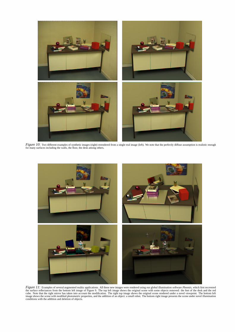
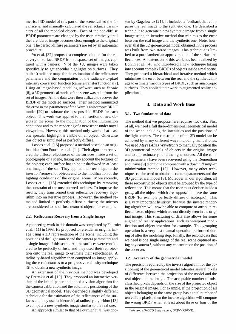
Figure 10: Two different examples of synthetic images (right) rerendered from a single real image (left). We note that the perfectly diffuse assumption is realistic enoughfor many surfaces including the walls, the floor, the desk among others.

Figure 11: Examples of several augmented reality applications. All these new images were rendered using our global illumination software Phoenix, which first recoveredthe surface reflectances from the bottom left image of Figure 9. The top left image shows the original scene with some objects removed: the feet of the desk and the redcube. Note that the right mirror has taken into account the modification. The right top image shows the original scene rendered under a novel viewpoint. The bottom leftimage shows the scene with modified photometric properties, and the addition of an object: a small robot. The bottom right image presents the scene under novel illuminationconditions with the addition and deletion of objects.