
1994 a New ion Scheme for the Inverse Kinematics Tasks of Flexible Robot Arms (2)
I J C T A, 9(7), 2016, pp. 3211-3229© International Science Press
Inverse Kinematics Solution of aFive Joint Robot Using MRAN AlgorithmI.J. Rohit*, I. Jacob Raglend** and M. Dev Anand***
ABSTRACT
One of the significant problem in robot kinematics is to optimising the solution of inverse kinematics which dealswith obtaining the joint variables in terms of the end-effector position and orientation and is difficult than theforward kinematics problem. As the degree of freedom of a robot increases the inverse kinematics calculationbecome more difficult and expensive. This paper proposes neural network architecture to optimise the inversekinematics solution.The neural networks ideasconsidered here are Time Delay and Distributed Time Delay NeuralNetwork Algorithms. This technique causes a decrease in the difficulty and calculations faced when using thetraditional methods in robotics. Thus the optimised output is evaluated to ensure the efficiency of this approach. Inthis paper the Neural Network ideaMinimum Resource Allocation Network algorithm is proposed to solve theinverse kinematics problem of a five degree of freedom robot end effector. This technique causes a decrease in thedifficulty and calculations faced when using the traditional methods in robotics. Thus the optimised output isevaluated to ensure the efficiency of this approach.
Keywords: Degrees of Freedom, Inverse Kinematics, MRAN Algorithm
1. INTRODUCTION
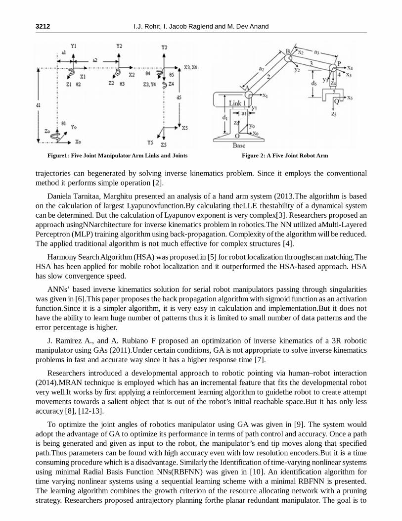
Nowadays robots are considered as an indispensable part of modern manufacturing field with their inherentcapability of executing complex and risky jobs more efficiently and reliably. A robotic manipulator iscomposed of several links connected together through joints. Kinematics deals with the geometric motionof a robotic manipulator and the inverse kinematics is considered as the most popular and efficient methodof controlling robot arm. Figure 1 gives a view of the general structure of a series manipulator with revolutejoints (5 DOF).
The Figure 2 shows a five Degree of Freedom joints related to waist, shoulder, elbow, pitch and roll.
The proposed approach is a strategy that can be implemented to solve the inverse kinematics problemsfaced in robotics with highest DOF more efficiently.
Researchers proposed a Neuro-Genetic Approach to determine the inverse kinematics solution of roboticmanipulators.The proposed solution method is based on using Neural Networks (NN) and Genetic Algorithms(GA) in a hybrid system.Here an Elman NN as well as GA ideas are implemented.The error introduced bythe NN can be minimised by the application of GA. The main problems are the test errors and learning timeis larger and it requires large number of hidden neurons [1].
Adrian-VasileDuka proposed a Novel Approach on NN Based inverse kinematics solution for trajectorytracking of a robotic arm (2011).It employsthe conventional feed forward NN.By using this idea the desired
* PG Student, Department of Aeronautical Engineering, Noorul Islam Centre for Higher Education, Kumaracoil-629 180, Thuckalay,Kanyakumari District, Tamilnadu State, India, Email: [email protected]
** Professor and Deputy Director Research, Department of Electrical and Electronics Engineering, Noorul Islam Centre for HigherEducation, Kumaracoil-629 180, Thuckalay, Kanyakumari District, Tamilnadu State, India, Email: [email protected]
*** Professor and Deputy Director Academic Affairs, Department of Mechanical Engineering, Noorul Islam Centre for Higher Education,Kumaracoil-629 180, Thuckalay, Kanyakumari District, Tamilnadu State, India, Email: [email protected]
ISSN: 0974-5572
3212 I.J. Rohit, I. Jacob Raglend and M. Dev Anand
trajectories can begenerated by solving inverse kinematics problem. Since it employs the conventionalmethod it performs simple operation [2].
Daniela Tarnitaa, Marghitu presented an analysis of a hand arm system (2013.The algorithm is basedon the calculation of largest Lyapunovfunction.By calculating theLLE thestability of a dynamical systemcan be determined. But the calculation of Lyapunov exponent is very complex[3]. Researchers proposed anapproach usingNNarchitecture for inverse kinematics problem in robotics.The NN utilized aMulti-LayeredPerceptron (MLP) training algorithm using back-propagation. Complexity of the algorithm will be reduced.The applied traditional algorithm is not much effective for complex structures [4].
Harmony Search Algorithm (HSA) was proposed in [5] for robot localization throughscan matching.TheHSA has been applied for mobile robot localization and it outperformed the HSA-based approach. HSAhas slow convergence speed.
ANNs’ based inverse kinematics solution for serial robot manipulators passing through singularitieswas given in [6].This paper proposes the back propagation algorithm with sigmoid function as an activationfunction.Since it is a simpler algorithm, it is very easy in calculation and implementation.But it does nothave the ability to learn huge number of patterns thus it is limited to small number of data patterns and theerror percentage is higher.
J. Ramirez A., and A. Rubiano F proposed an optimization of inverse kinematics of a 3R roboticmanipulator using GAs (2011).Under certain conditions, GA is not appropriate to solve inverse kinematicsproblems in fast and accurate way since it has a higher response time [7].
Researchers introduced a developmental approach to robotic pointing via human–robot interaction(2014).MRAN technique is employed which has an incremental feature that fits the developmental robotvery well.It works by first applying a reinforcement learning algorithm to guidethe robot to create attemptmovements towards a salient object that is out of the robot’s initial reachable space.But it has only lessaccuracy [8], [12-13].
To optimize the joint angles of robotics manipulator using GA was given in [9]. The system wouldadopt the advantage of GA to optimize its performance in terms of path control and accuracy. Once a pathis being generated and given as input to the robot, the manipulator’s end tip moves along that specifiedpath.Thus parameters can be found with high accuracy even with low resolution encoders.But it is a timeconsuming procedure which is a disadvantage. Similarly the Identification of time-varying nonlinear systemsusing minimal Radial Basis Function NNs(RBFNN) was given in [10]. An identification algorithm fortime varying nonlinear systems using a sequential learning scheme with a minimal RBFNN is presented.The learning algorithm combines the growth criterion of the resource allocating network with a pruningstrategy. Researchers proposed antrajectory planning forthe planar redundant manipulator. The goal is to
Figure1: Five Joint Manipulator Arm Links and Joints Figure 2: A Five Joint Robot Arm
Inverse Kinematics Solution of a Five Joint Robot Using MRAN Algorithm 3213
minimize the sum of the end-effector position error at each intermediate point along the trajectory whichmakes the end-effector to track the prescribed trajectory accurately for a 3DOF planar manipulator withdifferent end-effector trajectories have been carried out [11].
This paper proposes the neural network idea Minimum Resource Allocation Network algorithm, andhere the algorithms undergo the growing as well as the pruning method to train the network.
2. FORWARD KINEMATIC MODEL OF SCORBOT-ER VU PLUS INDUSTRIAL ROBOT
The answer for the forward kinematics issue comprises of discovering the estimation of the extreme locationof TCP. This result is a capacity of 5 joint qualities, and D-H parameters. There are a few techniques tointensify this issue. This research is carried out utilizing the homogeneous conversion matrices technique,and the D-H’s deliberate representation of the reference frameworks. Despite the fact that the last positionmight be discovered geometrically, the technique proposed in this work offers a reaction which couldcompare the location of the extreme of each connection in the kinematics network, contrasted with the pastor the worldwide standard framework, so as to characterize the position of every explanation in the robot.
2.1. Frame Assignment and Structure
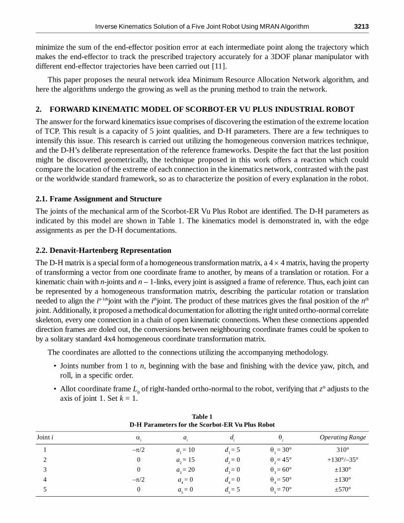
The joints of the mechanical arm of the Scorbot-ER Vu Plus Robot are identified. The D-H parameters asindicated by this model are shown in Table 1. The kinematics model is demonstrated in, with the edgeassignments as per the D-H documentations.
2.2. Denavit-Hartenberg Representation
The D-H matrix is a special form of a homogeneous transformation matrix, a 4 � 4 matrix, having the propertyof transforming a vector from one coordinate frame to another, by means of a translation or rotation. For akinematic chain with n-joints and n – 1-links, every joint is assigned a frame of reference. Thus, each joint canbe represented by a homogeneous transformation matrix, describing the particular rotation or translationneeded to align the in-1thjoint with the ithjoint. The product of these matrices gives the final position of the nth
joint. Additionally, it proposed a methodical documentation for allotting the right united ortho-normal correlateskeleton, every one connection in a chain of open kinematic connections. When these connections appendeddirection frames are doled out, the conversions between neighbouring coordinate frames could be spoken toby a solitary standard 4x4 homogeneous coordinate transformation matrix.
The coordinates are allotted to the connections utilizing the accompanying methodology.
• Joints number from 1 to n, beginning with the base and finishing with the device yaw, pitch, androll, in a specific order.
• Allot coordinate frame L0 of right-handed ortho-normal to the robot, verifying that z° adjusts to the
axis of joint 1. Set k = 1.
Table 1D-H Parameters for the Scorbot-ER Vu Plus Robot
Joint i �i
ai
di
�i
Operating Range
1 –�/2 a1 = 10 d
1 = 5 �
1 = 30° 310°
2 0 a2 = 15 d
2 = 0 �
2 = 45° +130°/–35°
3 0 a3 = 20 d
3 = 0 �
3 = 60° ±130°
4 –�/2 a4 = 0 d
4 = 0 �
4 = 50° ±130°
5 0 a5 = 0 d
5 = 5 �
5 = 70° ±570°
3214 I.J. Rohit, I. Jacob Raglend and M. Dev Anand
• Adjust the axis of joint k + 1 with zk.
• Locate the source of Lk at the crossing point of the zk and zk-1 axis. On the off chance that they don’t
converge, use convergence of zk with a typical ordinary in the middle of zk and zk-1.
• Choose xk to be orthogonal to zk and zk-1 both. In the event that zk and zk-1 are parallel, point xk far from zk-1.
• Choose yk to structure an ortho-normal coordinate outline Lk.
• Make k = k + 1. In the event that k < n, go to step 2; else, proceed.
• Make the starting point of Ln at the device tip. Adjust zn to the methodology vector, yn the sliding
vector, and xn with the typical vector of the tool. Set k = 1.
• Allocate point bk at the convergence of the xk and Zk-1 pivot. In the event that they don’t cross, utilizethe crossing point of xk with a typical ordinary in the middle of xk and zk-1.
• Find �k as the angle of turn from xk-1 to xk measured about zk-1.
• Find dk as the distance from the beginning of frame L
k-1 to point bk, measured along zk-1.
• Find ak as the distance from point bk to the beginning of frame L
k, measured along xk.
• Find �k as the angle of turn from zk-1 to zk measured about xk.
• Set k = k + 1. In the event that k � n, go to step 8; else, stop.
2.3. Transformation Matrix
In the wake of creating the D-H coordinate framework for every connection, a similar matrix of transformationcan without much of a stretch be produced, bearing in mind body{i-1} and body{i} change comprising offour essential conversions. The general complex homogeneous matrix of transformation can be shaped bysequential applications of basic changes. This transformation comprises of four essential conversions.
T1: Angle �
i for z
i-1 axis of rotation
T2: Distance d
i for z
i-1 axis of translation
T3: Distance a
i along x
i axis of translation and
T4: Angle �
i about x
i axis of rotation
Taking into account the D-H gathering, the transformation matrix from joint i to joint i+1 is prearranged by:
1
0
0 0 0 1
ii
C i S iC i S iS i aiC i
S i C iC i C iS i aiS iT
S i C i di (1)
Where S�i = Sin �
i, C�
i = Cos �
i, S�
i = Sin �
i, C�
i = Cos �
i. The Overall Transformation Matrix,
0T5 = 0T
1* 1T
2* 2T
3* 3T
4*4T
5(2)
1 1 1 1
1 1 1 10
1 1
0
0
0 1 0
10 0 0
C S a C
S C a ST d
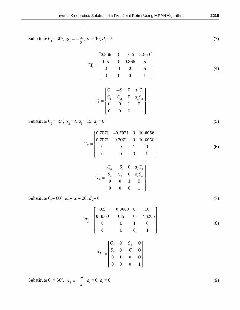
Inverse Kinematics Solution of a Five Joint Robot Using MRAN Algorithm 3215
Substitute �1 = 30°, 1
1
,2
a1 = 10, d
1 = 5 (3)
01
0.866 0 0.5 8.660
0.5 0 0.866 5
0 1 0 5
0 0 0 1
T(4)
2 2 2 2
2 2 2 212
0
0
0 0 1 0
0 0 0 1
C S a C
S C a ST
Substitute �2 = 45°, �
2 = a
2 = 15, d
2 = 0 (5)
12
0.7071 0.7071 0 10.6066
0.7071 0.7071 0 10.6066
0 0 1 0
0 0 0 1
T(6)
3 3 3 3
3 3 3 323
0
0
0 0 1 0
0 0 0 1
C S a C
S C a ST
Substitute �3= 60°, �
3 = a
3 = 20, d
3 = 0 (7)
23
0.5 0.8660 0 10
0.8660 0.5 0 17.3205
0 0 1 0
0 0 0 1
T(8)
4 4
4 434
0 0
0 0
0 1 0 0
0 0 0 1
C S
S CT
Substitute �4 = 50°,
4 ,2
a4 = 0, d
4 = 0 (9)
3216 I.J. Rohit, I. Jacob Raglend and M. Dev Anand
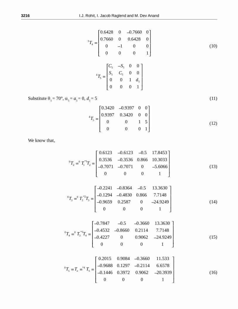
34
0.6428 0 0.7660 0
0.7660 0 0.6428 0
0 1 0 0
0 0 0 1
T(10)
5 5
5 545
5
0 0
0 0
0 0 1
0 0 0 1
C S
S CT
d
Substitute �5 = 70°, �
5 = a
5 = 0, d
5 = 5 (11)
45
0.3420 0.9397 0 0
0.9397 0.3420 0 0
0 0 1 5
0 0 0 1
T(12)
We know that,
*10 02 1 2
0.6123 0.6123 0.5 17.8453
0.3536 0.3536 0.866 10.3033
0.7071 0.7071 0 5.6066
0 0 0 1
T T T(13)
*20 03 2 3
0.2241 0.8364 0.5 13.3630
0.1294 0.4830 0.866 7.7148
0.9659 0.2587 0 24.9249
0 0 0 1
T T T(14)
*30 04 3 4
0.7847 0.5 0.3660 13.3630
0.4532 0.8660 0.2114 7.7148
0.4227 0 0.9062 24.9249
0 0 0 1
T T T(15)
0 *45 5
0.2015 0.9084 0.3660 11.533
0.9688 0.1297 0.2114 6.6578
0.1446 0.3972 0.9062 20.3939
0 0 0 1
eT T T(16)
Inverse Kinematics Solution of a Five Joint Robot Using MRAN Algorithm 3217
2.4. VERIFICATION OF THE MODEL BY MATLAB
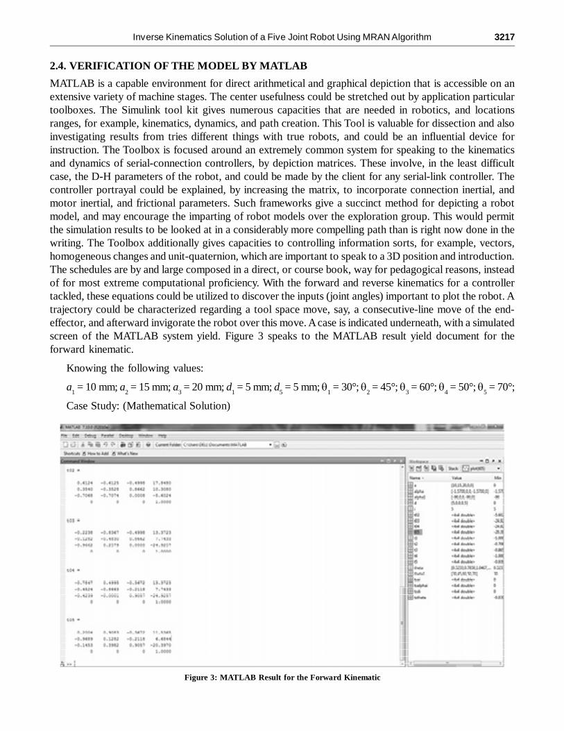
MATLAB is a capable environment for direct arithmetical and graphical depiction that is accessible on anextensive variety of machine stages. The center usefulness could be stretched out by application particulartoolboxes. The Simulink tool kit gives numerous capacities that are needed in robotics, and locationsranges, for example, kinematics, dynamics, and path creation. This Tool is valuable for dissection and alsoinvestigating results from tries different things with true robots, and could be an influential device forinstruction. The Toolbox is focused around an extremely common system for speaking to the kinematicsand dynamics of serial-connection controllers, by depiction matrices. These involve, in the least difficultcase, the D-H parameters of the robot, and could be made by the client for any serial-link controller. Thecontroller portrayal could be explained, by increasing the matrix, to incorporate connection inertial, andmotor inertial, and frictional parameters. Such frameworks give a succinct method for depicting a robotmodel, and may encourage the imparting of robot models over the exploration group. This would permitthe simulation results to be looked at in a considerably more compelling path than is right now done in thewriting. The Toolbox additionally gives capacities to controlling information sorts, for example, vectors,homogeneous changes and unit-quaternion, which are important to speak to a 3D position and introduction.The schedules are by and large composed in a direct, or course book, way for pedagogical reasons, insteadof for most extreme computational proficiency. With the forward and reverse kinematics for a controllertackled, these equations could be utilized to discover the inputs (joint angles) important to plot the robot. Atrajectory could be characterized regarding a tool space move, say, a consecutive-line move of the end-effector, and afterward invigorate the robot over this move. A case is indicated underneath, with a simulatedscreen of the MATLAB system yield. Figure 3 speaks to the MATLAB result yield document for theforward kinematic.
Knowing the following values:
a1 = 10 mm; a
2 = 15 mm; a
3 = 20 mm; d
1 = 5 mm; d
5 = 5 mm; �
1 = 30°; �
2 = 45°; �
3 = 60°; �
4 = 50°; �
5 = 70°;
Case Study: (Mathematical Solution)
Figure 3: MATLAB Result for the Forward Kinematic
3218 I.J. Rohit, I. Jacob Raglend and M. Dev Anand
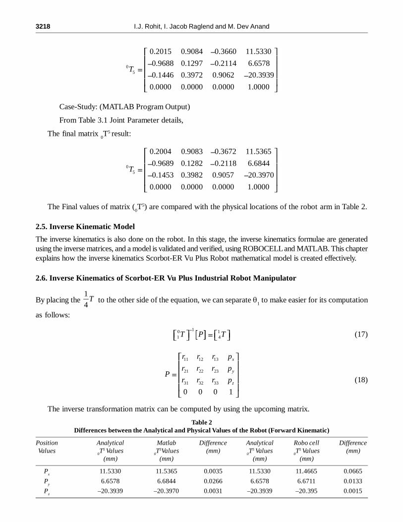
05
0.2015 0.9084 0.3660 11.5330
0.9688 0.1297 0.2114 6.6578
0.1446 0.3972 0.9062 20.3939
0.0000 0.0000 0.0000 1.0000
T
Case-Study: (MATLAB Program Output)
From Table 3.1 Joint Parameter details,
The final matrix 0T5 result:
05
0.2004 0.9083 0.3672 11.5365
0.9689 0.1282 0.2118 6.6844
0.1453 0.3982 0.9057 20.3970
0.0000 0.0000 0.0000 1.0000
T
The Final values of matrix (0T5) are compared with the physical locations of the robot arm in Table 2.
2.5. Inverse Kinematic Model
The inverse kinematics is also done on the robot. In this stage, the inverse kinematics formulae are generatedusing the inverse matrices, and a model is validated and verified, using ROBOCELL and MATLAB. This chapterexplains how the inverse kinematics Scorbot-ER Vu Plus Robot mathematical model is created effectively.
2.6. Inverse Kinematics of Scorbot-ER Vu Plus Industrial Robot Manipulator
By placing the 1
4T to the other side of the equation, we can separate �
1 to make easier for its computation
as follows:
10 11 4T P T (17)
11 12 13
21 22 23
31 32 33
0 0 0 1
x
y
z
r r r p
r r r pP
r r r p (18)
The inverse transformation matrix can be computed by using the upcoming matrix.
Table 2Differences between the Analytical and Physical Values of the Robot (Forward Kinematic)
Position Analytical Matlab Difference Analytical Robo cell DifferenceValues
0T5 Values
0T5Values (mm)
0T5 Values
0T5 Values (mm)
(mm) (mm) (mm) (mm)
Px
11.5330 11.5365 0.0035 11.5330 11.4665 0.0665
Py
6.6578 6.6844 0.0266 6.6578 6.6711 0.0133
Pz
–20.3939 –20.3970 0.0031 –20.3939 –20.395 0.0015
Inverse Kinematics Solution of a Five Joint Robot Using MRAN Algorithm 3219
1
0 1
T TR R PT (19)
Applying this to yields the following result,
1 1
1 1 101
1
0 0
0 0
0 0 1
0 0 0 1
C S
S CT
d (20)
Therefore,
1 1 11 12 13
1 1 21 22 23
1 31 32 33
0 0
0 0
0 0 1
0 0 0 1 0 0 0 1
x
y
z
C S r r r p
S C r r r p
d r r r p
23 23 1 2 2 3 23
1 1 2
2 2 3 23
0
0
0 0 1
0 0 0 1
C S a a C a C
S C d
a S a S (21)
For compute �1 the element (2, 4) in the matrix can be utilized.
2 1 1sin cosx yd p p (22)
Letting,
cosxp (23)
sinyp (24)
Where,
2 2x yp p (25)
� = Arctan 2 (py, p
x) (26)
We know that,
21 1sin cos cos sin
d(27)
Therefore,
21sin
d(28)
22
1 2cos 1d
(29)
22 2
1 2arctan 2 , 1d d
(30)
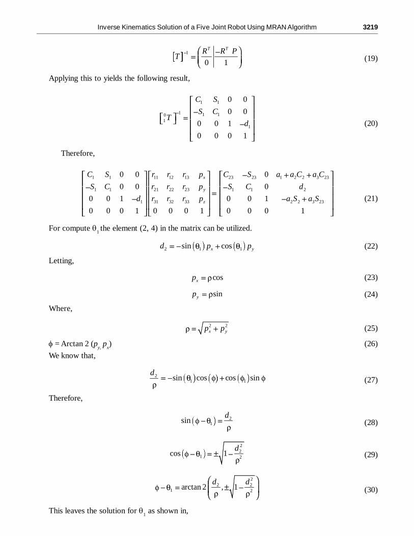
This leaves the solution for �1 as shown in,
3220 I.J. Rohit, I. Jacob Raglend and M. Dev Anand
�1 = arctan 2 (p
y, p
x) -arctan 2 2 2 2
2 2, x yd p p d (31)
For compute the joint angle three, we must verify the elements from (1, 4) and (3, 4). First,
C1 p
x + S
1 p
y = a
3 C
23 + a
2 C
2 + a
1(32)
pz – d
1 = –a
3 S
23 – a
2 S
2(33)
Next by squaring Equation (32) and Equation (33) followed by addition, �3 can be determined.
(C1
px + S
1 p
y –a
1)2 + (d
1 – p
z)2 = (a
3 C
23 + a
2 C
2)2 + (a
3 S
23 + a
2 S
2)2 (34)
(C1
px + S
1 p
y –a
1)2 + (d
1 – p
z)2 2 2
2 3 2 3 2 23 2 232 ( )a a a a C C S S (35)
(C1
px + S
1 p
y –a
1)2 + (d
1 – p
z)2 2 2
2 3 2 3 32 a a a a C (36)
This leaves Equation (3.37) for �3,
2 2 2 21 1 1 1 2 3
32 3
arccos2
x y zC p S p a d p a a
a a (37)
Next by transferring the matrix 12T onto the other side, next equation can be found that will permit us
to find �2.
1 11 0 22 1 4T T P T (38)
2 2 1 2
1 2 2 2 212
2
0
0
0 1 0
0 0 0 1
C S a C
S C a ST
d (39)
2 2 1 2 1 1
1 1 2 2 1 2 1 11 02 1
2 1
0 0 0
0 0 0
0 1 0 0 0 1
0 0 0 1 0 0 0 1
C S a C C S
S C a S S CT T
d d (40)
1 2 1 2 2 2 1 1 2
1 1 1 2 1 2 2 2 1 1 21 02 1
1 1 20
0 0 0 1
C C S C S S d a C
C S S S C C d a ST T
S C d (41)
1 2 1 2 2 2 1 1 2 11 12 13 3 3 3 3 2
1 2 1 2 2 2 1 1 2 21 22 23 3 3 3 3
1 1 2 31 32 33
0
0
0 0 0 1 0
0 0 0 1 0 0 0 1 0 0 0 1
x
y
z
C C S C S S d a C r r r p C S a C a
C S S S C C d a S r r r p S C a S
S C d r r r p (42)
Inverse Kinematics Solution of a Five Joint Robot Using MRAN Algorithm 3221
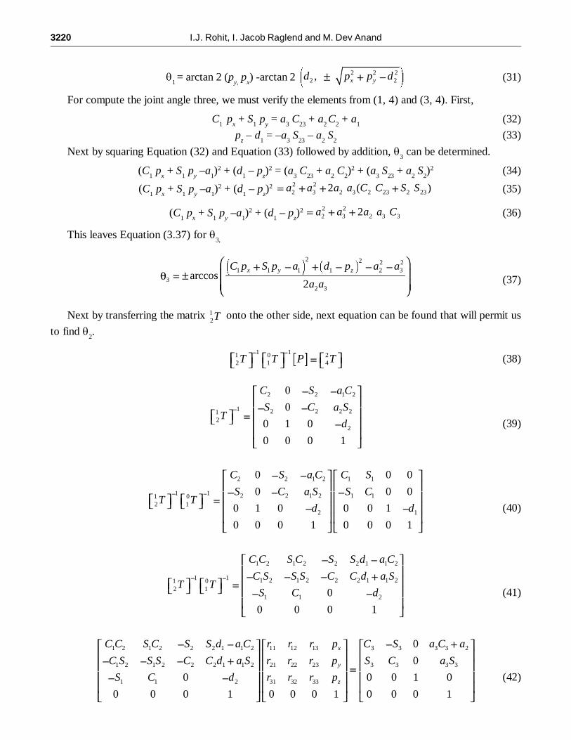
By finding elements (1, 4) of the above Equation (42) we stick with the following formula.
C1
C2
px + S
1 C
2 p
y – S
2 p
z + d
1 S
2– C
2 a
1 = a
3 C
3 + a
2(43)
C2
(C1
px + S
1 p
y – a
1) + S
2 (d
1 – p
z)
= a
3 C
3 + a
2(44)
Substituting A = (C1
px + S
1 p
y – a
1) B = (d
1 – p
z)
and C = a
3 C
3 + a
2 it is easy to solve �
2 via reduction
to a polynomial.
C2A + S
2B = C (45)
Where,
2
2 2
1
1
UC
U(46)
2 2
2
1
US
U(47)
Substituting the above two Equation (3.46) and Equation (3.47) into Equation (3.45) and rearranging,Equation (3.48) is obtained.
(C + A)U2 – 2UB + (C – A) (48)
The quadratic formula rendering can be used to solve this:
2 2 2B B A CU
A C(49)
Where �
�2 = 2 arctan (U) (50)
The angle of the 4th joint, �4, can also be simply determined, based on �
2 and �
3.
4z zp p a (51)
�4 = 90 – �
2 – �
3(52)
Replace the z offset in Equation (3.49), we find the upcoming set of formulae for the inverse kinematicsof the Scorbot-ER Vu Plus Robot.
�1 = arctan 2 (p
y, p
x) arctan 2 2 2 2
2 2, x yd p p d (53)
2 2 2 21 1 1 1 4 2 3
32 32
x y zC p S p a d p a a aarccos
a a (54)
22 2
1 4 1 4 1 1 1 3 3 2
2
1 1 1 3 3 2
2z z x y
x y
d p a d p a c p S p a a C aarcta
c p S p a a c a (55)
�4 = 90 – �
2 – �
3(56)
Although in this case �5 was never changed, by substituting all the values of Table 3.1, in the above
formulae, the values can be found.
3222 I.J. Rohit, I. Jacob Raglend and M. Dev Anand
2.7. Verification of the Model by MATLAB and ROBOCELL
ROBOCELL Software is used to validate the Inverse Kinematic Model of the Scorbot-ER Vu Plus IndustrialRobot.
2.7.1. Components of ROBOCELL
ROBOCELL software coordinates the four segments:
i. SCORBASE, full-emphasized robotics control programming software, which gives an easy to usedevice for robot programming and process.
ii. A module with graphic exhibit that provides robot’s 3D dissection of the robot and different gadgetsin a fundamental robotic environment, where one can characterize (instruct) the robot movementsand accomplish robot programs.
iii. Cell setup, which permits a user to make another virtual automated workcell, or change a currentworkcell.
iv. 3D simulation software display to exhibit ROBOCELL’s capacities.
v. ROBOCELL’s illustration of a robot and gadgets is focused around the genuine measurementsand capacities of the Scorbot-ER Vu Plus Robot equipment. In this way, working and programmingthe robot in ROBOCELL could be utilized with a genuine robotic establishment. Realisticpresentation peculiarities and programmed operations, for example, cell reset and send robotcommands, empower fast and exact programming. SCORBASE’s imitate the client interface andmenus of ROBOCELL. SCORBASE operations, menus and commands are depicted in theSCORBASE hand book.
vi. ROBOCELL gives the strategies depicted beneath, for characterizing the positions of the robot.Allotted number indicates its position.
2.7.2. Recording Position (First Method)
i. The virtual robot is controlled by the SCORBASE physical dialog box like a real robot.
ii. In the teach position (Simple) dialog box a number is written in the location number field when theposition is reached.
iii. Click the record button.
iv. The new position will replace the existence position data in the event that the position number hasbeen utilized long ago.
2.7.3. Recording Position (Second Method)
i. Position and above position tools are used for specific location of robot, while robot moves toobject.
ii. Calibration is done by utilizing the manual movement dialog box.
iii. Until the position is reached, location number field’s in the teach position (Simple) dialog box iswritten.
iv. Click the record button.
v. In the event that the position number has been utilized at one time, the new position will overwritethe past position information.
Inverse Kinematics Solution of a Five Joint Robot Using MRAN Algorithm 3223
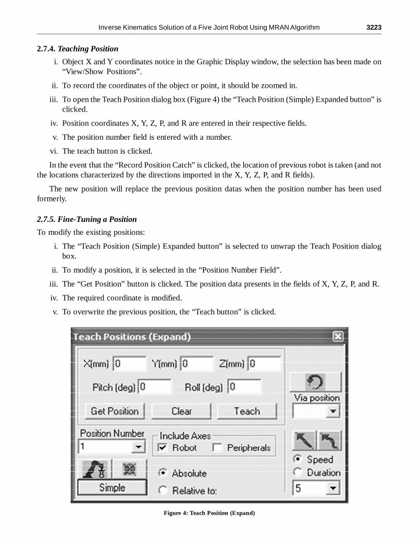
2.7.4. Teaching Position
i. Object X and Y coordinates notice in the Graphic Display window, the selection has been made on“View/Show Positions”.
ii. To record the coordinates of the object or point, it should be zoomed in.
iii. To open the Teach Position dialog box (Figure 4) the “Teach Position (Simple) Expanded button” isclicked.
iv. Position coordinates X, Y, Z, P, and R are entered in their respective fields.
v. The position number field is entered with a number.
vi. The teach button is clicked.
In the event that the “Record Position Catch” is clicked, the location of previous robot is taken (and notthe locations characterized by the directions imported in the X, Y, Z, P, and R fields).
The new position will replace the previous position datas when the position number has been usedformerly.
2.7.5. Fine-Tuning a Position
To modify the existing positions:
i. The “Teach Position (Simple) Expanded button” is selected to unwrap the Teach Position dialogbox.
ii. To modify a position, it is selected in the “Position Number Field”.
iii. The “Get Position” button is clicked. The position data presents in the fields of X, Y, Z, P, and R.
iv. The required coordinate is modified.
v. To overwrite the previous position, the “Teach button” is clicked.
Figure 4: Teach Position (Expand)
3224 I.J. Rohit, I. Jacob Raglend and M. Dev Anand
2.7.6. Program Execution
ROBOCELL project execution is the similar as performing project while utilizing a genuine robot framework.Diverse cell arrangements might be stacked and changed in ROBOCELL. Be that as it may the positionsand projects are not stacked together with their work cell. For another task, to consider the work cell and itspositions, the Save as choice in the File menu might be utilized. The undertaking with work cell andpositions is spared under an alternate name. At that point the project is erased and another one is composed.(The positions and the cell stay unaltered).
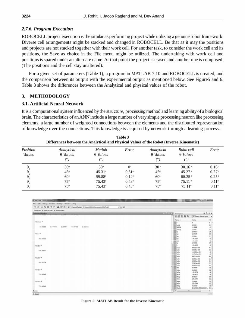
For a given set of parameters (Table 1), a program in MATLAB 7.10 and ROBOCELL is created, andthe comparison between its output with the experimental output as mentioned below. See Figure5 and 6.Table 3 shows the differences between the Analytical and physical values of the robot.
3. METHODOLOGY
3.1. Artificial Neural Network
It is a computational system influenced by the structure, processing method and learning ability of a biologicalbrain. The characteristics of an ANN include a large number of very simple processing neuron like processingelements, a large number of weighted connections between the elements and the distributed representationof knowledge over the connections. This knowledge is acquired by network through a learning process.
Table 3Differences between the Analytical and Physical Values of the Robot (Inverse Kinematic)
Position Analytical Matlab Error Analytical Robo cell ErrorValues � Values � Values � Values � Values
(°) (°) (°) (°)
�1
30o 30o 0o 30 o 30.16 o 0.16 o
�2
45o 45.31o 0.31o 45o 45.27 o 0.27 o
�3
60o 59.88o 0.12o 60o 60.25 o 0.25 o
�4
75o 75.43o 0.43o 75o 75.11 o 0.11o
�5
75o 75.43o 0.43o 75o 75.11o 0.11o
Figure 5: MATLAB Result for the Inverse Kinematic
Inverse Kinematics Solution of a Five Joint Robot Using MRAN Algorithm 3225
3.2. Minimal Resource Allocation Network (MRAN)
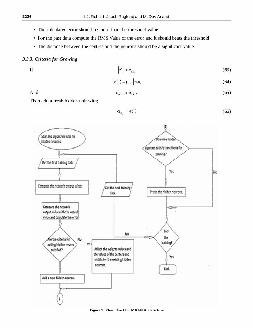
MRAN is minimal radial basis function which is mostly employed in sequential data and it provide thisRBF network only by adding and removing the hidden neurons based on the input and can be adopted foronline adaptive control of time varying nonlinear system The three main steps of MRAN network are (i).Basic error computing (ii). Criteria for adding hidden units (iii). criteria for adding pruning units. Learningwith a fixed size of network will be vague. The networks learning can be increased by increasing or decreasingthe network size. The flow chart for the proposed algorithm is given in Figure 7.
3.2.1. Basic Error Computing
For each input x(i), compute:
2
2
1expk k
k
x i x i (57)
0 1ˆ , ,kNk K Ky i f x i i x i (58)
�i = max{�
max �i, �
min}, (0 < � < 1) (59)
ˆ( ) ( ) ( ),e i y i y i (60)
1ˆ ˆ
Tij i nw
rmsi
y j y j y j y je
nw(61)
In the MRAN algorithm, when the network begins there will be zero hidden neurons. As certain trainingsteps over, the modifications in the network is built up based on certain growing method.It is achieved onlyby satisfying certain conditions. The algorithm adds or prunes hidden units as well as adjusting the existingnetwork parameters to maintain the input output behaviour. A brief outline of the steps like adding andpruning in the MRAN is given below.
3.2.2. Steps for Adding Hidden Units
Step 1 Collect the input X, and compute the result
Step 2 Generate the new hidden unit if and only if the successive conditions are satisfied
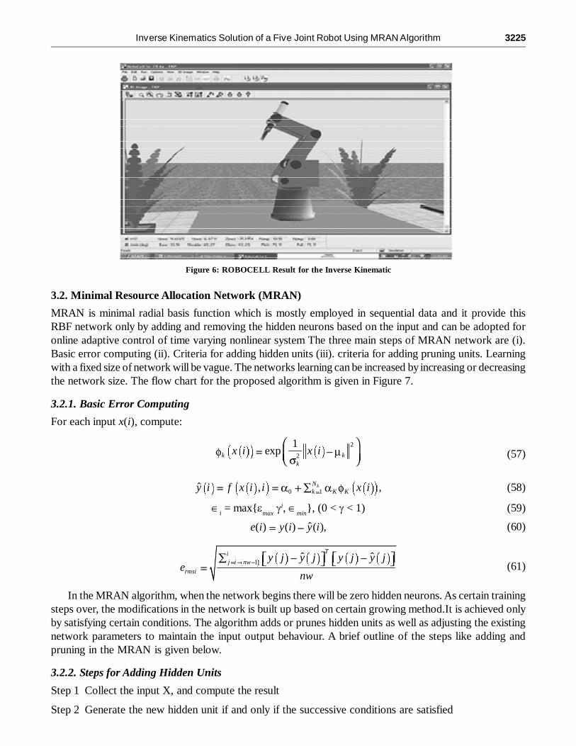
Figure 6: ROBOCELL Result for the Inverse Kinematic
3226 I.J. Rohit, I. Jacob Raglend and M. Dev Anand
• The calculated error should be more than the threshold value
• For the past data compute the RMS Value of the error and it should beats the threshold
• The distance between the centres and the neurons should be a significant value.
3.2.3. Criteria for Growing
If minie e (63)
nr ix i (64)
And ,rmsi mine e (65)
Then add a fresh hidden unit with;
( )hN e i (66)
Figure 7: Flow Chart for MRAN Architecture
Inverse Kinematics Solution of a Five Joint Robot Using MRAN Algorithm 3227
( )hN x i (67)
hN nrk x i (68)
Else wi = w
i–1 + K
ie(i) (69)
1
1 1 ,Ti i i i i iK P A V A TP A (70)
1 0T
i i i iP I K A P q I (71)
Step-3. If the conditions in Step 2 are not met, adjust the weights and widths of the existing RBFnetwork using an extended KalmanFilter (EKF).
3.2.4. Steps for Adding Pruning Units
Pruning means the least useful nodes and weights are iteratively removed and adjusted to maintain theoriginal i/p o/p behavior. Some of the steps involved in pruning strategy is given as;
For every observation (Xn, Yn), compute the outputs of hidden unit so ,i
k (k = 1, ……, Nh)
Find the largest absolute hidden unit output value and Compute the normalized output values for allhidden units
,max ,max ,max ,max,..., ,...,T
i i i iI I I Po o o o (72)
Calculate the normalized output vector ik for each hidden unit in which the kth element is expressed as
,max
, 1, ...... , 1...i
i IKk hi
I
oK N I p
o (73)
If the values of all elements in ik are less then � for the consecutive observations, then prune the k
hidden units.
The flow chart makes us understand the MRAN algorithm clearly. The algorithm begins with no hiddenneurons. As time elapses the hidden units are added and are based on certain conditions. After starting thenetwork, the training data is obtained and compute the network output values aswell as the error betweenthe actual value and the obtained value.Then we put forward certain criteria and if its satisfies the additionof new neuron takes place. If some neurons satisfies the pruning criteria the removing of hidden units takesplace. Thus by adding and pruning the adjustments can be made to maintain the input output behaviour.
4. RESULT AND DISCUSSION
The positions and orientation corresponding to the Cartesian coordinate system has been analyzed byemploying the MRAN algorithms by using a set of joint angles as targets. The network got trained using thegiven input parameter values and can be simulated using MATLAB software. The mean square errorestimation by the program also gives the performance and later it can be analyzed. The performance isplotted by the function mean square error across the number of iterations.
Since considering the inverse kinematics, in this work, the Cartesian coordinates X (150,320), Y (0,150)and Z (-24,505) are given as inputs and �
1(0,45), �
2(-120,43), �
3(20,108),
�
4(-3,89),
�
5(0,70) are the angles
between the inputs and joints which is called target angles. There are three inputs and five outputs and the
3228 I.J. Rohit, I. Jacob Raglend and M. Dev Anand
goal is to obtain a minimum mean square error which means a performance algorithm. The positions andorientation based on the Cartesian coordinate system has been analysed by employing the artificial neuralnetwork method, MRAN by using a set of joint angles as desired output. The network got trained usingdifferent parameter values and can be simulated using MATLAB software. The program also gives themean square error by which the performance can be analysed.
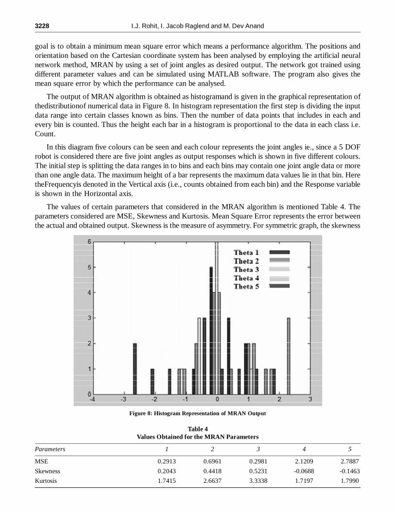
The output of MRAN algorithm is obtained as histogramand is given in the graphical representation ofthedistributionof numerical data in Figure 8. In histogram representation the first step is dividing the inputdata range into certain classes known as bins. Then the number of data points that includes in each andevery bin is counted. Thus the height each bar in a histogram is proportional to the data in each class i.e.Count.
In this diagram five colours can be seen and each colour represents the joint angles ie., since a 5 DOFrobot is considered there are five joint angles as output responses which is shown in five different colours.The initial step is splitting the data ranges in to bins and each bins may contain one joint angle data or morethan one angle data. The maximum height of a bar represents the maximum data values lie in that bin. HeretheFrequencyis denoted in the Vertical axis (i.e., counts obtained from each bin) and the Response variableis shown in the Horizontal axis.
The values of certain parameters that considered in the MRAN algorithm is mentioned Table 4. Theparameters considered are MSE, Skewness and Kurtosis. Mean Square Error represents the error betweenthe actual and obtained output. Skewness is the measure of asymmetry. For symmetric graph, the skewness
Figure 8: Histogram Representation of MRAN Output
Table 4Values Obtained for the MRAN Parameters
Parameters 1 2 3 4 5
MSE 0.2913 0.6961 0.2981 2.1209 2.7887
Skewness 0.2043 0.4418 0.5231 -0.0688 -0.1463
Kurtosis 1.7415 2.6637 3.3338 1.7197 1.7990
Inverse Kinematics Solution of a Five Joint Robot Using MRAN Algorithm 3229
value will be zero. If the value will be positive, then it shows the distribution extents more to the right halfof the graph and negative skewness shows the distributions more in the left half. Kurtosis is the factorwhich shows the measure of peaked values.
5. CONCLUSION
This work formulates and simulates the solution for the inverse kinematic problem of a five DOF robot isobtained using the intelligent technique, ANN and can be analyzed by the performances of the adoptedMRAN algorithm. For improving the accuracy of the predicted joint and link angles, the number of inputpatterns of various coordinate values to be trained can also be increased.
REFERENCES[1] Rasit Koker, “A Neuro-Genetic Approach to the Inverse Kinematics Solution of Robotic Manipulators”, Scientific Research
and Essays, Vol. 6, No. 13, pp. 2784-2794, 2011.
[2] Adrian-VasilebDuka, Neural Network Based Inverse Kinematics Solution for Trajectory Tracking of a Robotic Arm,International Conference on Computer Engineering and Applications, Vol. 2, 2011.
[3] Daniel TarnitaA, Dan B. Marghitu, Analysis of a Hand Arm System, Robotics and Computer-Integrated Manufacturing,Vol. 29, pp. 493–501, 2013.
[4] BassamDaya, ShadiKhawandi, Mohamed Akoum, Applying Neural Network Architecture for Inverse Kinematics Problemin Robotics, Journal Software Engineering & Applications, Vol. 3, pp. 230-239, 2010.
[5] Moshan Mirkhani, Rana Forsati, Alireza Mohammed Shari, A Novel Efficient Algorithm for Mobile Robot Localization,International Journal of Robotics and Autonomous, Vol. 61, pp. 920-931, 2013.
[6] Ali T. Hasan1, Hayder M.A.A. Al-Assadi and Ahmad Azlan Mat Isa, Neural Networks’ Based Inverse Kinematics Solutionfor Serial Robot Manipulators Passing Through Singularities, Artificial Neural Networks-Industrial and Control EngineeringApplications, pp. 459-478.
[7] Ramirez A., and A. Rubiano. F., Optimization of Inverse Kinematics of a 3R Robotic Manipulator Using Genetic AlgorithmsWorld Academy of Science, Engineering and Technology, Vol. 59, 2011.
[8] Fei Chao a, Zhengshuai Wang a, Changjing Shang b, A Developmental Approach to Robotic Pointing via Human–RobotInteraction, 2013.
[9] F.Y.C. Albert, S.P. Koh, C.P. Chen, S.K.Tiong, S.Y.S. Edwin, Optimizing Joint Angles of Robotic Manipulator UsingGenetic Algorithm, International Conference on Computer Engineering and Applications, Vol. 2, 2011.
[10] R. Koker, C. Oz, T. Çakar, and H. Ekiz, A Study of Neural Network Based Inverse Kinematics Solution for a Three-JointRobot, Robotics and Autonomous Systems, Vol. 49, pp. 227–234, 2004.
[11] A.A.Ata, T.R.Myo, Optimal PointtoPoint Trajectory Tracking of Redundant Manipulators Using Generalized PatternSearch, International Journal of Advanced Robotic Systems, Vol. 2, No. 3, pp. 239-244, 2005.
[12] L. Yingwei, N. Sundararajan, P. Saratchandran’ Identification of Time-Varying Nonlinear Systems Using Minimal RadialBasis Function Neural Networks’IEE Proceedings-Control Theory and Applications, Vol. 44, No. 2, pp. 202-208.
[13] Yingwei, L., Sundararajan, N., and Saratchandran, P.: “A Sequential Learning Scheme for Function Approximation UsingMinimal Radial Basis Function Neural Networks’.Technical Report CSP/9505, CenterFor Signal Processing, School ofElectrical and Electronic Engineering, Nanyang Technological University, November 1995.


![In a research on how to use inverse kinematics solution of ...€¦ · [9] Bingül Z, Ertunç HM, Oysu C. Comparison of Inverse Kinematics Solutions Using Neural Network for 6R Robot](https://static.fdocuments.net/doc/165x107/5f7638d9e0937d6f87619ede/in-a-research-on-how-to-use-inverse-kinematics-solution-of-9-bingl-z-ertun.jpg)


