Inverse Kinematics (part 2)

CSE169: Computer Animation

Instructor: Steve Rotenberg

UCSD, Winter 2004

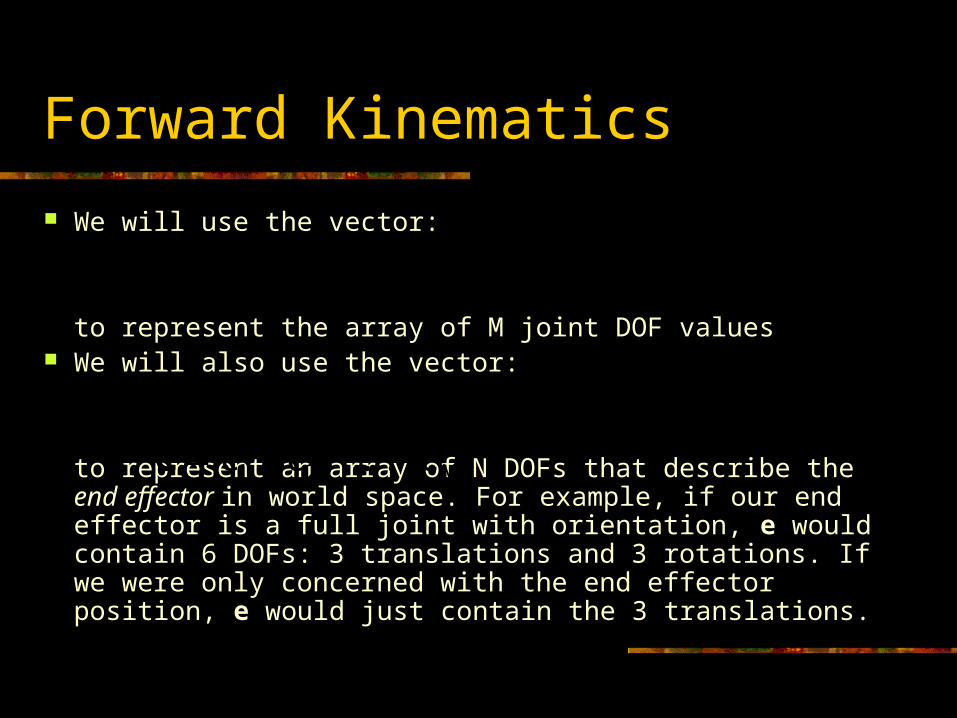
Forward Kinematics

We will use the vector:

to represent the array of M joint DOF values We will also use the vector:

to represent an array of N DOFs that describe the end effector in world space. For example, if our end effector is a full joint with orientation, e would contain 6 DOFs: 3 translations and 3 rotations. If we were only concerned with the end effector position, e would just contain the 3 translations.

M ...21Φ

Neee ...21e

Forward & Inverse Kinematics

The forward kinematic function computes the world space end effector DOFs from the joint DOFs:

The goal of inverse kinematics is to compute the vector of joint DOFs that will cause the end effector to reach some desired goal state

Φe f

eΦ 1 f

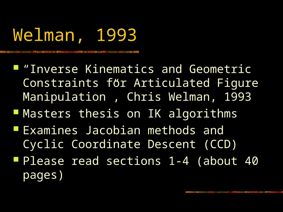
Welman, 1993

“Inverse Kinematics and Geometric Constraints for Articulated Figure Manipulation”, Chris Welman, 1993

Masters thesis on IK algorithms Examines Jacobian methods and Cyclic

Coordinate Descent (CCD) Please read sections 1-4 (about 40 pages)

Gradient Descent

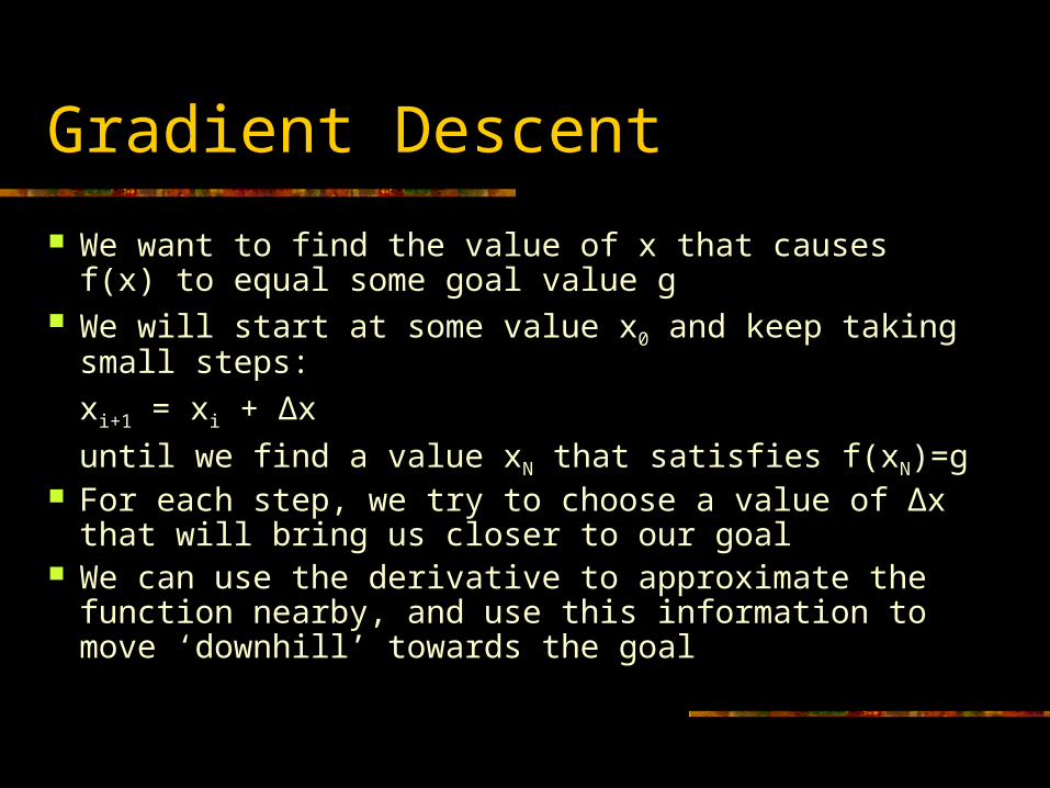
We want to find the value of x that causes f(x) to equal some goal value g

We will start at some value x0 and keep taking small steps:

xi+1 = xi + Δx

until we find a value xN that satisfies f(xN)=g For each step, we try to choose a value of Δx that will

bring us closer to our goal We can use the derivative to approximate the function

nearby, and use this information to move ‘downhill’ towards the goal

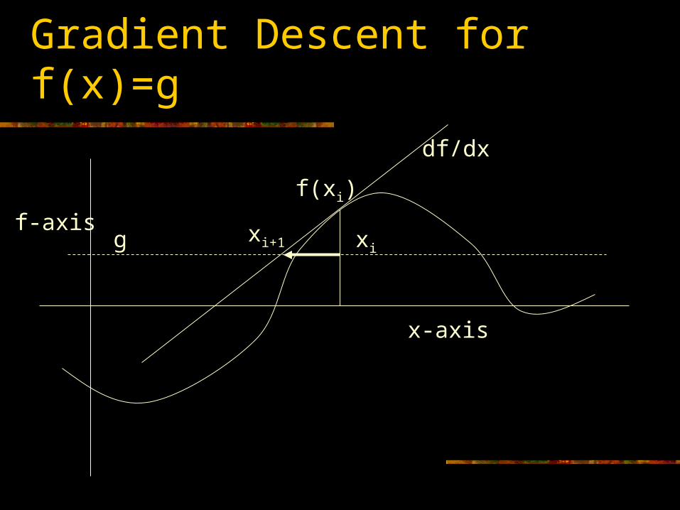
Gradient Descent for f(x)=g

f-axis

x-axis

xi

f(xi)

df/dx

g xi+1

Minimization

If f(xi)-g is not 0, the value of f(xi)-g can be thought of as an error. The goal of gradient descent is to minimize this error, and so we can refer to it as a minimization algorithm

Each step Δx we take results in the function changing its value. We will call this change Δf.

Ideally, we could have Δf = g-f(xi). In other words, we want to take a step Δx that causes Δf to cancel out the error

More realistically, we will just hope that each step will bring us closer, and we can eventually stop when we get ‘close enough’

This iterative process involving approximations is consistent with many numerical algorithms

Taking Safe Steps

Sometimes, we are dealing with non-smooth functions with varying derivatives

Therefore, our simple linear approximation is not very reliable for large values of Δx

There are many approaches to choosing a more appropriate (smaller) step size

One simple modification is to add a parameter β to scale our step (0≤ β ≤1)

1

dx

dfxfgx i

Inverse of the Derivative

By the way, for scalar derivatives:

df

dx

dxdfdx

df

1

1

Gradient Descent Algorithm

}

newat evaluate //

along step // take1

slope compute/ /

{ while

at evaluate //

valuestarting initial

111

1

000

0

iii

iiii

ii

n

xfxff

xs

fgxx

xdx

dfs

gf

xfxff

x

Jacobians

A Jacobian is a vector derivative with respect to another vector

If we have a vector valued function of a vector of variables f(x), the Jacobian is a matrix of partial derivatives- one partial derivative for each combination of components of the vectors

The Jacobian matrix contains all of the information necessary to relate a change in any component of x to a change in any component of f

The Jacobian is usually written as J(f,x), but you can really just think of it as df/dx

Jacobians

N

MM

N

x

f

x

f

x

f

x

fx

f

x

f

x

f

d

dJ

......

............

......

...

,

1

2

2

1

2

1

2

1

1

1

x

fxf

Jacobian Inverse Kinematics

Jacobians

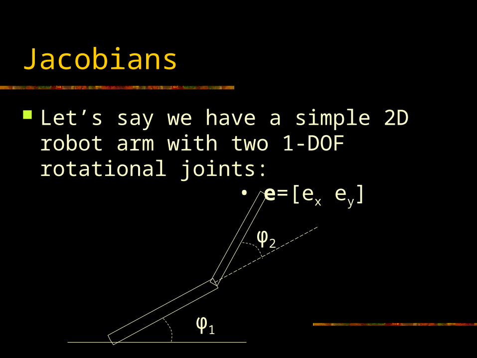
Let’s say we have a simple 2D robot arm with two 1-DOF rotational joints:

φ1

φ2

• e=[ex ey]

Jacobians

The Jacobian matrix J(e,Φ) shows how each component of e varies with respect to each joint angle

21

21,

yy

xx

ee

ee

J Φe

Jacobians

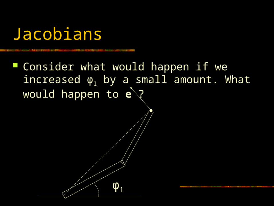
Consider what would happen if we increased φ1 by a small amount. What would happen to e ?

φ1

•

111 yxeee

Jacobians

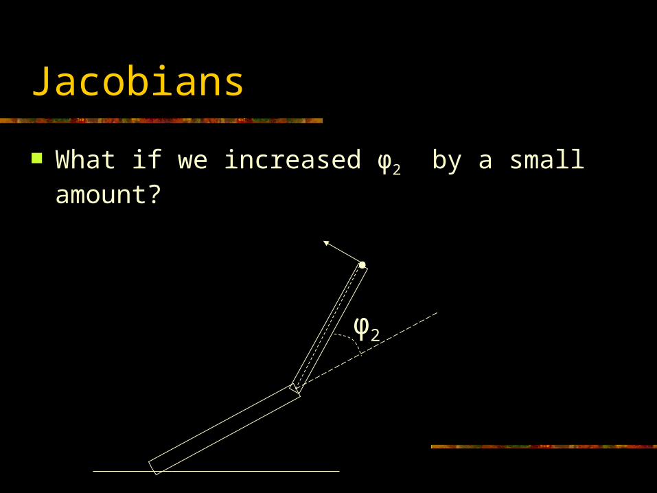
What if we increased φ2 by a small amount?

φ2

•

222 yxeee

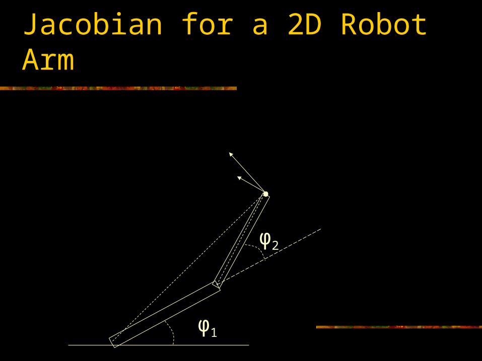
Jacobian for a 2D Robot Arm

φ2

•

φ1

21

21,

yy

xx

ee

ee

J Φe

Jacobian Matrices

Just as a scalar derivative df/dx of a function f(x) can vary over the domain of possible values for x, the Jacobian matrix J(e,Φ) varies over the domain of all possible poses for Φ

For any given joint pose vector Φ, we can explicitly compute the individual components of the Jacobian matrix

Incremental Change in Pose

Lets say we have a vector ΔΦ that represents a small change in joint DOF values

We can approximate what the resulting change in e would be:

ΦJΦΦeΦΦ

ee ,Jd

d

Incremental Change in Effector

What if we wanted to move the end effector by a small amount Δe. What small change ΔΦ will achieve this?

eJΦ

ΦJe

1

: so

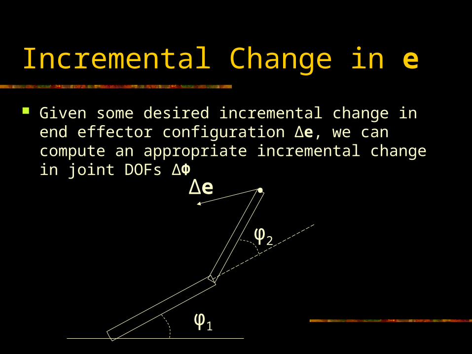
Incremental Change in e

φ2

•

φ1

eJΦ 1

Δe

Given some desired incremental change in end effector configuration Δe, we can compute an appropriate incremental change in joint DOFs ΔΦ

Incremental Changes

Remember that forward kinematics is a nonlinear function (as it involves sin’s and cos’s of the input variables)

This implies that we can only use the Jacobian as an approximation that is valid near the current configuration

Therefore, we must repeat the process of computing a Jacobian and then taking a small step towards the goal until we get to where we want to be

Choosing Δe

We want to choose a value for Δe that will move e closer to g. A reasonable place to start is with

Δe = g - e

We would hope then, that the corresponding value of ΔΦ would bring the end effector exactly to the goal

Unfortunately, the nonlinearity prevents this from happening, but it should get us closer

Also, for safety, we will take smaller steps:

Δe = β(g - e)

where 0≤ β ≤1

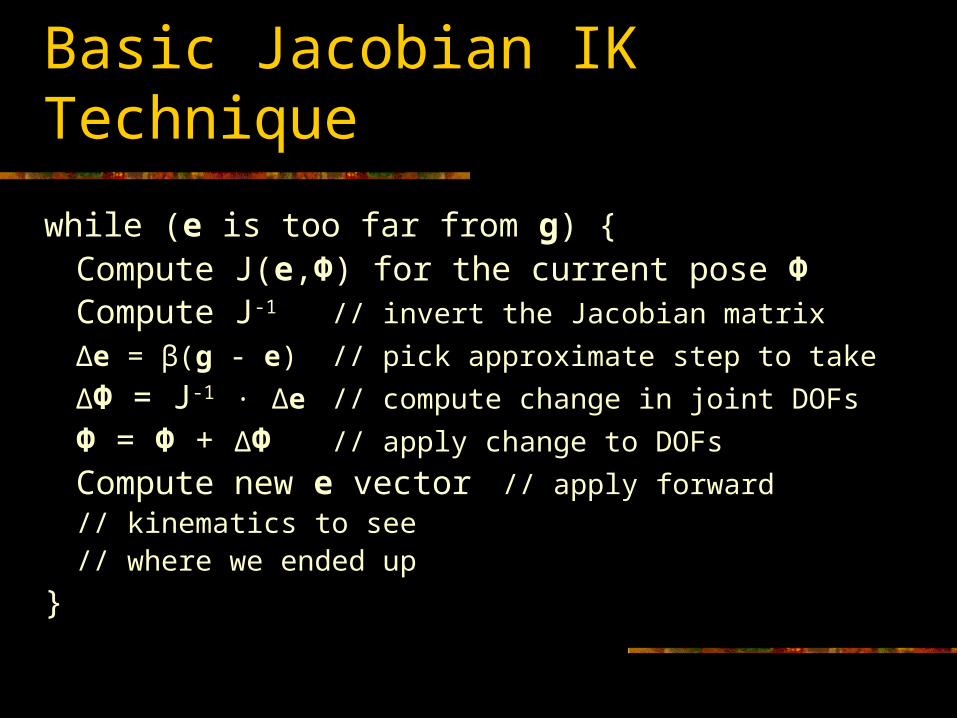
Basic Jacobian IK Technique

while (e is too far from g) {Compute J(e,Φ) for the current pose ΦCompute J-1 // invert the Jacobian matrix

Δe = β(g - e) // pick approximate step to take

ΔΦ = J-1 · Δe // compute change in joint DOFs

Φ = Φ + ΔΦ // apply change to DOFs

Compute new e vector // apply forward// kinematics to see// where we ended up

}

Computing the Jacobian

Computing the Jacobian Matrix

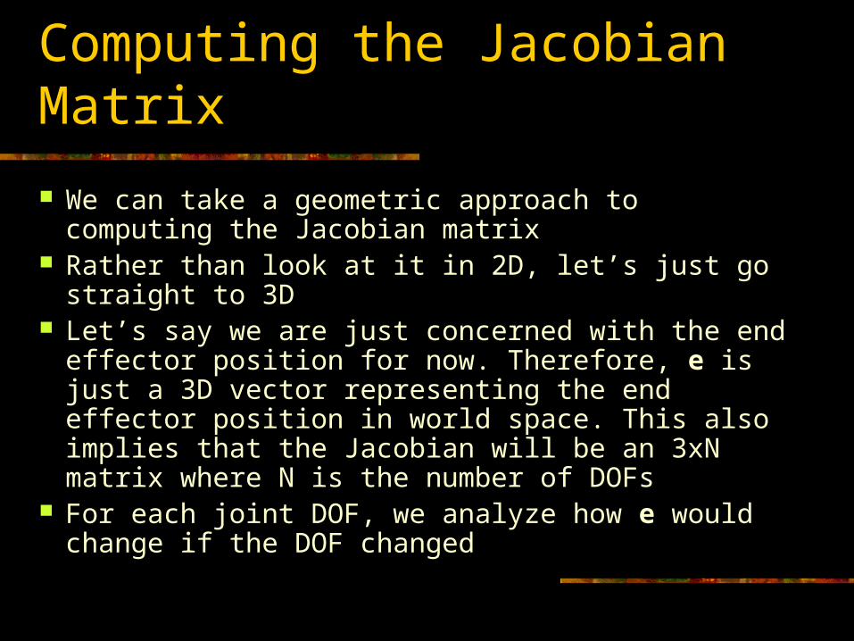
We can take a geometric approach to computing the Jacobian matrix

Rather than look at it in 2D, let’s just go straight to 3D

Let’s say we are just concerned with the end effector position for now. Therefore, e is just a 3D vector representing the end effector position in world space. This also implies that the Jacobian will be an 3xN matrix where N is the number of DOFs

For each joint DOF, we analyze how e would change if the DOF changed

1-DOF Rotational Joints

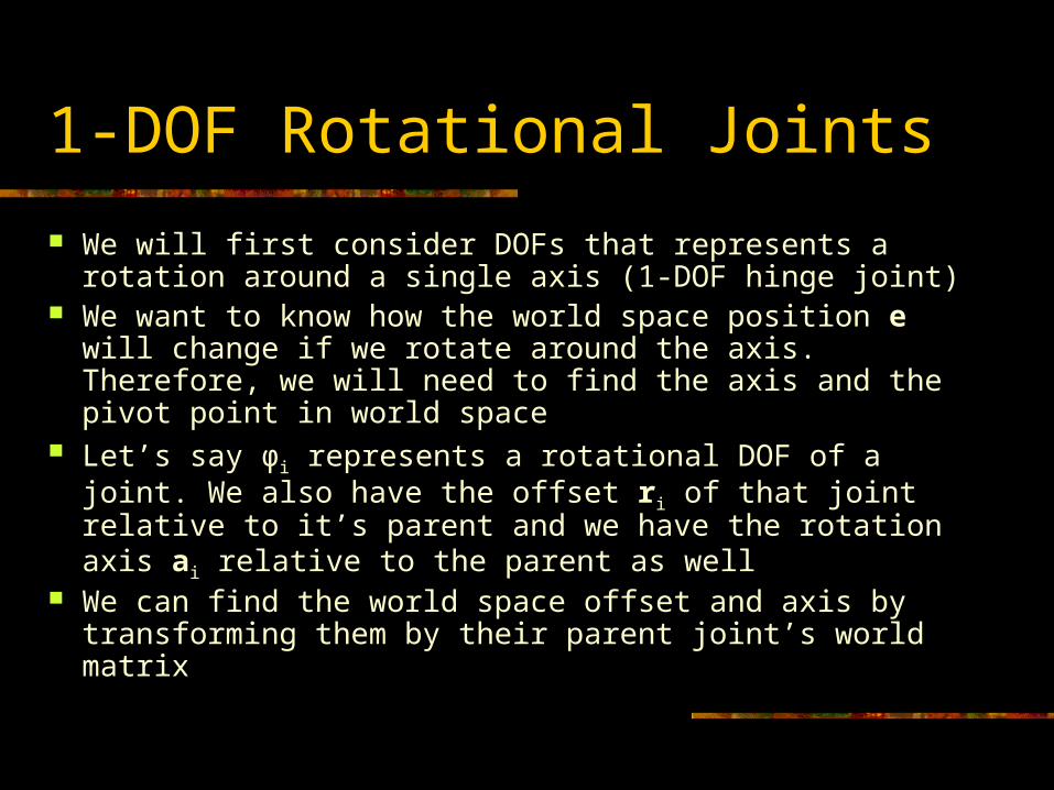
We will first consider DOFs that represents a rotation around a single axis (1-DOF hinge joint)

We want to know how the world space position e will change if we rotate around the axis. Therefore, we will need to find the axis and the pivot point in world space

Let’s say φi represents a rotational DOF of a joint. We also have the offset ri of that joint relative to it’s parent and we have the rotation axis ai relative to the parent as well

We can find the world space offset and axis by transforming them by their parent joint’s world matrix

1-DOF Rotational Joints

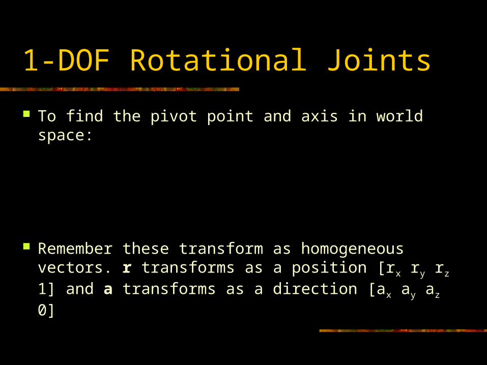
To find the pivot point and axis in world space:

Remember these transform as homogeneous vectors. r transforms as a position [rx ry rz 1] and a transforms as a direction [ax ay az 0]

parentiii

parentiii

Wrr

Waa

Rotational DOFs

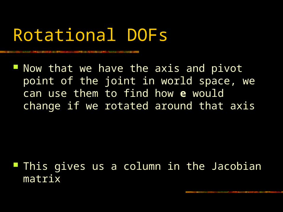
Now that we have the axis and pivot point of the joint in world space, we can use them to find how e would change if we rotated around that axis

This gives us a column in the Jacobian matrix

iii

reae

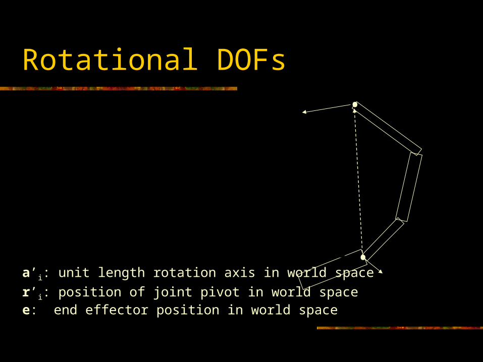
Rotational DOFs

a’i: unit length rotation axis in world space

r’i: position of joint pivot in world spacee: end effector position in world space

iii

reae

•

•i

e

ia

e

ire

ir

3-DOF Rotational Joints

For a 2-DOF or 3-DOF joint, it is actually a little trickier to get the world space axis

Consider how we would find the world space x-axis of a 3-DOF ball joint

Not only do we need to consider the parent’s world matrix, but we need to include the rotation around the next two axes (y and z-axis) as well

This is because those following rotations will rotate the first axis itself

3-DOF Rotational Joints

For example, assuming we have a 3-DOF ball joint that rotates in XYZ order:

Where Ry(θy) and Rz(θz) are y and z rotation matrices

parenti

parentzzi

parentzzyyi

Wa

WRa

WRRa

0100

0010

0001

:

:

:

dofz

dofy

dofx

3-DOF Rotational Joints

Remember that a 3-DOF XYZ ball joint’s local matrix will look something like this:

Where Rx(θx), Ry(θy), and Rz(θz) are x, y, and z rotation matrices, and T(r) is a translation by the (constant) joint offset

So it’s world matrix looks like this:

rTRRRL zzyyxxzyx ,,

parentzzyyxx WrTRRRW

3-DOF Rotational Joints

Once we have each axis in world space, each one will get a column in the Jacobian matrix

At this point, it is essentially handled as three 1-DOF joints, so we can use the same formula for computing the derivative as we did earlier:

We repeat this for each of the three axes

iii

reae

Quaternion Joints

What about a quaternion joint? How do we incorporate them into our IK formulation?

We will assume that a quaternion joint is capable of rotating around any axis

However, since we are trying to find a way to move e towards g, we should pick the best possible axis for achieving this

ii

iii rgre

rgrea

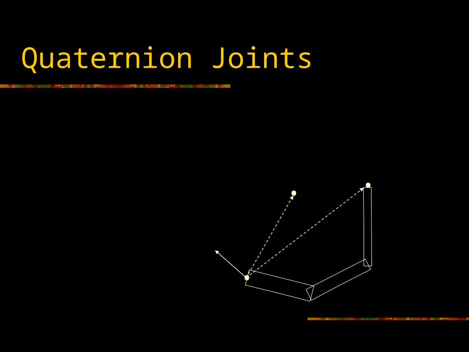
Quaternion Joints

ii

iii rgre

rgrea

•

• •e

irg ire

iria

g

Quaternion Joints

We compute ai’ directly in world space, so we don’t need to transform it

Now that we have ai’, we can just compute the derivative the same way we would do with any other rotational axis

We must remember what axis we use, so that later, when we’ve computed Δφi, we know how to update the quaternion

iii

reae

Translational DOFs

For translational DOFs, we start in the same way, namely by finding the translation axis in world space

If we had a prismatic joint (1-DOF translation) that could translate along an arbitrary axis ai defined in the parent’s space, we can use:

parentiii Waa

Translational DOFs

For a more general 3-DOF translational joint that just translates along the local x, y, and z-axes, we don’t need to do the same thing that we did for rotation

The reason is that for translations, a change in one axis doesn’t affect the other axes at all, so we can just use the same formula and plug in the x, y, and z axes [1 0 0 0], [0 1 0 0], [0 0 1 0] to get the 3 world space axes

Note: this will just return the a, b, and c axes of the parent’s world space matrix, and so we don’t actually have to compute them!

Translational DOFs

As with rotation, each translational DOF is still treated separately and gets its own column in the Jacobian matrix

A change in the DOF value results in a simple translation along the world space axis, making the computation trivial:

ii

ae

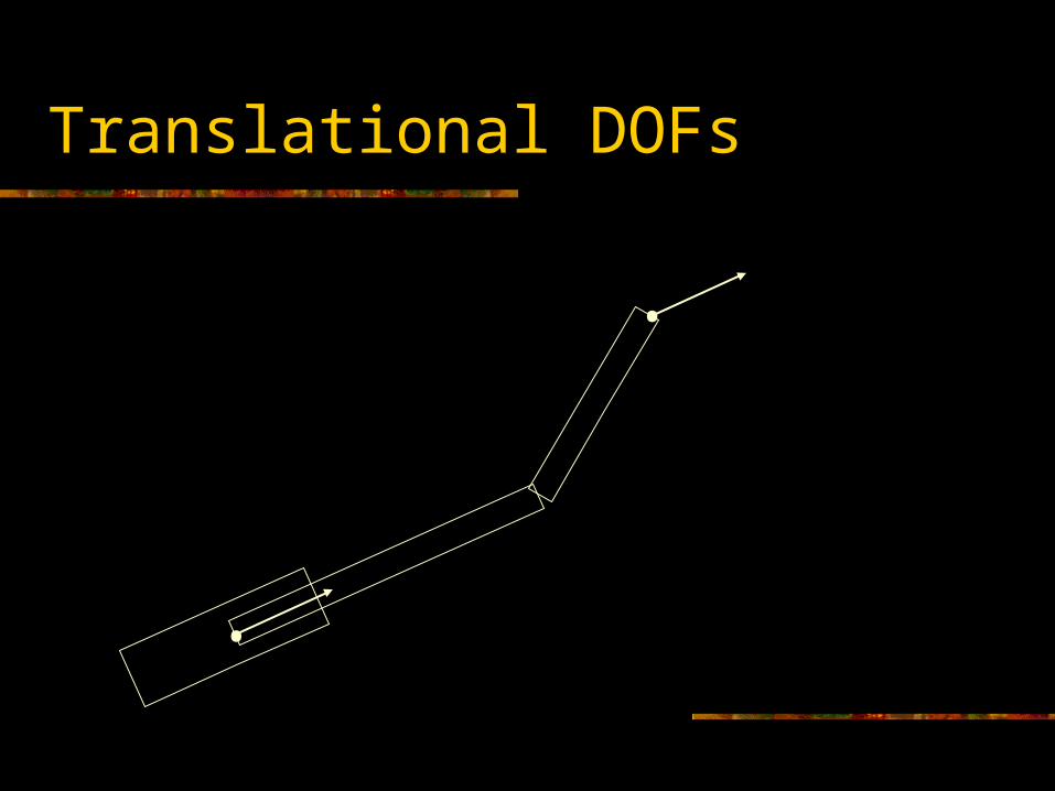
Translational DOFs

ia

ie

•

•

Building the Jacobian

To build the entire Jacobian matrix, we just loop through each DOF and compute a corresponding column in the matrix

If we wanted, we could use more elaborate joint types (scaling, translation along a path, shearing…) and still compute an appropriate derivative

If absolutely necessary, we could always resort to computing a numerical approximation to the derivative

Units & Scaling

What about units? Rotational DOFs use radians and translational

DOFs use meters (or some other measure of distance)

How can we combine their derivatives into the same matrix?

Well, it’s really a bit of a hack, but we just combine them anyway

If desired, we can scale any column to adjust how much the IK will favor using that DOF

Units & Scaling

For example, we could scale all rotations by some constant that causes the IK to behave how we would like

Also, we could use this as an additional way to get control over the behavior of the IK

We can store an additional parameter for each DOF that defines how ‘stiff’ it should behave

If we scale the derivative larger (but preserve direction), the solution will compensate with a smaller value for Δφi, therefore making it act stiff

There are several proposed methods for automatically setting the stiffness to a reasonable default value. They generally work based on some function of the length of the actual bone. The Welman paper talks about this.

End Effector Orientation

End Effector Orientation

We’ve examined how to form the columns of a Jacobian matrix for a position end effector with 3 DOFs

How do we incorporate orientation of the end effector?

We will add more DOFs to the end effector vector e Which method should we use to represent the

orientation? (Euler angles? Quaternions?…) Actually, a popular method is to use the 3 DOF

scaled axis representation!

Scaled Rotation Axis

We learned that any orientation can be represented as a single rotation around some axis

Therefore, we can store an orientation as an 3D vector The direction of the vector is the rotation axis The length of the vector is the angle to rotate in radians

This method has some properties that work well with the Jacobian approach Continuous and consistent No redundancy or extra constraints It’s also a nice method to store incremental changes in

rotation

6-DOF End Effector

If we are concerned about both the position and orientation of the end effector, then our e vector should contain 6 numbers

But remember, we don’t actually need the e vector, we really just need the Δe vector

To generate Δe, we compare the current end effector position/orientation (matrix E) to the goal position/orientation (matrix G)

The first 3 components of Δe represent the desired change in position: β(G.d - E.d)

The next 3 represent a desired change in orientation, which we will express as a scaled axis vector

Desired Change in Orientation

We want to choose a rotation axis that rotates E in to G We can compute this using some quaternions:

M=E-1·Gq.FromMatrix(M);

This gives us a quaternion that represents a rotation from E to G

To extract out the rotation axis and angle, we just remember that:

We can then scale the final axis by β

2sin

2sin

2sin

2cos

zyx aaaq

End Effector

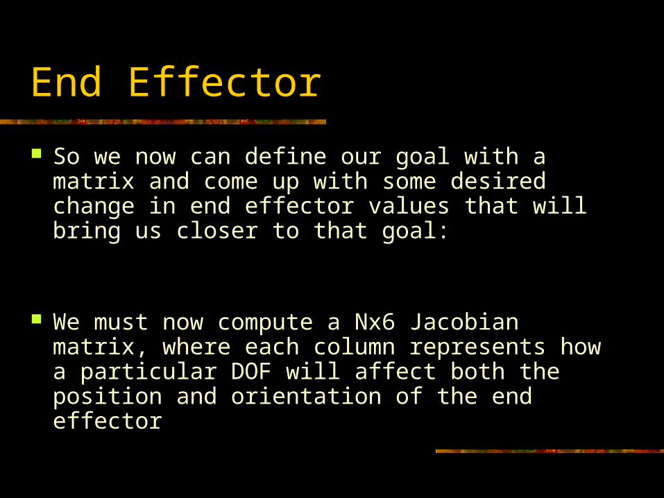
So we now can define our goal with a matrix and come up with some desired change in end effector values that will bring us closer to that goal:

We must now compute a Nx6 Jacobian matrix, where each column represents how a particular DOF will affect both the position and orientation of the end effector

Tzyxzyx ttt e

Rotational DOFs

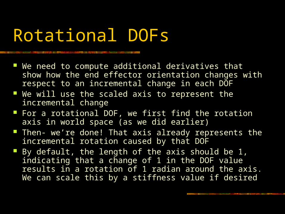
We need to compute additional derivatives that show how the end effector orientation changes with respect to an incremental change in each DOF

We will use the scaled axis to represent the incremental change

For a rotational DOF, we first find the rotation axis in world space (as we did earlier)

Then- we’re done! That axis already represents the incremental rotation caused by that DOF

By default, the length of the axis should be 1, indicating that a change of 1 in the DOF value results in a rotation of 1 radian around the axis. We can scale this by a stiffness value if desired

Rotational DOFs

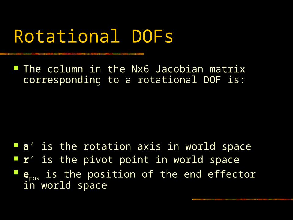
The column in the Nx6 Jacobian matrix corresponding to a rotational DOF is:

a’ is the rotation axis in world space r’ is the pivot point in world space epos is the position of the end effector in world space

T

i

Tiposi

ii

a

reaeJ

Translational DOFs

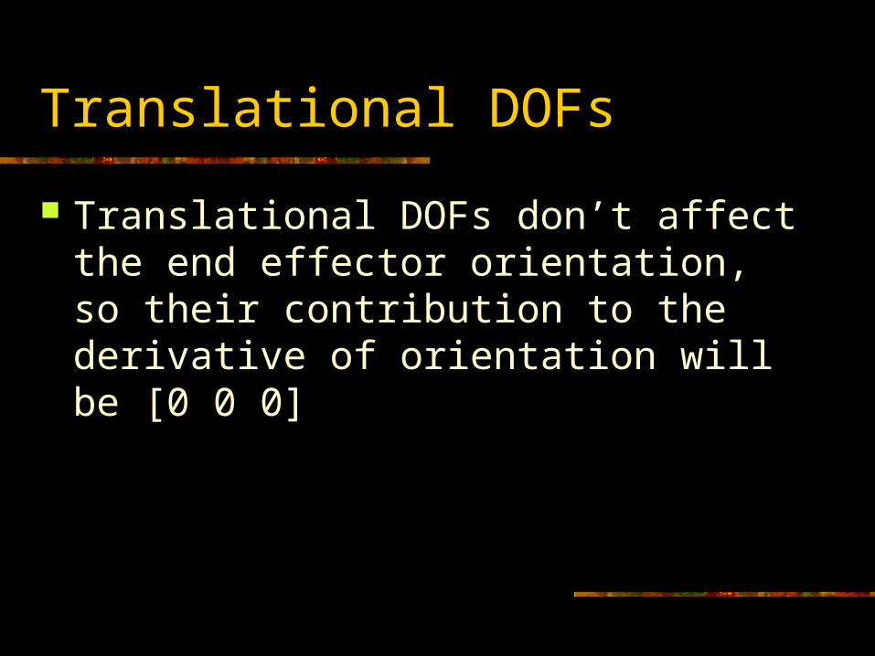
Translational DOFs don’t affect the end effector orientation, so their contribution to the derivative of orientation will be [0 0 0]

0

0

0

Ti

ii

a

eJ

Inverting the Jacobian Matrix

Inverting the Jacobian

If the Jacobian is square (number of joint DOFs equals the number of DOFs in the end effector), then we might be able to invert the matrix

Most likely, it won’t be square, and even if it is, it’s definitely possible that it will be singular and non-invertable

Even if it is invertable, as the pose vector changes, the properties of the matrix will change and may become singular or near-singular in certain configurations

The bottom line is that just relying on inverting the matrix is not going to work

Underconstrained Systems

If the system has more degrees of freedom in the joints than in the end effector, then it is likely that there will be a continuum of redundant solutions (i.e., an infinite number of solutions)

In this situation, it is said to be underconstrained or redundant

These should still be solvable, and might not even be too hard to find a solution, but it may be tricky to find a ‘best’ solution

Overconstrained Systems

If there are more degrees of freedom in the end effector than in the joints, then the system is said to be overconstrained, and it is likely that there will not be any possible solution

In these situations, we might still want to get as close as possible

However, in practice, overconstrained systems are not as common, as they are not a very useful way to build an animal or robot (they might still show up in some special cases though)

Well-Constrained Systems

If the number of DOFs in the end effector equals the number of DOFs in the joints, the system could be well constrained and invertable

In practice, this will require the joints to be arranged in a way so their axes are not redundant

This property may vary as the pose changes, and even well-constrained systems may have trouble

Pseudo-Inverse

If we have a non-square matrix arising from an overconstrained or underconstrained system, we can try using the pseudoinverse:

J*=(JTJ)-1JT

This is a method for finding a matrix that effectively inverts a non-square matrix

Degenerate Cases

•

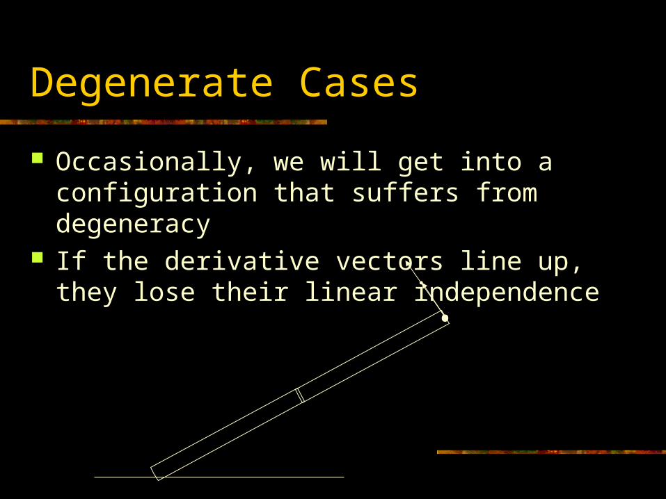
Occasionally, we will get into a configuration that suffers from degeneracy

If the derivative vectors line up, they lose their linear independence

Single Value Decomposition

The SVD is an algorithm that decomposes a matrix into a form whose properties can be analyzed easily

It allows us to identify when the matrix is singular, near singular, or well formed

It also tells us about what regions of the multidimensional space are not adequately covered in the singular or near singular configurations

The bottom line is that it is a more sophisticated, but expensive technique that can be useful both for analyzing the matrix and inverting it

Jacobian Transpose

Another technique is to simply take the transpose of the Jacobian matrix!

Surprisingly, this technique actually works pretty well It is much faster than computing the inverse or

pseudo-inverse Also, it has the effect of localizing the computations.

To compute Δφi for joint i, we compute the column in the Jacobian matrix Ji as before, and then just use:

Δφi = JiT · Δe

Jacobian Transpose

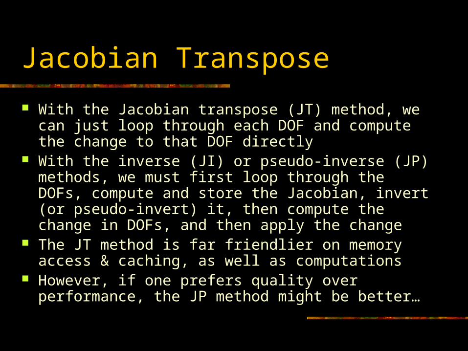
With the Jacobian transpose (JT) method, we can just loop through each DOF and compute the change to that DOF directly

With the inverse (JI) or pseudo-inverse (JP) methods, we must first loop through the DOFs, compute and store the Jacobian, invert (or pseudo-invert) it, then compute the change in DOFs, and then apply the change

The JT method is far friendlier on memory access & caching, as well as computations

However, if one prefers quality over performance, the JP method might be better…

Iterating to the Solution

Iteration

Whether we use the JI, JP, or JT method, we must address the issue of iteration towards the solution

We should consider how to choose an appropriate step size β and how to decide when the iteration should stop

When to Stop

There are three main stopping conditions we should account for Finding a successful solution (or close enough) Getting stuck in a condition where we can’t improve

(local minimum) Taking too long (for interactive systems)

All three of these are fairly easy to identify by monitoring the progress of Φ

These rules are just coded into the while() statement for the controlling loop

Finding a Successful Solution

We really just want to get close enough within some tolerance

If we’re not in a big hurry, we can just iterate until we get within some floating point error range

Alternately, we could choose to stop when we get within some tolerance measurable in pixels

For example, we could position an end effector to 0.1 pixel accuracy

This gives us a scheme that should look good and automatically adapt to spend more time when we are looking at the end effector up close (level-of-detail)

Local Minima

If we get stuck in a local minimum, we have several options Don’t worry about it and just accept it as the best we

can do Switch to a different algorithm (CCD…) Randomize the pose vector slightly (or a lot) and try

again Send an error to whatever is controlling the end effector

and tell it to try something else Basically, there are few options that are truly appealing, as

they are likely to cause either an error in the solution or a possible discontinuity in the motion

Taking Too Long

In a time critical situation, we might just limit the iteration to a maximum number of steps

Alternately, we could use internal timers to limit it to an actual time in seconds

Iteration Stepping

Step size Stability Performance

Other IK Issues

Joint Limits

A simple and reasonably effective way to handle joint limits is to simply clamp the pose vector as a final step in each iteration

One can’t compute a proper derivative at the limits, as the function is effectively discontinuous at the boundary

The derivative going towards the limit will be 0, but coming away from the limit will be non-zero. This leads to an inequality condition, which can’t be handled in a continuous manner

We could just choose whether to set the derivative to 0 or non-zero based on a reasonable guess as to which way the joint would go. This is easy in the JT method, but can potentially cause trouble in JI or JP

Higher Order Approximation

The first derivative gives us a linear approximation to the function

We can also take higher order derivatives and construct higher order approximations to the function

This is analogous to approximating a function with a Taylor series

Repeatability

If a given goal vector g always generates the same pose vector Φ, then the system is said to be repeatable

This is not likely to be the case for redundant systems unless we specifically try to enforce it

If we always compute the new pose by starting from the last pose, the system will probably not be repeatable

If, however, we always reset it to a ‘comfortable’ default pose, then the solution should be repeatable

One potential problem with this approach however is that it may introduce sharp discontinuities in the solution

Multiple End Effectors

Remember, that the Jacobian matrix relates each DOF in the skeleton to each scalar value in the e vector

The components of the matrix are based on quantities that are all expressed in world space, and the matrix itself does not contain any actual information about the connectivity of the skeleton

Therefore, we extend the IK approach to handle tree structures and multiple end effectors without much difficulty

We simply add more DOFs to the end effector vector to represent the other quantities that we want to constrain

However, the issue of scaling the derivatives becomes more important as more joints are considered

Multiple Chains

Another approach to handling tree structures and multiple end effectors is to simply treat it as several individual chains

This works for characters often, as we can animate the body with a forward kinematic approach, and then animate each limb with IK by positioning the hand/foot as the end effector goal

This can be faster and simpler, and actually offer a nicer way to control the character

Geometric Constraints

One can also add more abstract geometric constraints to the system Constrain distances, angles within the skeleton Prevent bones from intersecting each other or the

environment Apply different weights to the constraints to signify their

importance Have additional controls that try to maximize the

‘comfort’ of a solution Etc.

Welman talks about this in section 5

Other IK Techniques

Cyclic Coordinate Descent This technique is more of a trigonometric approach and is more

heuristic. It does, however, tend to converge in fewer iterations than the Jacobian methods, even though each iteration is a bit more expensive. Welman talks about this method in section 4.2

Analytical Methods For simple chains, one can directly invert the forward kinematic

equations to obtain an exact solution. This method can be very fast, very predictable, and precisely controllable. With some finesse, one can even formulate good analytical solvers for more complex chains with multiple DOFs and redundancy

Other Numerical Methods There are lots of other general purpose numerical methods for

solving problems that can be cast into f(x)=g format

Jacobian Method as a Black Box

The Jacobian methods were not invented for solving IK. They are a far more general purpose technique for solving systems of non-linear equations

The Jacobian solver itself is a black box that is designed to solve systems that can be expressed as f(x)=g ( e(Φ)=g )

All we need is a method of evaluating f and J for a given value of x to plug it into the solver

If we design it this way, we could conceivably swap in different numerical solvers (JI, JP, JT, damped least-squares, conjugate gradient…)