Inverse kinematics for optimal tool

orientation control in 5-axis CNC machining

Rida T. Farouki,1 Chang Yong Han,2 and Shiqiao Li1

1 Department of Mechanical and Aerospace Engineering,

University of California, Davis, CA 95616, USA

2 Department of Applied Mathematics, Kyung Hee University,Yongin–si, Gyeonggi–do 446–701, SOUTH KOREA

Abstract

The problem of determining the inputs to the rotary axes of a 5–axisCNC machine is addressed, such that relative variations of orientationbetween the tool axis and surface normal are minimized subject to theconstraint of maintaining a constant cutting speed with a ball-end tool.In the context of an orientable–spindle machine, the results of a priorstudy are directly applicable to the solution of this inverse–kinematicsproblem. However, since they are expressed in terms of the integral ofthe geodesic curvature, a discrete time–step solution is proposed thatyields accurate rotary–axis increments at high sampling frequencies.For an orientable–table machine, a closed–form solution that specifiesthe rotary–axis positions as functions of the surface normal variationalong the toolpath is possible. In this context, however, the feasibilityof a solution is dependent upon the surface normal along the toolpathsatisfying certain orientational constraints. These inverse–kinematicssolutions facilitate accurate and efficient 5–axis machining of free–formsurfaces without “unnecessary” actuation of the machine rotary axes.

keywords: 5–axis CNC machining; tool orientation; inverse kinematics;ball–end tool; orientable–spindle machine; orientable–table machine.

e–mail: farouki@ucdavis.edu, cyhan@khu.ac.kr, shqli@ucdavis.edu

1 Introduction

A 5–axis CNC machine incorporates three translational and two rotationaldegrees of freedom to maintain the desired relative position and orientation ofthe cutting tool and workpiece during the execution of a part program. Therotary axes of 5–axis machines permit more intricate part shapes to be cut,without re–fixturing of the workpiece, than with 3–axis machines. However,the development of part programs for accurate and efficient 5–axis machiningof free–form surfaces is a challenging problem [2, 8, 10, 11, 12, 17, 18, 22, 23]for which fully–automated solutions have remained elusive — see Section 2of [6] for a more comprehensive review of the literature.

The problem of orienting the tool axis a with respect to the surface normaln along a smooth curve on the surface, so as to minimize orientational changeswhile satisfying (for a given angle ψ) the fixed cutting speed condition a ·n =cosψ, was considered in [6]. It was observed that, in the workpiece (x, y, z)coordinate system, the solution to this problem corresponds to specifying theorientation of the tangent–plane component at = a− cosψ n of a relative tothe Darboux frame by an angle φ specified (modulo a constant) by minus theintegral of the geodesic curvature with respect to arc length along the curve.Equivalently, at has no instantaneous rotation about the surface normal.

The optimal tool orientation strategy proposed in [6] is directly applicableto an orientable–spindle machine, in which the workpiece maintains a fixedorientation, and the rotary axes control the tool orientation. In an orientable–

table machine, on the other hand, the tool maintains a fixed orientation, andthe rotary axes control the orientation of the table upon which the workpieceis mounted. For both types of machine, the inverse kinematics problem forthe rotational axes must be solved, i.e., within each sampling interval of thedigital controller, the angular positions of those axes must be determined soas to maintain the desired relative tool/workpiece orientation.

In general, finite spatial rotations about distinct axes do not commute —i.e., the end result depends on the order in which the rotations are performed.However, for the specific configurations of orientable–spindle and orientable–table machines — with one stationary rotation axis, and the second rotationaxis mounted upon (and moving with) it — finite axis rotations do commute,so their order is unimportant. The transformation of a vector specified withthe machine axes in “home” position to a general machine orientation canthus be described by a single rotation matrix that depends on two angularparameters, namely, the rotary–axis inputs. This fact facilitates a solution of

2

the inverse–kinematics problem, for both orientable–spindle and orientable–table machines, so as to achieve the desired relative orientation of a and nat each point along a prescribed toolpath on a smooth surface.

The remainder of this paper is organized as follows. The basic problem ofoptimal tool/workpiece orientation control, under the constraint of a constantcutting speed using a ball–end tool, is introduced in Section 2 in the contextof both orientable–spindle and orientable–table machines. Some backgrounddifferential geometry of paths on smooth surfaces is then briefly reviewed inSection 3. In Section 4, the canonical configurations of the rotational axes onorientable–spindle and orientable–table machines are described, and a matrixformulation for general spatial rotations is presented. Section 5 addresses theinverse–kinematics solution for orientable–spindle machines, using the resultsfrom [6]. Since the solution involves the integral of the geodesic curvaturewith respect to arc length along the toolpath, which does not generally admita closed–form reduction, a discrete time–step method is proposed that yieldsaccurate results for sufficiently high sampling rates. The inverse kinematicsof orientable–table machines, considered in Section 6, is simpler and admitsa general closed–form solution for the rotary–axis inputs, expressed only interms of the surface normal variation along the toolpath. Finally, Section 7summarizes the main results of the present study, and identifies some openproblems that warrant further investigation.

2 Optimal tool/workpiece orientation

The problem addressed herein concerns the specification of tool orientationin 5–axis machining of free–form shapes with a spherical or “ball–end” toolof given radius R. Such a tool permits gouge–free machining of any surfacewith smallest concave principal radius of curvature not less than R. If thetool has angular speed n rpm and 0 < ψ < 1

2π is the angle between the tool

axis a and the surface normal n at the contact point, the cutting speed is

vc =2πn

60R sinψ .

Thus, to maintain a constant cutting speed, the polar angle of a with respectto n (or n with respect to a) must be equal to ψ, but the azimuthal angle ofa with respect to n (or n with respect to a) remains indeterminate.

The methodology proposed in [6] achieves “optimal” satisfaction of theconstant cutting–speed condition, by eliminating any relative motion between

3

a and n that is superfluous to its maintenance. Choosing the surface normaln as a reference, as in [6], means that the component of a parallel to n isa‖ = cosψ n, while the perpendicular component a⊥ = a−a‖ should exhibitno instaneous rotation about n. This interpretation is directly applicable tothe orientable–spindle machine context. In the context of an orientable–tablemachine, however, it is more convenient to choose the (stationary) tool axis aas a reference: we then require the component of the surface normal n parallelto a to be n‖ = cosψ a, while the perpendicular component n⊥ = n − n‖

should exhibit no instaneous rotation about a.For the orientable–spindle machine, it was shown in [6] that the desired

motion is realized if a is specified as a fixed vector in an orthonormal frame(n,v,w) that is rotation–minimizing1 with respect to n — i.e., its angularvelocity ω must satisfy ω ·n ≡ 0. The tangent–plane vectors of such a framehave an angular orientation φ, relative to the tangent–plane vectors of theDarboux frame, specified (modulo a constant) by minus the integral of thegeodesic curvature with respect to the toolpath arc length — see Section 3.As described in Section 5, this result facilitates determination of the rotary–axis inputs for the orientable–spindle machine in terms of φ. However, sincethe integral defining φ does not in general admit analytic reduction, a discretetime–step scheme for the rotary–axis inputs is also developed in Section 5,appropriate to controllers with sufficiently high sampling frequencies.

For the orientable–table machine, the inverse–kinematics formulation isin some respects simpler than for the orientable–spindle machine, since thetool axis vector is stationary and only the workpiece orientation is varied toachieve the desired relative behavior of a and n. In fact, when n‖ = cosψ aand n⊥ = n−n‖ has no instantaneous rotation about a for a fixed vector a, itis clear that the workpiece orientation must vary such as to make the surfacenormal n at each point of the toolpath coincide with some fixed vector n0.The integral φ is not required in this context, and a closed–form solution forthe rotary–axis inputs is possible, as described in Section 6.

3 Geometry of surface toolpaths

Consider a curve r(ξ) = s(u(ξ), v(ξ)) on a smooth surface s(u, v) defined byexpressing the surface parameters u, v as functions of a path parameter ξ.

1Rotation–minimizing frames have been studied [1, 3, 4, 5, 9, 14, 21] in the context ofapplications to computer animation, spatial motion design, and swept surface construction.

4

Differentiating by the chain rule gives

r′(ξ) = u′(ξ) su(u(ξ), v(ξ)) + v′(ξ) sv(u(ξ), v(ξ))

where su, sv are the partial derivatives of s(u, v). The parametric speed ofr(ξ) — i.e., the rate of change of arc length s with the parameter ξ — is

σ =ds

dξ= | r′ | = | u′ su + v′ sv | . (1)

Assuming that su × sv 6= 0 everywhere, the unit surface normal is defined ateach point by

n =su × sv

| su × sv |. (2)

The Darboux frame (n, t,u) along the curve r(ξ) = s(u(ξ), v(ξ)) is a set ofthree orthonormal vectors, where the surface normal n is defined by (2), thetangent to the curve r(ξ) is specified as

t =r′

| r′ |=

u′ su + v′ sv

| u′ su + v′ sv |, (3)

and the tangent normal u is a vector in the surface tangent plane orthogonalto t, defined by

u = n × t . (4)

The variation of the Darboux frame is described by the equations

n′

t′

u′

= σ

0 −κn τgκn 0 κg

−τg −κg 0

ntu

, (5)

where the quantities

κn =n · t′

σ, κg =

u · t′

σ, τg =

u · n′

σ(6)

define the normal curvature, geodesic curvature, and geodesic torsion [15, 20]along the path r(ξ) = s(u(ξ), v(ξ)). The relations (5) can be expressed as

n′ = σΩ × n , t′ = σΩ × t , u′ = σΩ × u ,

5

where the angular velocity Ω of the Darboux frame [15, 20] along r(ξ) is

Ω = κg n − τg t − κn u . (7)

In lieu of t and u, we introduce new basis vectors v and w for the surfacetangent plane, defined by

v = cosφ t + sinφ u , w = − sinφ t + cos φ u , (8)

with

φ = φ0 −

∫ ξ

0

κg σ dξ , (9)

where φ0 is an integration constant. With this choice, the derivatives

v′ = σ (κn cosφ− τg sin φ)n , w′ = −σ (κn sinφ+ τg cosφ)n (10)

of the tangent–plane vectors v, w are always parallel to the surface normaln. Equivalently, the orthonormal frame (n,v,w) is rotation–minimizing withrespect to n — i.e., if the variation of this frame is described by its angularvelocity ω such that

v′ = σω × v , w′ = σω ×w , n′ = σω × n

then ω · n ≡ 0, so v and w exhibit no instantaneous rotation about n.Since (v,w,n) is an orthonormal basis, v′ and w′ are parallel to n if and

only if v ·v′ = w ·v′ = 0 and v ·w′ = w ·w′ = 0. Now v ·v′ = w ·w′ = 0 is aconsequence of the fact that v and w are unit vectors. Also, differentiatingv ·w = 0 gives v′ ·w + v ·w′ = 0, and hence v′ ·w = 0 ⇔ v ·w′ = 0. Thus,either of the conditions

v′ · w = 0 or v · w′ = 0 (11)

suffices to ensure that the frame (n,v,w) is rotation–minimizing with respectto n. It is evident from (8) and (10) that these conditions are satisfied.

In [6] the tool axis vector a was specified in terms of the frame (n,v,w)and a fixed angle ψ, determined by the desired cutting speed, as

a = cosψ n + sinψ v . (12)

Note that the angular velocity ω of the frame (n,v,w) — and thus of the toolaxis vector a — is obtained by dropping the n component of the Darbouxframe angular velocity (7), i.e., it is just

ω = − τg t − κn u . (13)

6

4 Inverse kinematics for rotary axes

During each sampling interval of the servosystem, the real–time interpolatorfor the rotary axes of a 5–axis CNC machine must determine the incrementalaxis rotations necessary to maintain a prescribed orientation of the cuttingtool relative to the workpiece. Two canonical 5–axis machine configurations,the orientable–spindle machine and orientable–table machine, are consideredhere. The former employs a spindle of variable orientation and a workpiecetable of fixed orientation, while the latter has a fixed–orientation spindle anda workpiece table whose orientation can be varied. These are two of threebasic 5–axis machine configurations [13, 16, 19] — the third being a hybrid ofthe orientable–spindle and orientable–table forms, whose inverse kinematicscan be deduced by suitable adaptation of the methods described below.

The configurations of the rotary axes of orientable–spindle and orientable–table machines are analogous to those of an altazimuth mount for a telescopeor theodolite, with one fixed axis and a second axis that is mounted on thefirst and rotates with it, in the plane orthogonal to the first axis. Let (x, y, z)be a stationary coordinate system aligned with the machine translational axesand let (i, j,k) be associated unit vectors. The orientable–spindle machineincorporates rotary a and b axes, aligned with the x and y directions when themachine is in “home” position. The angular positions of these axes, relativeto home position, are denoted by α and β. The b rotary axis is attached tothe machine frame and always aligned with the y direction, but the a rotaryaxis is mounted on the b axis and moves with it. The instantaneous sense ofrotation associated with the a and b axes is thus defined by the unit vectors

ma = cosβ i − sin β k , mb = j . (14)

The range of feasible positions for the rotary axes on the orientable–spindlemachine are assumed to be α ∈ (−1

2π,+1

2π) and β ∈ (−1

2π,+1

2π).

The orientable–table machine employs rotary c and a axes, aligned withthe z and x directions in “home” position. The angular positions of theseaxes relative to home position are denoted by γ and α. The c axis is attachedto the machine frame and always aligned with the z direction, but the a axisis mounted on the c axis and moves with it. Thus, the instantaneous senseof rotation associated with the c and a axis is defined by the unit vectors

mc = k , ma = cos γ i + sin γ j . (15)

7

The feasible positions of the rotary axes on the orientable–table machine areassumed to be γ ∈ (−π,+π ] and α ∈ (−1

2π,+1

2π).

The basic configurations of orientable–spindle and orientable–table 5–axisCNC machines are illustrated in Figure 1. In general, the result of two finitespatial rotations about distinct axes depends on the order in which they areapplied. However, as shown in Sections 5 and 6 below, this problem does notarise with the specific rotary–axis configurations of an orientable–spindle ororientable–table machine — i.e., the current angular positions (α, β) or (γ, α)of the rotary axes uniquely determine the relative tool/workpiece orientation.

Figure 1: Standard configurations of the rotary axes on 5–axis CNC machines— an orientable–spindle machine (left) and orientable–table machine (right).For the former, the directions of the rotary axes that determine the spindleorientation are specified by (14). For the latter, the directions of the rotaryaxes that determine the workpiece table orientation are specified by (15).

The inverse kinematics problem, addressed by the rotary–axes real–timeinterpolator, amounts to determining the increments to the current rotary–axis orientations that are required during each sampling interval ∆t of theservosystem, in order to maintain a desired relative orientation of the tool andworkpiece. In some cases, it is possible to determine the rotary–axis inputsas continuous closed–form expressions in the path parameter ξ, that can besampled through increments ∆ξ determined by the feedrate (i.e., speed of the

8

tool along the path) and sampling interval ∆t. In other cases, a discrete time–step scheme may be used to determine the required axis angular increments.For typical 5–axis CNC machines, with sampling frequencies f of 1–10 kHz orhigher (and sampling intervals ∆t = 1/f = 0.001–0.0001 second or smaller),simple first–order methods furnish sufficient accuracy for practical use.

A rotation of a vector through angle θ about an axis specified by the unitvector m = (mx, my, mz) is defined by its product with an orthogonal matrix

M =

m11 m12 m13

m21 m22 m23

m31 m32 m33

(16)

whose elements are given [7] by

m11 = m2x + (1 −m2

x) cos θ ,

m12 = mxmy(1 − cos θ) −mz sin θ ,

m13 = mzmx(1 − cos θ) +my sin θ ,

m21 = mxmy(1 − cos θ) +mz sin θ ,

m22 = m2y + (1 −m2

y) cos θ ,

m23 = mymz(1 − cos θ) −mx sin θ ,

m31 = mzmx(1 − cos θ) −my sin θ ,

m32 = mymz(1 − cos θ) +mx sin θ ,

m33 = m2z + (1 −m2

z) cos θ . (17)

In the special case of rotations about the x, y, z axes, the instances Mx,My,Mz

of this matrix become

1 0 00 cos θ − sin θ0 sin θ cos θ

,

cos θ 0 sin θ0 1 0

− sin θ 0 cos θ

,

cos θ − sin θ 0sin θ cos θ 0

0 0 1

.

5 Orientable–spindle machine

Let α and β denote current orientations of the a and b rotary axes, relativeto the “home” position α = β = 0, corresponding to a spindle aligned withthe z–direction. Note that finite rotations about the a and b axes commute— i.e., their order is immaterial to the current spindle orientation. From (14)

9

and (16)–(17), a rotation by angle α (with β = 0) about a, followed with arotation by angle β (with α 6= 0) about b, corresponds to the matrix product

cosβ 0 sin β0 1 0

− sin β 0 cosβ

1 0 00 cosα − sinα0 sinα cosα

.

On the other hand, a rotation by angle β (with α = 0) about b, followed witha rotation by angle α (with β 6= 0) about a, corresponds to the product

cos2 β + sin2 β cosα sin β sinα sin β cosβ(cosα− 1)− sin β sinα cosα − cosβ sinα

sin β cos β(cosα− 1) cosβ sinα sin2 β + cos2 β cosα

cosβ 0 sin β0 1 0

− sin β 0 cosβ

.

Both products reduce to the same orthogonal matrix, namely

M =

cosβ sinα sin β cosα sin β0 cosα − sinα

− sin β sinα cosβ cosα cosβ

. (18)

This matrix may be regarded as mapping the tool axis vector in the homeposition, namely a = k, to a general orientation specified by

a = (ax, ay, az) = (cosα sin β,− sinα, cosα cosβ) . (19)

This expression defines the relation between the tool orientation vector a andthe axis rotation angles α, β.

The tool–orientation strategy proposed in [6] assumes a fixed workpieceorientation and a variable–orientation tool, and is thus directly applicable toorientable–spindle machines. The tool axis vector a specified by (8) and (12)can be written as

a = cosψ n + sinψ (cosφ t + sinφu) , (20)

where the dependence of the Darboux frame vectors (n, t,u) on ξ is given by(2)–(4), and the angle φ is specified as a function of ξ by (9). Note that theDarboux frame (n, t,u) — and hence the tool axis a — is specified in themachine (x, y, z) coordinates, since the workpiece orientation is invariant.

Noting that −12π < α, β < +1

2π, the rotary–axis angles may be expressed

from (19) in terms of the components ax(ξ), ay(ξ), az(ξ) of a(ξ) as

α(ξ) = − sin−1 ay(ξ) , β(ξ) = tan−1 ax(ξ)

az(ξ). (21)

10

Although this is an essentially closed–form solution for the rotary–axis inputs,it should be noted that the integral (9) does not admit an analytic reduction,except in trivial cases. In fact, the controller employs only a discrete samplingof the inputs (21), and sufficiently accurate sampled values can be obtainedusing first–order expansions in the increment ∆ξ of the path parameter.

Let ∆a denote the change in a incurred by an increment2 ∆ξ in the curveparameter ξ corresponding to one servosystem sampling interval ∆t. In thefollowing analysis, all quadratic and higher–order terms in ∆ξ are dropped,on the assumption that they are small compared to the linear terms. From(5), the variations in the Darboux frame vectors corresponding to a parameterincrement ∆ξ are

∆n = (τgu − κnt) σ∆ξ ,

∆t = (κnn + κgu) σ∆ξ ,

∆u = − (τgn + κgt) σ∆ξ ,

while the change in the angle (9) is

∆φ = −κg σ∆ξ .

Now for small ∆ξ, we have

cos(φ+ ∆φ) ≈ cosφ− ∆φ sinφ , sin(φ+ ∆φ) ≈ sin φ+ ∆φ cosφ ,

so the change ∆a = a(ξ + ∆ξ) − a(ξ) in (20) may be expressed as

∆a = cosψ∆n + sinψ [ cosφ∆t + sin φ∆u + (cosφu− sin φ t) ∆φ ] .

On substituting for ∆n,∆t,∆u and ∆φ this reduces to

∆a = [ sinψ(κn cos φ− τg sinφ)n− cosψ(κnt − τgu) ] σ∆ξ , (22)

and one can verify from (20) and (22) that

a · ∆a = 0 (23)

— as expected since a is, by definition, a unit vector.

2This increment is computed from the toolpath geometry and feedrate by the real–timeinterpolator for the translational machine axes.

11

The change (22) in the tool axis orientation (20) must be realized throughincremental rotations ∆α and ∆β of the spindle about the a and b axes, withdirections ma and mb specified by (14). For ∆α = O(∆ξ) and ∆β = O(∆ξ),we invoke the small–angle approximations (cos ∆α, sin ∆α) ≈ (1,∆α) and(cos ∆β, sin ∆β) ≈ (1,∆β) to define the incremental rotation matrices

Ma =

1 sin β∆α 0− sin β∆α 1 − cosβ∆α

0 cosβ∆α 1

, Mb =

1 0 ∆β0 1 0

−∆β 0 1

.

To first order in ∆ξ, the product M = Ma Mb = Mb Ma is then given by

M =

1 sin β∆α ∆β− sin β∆α 1 − cosβ∆α

−∆β cos β∆α 1

. (24)

The desired increments ∆α, ∆β are thus determined from the condition

M a = a + ∆a or (M − I) a = ∆a , (25)

where I is the 3 × 3 identity matrix, and thus

M − I =

0 sin β∆α ∆β− sin β∆α 0 − cos β∆α

−∆β cosβ∆α 0

. (26)

Writing a = (ax, ay, az) and ∆a = (∆ax,∆ay,∆az) the condition (25) is thenequivalent to the three scalar equations

sin β∆α ay + ∆β az = ∆ax ,

− sin β∆α ax − cos β∆α az = ∆ay ,

−∆β ax + cosβ∆α ay = ∆az ,

for ∆α and ∆β. The second equation yields

∆α = −∆ay

sin β ax + cosβ az

, (27)

and using ax∆ax+ay∆ay+az∆az = 0 from (23), the first and third equationsthen give

∆β =cosβ∆ax − sin β∆az

sin β ax + cosβ az

. (28)

12

Writing n = (nx, ny, nz), t = (tx, ty, tz), u = (ux, uy, uz) the components of∆a and a in (27)–(28) are obtained from (20) and (22) as

ax = cosψ nx + sinψ (cosφ tx + sinφ ux) ,

ay = cosψ ny + sinψ (cosφ ty + sin φ uy) ,

az = cosψ nz + sinψ (cosφ tz + sinφ uz) ,

∆ax = [ sinψ(κn cos φ− τg sinφ)nx − cosψ(κntx − τgux) ] σ∆ξ ,

∆ay = [ sinψ(κn cos φ− τg sinφ)ny − cosψ(κnty − τguy) ] σ∆ξ ,

∆az = [ sinψ(κn cos φ− τg sinφ)nz − cosψ(κntz − τguz) ] σ∆ξ .

It is understood, in expressions (27)–(28), that σ, n, t, u, κn, τg, and φ areall evaluated at the current ξ. Note that these expressions become singularif sin β ax + cos β az = 0. From (19) we observe that this corresponds to thecircumstance cosα = 0, i.e., α = ±1

2π and the tool is parallel to the y–axis.

The angular range of the a axis will typically be constrained by software orhardware limits to preclude this circumstance.

Starting with a given initial tool axis orientation, defined by (20) with aparticular choice for φ0 in (9), the rotary axis inputs for a path step ∆ξ aredetermined from (27) and (28), and the process is repeated after incrementingξ by ∆ξ. In this manner, the coordinated translational and rotational toolmotions that realize the scheme proposed in [6] are achieved.

Note that, if ∆a is computed from (25) using the matrix defined by(26) and (27)–(28) and the current β value, a + ∆a is no longer precisely aunit vector. Since we are only concerned with the tool orientation, it can beunitized at each step ∆ξ through division by |a+∆a|. However, it is perhapspreferable to compute a + ∆a by using α + ∆α, β + ∆β in (19), since it isthen guaranteed to be always of unit magnitude.

Example 1. To assess the accuracy of the incremental inverse–kinematicsscheme for the rotary axes of an orientable–spindle machine, we compare itsoutput with the known variation of a for a non–trivial example that admitsan exact closed–form solution [6]. Consider, on the torus defined for R > rand u, v ∈ [ 0, 2π ] by

s(u, v) = ((R + r cos v) cosu, (R+ r cos v) sin u, r sin v) , (29)

the path r(ξ) = s(u(ξ), v(ξ)) from r(0) = s(0, 0) = (R + r, 0, 0) to r(1) =s(1

2π, 1

2π) = (0, R, r) specified by

(u(ξ), v(ξ)) = (12πξ, 1

2πξ) (30)

13

for ξ ∈ [ 0, 1 ]. Figure 2 shows this path on the torus (29) with R = 2, r = 1and the surface normals

n =su × sv

| su × sv |= (cosu cos v, sin u cos v, sin v) (31)

along it. For the path (30), we have

r′(ξ) = u′(ξ) su(u(ξ), v(ξ)) + v′(ξ) sv(u(ξ), v(ξ))

and the parametric speed is

σ(ξ) = |r′(ξ)| = 1

2π η(ξ) , η(ξ) =

√

(R + r cos v(ξ))2 + r2 .

We henceforth omit the dependence u, v, σ, η on ξ. The tangent t = (tx, ty, tz) =r′/σ and tangent normal u = (ux, uy, uz) = n× t along (30) are defined by

η tx = − (R + r cos v) sinu− r cosu sin v ,

η ty = (R + r cos v) cosu− r sin u sin v ,

η tz = r cos v , (32)

η ux = r sin u− (R + r cos v) cosu sin v ,

η uy = − r cos u− (R + r cos v) sin u sin v ,

η uz = (R + r cos v) cos v , (33)

and from (6) the normal curvature, geodesic curvature, and geodesic torsioncan be expressed as

κn = −R cos v + r(1 + cos2 v)

(R + r cos v)2 + r2,

κg =sin v

√

(R + r cos v)2 + r2

[

1 +r2

(R + r cos v)2 + r2

]

,

τg =R

(R + r cos v)2 + r2.

It was shown in [6] that, for this example, the angle function (9) is given by

φ(ξ) = φ0 + cos 12πξ − 1 + tan−1

(

R

r+ cos 1

2πξ

)

− tan−1

(

R

r+ 1

)

. (34)

14

For the inclination angle ψ = 14π, the variation of the tool axis defined by

(20) and (34) along the path (30) is illustrated in Figure 2.To compute the axis angles α(ξ), β(ξ) and corresponding tool orientation

a(ξ) along the path (30) on the torus (29) incrementally using (27)–(28), theinitial orientation a(0) = (ax(0), ay(0), az(0)) is first determined from (9) and(20) with φ0 = 0. The initial axis angles α(0), β(0) are then determined byinvoking (19) to obtain

α(0) = sin−1 ay(0) , β(0) = tan−1 ax(0)

az(0).

In the present case α(0) = −42.1, β(0) = 72.5. With this initial condition,Figure 3 shows the variation of the axis angles α and β along the path onthe torus, computed using (27)–(28) with the increment ∆ξ = 0.001.

Figure 2: The path specified by (30) on the torus (29), with R = 2 and r = 1,showing the surface normal n (left) the tool axis a (right) along this path.

If a is the exact tool axis vector and a is the (unitized) tool axis vector,computed for any given parameter increment ∆ξ by the inverse–kinematicsscheme described above, we define for each ξ the non–negative error measure

ǫ = 1 − a · a , (35)

satisfying ǫ = 0 if and only if a = a. Figure 4 illustrates the variation of theerror measure (35) for parameter increments ∆ξ = 0.001 and ∆ξ = 0.0001.Note that the value ǫ = 10−6 corresponds to an angular deviation of ∼ 0.08,while ǫ = 10−8 corresponds to ∼ 0.008.

15

0.0 0.2 0.4 0.6 0.8 1.0–90o

–60o

–30o

0o

30o

60o

90o

ξ

axis

rot

atio

n an

gle

α

β

Figure 3: Variation of the rotary–axis angles α, β along the path (30) on thetorus (29), computed incrementally from (27)–(28), for an orientable–spindlemachine with initial spindle orientation defined by (9) and (20) with φ0 = 0.

0.0 0.2 0.4 0.6 0.8 1.010–10

10–8

10–6

10–4

10–2

100

ξ

ε∆ξ = 0.001

∆ξ = 0.0001

Figure 4: The error measure (35) for discrete computation of the tool axisalong the path (30) on the torus (29) for step sizes ∆ξ = 0.001 and 0.0001.

16

6 Orientable–table machine

The optimal tool orientation scheme developed in [6] implicitly assumes afixed workpiece orientation, and is directly applicable to orientable–spindlemachines. In the context of orientable–table machines, however, it requires are–interpretation. The method may be regarded as constraining the relative

orientation of the tool axis and surface normal at the tool contact point. In[6], the surface normal n is employed as a reference, and the tool axis a isdecomposed into components a‖ and a⊥ parallel and perpendicular to it. Theparallel component is just a‖ = cosψ n, while the perpendicular componenta⊥ is required to exhibit no instantaneous rotation about n.

In the context of an orientable–table machine, the tool axis a is fixed andthe workpiece (and with it the surface normal n) rotates about the c and aaxes. In this context, it is preferable to choose the tool axis a as a reference,and decompose the surface normal into components n‖ and n⊥ parallel andperpendicular to it. The desired relative motion of a and n is then achievedif n‖ = a cosψ and n⊥ exhibits no instantaneous rotation about a. Since a isaligned with the machine z–axis, this means that the actuation of the rotaryaxes must be such as to align the surface normal n at the tool contact pointwith a fixed unit vector n0 in the machine (x, y, z) coordinate system, as thecontact point traverses the given toolpath. Any departure from this conditionincurs a change of workpiece orientation that is superfluous to maintenanceof a fixed angle ψ between the tool axis a and surface normal n.

The fixed vector n0 can be expressed, for some chosen angle ζ , as

n0 = sinψ (cos ζ i + sin ζ j) + cosψ k .

For brevity, we henceforth assume ζ = 0 without loss of generality, so n0 =sinψ i + cosψ k. The surface must be initially oriented so that the normaln(0) at the toolpath start point r(0) = s(u(0), v(0)) is aligned with n0.

Let γ and α denote current orientations of the c and a rotary axes, relativeto the “home” position γ = α = 0, corresponding to a horizontal table whosesides are aligned with the x, y directions. From (15) and (16)–(17), a rotationby angle α (with γ = 0) about a, followed with a rotation by angle γ (withα 6= 0) about c, corresponds to the matrix product

cos γ − sin γ 0sin γ cos γ 0

0 0 1

1 0 00 cosα − sinα0 sinα cosα

.

17

On the other hand, a rotation by angle γ (with α = 0) about c, followed witha rotation by angle α (with γ 6= 0) about a, corresponds to the product

cos2 γ + sin2 γ cosα sin γ cos γ(1 − cosα) sin γ sinαsin γ cos γ(1 − cosα) sin2 γ + cos2 γ cosα − cos γ sinα

− sin γ sinα cos γ sinα cosα

cos γ − sin γ 0sin γ cos γ 0

0 0 1

.

Both products reduce to the same orthogonal matrix, namely

M =

cos γ − sin γ cosα sin γ sinαsin γ cos γ cosα − cos γ sinα

0 sinα cosα

. (36)

Hence, finite rotations about the c and a axes commute — i.e., their order isimmaterial to the current workpiece table orientation.

It is convenient to write n in terms of spherical polar coordinate angles(ϑ, ϕ) with 0 ≤ ϑ ≤ π and 0 ≤ ϕ ≤ 2π as

(nx, ny, nz) = (cos ϑ, sinϑ cosϕ, sinϑ sinϕ) , (37)

where cosϑ = nx, sin ϑ =√

n2y + n2

z and (cosϕ, sinϕ) = (ny, nz)/√

n2y + n2

z.The goal is to continuously orient the workpiece, by appropriate variations ofthe rotary–axis angles γ and α, so that the surface normal n at the contactpoint is always aligned with the fixed vector n0 = sinψ i + cosψ k.

Let γ(ξ) and α(ξ) be the angular positions of the c and a axes required toalign the surface normal n(ξ) = (nx(ξ), ny(ξ), nz(ξ)) at the point r(ξ) of thetoolpath with the fixed vector n0 = sinψ i + cosψ k — i.e., M(ξ)n(ξ) = n0,where M(ξ) is the matrix defined by substituting γ(ξ) and α(ξ) in (36). Thismatrix can be regarded as the solution of a system of first–order differentialequations (see the Appendix). Alternatively, one can solve for γ(ξ) and α(ξ)algebraically by noting that they must satisfy

cos γ(ξ)nx(ξ) − sin γ(ξ) (cosα(ξ)ny(ξ) − sinα(ξ)nz(ξ)) = sinψ ,

sin γ(ξ)nx(ξ) + cos γ(ξ) (cosα(ξ)ny(ξ) − sinα(ξ)nz(ξ)) = 0 ,

sinα(ξ)ny(ξ) + cosα(ξ)nz(ξ) = cosψ .

Substituting from (37), these equations can be re–formulated as

cos γ(ξ) cosϑ(ξ) − sin γ(ξ) sin ϑ(ξ) cos(α(ξ) + ϕ(ξ)) = sinψ ,

sin γ(ξ) cos ϑ(ξ) + cos γ(ξ) sin ϑ(ξ) cos(α(ξ) + ϕ(ξ)) = 0 ,

sinϑ(ξ) sin(α(ξ) + ϕ(ξ)) = cosψ . (38)

18

Adding the first and second equations, multiplied with cos γ(ξ) and sin γ(ξ)respectively, then gives

cos γ(ξ) =cos ϑ(ξ)

sinψ. (39)

Using this in conjunction with the second and third equations, we obtain

cos(α(ξ) + ϕ(ξ)) = −sinψ sin γ(ξ)

sinϑ(ξ), sin(α(ξ) + ϕ(ξ)) =

cosψ

sin ϑ(ξ). (40)

However, the orientable–table machine can achieve the desired motion onlyunder certain restrictions on the variation of the surface normal n along thegiven toolpath. Since 0 ≤ ϑ(ξ) ≤ π and 0 < ψ < 1

2π, equation (39) and the

second of equations (40) can only be satisfied when

| cosϑ(ξ)| ≤ sinψ and sinϑ(ξ) ≥ cosψ ,

and the first of equations (40) can then also be satisfied. These two conditionsare equivalent to the constraint

12π − ψ ≤ ϑ(ξ) ≤ 1

2π + ψ (41)

on the range of ϑ(ξ), i.e., the surface normal n(ξ) must lie outside a cone ofhalf–angle 1

2π − ψ about the positive/negative x–direction. The constraint

(41) must be satisfied at each point of the toolpath, to ensure that γ(ξ) andα(ξ) are properly defined by equations (39)–(40), and the machine is thuscapable of maintaining the desired relative tool/workpiece orientation.

In general, equation (39) determines two possible values γ1(ξ), γ2(ξ) in theinterval (−π,+π ] that differ only in sign. Since γ2(ξ) = − γ1(ξ), equations(40) give corresponding values α1(ξ), α2(ξ) = π−α1(ξ)− 2ϕ(ξ). Dependingon ϕ(ξ), however, they may not both lie in the allowed interval [−1

2π,+1

2π ]

for α(ξ). For example, when ϕ(ξ) = 0 and α1(ξ) ∈ [−12π,+1

2π ], then α2(ξ) ∈

[ 1

2π,+3

2π ] so γ1(ξ), α1(ξ) is the only feasible solution. On the other hand, if

ϕ(ξ) = 12π and α1(ξ) ∈ [−1

2π,+1

2π ], then α2(ξ) ∈ [−1

2π,+1

2π ] so γ1(ξ), α1(ξ)

and γ2(ξ), α2(ξ) are both feasible solutions that map n(ξ) onto n0.The motion should employ inputs γ(ξ) and α(ξ) that specify continuous

variations of the rotary–axis angles with the path parameter ξ, so as to alignthe surface normal n(ξ) with the fixed vector n0. To initialize the motion,the rotary axes must be set to the positions γ(0) and α(0) defined with ξ = 0in (39)–(40), to align the initial surface normal n(0) with n0.

19

In the case of an orientable–table machine, the rotary–axis inputs γ and αthat realize the optimal relative tool/workpiece orientation scheme proposedin [6] admit an essentially closed–form solution. Note that the function φ(ξ)defined by (9) is not required in the orientable–table context. In the case ofan orientable–spindle machine, φ(ξ) compensates for the non–zero angularvelocity component of the Darboux frame — which is employed to specify thetool orientation — in the surface normal direction. The inverse kinematics ofthe orientable–table machine is a simpler problem, since it is only concernedwith the orientation of the surface normal, relative to a fixed reference frame,along the toolpath. However, the existence of solutions is contingent uponconstraints on the variation of the surface normal along the toolpath.

Example 2. Consider the torus of Example 1 for the case of the orientable–table machine. Since condition (41) is not satisfied along the path (30) whenξ ∈ [ 0, 1 ] we use ξ ∈ [ 1

2, 3

2] instead. Comparing (31) and (37) yields

cosϑ(ξ) = cos2 12πξ , sinϑ(ξ) = sin 1

2πξ

√

1 + cos2 12πξ ,

cosϕ(ξ) =cos 1

2πξ

√

1 + cos2 12πξ

, sinϕ(ξ) =1

√

1 + cos2 12πξ

.

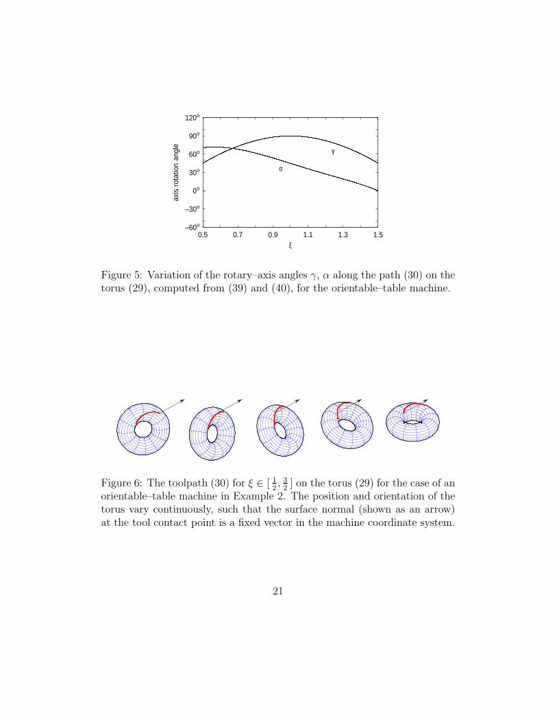
Then the rotary–axis inputs γ(ξ) and α(ξ) are defined by substituting theseexpressions into (39) and (40). In particular, we use the angle γ(ξ) satisfying(39) within the interval [ 0, π ]. Figure 5 illustrates the variations of the axisangles γ and α with the path parameter ξ computed in this manner.

The computation of the rotary–axis inputs is much simpler in this casethan for the orientable–spindle machine case described in Example 1, since itis not necessary to invoke the Darboux frame apparatus (5) and the function(9). Note, however, that the path (30) with ξ ∈ [ 0, 1 ] employed in Example 1is infeasible on the orientable–table machine, since the initial surface normaln(0) = (1, 0, 0) violates the condition (41). In the present context, a modifiedparameter interval ξ ∈ [ 1

2, 3

2] was necessary to ensure a feasible solution.

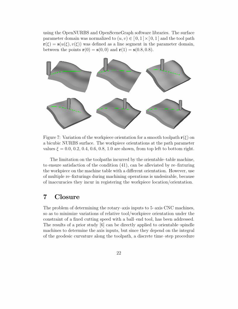
Figure 6 shows how the position/orientation of the torus is varied, usingthe toolpath r(ξ) and rotary–axis inputs γ(ξ) and α(ξ) computed above, soas to ensure that the surface normal n(ξ) at the contact point is transformedinto a fixed vector in the machine coordinate system.

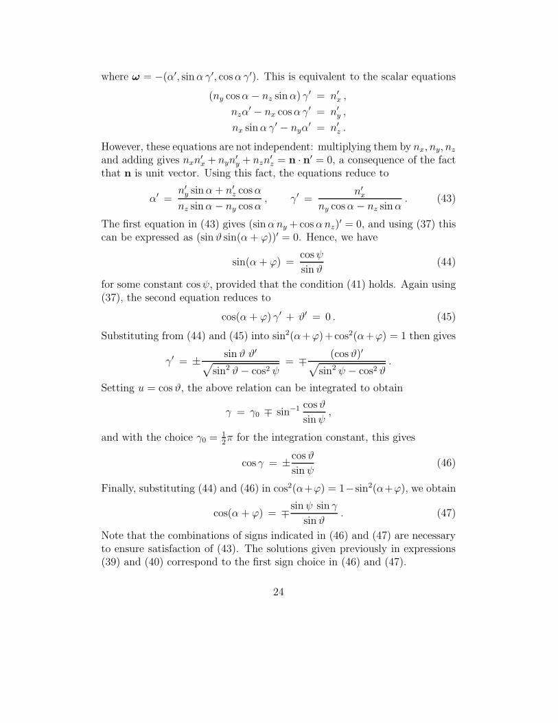
Figure 7 illustrates the inverse kinematics of an orientable–table machinefor a smooth path on a tensor–product bicubic NURBS surface, implemented

20

0.5 0.7 0.9 1.1 1.3 1.5–60o

–30o

0o

30o

60o

90o

120o

ξ

axis

rot

atio

n an

gle

γ

α

Figure 5: Variation of the rotary–axis angles γ, α along the path (30) on thetorus (29), computed from (39) and (40), for the orientable–table machine.

Figure 6: The toolpath (30) for ξ ∈ [ 1

2, 3

2] on the torus (29) for the case of an

orientable–table machine in Example 2. The position and orientation of thetorus vary continuously, such that the surface normal (shown as an arrow)at the tool contact point is a fixed vector in the machine coordinate system.

21

using the OpenNURBS and OpenSceneGraph software libraries. The surfaceparameter domain was normalized to (u, v) ∈ [ 0, 1 ]×[ 0, 1 ] and the tool pathr(ξ) = s(u(ξ), v(ξ)) was defined as a line segment in the parameter domain,between the points r(0) = s(0, 0) and r(1) = s(0.8, 0.8).

Figure 7: Variation of the workpiece orientation for a smooth toolpath r(ξ) ona bicubic NURBS surface. The workpiece orientations at the path parametervalues ξ = 0.0, 0.2, 0.4, 0.6, 0.8, 1.0 are shown, from top left to bottom right.

The limitation on the toolpaths incurred by the orientable–table machine,to ensure satisfaction of the condition (41), can be alleviated by re–fixturingthe workpiece on the machine table with a different orientation. However, useof multiple re–fixturings during machining operations is undesirable, becauseof inaccuracies they incur in registering the workpiece location/orientation.

7 Closure

The problem of determining the rotary–axis inputs to 5–axis CNC machines,so as to minimize variations of relative tool/workpiece orientation under theconstraint of a fixed cutting speed with a ball–end tool, has been addressed.The results of a prior study [6] can be directly applied to orientable–spindlemachines to determine the axis inputs, but since they depend on the integralof the geodesic curvature along the toolpath, a discrete time–step procedure

22

was proposed that offers sufficiently accurate real–time computation at thetypical sampling frequencies of modern 5–axis CNC machines.

The results of [6] require re–interpretation in the context of an orientable–table machine. In this case, the tool axis is stationary, and the minimizationof variations in the relative tool/workpiece orientation implies that the tableon which the workpiece is mounted must be continuously re–oriented so thatthe surface normal at the tool contact point becomes a static vector in themachine coordinate system. A closed–form solution for the rotary–axis inputsrealizing this motion is possible, that does not incur any irreducible integrals.However, the desired motion can only be realized when certain constraintson the variation of the surface normal along the toolpath are satisfied.

The elimination of “unnecessary” rotary–axis actuation in 5–axis CNCmachining of free–form surfaces, subject to toolpath geometry and cutting–speed constraints, can enhance the efficiency and accuracy of an expensiveand time–consuming fabrication process. The measure of optimality adoptedherein is essentially differential in nature — comparing the tool axis a andsurface normal n at the contact point, we require the component of one vectorparallel to the other to maintain the fixed value cosψ, while the perpendicularcomponent must exhibit no instantaneous rotation about the other.

The formulation of alternative measures of optimality, expressed in termsof a suitable combined metric for the rotary–axis inputs on a given machineconfiguration, is worthy of further detailed investigation.

Appendix

For a given unit vector n(ξ), let M(ξ) be a rotation matrix of the form (36)that maps n(ξ) into a fixed vector, i.e., n = Mn satisfies n′ = M′ n+Mn′ =0. Since M is an orthogonal matrix, this condition can be expressed as

MT M′ n + n′ = 0 . (42)

For the rotation matrix (36), one can verify that

MTM′ =

0 − γ′ cosα γ′ sinαγ′ cosα 0 −α′

− γ′ sinα α′ 0

,

and equation (42) can be re–written as

ω × n = n′ ,

23

where ω = −(α′, sinα γ′, cosα γ′). This is equivalent to the scalar equations

(ny cosα− nz sinα) γ′ = n′x ,

nzα′ − nx cosα γ′ = n′

y ,

nx sinα γ′ − nyα′ = n′

z .

However, these equations are not independent: multiplying them by nx, ny, nz

and adding gives nxn′x + nyn

′y + nzn

′z = n · n′ = 0, a consequence of the fact

that n is unit vector. Using this fact, the equations reduce to

α′ =n′

y sinα + n′z cosα

nz sinα− ny cosα, γ′ =

n′x

ny cosα− nz sinα. (43)

The first equation in (43) gives (sinαny + cosαnz)′ = 0, and using (37) this

can be expressed as (sinϑ sin(α+ ϕ))′ = 0. Hence, we have

sin(α + ϕ) =cosψ

sin ϑ(44)

for some constant cosψ, provided that the condition (41) holds. Again using(37), the second equation reduces to

cos(α + ϕ) γ′ + ϑ′ = 0 . (45)

Substituting from (44) and (45) into sin2(α+ϕ)+cos2(α+ϕ) = 1 then gives

γ′ = ±sin ϑ ϑ′

√

sin2 ϑ− cos2 ψ= ∓

(cosϑ)′√

sin2 ψ − cos2 ϑ.

Setting u = cosϑ, the above relation can be integrated to obtain

γ = γ0 ∓ sin−1 cosϑ

sinψ,

and with the choice γ0 = 1

2π for the integration constant, this gives

cos γ = ±cos ϑ

sinψ(46)

Finally, substituting (44) and (46) in cos2(α+ϕ) = 1−sin2(α+ϕ), we obtain

cos(α + ϕ) = ∓sinψ sin γ

sin ϑ. (47)

Note that the combinations of signs indicated in (46) and (47) are necessaryto ensure satisfaction of (43). The solutions given previously in expressions(39) and (40) correspond to the first sign choice in (46) and (47).

24

References

[1] R. L. Bishop (1975), There is more than one way to frame a curve,Amer. Math. Monthly 82, 246–251.

[2] C. Castagnetti, E. Duc, and P. Ray (2008), The domain of admissibleorientation concept: a new method for five–axis tool pathoptimisation, Comput. Aided Design 40, 938–950.

[3] H. I. Choi and C. Y. Han (2002), Euler–Rodrigues frames on spatialPythagorean–hodograph curves, Comput. Aided Geom. Design 19,603–620.

[4] R. T. Farouki (2010), Quaternion and Hopf map characterizations forthe existence of rational rotation–minimizing frames on quintic spacecurves, Adv. Comp. Math. 33, 331–348.

[5] R. T. Farouki, C. Giannelli, C. Manni, and A. Sestini (2012),Design of rational rotation–minimizing rigid body motions by Hermiteinterpolation, Math. Comp. 81, 879–903.

[6] R. T. Farouki and S. Li (2013), Optimal tool orientation control for5–axis CNC milling with ball-end cutters, Comput. Aided Geom.

Design 30, 226–239.

[7] I. D. Faux and M. J. Pratt (1979), Computational Goemetry for

Design and Mnaufacture, Ellis Horwood Ltd, Chichester.

[8] P. Gray, S. Bedi, and F. Ismail (2003), Rolling ball method for 5–axissurface machining, Comput. Aided Design 35, 347–357.

[9] H. Guggenheimer (1989), Computing frames along a trajectory,Comput. Aided Geom. Design 6, 77–78.

[10] M. C. Ho, Y. R. Hwang, and C. H. Hu (2003), Five–axis toolorientation smoothing using quaternion interpolation algorithm, Inter.

J. Mach. Tools Manuf. 43, 1259–1267.

[11] Y. R. Hwang and C. S. Liang (1998), Cutting error analysis forspindle–tilting type five–axis NC machines, Int. J. Adv. Manuf.

Technol. 14, 399–405.

25

[12] C. S. Jun, K. Cha, and Y. S. Lee (2003), Optimizing tool orientationsfor 5–axis machining by configuration–space search method, Comput.

Aided Design 35, 549–566.

[13] Y. H. Jung, D. W. Lee, J. S. Kim, and H. S. Mok (2002), NCpost–processor for 5–axis milling machine of table–rotating/tiltingtype, J. Mater. Proc. Tech. 130-131, 641–646.

[14] F. Klok (1986), Two moving coordinate frames for sweeping along a3D trajectory, Comput. Aided Geom. Design 3, 217–229.

[15] E. Kreyszig (1959), Differential Geometry, University of Toronto Press.

[16] R–S. Lee and C–H. She (1997), Developing a postprocessor for threetypes of five–axis machine tools, Int. J. Adv. Manuf. Technol. 13,658–665.

[17] Y. S. Lee (1997), Admissible tool orientation control of gougingavoidance for 5–axis complex surface machining, Comput. Aided

Design 29, 507–521.

[18] N. Rao, F. Ismail, and S. Bedi (1997), Tool path planning for five–axismachining using the principal axis method, Inter. J. Mach. Tools

Manuf. 37, 1025–1040.

[19] S. Sakamoto and I. Inasaki (1993), Analysis of generating motion forfive–axis machining centers, Trans. Jpn. Soc. Mech. Engr. Ser. C 59(561), 1553–1559.

[20] D. J. Struik (1988), Lectures on Classical Differential Geometry, DoverPublications (reprint), New York.

[21] W. Wang, B. Juttler, D. Zheng, and Y. Liu (2008), Computation ofrotation minimizing frames, ACM Trans. Graphics 27, No. 1, Article2, 1–18.

[22] A. Warkentin, F. Ismail, and S. Bedi (2000), Comparison betweenmulti–point and other 5–axis tool positioning strategies, Inter. J.

Mach. Tools Manuf. 40, 185–208.

26

[23] X. J. Xu, C. Bradley, Y. F. Zhang, H. T. Loh, and Y. S. Wong (2002),Tool–path generation for five–axis machining of free–form surfacesbased on accessibility analysis, Inter. J. Prod. Res. 40, 3253–3274.

27