University of Texas at El PasoDigitalCommons@UTEP

Open Access Theses & Dissertations

2019-01-01

Inverse Gaussian Ornstein-Uhlenbeck Applied ToModeling High Frequency DataEmmanuel Kofi KusiUniversity of Texas at El Paso

Follow this and additional works at: https://digitalcommons.utep.edu/open_etdPart of the Applied Mathematics Commons, and the Mathematics Commons

This is brought to you for free and open access by DigitalCommons@UTEP. It has been accepted for inclusion in Open Access Theses & Dissertationsby an authorized administrator of DigitalCommons@UTEP. For more information, please contact lweber@utep.edu.

Recommended CitationKusi, Emmanuel Kofi, "Inverse Gaussian Ornstein-Uhlenbeck Applied To Modeling High Frequency Data" (2019). Open Access Theses& Dissertations. 1997.https://digitalcommons.utep.edu/open_etd/1997

INVERSE GAUSSIAN ORNSTEIN - UHLENBECK APPLIED TO MODELING HIGH

FREQUENCY DATA.

EMMANUEL KOFI KUSI

Master’s Program in Mathematics

APPROVED:

Maria C. Mariani, Ph.D., Chair

Joe Guthrie, Ph.D.

T. Sarkodie Gyan, Ph.D.

Stephen Crites, Ph.D.Dean of the Graduate School

c©Copyright

by

Emmanuel Kofi Kusi

2019

to my

MOTHER and FATHER

with love

INVERSE GAUSSIAN ORNSTEIN - UHLENBECK APPLIED TO MODELING HIGH

FREQUENCY DATA.

by

EMMANUEL KOFI KUSI

THESIS

Presented to the Faculty of the Graduate School of

The University of Texas at El Paso

in Partial Fulfillment

of the Requirements

for the Degree of

MASTER OF SCIENCE

Department of Mathematical Sciences

THE UNIVERSITY OF TEXAS AT EL PASO

August 2019

Acknowledgements

My sincere gratitude goes to God Almighty for his guidance and confidence that has en-

abled me to complete this work successfully.

I would like to express my deep-felt gratitude to my advisor, Dr. Maria Christina Mariani

of the Mathematical Sciences Department at The University of Texas at El Paso, for her

advice, encouragement, enduring patience and constant support. She was never ceasing in

her belief in me (though I was often doubting in my own abilities), always providing clear

explanations when I was (hopelessly) lost, constantly driving me with energy I was tired,

and always giving me her time, in spite of anything else that was going on. Her response

to my verbal thanks one day was a very modest, “Excellent”. I wish all students the honor

and opportunity to experience her ability to perform at that job.

I also wish to thank the other members of my committee, Dr. Joe Guthrie of the Math-

ematical Sciences Department and Dr. T. Sarkodie Gyan of the Electrical & Computing

Engineering Department, both at The University of Texas at El Paso. Their suggestions,

comments and additional guidance were invaluable to the completion of this work.

As a special note, Osei Kofi Tweneboah graciously volunteered to act as my academic

mentor while He is also studying in PhD. Computational Sciences. He was extremely help-

ful in providing the additional guidance and expertise I needed in order to complete this

work, especially with regard to the chapter on Inverse Gaussian Ornstein Uhlenbeck model

and its application to Seismic and Market data.

Additionally, I want to thank The University of Texas at El Paso Mathematical Science

Department professors and staff for all their hard work and dedication, providing me the

v

means to complete my degree and prepare for a career as a mathematician. This includes

(but certainly is not limited to) the following individuals:

Dr. Amy Wagler

She made it possible for me to have many wonderful experiences I enjoyed while

a student, including the opportunity to teach beginning Mathematics students

the basics of R and Python (something I wish I had been taught when I first

started), and the ability to present

Dr. Joe Guthrie

His influence, though unbeknownst to him, was one of the main reasons for

coming to UTEP. He taught me Topology in semester I and I obtain Grade A

in His course.

And finally, I must thank my dear sister for putting up with me during the development

of this work with continuing, loving support and no complaint. I do not have the words to

express all my feelings here, only that I love you, Emelia!

vi

Abstract

With about 226050 estimated deaths worldwide in 2010, an earthquake is considered as

one of the disasters that records a great number of deaths. This thesis develops a model

for the estimation of magnitude of future seismic events.

We propose a stochastic differential equation arising on the Ornstein-Uhlenbeck processes

driven by IG(a,b) process. IG(a,b) Ornstein-Uhlenbeck processes offers analytic flexibil-

ity and provides a class of continuous time processes capable of exhibiting long memory

behavior. The stochastic differential equation is applied to geophysics and financial stock

markets by fitting the superposed IG(a,b) Ornstein-Uhlenbeck model to earthquake and

financial time series.

vii

Table of Contents

Page

Acknowledgements . . . . . . . . . . . . . . . . . . . . . . . . . . . . . . . . . . . . v

Abstract . . . . . . . . . . . . . . . . . . . . . . . . . . . . . . . . . . . . . . . . . . vii

Table of Contents . . . . . . . . . . . . . . . . . . . . . . . . . . . . . . . . . . . . . viii

List of Tables . . . . . . . . . . . . . . . . . . . . . . . . . . . . . . . . . . . . . . . xi

List of Tables . . . . . . . . . . . . . . . . . . . . . . . . . . . . . . . . . . . . . . . xi

List of Figures . . . . . . . . . . . . . . . . . . . . . . . . . . . . . . . . . . . . . . xii

List of Figures . . . . . . . . . . . . . . . . . . . . . . . . . . . . . . . . . . . . . . xii

Chapter

1 Introduction . . . . . . . . . . . . . . . . . . . . . . . . . . . . . . . . . . . . . . 1

1.1 Overview . . . . . . . . . . . . . . . . . . . . . . . . . . . . . . . . . . . . . 1

1.2 Background of the Study . . . . . . . . . . . . . . . . . . . . . . . . . . . . 1

1.3 Introduction of Earthquakes . . . . . . . . . . . . . . . . . . . . . . . . . . 3

1.4 Problem Statement . . . . . . . . . . . . . . . . . . . . . . . . . . . . . . . 4

1.5 Objectives of the study . . . . . . . . . . . . . . . . . . . . . . . . . . . . . 5

1.6 Methodology . . . . . . . . . . . . . . . . . . . . . . . . . . . . . . . . . . 5

1.7 Significance of the Study . . . . . . . . . . . . . . . . . . . . . . . . . . . . 5

1.8 Organization of Thesis . . . . . . . . . . . . . . . . . . . . . . . . . . . . . 6

2 Literature Review . . . . . . . . . . . . . . . . . . . . . . . . . . . . . . . . . . . 7

2.1 Stochastic and Levy Processes . . . . . . . . . . . . . . . . . . . . . . . . 7

2.1.1 Examples of Stochastic and Levy Processes . . . . . . . . . . . . . . 8

2.1.2 Properties of Stochastic and Levy Processes . . . . . . . . . . . . . 16

2.2 Subordination of Levy process . . . . . . . . . . . . . . . . . . . . . . . . . 22

2.3 The Levy - Ito Decomposition: Structure of the Sample Paths of Levy Pro-

cesses . . . . . . . . . . . . . . . . . . . . . . . . . . . . . . . . . . . . . . 22

viii

2.4 Deterministic Differential Equations . . . . . . . . . . . . . . . . . . . . . . 23

2.5 Stochastic Differential Equations . . . . . . . . . . . . . . . . . . . . . . . 24

2.5.1 Ito Integral . . . . . . . . . . . . . . . . . . . . . . . . . . . . . . . 26

2.5.2 Properties of the Ito integral . . . . . . . . . . . . . . . . . . . . . . 27

2.6 Ito process, Ito formula . . . . . . . . . . . . . . . . . . . . . . . . . . . . . 27

2.6.1 Multidimensional Ito formula . . . . . . . . . . . . . . . . . . . . . 28

2.7 Seismic Events and Financial Markets : The Source of High

Frequency Data . . . . . . . . . . . . . . . . . . . . . . . . . . . . . . . 29

3 Methodology . . . . . . . . . . . . . . . . . . . . . . . . . . . . . . . . . . . . . 31

3.1 Introduction . . . . . . . . . . . . . . . . . . . . . . . . . . . . . . . . . . . 31

3.1.1 Arithmetic Brownian motion . . . . . . . . . . . . . . . . . . . . . . 31

3.1.2 Geometric Brownian motion . . . . . . . . . . . . . . . . . . . . . . 32

3.2 Definition and existence of Ornstein-Uhlenbeck Process . . . . . . . . . . . 33

3.3 Solution of the Ornstein-Uhlenbeck Processes . . . . . . . . . . . . . . . . 34

3.4 Inverse Gaussian Ornstein Uhlenbeck - Model and Parameter Estimation . 35

3.4.1 Estimation of the shape parameter a and rate parameter b of the

IG(a,b) Ornstein - Uhlenbeck Model . . . . . . . . . . . . . . . . . 35

3.4.2 Estimation the mean reverting parameter λ of the IG(a,b) Ornstein

- Uhlenbeck Model . . . . . . . . . . . . . . . . . . . . . . . . . . . 35

3.4.3 Estimation of the arrival times of a Poisson Process

N = (Ns)s≥0 of rate λ for the IG(a,b) - OU simulation . . . . . . . 36

4 Model Formulation and Numerical Simulation . . . . . . . . . . . . . . . . . . . 37

4.1 Introduction . . . . . . . . . . . . . . . . . . . . . . . . . . . . . . . . . . . 37

4.2 The Inverse Gaussian OU model . . . . . . . . . . . . . . . . . . . . . . . . 38

4.3 Simulation techniques . . . . . . . . . . . . . . . . . . . . . . . . . . . . . . 38

4.4 Simulation via the inverse tail mass function . . . . . . . . . . . . . . . . . 39

5 Model Simulations and Analysis . . . . . . . . . . . . . . . . . . . . . . . . . . . 45

5.1 Analysis of geophysical time series . . . . . . . . . . . . . . . . . . . . . . . 45

ix

5.2 Chile earthquake time series . . . . . . . . . . . . . . . . . . . . . . . . . . 45

5.3 Financial time series . . . . . . . . . . . . . . . . . . . . . . . . . . . . . . 48

5.3.1 Real Data Analysis of Chile Data . . . . . . . . . . . . . . . . . . . 48

5.3.2 Real Data Analysis of Financial indices . . . . . . . . . . . . . . . . 50

5.3.3 Discussion of Numerical Results . . . . . . . . . . . . . . . . . . . . 50

6 Concluding Remarks . . . . . . . . . . . . . . . . . . . . . . . . . . . . . . . . . 51

6.1 Introduction . . . . . . . . . . . . . . . . . . . . . . . . . . . . . . . . . . . 51

6.2 Conclusion . . . . . . . . . . . . . . . . . . . . . . . . . . . . . . . . . . . . 51

6.3 Recommendation . . . . . . . . . . . . . . . . . . . . . . . . . . . . . . . . 52

6.4 Significance of the Result . . . . . . . . . . . . . . . . . . . . . . . . . . . . 52

6.5 Future Work . . . . . . . . . . . . . . . . . . . . . . . . . . . . . . . . . . . 52

References . . . . . . . . . . . . . . . . . . . . . . . . . . . . . . . . . . . . . . . . . 54

Curriculum Vitae . . . . . . . . . . . . . . . . . . . . . . . . . . . . . . . . . . . . . 57

x

List of Tables

2.1 Moments of the Poisson distribution with intensity λ . . . . . . . . . . . . 11

2.2 Moments of the Γ(a, b) distribution . . . . . . . . . . . . . . . . . . . . . . 12

2.3 Moments of the IG(a, b) distribution . . . . . . . . . . . . . . . . . . . . . 14

2.4 Moments of the GIG(λ, a, b) distribution . . . . . . . . . . . . . . . . . . . 15

4.1 Parameter Descriptions for Chile Earthquake Data . . . . . . . . . . . . . 40

4.2 Chile Data Results for Superposed Γ(a, b) Ornstein - Uhlenbeck model with

∆t = 0.0001 . . . . . . . . . . . . . . . . . . . . . . . . . . . . . . . . . . . 40

4.3 Chile Data Results for Inverse Gaussian IG (a,b) Ornstein - Uhlenbeck model

with ∆t = 0.0001 . . . . . . . . . . . . . . . . . . . . . . . . . . . . . . . . 43

4.4 Chile Data Results for Superposed Γ(a, b) OU - model with X0 = X1 +X2 43

4.5 Parameter Descriptions for Emergent / Developed Market Asian Crises Data 43

4.6 Emergent and Developed Stock Markets Data Results for Inverse Gaussian

IG (a,b) Ornstein-Uhlenbeck model with ∆t = 0.0001 . . . . . . . . . . . . 44

5.1 Parameter Descriptions for Chile Data . . . . . . . . . . . . . . . . . . . . 48

5.2 Numerical results for the IG(λ, a, b) OU model . . . . . . . . . . . . . . . . 49

xi

List of Figures

2.1 Random Walk . . . . . . . . . . . . . . . . . . . . . . . . . . . . . . . . . . 9

2.2 Simulation of Poisson Process . . . . . . . . . . . . . . . . . . . . . . . . . 10

2.3 The solutions Xt = X0et to the random differential equation dXt = Xtdt

with initial condition X0 = eN , where N has an N(0, σ2) distribution with

σ2 = 0.01 and 0.0001 respectively . . . . . . . . . . . . . . . . . . . . . . . 25

4.1 ρ(1) = 0.1133 . . . . . . . . . . . . . . . . . . . . . . . . . . . . . . . . . . 41

4.2 ρ(1) = 0.0453 . . . . . . . . . . . . . . . . . . . . . . . . . . . . . . . . . . 41

4.3 ρ(1) = 0.1950 . . . . . . . . . . . . . . . . . . . . . . . . . . . . . . . . . . 41

4.4 ρ(1) = 0.1951 . . . . . . . . . . . . . . . . . . . . . . . . . . . . . . . . . . 41

4.5 ∆t = 0.0001 . . . . . . . . . . . . . . . . . . . . . . . . . . . . . . . . . . . 42

4.6 ∆t = 0.0001 . . . . . . . . . . . . . . . . . . . . . . . . . . . . . . . . . . . 42

4.7 ∆t = 0.0001 . . . . . . . . . . . . . . . . . . . . . . . . . . . . . . . . . . . 42

4.8 ∆t = 0.0001 . . . . . . . . . . . . . . . . . . . . . . . . . . . . . . . . . . . 42

5.1 Region 1 . . . . . . . . . . . . . . . . . . . . . . . . . . . . . . . . . . . . . 46

5.2 Region 2 . . . . . . . . . . . . . . . . . . . . . . . . . . . . . . . . . . . . . 46

5.3 Region 3 . . . . . . . . . . . . . . . . . . . . . . . . . . . . . . . . . . . . . 47

5.4 Region 4 . . . . . . . . . . . . . . . . . . . . . . . . . . . . . . . . . . . . . 47

xii

Chapter 1

Introduction

1.1 Overview

In this chapter I present the background of the study, the problem statement, the objectives

of the study, the methodology, the justification (significance of the study) and finally the

organization of the study.

1.2 Background of the Study

Seismic Hazard analyses involve the quantitative estimation of ground - shaking at a partic-

ular site. Seismic hazards may be analyzed deterministically, as when a specific earthquake

scenario is assumed, or probabilistically, in which uncertainties in the size, location and

time of occurrence of the earthquake are explicitly considered. There are a lot of researches

and analyses currently going globally concerning the geophysical mechanisms that drive

seismic events and so of today, a quite number of mathematical models which explore the

time of occurrence and earthquake magnitude on a particular site is said to be stochasti-

cally dependent.

The motivation for studying this problem comes from continuous stochastic volatility mod-

els in financial mathematics. Barndorff - Nielsen and Shephard(2001, 2003) model stock

price as a geometric Brownian motion and the diffusion coefficient of this motion as an

Ornstein- Uhlenbeck (OU) process that is driven by the Levy process which is (nonnega-

tive and nondecreasing). In the field of Geophysics and Finance, distributions of returns

1

from turbulent wind speed and financial assets can often be fitted very well by the Inverse

Gaussian distribution. It is therefore of some interest, using the inverse Gaussian laws as

building blocks to construct Ornstein-Uhlenbeck models on seismic and financial data.

It is therefore suitable to model phenomena where large values are more probable than

any other cases. For Stock market returns and prices, a key characteristic is that it models

that extremely large variations from typical (crashes) can occur even when almost all (nor-

mal) variations are small. With these areas of application in mind, mainly those of finance,

we study in recent papers several kind of processes with the Inverse Gaussian marginals,

in particular processes of Ornstein - Uhlenbeck type, superpositions of such processes and

stochastic volatility models in one, two and several dimensions.

But for the purpose of this project, we will consider to find models with analytically and

statistically correlation structure to the occurrences of seismic and financial events. And the

feasibility of carrying out likelihood inference under the derived models will be discussed to

some extent. The next three chapters discuss important ideas and theorems. In chapter 2,

there are some pre - requisites for better understanding of the project which would be given

under the preliminaries. This chapter contains various preliminaries, mostly well known,

results concerning: Inverse Gaussian distributions; Infinite divisibility and exponential fam-

ilies; Self - decomposability; Ornstein - Uhlenbeck type processes and Background Driving

Levy processes; long range dependence and self - similarity; stochastic volatility and the

processes of Inverse Gaussian type.

We would then move to the main body of the work; where we then define the Inverse

Gaussian Ornstein - Uhlenbeck process and we characterize the associated BDLP as the

sum of two homogeneous Levy processes, one being the inverse Gaussian Levy process and

the second a Gamma Levy process.

2

Chapter 4 discusses the simulation methods and the analysis of the seismic data and dis-

cussion of findings. Chapter 5 investigate the model formulation and the analysis of the

Inverse-Gaussian OU model and the Gamma OU model by comparison of these model us-

ing the seismic data and stock markets data. Finally we shall give conclusion of our work,

summary and some recommendations in Chapter 6.

1.3 Introduction of Earthquakes

An earthquake is the sudden movement of the ground that releases elastic energy stored

in rocks and generates seismic waves. The elastic energy can be built up and stored over

a long time and then released in seconds or minutes. Strain on the rocks results in more

elastic energy being stored which leads to far greater possibility of an earthquake event.

The sudden release of energy during an earthquake causes low-frequency sound waves called

seismic waves to propagate through the earth’s crust or along its surface. These elastic

waves radiate outward from the ”source” and vibrate the ground.

Direct Shaking Hazards and Human-Made Structures

Most earthquake-related deaths are caused by the collapse of structures and the construc-

tion practices play a tremendous role in the death toll of an earthquake. In southern Italy

in 1909 more than 100,000 people perished in an earthquake that struck the region. Almost

half of the people living in the region of Messina were killed due to the easily collapsible

structures that dominated the villages of the region. A larger earthquake that struck San

Francisco three years earlier had killed fewer people (about 700) because building con-

struction practices were different type (predominantly wood). Survival rates in the San

Francisco earthquake was about 98%, that in the Messina earthquake was between 33%

and 45% (Zebrowski, 1997). Building practices can make all the difference in earthquakes,

even a moderate rupture beneath a city with structures unprepared for shaking can produce

tens of thousands of casualties.

3

Although probably the most important, direct shaking effects are not the only hazard as-

sociated with earthquakes, other effects such as landslides, liquefaction, and tsunamis have

also played important part in destruction produced by earthquakes.

In an earthquake, the initial movement that causes seismic vibrations occurs when two

sides of a fault suddenly slide pass each other. A fault is a large fracture in rocks, across

which the rocks have moved. There are three main types of faults, all of which may cause

an interplate earthquake namely, normal, reverse (thrust) and strike-slip. An interplate

earthquake is an earthquake that occurs at the boundary between two tectonic plates.

Earthquakes of this type account for more than 90% of the total seismic energy released

around the world . Plate tectonics is the theory that earth’s outer shell is divided into

several plates that glide over the mantle, the rocky inner layer above the core. The plates

act like a hard and rigid shell compared to the earth’s mantle. The strong outer layer is

called the lithosphere. If one plate is trying to move pass the other, they will be locked until

sufficient stress builds up to cause the plates to slip relative to each other. The slipping

process creates an earthquake with land deformations and resulting seismic waves which

travel through the earth and along the earth’s surface.

1.4 Problem Statement

It has always been a problem for people to estimate future seismic hazards of a particular

region. There are quite a number of models which explore the occurrences of future seismic

events where the prediction of time, location and magnitude focused on the magnitude

of the future seismic events as well as the effects of the seismic hazards. There are few

publications on the estimation of the magnitude hazards and its progression to earthquakes

of a region. One of the few is by (Maria et al; 2015) which analyzed the Stochastic

Differential Equations of Earthquakes Series. There is the need to extend their work to

include a new model and to determine the necessary ingredients for the simulation process.

4

1.5 Objectives of the study

The objectives of the study includes the following;

• To construct an Inverse Gaussian OU model following Maria et al(2016) of the

stochastic differential equations applied to high frequency data in Geophysics.

• To perform the (magnitude of future seismic events) Data analysis of the model.

• To perform simulations to determine the effect of varying the model.

• Comparison of these 2 OU model (Inverse Gaussian OU model and Gamma OU

model).

1.6 Methodology

In this study, an Ornstein - Uhlenbeck processes driven by IG(a,b) process is developed to

investigate the magnitude of earthquake and its effects in a particular region.

We begin by developing the dynamics of Levy processes and Inverse Gaussian OU model

adapted from Mariani et al 2015. The Self decomposability of the new stochastic dif-

ferential equations which takes into account earthquake is well investigated. Finally we

perform simulation on the solution of the proposed stochastic differential equation using

MATLAB.

1.7 Significance of the Study

This study is a step towards understanding the relevance of properties such as Ornstein -

Uhlenbeck processes that characterize the estimation of future stochastic events. A clear

understanding of the impact of earthquakes as in the magnitude of earthquakes and making

suggestion in promoting the prevention of impact of certain regions in the future.

5

1.8 Organization of Thesis

This study is organized into five chapters and outlined as follows:

1. Introduction: This chapter presents a general introduction to the study with a

background to the study, the problem statement, objectives, methodology and the

significance of the study.

2. Literature Review: In this chapter various literatures with relation to history,

Ornstein-Uhlenbeck processes, mathematical models and application of control are

presented.

3. Methodology: This chapter discusses various methods adopted for the study with

a focus on definitions as well as a case study.

4. Model Formulation and Analysis: In this chapter, the model is formulated. The

Inverse Gaussian OU model and Gamma OU model are also well investigated.

5. Analysis and Simulations: In this chapter, the magnitude of the model are com-

puted using parameter values from the simulations of the earthquake time series and

market crises which are also presented and the results discussed.

6. Conclusion and Recommendations: This chapter concludes the entire study

and lays out some recommendations for future studies.

6

Chapter 2

Literature Review

In this chapter, a reviewed literature on the history of OU processes is presented. Some

literatures are also presented on two types of OU processes as well as various works on

stochastic and levy processes. Literatures on mathematical models related to earthquakes

and stock markets are also presented.

2.1 Stochastic and Levy Processes

Definition 1. A stochastic process is a family of random variables X(t) : tεT, where

t usually denotes time. That is, at every time t in the set T , a random number X(t) is

observed.

Stochastic processes are widely used as mathematical models of systems and phenom-

ena that appear to vary in a random manner. They have applications in many disciplines

including sciences such as biology, chemistry, ecology, neuroscience, and physics as well as

technology and engineering fields such as image processing, signal processing, information

theory, computer science, cryptography and telecommunications. Furthermore, seemingly

random changes in financial markets have motivated the extensive use of stochastic pro-

cesses in finance.

Definition 2. A cadlag stochastic process Y = Ytt≥0 with Y0 = 0 is a Levy process if

and only if it has independent and (strictly) stationary increments .

Levy processes are types of stochastic processes that can be considered as generalizations

of random walks in continuous time. These processes have many applications in fields such

7

as finance, fluid mechanics, physics and biology. The main defining characteristics are their

stationarity and independence properties with stationary and independent increments.

2.1.1 Examples of Stochastic and Levy Processes

In this section, we will present some examples of Stochastic and Levy Processes. Then,

we look at processes that live on the real line. We shall pay attention also to their density

function, their characteristic function, their Levy triplets, together with some of their

properties. We compute moments, variance, skewness and kurtosis, if possible.

The Weiner Process

A stochastic process W = Wt, t ≥ 0 is a Weiner process (Brownian motion) if the following

conditions holds:

i. W0 = 0.

ii. W has stationary increments, i.e. the distribution of the increment Wt+s −Wt over

the interval [t, t+ s].

iii. W has independent increments; i.e. if 1 < s ≤ t < u, Wu −Wt and Ws −Wl are

independent random variables. In other words, increments over non - overlapping

time intervals are stochastically independent.

iv. For 0 ≤ s < t, Wt+s−Wt follows normal distribution with mean 0 and variance s > 0:

Wt+s −Wt ∼ Normal(0,s).

The Random Walk

Let Yk, k ≥ 1, be i.i.d. Then

Sn =n∑k=1

Yk, n ∈ N

is a random walk.

8

Figure 2.1: Random Walk

Random walks are stochastic processes that are usually defined as sums of independent

and identically distributed(iid) random variables in Euclidean space so they are processes

that change in discrete time. Random walks can also be referred processes that change in

continuous time, particularly the Wiener process used in finance, which has led to some

confusion, resulting in its criticism. There are other various types of random walks, defined

so their state spaces can be other mathematical objects, such as lattices and groups, and

in general they are highly studied and have many applications in different disciplines.

A classic example of a random walk is known as the simple random walk, which is a

stochastic process in discrete time with the integers as the state space, and is based on a

Bernoulli process, where each Bernoulli variable takes either ±1.

The Bernoulli Process

One of the simplest stochastic processes is the Bernoulli process, which is a sequence of

independent and identically distributed random variables, where each random variable

takes either the value one or zero, say one with probability 1 − p. This process can be

linked to repeatedly flipping a coin, where the probability of obtaining a head is p and its

9

value is one, while the value of a tail is zero.

The Poisson Process

The Poisson process is the simplest Levy Processes we can think of. It is based on the Pois-

son distribution, which depends on a single parameter λ and has the following characteristic

function:

φPoisson(u;λ) = exp(λ(exp(iu)− 1))

The Poisson distribution lives on the nonnegative integers j = 0, 1, 2, ...; the probability

mass function at point j is given by;

f(j, λ) =λje−λ

j!

Since the Poisson(λ) distribution is infinitely divisible, we can define N = Nt, t ≥ 0

with intensity parameter λ > 0 as the process which starts at 0, has independent and

stationary increments and where the increment over a time interval of length δ > 0 follows

a Poisson(λs) distribution. The Poisson process turns out to be an increasing pure jump

process, with jump sizes always equal to 1.

Figure 2.2: Simulation of Poisson Process

10

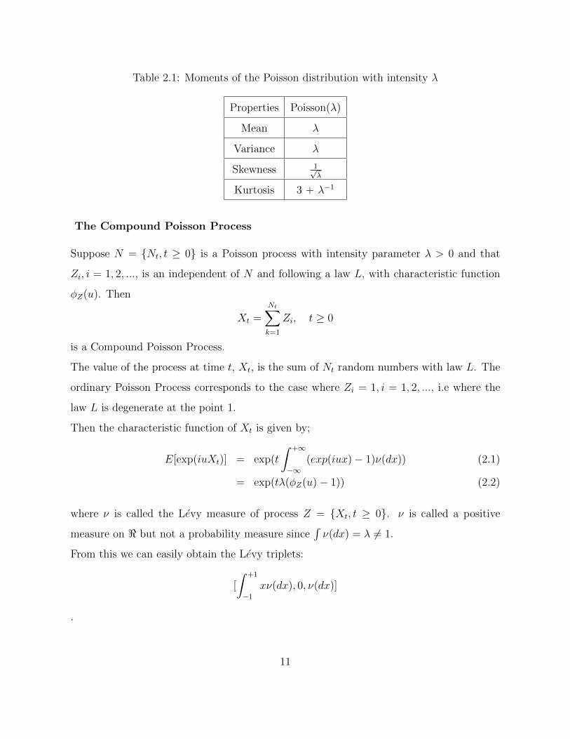
Table 2.1: Moments of the Poisson distribution with intensity λ

Properties Poisson(λ)

Mean λ

Variance λ

Skewness 1√λ

Kurtosis 3 + λ−1

The Compound Poisson Process

Suppose N = Nt, t ≥ 0 is a Poisson process with intensity parameter λ > 0 and that

Zi, i = 1, 2, ..., is an independent of N and following a law L, with characteristic function

φZ(u). Then

Xt =Nt∑k=1

Zi, t ≥ 0

is a Compound Poisson Process.

The value of the process at time t, Xt, is the sum of Nt random numbers with law L. The

ordinary Poisson Process corresponds to the case where Zi = 1, i = 1, 2, ..., i.e where the

law L is degenerate at the point 1.

Then the characteristic function of Xt is given by;

E[exp(iuXt)] = exp(t

∫ +∞

−∞(exp(iux)− 1)ν(dx)) (2.1)

= exp(tλ(φZ(u)− 1)) (2.2)

where ν is called the Levy measure of process Z = Xt, t ≥ 0. ν is called a positive

measure on < but not a probability measure since∫ν(dx) = λ 6= 1.

From this we can easily obtain the Levy triplets:

[

∫ +1

−1

xν(dx), 0, ν(dx)]

.

11

The Gamma Process

The density function of the Gamma distribution Γ(a, b) with parameters a > 0 and b > 0

is given by;

fGamma(x; a, b) =ba

Γ(a)xa−1 exp(−xb), x > 0

The density function clearly has a semi - heavy (right) tail. The characteristic function is

given by;

φGamma(u; a, b) = (1− iu/b)−a

This characteristic function is infinitely divisible. The Gamma processX(Gamma) = X(Gamma)t , t ≥

0 with the stochastic process which starts at zero and has stationary and independent

Gamma distributed increments where X(Gamma)t follows a Γ(at, b) distribution.

The Levy triplet of the Gamma process is given by;

[a(1− exp(−b))/b, 0, a exp(−bx)x−11(x>0)dx]

Table 2.2: Moments of the Γ(a, b) distribution

Properties Γ(a, b)

Mean a/b

Variance a/b2

Skewness 2a−1/2

Kurtosis 3(1 + 2a−1)

The Inverse Gaussian Process

Let T (a,b) be the first time a standard Brownian motion with drift b > 0, i.e. Ws+bs, s ≥ 0,

reaches the positive level a > 0. It is well known that this random time follows the so -

called Inverse - Gaussian IG(a, b) law and has a characteristics function

φIG(u; a, b) = exp(−a√−2iu+ b2 − b).

12

The IG distribution is infinitely divisible and we define the IG process X(IG) = XIGt , t ≥

0, with parameters a, b > 0, as the process which starts at 0 and has independent and

stationary increments such that

E[exp(iuX(IG)t )] = φIG(u; at, b) (2.3)

= exp(−at(√−2iu+ b2)− b)). (2.4)

The density function of the IG(a, b) is explicitly known:

fIG(x; a, b) =a√2π

exp(ab)x−3/2 exp(−1

2(a2x−1 + b2x)), x > 0

The Levy measure of the IG(a, b) law is given by;

νIG(dx) = (2π)−1/2ax−3/2 exp(−1

2b2x)1(x>0)dx

and the first component of the Levy triplet equals

γ =a

b(2N(b)− 1),

where the N(x) is the Normal distribution function.

Properties

The density is unimodal with a mode at (√

4a2b2+9−3)(2b2)

. All positive and negative moments

exist. If X follows on IG(a, b) law, we have that

E[X−α] = (b

a)2α+1E[Xα+1], α ∈ R

The Generalized Inverse Gaussian Process

The Inverse Gaussian IG(a, b) law can be generalized to what is called the Generalized

Inverse Gaussian distribution GIG(λ, a, b). This distribution on the positive half line is

given in terms of its density function.

fGIG(x;λ, a, b) =(b/a)λ

2Kλ(ab)xλ−1 exp(−1

2(a2x−1 + b2x)), x > 0

13

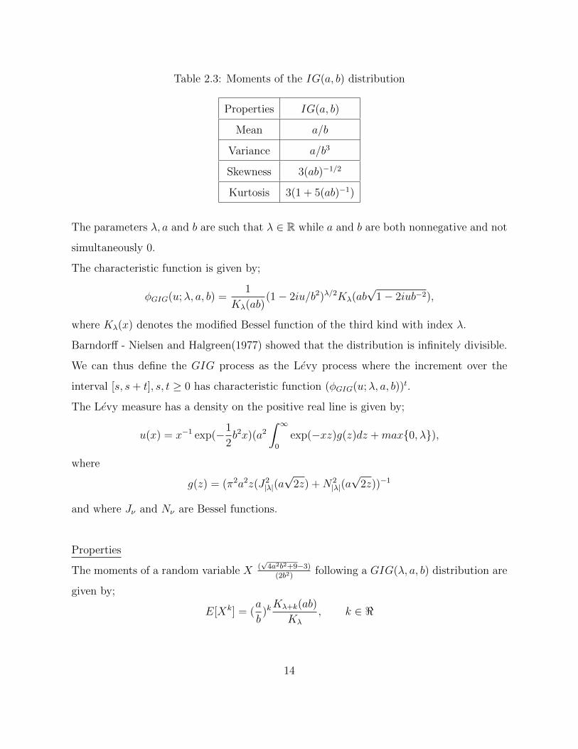
Table 2.3: Moments of the IG(a, b) distribution

Properties IG(a, b)

Mean a/b

Variance a/b3

Skewness 3(ab)−1/2

Kurtosis 3(1 + 5(ab)−1)

The parameters λ, a and b are such that λ ∈ R while a and b are both nonnegative and not

simultaneously 0.

The characteristic function is given by;

φGIG(u;λ, a, b) =1

Kλ(ab)(1− 2iu/b2)λ/2Kλ(ab

√1− 2iub−2),

where Kλ(x) denotes the modified Bessel function of the third kind with index λ.

Barndorff - Nielsen and Halgreen(1977) showed that the distribution is infinitely divisible.

We can thus define the GIG process as the Levy process where the increment over the

interval [s, s+ t], s, t ≥ 0 has characteristic function (φGIG(u;λ, a, b))t.

The Levy measure has a density on the positive real line is given by;

u(x) = x−1 exp(−1

2b2x)(a2

∫ ∞0

exp(−xz)g(z)dz +max0, λ),

where

g(z) = (π2a2z(J2|λ|(a√

2z) +N2|λ|(a√

2z))−1

and where Jν and Nν are Bessel functions.

Properties

The moments of a random variable X (√

4a2b2+9−3)(2b2)

following a GIG(λ, a, b) distribution are

given by;

E[Xk] = (a

b)kKλ+k(ab)

Kλ

, k ∈ <

14

Table 2.4: Moments of the GIG(λ, a, b) distribution

Properties GIG(λ, a, b)

Mean aKλ+1(ab)/(bKλ(ab))

Variance a/b2

Martingale

In probability theory, a martingale is a stochastic process (i.e, a sequence of random vari-

ables) such that the conditional expected value of an observation at some time t, given all

the observations up to some earlier time s, is equal to the observation at that earlier time

s.

A discrete-time martingale is discrete-time stochastic process X1, X2, X3, ...that satisfies for

all n

E(| Xn |) <∞

E(Xn+1 | X1, ..., Xn) = Xn

i.e, the conditional expected value of the next observation, given all the past observations,

is equal to the last observation.

Somewhat more generally, a sequence Y1, Y2, Y3, ... is said to be a martingale with respect

to another X1, X2, X3, ...

E(| Yn |) <∞

E(Yn+1 | X1, ..., Xn) = Yn.

Similarly, a continuous-time martingale with respect to the stochastic process Xt is a

stochastic process Yt such that for all t.

E(| Yt |) <∞

E(Yt | Xτ , τ ≤ s) = Ys,∀s ≤ t.

15

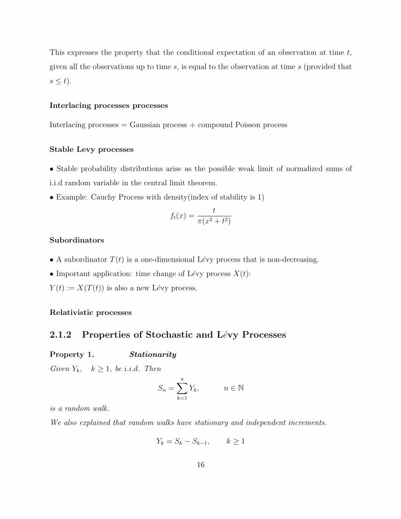
This expresses the property that the conditional expectation of an observation at time t,

given all the observations up to time s, is equal to the observation at time s (provided that

s ≤ t).

Interlacing processes processes

Interlacing processes = Gaussian process + compound Poisson process

Stable Levy processes

• Stable probability distributions arise as the possible weak limit of normalized sums of

i.i.d random variable in the central limit theorem.

• Example: Cauchy Process with density(index of stability is 1)

ft(x) =t

π(x2 + t2)

Subordinators

• A subordinator T (t) is a one-dimensional Levy process that is non-decreasing.

• Important application: time change of Levy process X(t):

Y (t) := X(T (t)) is also a new Levy process.

Relativistic processes

2.1.2 Properties of Stochastic and Levy Processes

Property 1. Stationarity

Given Yk, k ≥ 1, be i.i.d. Then

Sn =n∑k=1

Yk, n ∈ N

is a random walk.

We also explained that random walks have stationary and independent increments.

Yk = Sk − Sk−1, k ≥ 1

16

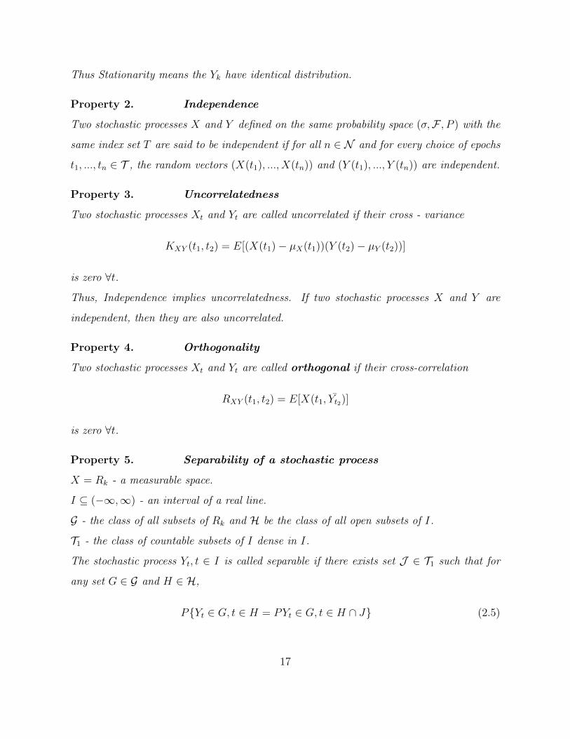
Thus Stationarity means the Yk have identical distribution.

Property 2. Independence

Two stochastic processes X and Y defined on the same probability space (σ,F , P ) with the

same index set T are said to be independent if for all n ∈ N and for every choice of epochs

t1, ..., tn ∈ T , the random vectors (X(t1), ..., X(tn)) and (Y (t1), ..., Y (tn)) are independent.

Property 3. Uncorrelatedness

Two stochastic processes Xt and Yt are called uncorrelated if their cross - variance

KXY (t1, t2) = E[(X(t1)− µX(t1))(Y (t2)− µY (t2))]

is zero ∀t.

Thus, Independence implies uncorrelatedness. If two stochastic processes X and Y are

independent, then they are also uncorrelated.

Property 4. Orthogonality

Two stochastic processes Xt and Yt are called orthogonal if their cross-correlation

RXY (t1, t2) = E[X(t1, Yt2)]

is zero ∀t.

Property 5. Separability of a stochastic process

X = Rk - a measurable space.

I ⊆ (−∞,∞) - an interval of a real line.

G - the class of all subsets of Rk and H be the class of all open subsets of I.

T1 - the class of countable subsets of I dense in I.

The stochastic process Yt, t ∈ I is called separable if there exists set J ∈ T1 such that for

any set G ∈ G and H ∈ H,

PYt ∈ G, t ∈ H = PYt ∈ G, t ∈ H ∩ J (2.5)

17

Thus, relation (2.5) is equivalent to the relation

PAG,H,J\AG,H = 0

The set J is called a set of separability for the process Yt.

Lemma 1.1. Let Yt, t ∈ I is a real - valued process. Then it is separable, if for any open

interval (a, b) ⊆ I

P supa<t<b

Yt = supa<t<b,t∈I

Yt = P infa<t<b

Yt = infa<t<b,t∈J

Yt = 1

Example 1. The process Yt = I(t = ρ), t ∈ I is not separable while the process Zt ≡ I is

separable and any set J ∈ T1 is the set of separability for the process.

Example 2. The process ω(t) = ω(t)I(t 6= τ), t > 0 is not separable while the process

ω(t), t ≥ 0 is separable and any set J ∈ T(0,∞) is the set of separability for this process.

Let X = Rk and Rk = [−∞,∞]× ...× [−∞,∞] be an extended Euclidean space Rk.

Property 6. Stochastic continuity of a stochastic process

A stochastic process Yt, t ∈ I with the phase space Rk is stochastically continuous in the

point t0 ∈ I,

P| Yt − Yt0 |> δ → 0 as t→ t0, δ > 0

Therefore, the process Yt, t ∈ I is stochastically continuous if it is stochastically continuous

in every point t0 ∈ I.

Theorem 2.1. If the process Yt, t ∈ I with the phase space Rk is stochastically continuous,

then there exists a separable modification Zt, t ∈ I for the process Yt such that any set

J ∈ T1 is a separability set for the process Zt.

Example 1. The process Yt = I(t = ρ), t ∈ I is not separable but it is a stochastically

continuous process. Any set J ∈ T1 is a separability set for the separable modification

Zt ≡ 0, t ∈ I for the process Zt.

18

Example 2. The process ω(t) = ω(t)I(t 6= τ), t > 0 is not separable but it is a stochastically

continuous process. Any set J ∈ T[0,∞) is the set of separability for the separable modification

ω(t), t ≥ 0 for the process ω(t).

Property 7. Indistinguishable

Two stochastic processes X and Y defined on the same probability space (Ω,F , P ) with the

same index set T and set space S are said to indistinguishable if following

P (Xt = Yt ∀t ∈ T ) = 1,

holds. If two X and Y are modifications of each other and are almost surely continuous,

then X and Y are indistinguishable.

Property 8. Modification

A modification of a stochastic process is another stochastic process, which is closely related

to the original stochastic process. More precisely, a stochastic process X that has the same

index set T , set space S, and probability space (Ω,F , P ) as another stochastic process Y is

said to be a modification of Y if for all t ∈ T the following

P (Xt = Yt) = 1,

holds. Two stochastic processes that are modifications of each other have the same law and

they are said to be stochastically equivalent.

Property 9. Stochastic volatility

Stochastic volatility is the main concept used in the fields of financial economics and math-

ematical finance to deal with endemic time-varying volatility and codependence found in

financial markets. Such dependence has been known for a long time, early comments in-

clude Mandelbrot (1963) and Officer (1973).

Our motivation for studying this research comes from continuous stochastic volatility models

in financial mathematics. Stochastic volatility models provide a basis for realistic modeling

19

of option prices. Thus, It is the time-change by an integrated stationary volatility process,

e.g. OU processes driven by subordinators Xt:

Yt = exp−λtY0 +

∫ t

0

exp−λ(t− s)dXλs

It =

∫ t

0

Ysds

Zt = BIt

This model is by Barndorff-Nielsen and Shephard. This and others can be simulated and

used for option pricing.

Property 10. Infinite divisibility

Suppose Y := Ytt≥0 is a Levy process on Rd, then for all t > 0, Y must be divisible into

n ≥ 2 i.i.d random variables

Yt =n∑k=1

(Ytk/n − Yt(k−1)/n),

since Yt since these are successive increments (independent) of equal length(stationary).

Property 11. Self - decomposability

Given λ as a positive number. Then, an infinitely divisible distribution FY is called self-

decomposable, if there exists a random variable X = Xt,λ, such that, for each t ∈ R+;

φFY(u) = φFY

(e−λtu)φFXu, u ∈ R

where φFY(u) and φFX

(u) are the characteristic functions corresponding to FY and FXcorresponding.

If∫|x|>1

log(|x|)FL(dx) <∞, then the class of all possible invariant distributions of Y forms

the class of all self-decomposable distributions FY with the background driven Levy driven

process L.

Theorem 2.2. Let v(dx) denote the Levy measure of an infinitely divisible measure F on

R. Then the following statements are equivalent:

20

1. F is self-decomposable.

2. The functions on the positive half-line given by v((−∞,−es]) and v([es,∞)) are both

convex.

3. v(dx) is of the form v(dx) = u(x)dx with |x|u(x) increasing on (−∞, 0) and decreas-

ing on (0,∞).

21

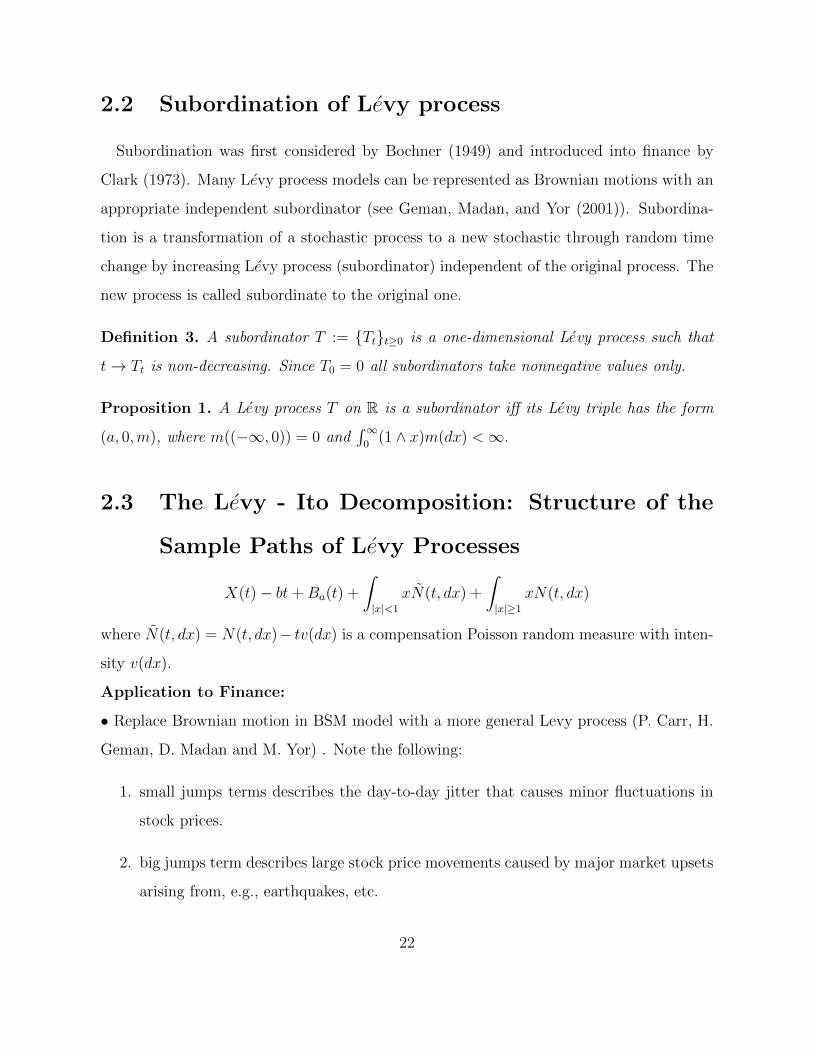
2.2 Subordination of Levy process

Subordination was first considered by Bochner (1949) and introduced into finance by

Clark (1973). Many Levy process models can be represented as Brownian motions with an

appropriate independent subordinator (see Geman, Madan, and Yor (2001)). Subordina-

tion is a transformation of a stochastic process to a new stochastic through random time

change by increasing Levy process (subordinator) independent of the original process. The

new process is called subordinate to the original one.

Definition 3. A subordinator T := Ttt≥0 is a one-dimensional Levy process such that

t→ Tt is non-decreasing. Since T0 = 0 all subordinators take nonnegative values only.

Proposition 1. A Levy process T on R is a subordinator iff its Levy triple has the form

(a, 0,m), where m((−∞, 0)) = 0 and∫∞

0(1 ∧ x)m(dx) <∞.

2.3 The Levy - Ito Decomposition: Structure of the

Sample Paths of Levy Processes

X(t)− bt+Ba(t) +

∫|x|<1

xN(t, dx) +

∫|x|≥1

xN(t, dx)

where N(t, dx) = N(t, dx)− tv(dx) is a compensation Poisson random measure with inten-

sity v(dx).

Application to Finance:

• Replace Brownian motion in BSM model with a more general Levy process (P. Carr, H.

Geman, D. Madan and M. Yor) . Note the following:

1. small jumps terms describes the day-to-day jitter that causes minor fluctuations in

stock prices.

2. big jumps term describes large stock price movements caused by major market upsets

arising from, e.g., earthquakes, etc.

22

Main problems with Levy Processes in Finance

• Market is incomplete, i.e. there may be more than one possible pricing formula.

• One of the methods to overcome the problems associated with Levy Processes in Finance

is the entropy minimization.

Example; hyperbolic Levy process(E. Eberlain) (with no Brownian motion part); a pricing

formula have been developed that has minimum entropy.

2.4 Deterministic Differential Equations

A differential equation is a mathematical equation that relates some function of one or

more variables with its derivatives. Differential equations arise whenever a deterministic

relation involving some continuously varying quantities (modeled by functions) and their

rates of change in space and/or time (expressed as derivatives) is known or postulated.

Because such relations are extremely common, differential equations play a prominent role

in many disciplines including engineering, physics, economics, and biology.

Differential equations are mathematically studied from several different perspectives,

mostly concerned with their solutions - the set of functions that satisfy the equation.

Only the simplest differential equations are solvable by explicit formulas; however, some

properties of solutions of a given differential equation may be determined without finding

their exact form. If a self-contained formula for the solution is not available, the solution

may be numerically approximated using computers. The theory of dynamical systems

puts emphasis on qualitative analysis of systems described by differential equations, while

many numerical methods have been developed to determine solutions with a given degree

of accuracy.

A deterministic (ordinary) differential equation is an equation involving a function (of

one variable) and its derivatives. They are essential for a mathematical description of na-

ture - they lie at the core of many physical theories. For example, let us just Newton’s

23

and Lagrange’s equations for classical mechanics, Maxwell’s equations for classical electro-

magnetism, Schrodinger’s equation for quantum mechanics, and Einstein’s equation for the

general theory of gravitation.

Examples:

(a) Newton’s law: Mass times acceleration equals force, ma = f , where m is the

particle mass, a = d2x/dt2 is the particle acceleration, and f is the force acting on the

particle. Hence Newton’s law is the differential equation

md2x

dt2(t) = f(t, x(t),

dx

dt(t)),

where the unknown is x(t)− the position of the particle in space at the time t. As

we see above, the force may depend on time, on the particle position in space, and

on the particle velocity.

(b) Radioactive Decay: The amount u of a radioactive material changes in time as

follows,du

dt(t) = −ku(t), k > 0,

where k is a positive constant representing radioactive properties of the material.

(c) The Heat Equation: The temperature T in a solid material changes in time and

in three space dimensions-labeled by x = (x, y, z)− according to the equation

∂T

∂t(t, x) = k(

∂2T

∂x2(t, x) +

∂2T

∂y2(t, x) +

∂2T

∂z2(t, x)), k > 0,

2.5 Stochastic Differential Equations

A stochastic differential equation(SDE) is a differential equation in which one or more of

the terms is a stochastic process resulting in a solution which is itself a stochastic process.

Consider the deterministic diffferential equation:

dx(t) = k(t, x(t))dt, x(0) = x0. (2.6)

24

The easiest way to introduce randomness in the equation is to randomize the initial condi-

tion. The solution x(t) then becomes a stochastic process Xt, t ∈ [0, T ]:

dXt = k(t,Xt)dt, X0(ω) = Y (ω). (2.7)

Such an equation is called a random differential equation. Random differential equations

can be considered as a deterministic equation with a perturbed initial condition. The

investigation is of great interest if we study the robustness of the solution to a differential

equation under a small change of the initial condition.

Figure 2.3: The solutions Xt = X0et to the random differential equation dXt = Xtdt with

initial condition X0 = eN , where N has an N(0, σ2) distribution with σ2 = 0.01 and 0.0001

respectively

In this section, the randomness in the differential equation is introduced via an addi-

tional random noise term:

dXt = k(t,Xt)dt+ b(t,Xt)dBt, X0(ω) = Y (ω) (2.8)

25

B = (Bt, t ≥ 0) denotes Brownian motion, and k(t, x) and l(t, x) are deterministic func-

tions. The process X, if it exists, is then a stochastic process. The randomness of

X = (Xt, t ∈ [0, T ]) is as a result of the initial condition and the noise generated by

Brownian motion.

Interpretation of Equation 2.8 tells us that the change dXt = Xt+dt −Xt is caused by a

change dt of time, with factor b(t,Xt). Since the Brownian motion, with factor k(t,Xt) in

a combination with a change dBt = Bt+dt − Bt of Brownian motion, with factor l(t,Xt).

Since the Brownian motion does not have differentiable sample paths, the question that

normally arises is in which sense can we interpret Equation (2.8). Applying integration on

both sides of Equation (2.8), we obtain

Xt = X0 +

∫ t

0

k(s,Xs)ds+

∫ t

0

l(s,Xs)dBs, 0 ≤ t ≤ T, (2.9)

Where the first integral on the right-hand side is a Riemann integral, and the second one

is a Ito stochastic process satisfying Equation (2.9).

We will proceed to prove the existence, in a certain sense of∫ t

0

f(s, ω)dBs(ω) (2.10)

where Bt(ω) is a 1-dimensional Brownian motion starting at the origin, for a wide class of

functions f : [0,∞]× Ω→ R.

2.5.1 Ito Integral

We continue with the construction of Ito integral using the following propositions.

Proposition 2. Suppose a sequence of simple processes Xn satisfies (1). There exists a

process Zt ∈ M2,c satisfying limnE[(Zt − It(X n))2] = 0 for all 0 ≤ t ≤ T . This process is

unique a.s. in the following sense: if Xnt is another process satisfying (1) and Z is the

corresponding limit, then P (Zt = Zt,∀t ∈ [0, T ]) = 1.

26

Now we can formally state the definition of Ito integral.

Definition 1 (Ito integral). Given a stochastic process Xt ∈ L2 and T > 0, its Ito

integral It(X), t ∈ [0, T ] is defined to be the unique process Zt constructed in proposition 2.

We have defined Ito integral as a process which is defined for all t ≥ 0, by taking T →∞

and taking approximate limits.

2.5.2 Properties of the Ito integral

Theorem 2.5.2. Let f, g ∈ V (S, T ) and let 0 ≤ S < U < T . Then

1.∫ TSfdBt =

∫ USfdBt +

∫ TUfdBt.

2.∫ TS

(cf + g)dBt = c∫ TSfdBt +

∫ TSgdBt, for c ∈ R.

3. E[(∫ TSfdBt)] = 0.

4.∫ TSfdBt is FT −measurable.

2.6 Ito process, Ito formula

An Ito process or stochastic integral is a stochastic process on (Ω,F , P ) adopted to Ftwhich can be written in the form

Xt = X0 +

∫ t

0

Usds+

∫ t

0

VsdBs (2.11)

where U, V ∈ L2. As a shorthand notation, we will write (equation 11) as

dXt = Utdt+ VtdBt

Ito formula

In the previous sections, we have observed that a sample Brownian path is nowhere differ-

entiable with probability 1. In other words, the differentiation

dBt

dt

27

does not exist. However, while studying Brownian motions, or when using Brownian motion

as a model, the situation of estimating the difference of a function of the type

f(Bt)

over an infinitesimal time difference occurs quite frequently (suppose that f is a smooth

function). To be more precise, we are considering a function f(t, Bt) which depends only on

the second variable. Hence there exists an implicit dependence on time since the Brownian

motion depends on time.

We now introduce the most important formula of Ito calculus:

Theorem 1 (Ito formula). Let Xtbe an Ito process dXt = Utdt + VtdBt. Suppose

g(x) ∈ C2(R) is a twice continuously differentiable function (in particular all second partial

derivatives are continuous functions). Suppose g(Xt) ∈ L2. Then Yt = g(Xt) is again an

Ito process and

dYt =∂g

∂x(Xt)dXt +

1

2

∂2g

∂x2(Xt)(dXt)

2

Using the notational convention for dXt = Utdt+ VtdBt and (dXt)2, we can rewrite the

Ito formula as

dYt = (∂g

∂x(Xt)Ut +

1

2

∂2g

∂x2(Xt)V

2t )dt+

∂g

∂x(Xt)VtdBt.

Thus, we see that the space of Ito processes is closed under twice - continuously differen-

tiable transformations.

2.6.1 Multidimensional Ito formula

There is a very useful analogue of Ito formula in many dimensions. Before turning to the

formula we need to extend our discussion to the case of Ito processes with respect to many

dimensions, as so far we have considered Ito integrals and Ito processes with respect to

just one Brownian motion. Thus suppose we have a vector of d independent Brownian

motions Bt = (Bi,t, 1 ≤ i ≤ d, t ∈ R+). A stochastic process Xt is defined to be an Ito

28

process with respect to Bt if there exists Ut ∈ L2 and Vi,t ∈ L2, 1 ≤ i ≤ d such that

Xt = Utdt+∑

i Vi,tdBi,t, in the sense explained above.

Theorem 2.. Suppose dXt = Utdt + VtdBt, where vector U = (U1, ..., Ud) and matrix

V = (V11, ..., Vdd) have L2 components and B is the vector of d independent Brownian

motions. Let g(x) be twice continuously differentiable function from Rd into R. Then

Yt = g(Xt) is also an Ito process and

dYt =d∑i=1

∂g

∂xi(Xt)dXi,t +

1

2

d∑i,j=1

∂2g

∂xixj(Xt)dXi,t · dXj,t,

where dXi,t · dXj,t is computed using the rules dtdt = dtdBt = dBidt = 0, dBidBj for all

i 6= j and (dBi)2 = dt.

2.7 Seismic Events and Financial Markets : The Source of High

Frequency Data

A famous climber, when asked why he was willing to put his life in danger to climb

dangerous summits, answered : “Because they are there”. We would be tempted to give

the same answer when people ask us why we take so much pain in dealing the high -

frequency data. The reason is very simple: Financial markets and Seismic occurrences are

the source of high frequency data.

By its very nature it is irregularly spaced in time, however, and with the sheer volume

being reported by liquid markets can only be understood using continuous dynamics (Hanif

and Protopapas, 2013). Financial data providers usually report hundreds of thousands of

prices for a single market a day.

Dacorogna et al.(2001) argue, correctly, that high frequency data should be primary

object of research for those who are interested in understanding seismic events such as

(Floods, explosions, earthquakes), and financial markets, especially given the effect of mar-

ket dynamics on everyday investors.

29

Yet, most of the published papers and studies in the field of geophysics and finance deal

with a lower frequency, regularly spaced data because of these two reasons:

Firstly, it is costly and resource-intensive to collect, store, manipulate and curate high fre-

quency data.This is precisely why most available data is either daily or lower frequencies.

The second season is somehow more subtle but still quite important: most of the statistical

apparatus has been developed and thought for homogeneous (equally spaced in time) time

series. Nowadays with the development of computer technology, data availability is becom-

ing less and less of as problem.Little work has been done to look into irregular data with

(Hanif and Protopapas, 2013), described above, working towards bridging the gap between

regularized and irregular time series.

30

Chapter 3

Methodology

3.1 Introduction

The aim of this chapter is to discuss the methods adopted for this study. Therefore, this

chapter focuses on the necessary ingredients for the simulation process which entails the

Ornstein - Uhlenbeck process introduced by [] for modeling the volatility coefficient in a

stock price process that follows a geometric Brownian motion. We will discuss modeling

issues of Levy driven OU processes and present some simulation results.

Definition 1. A stochastic process is a family of random variables X(t) : tεT, where

t usually denotes time. That is, at every time t in the set T , a random number X(t) is

observed.

3.1.1 Arithmetic Brownian motion

A Brownian motion with drift is called arithmetic Brownian motion(ABM). The actual

model of ABM is a stochastic differential equation (SDE) of this form;

dX = µdt+ σdz

. The model has two parameters;

1. Drift

2. Volatility (sometime also known as the diffusion coefficient)

31

3.1.2 Geometric Brownian motion

In the modeling of seismic data and financial market, especially earthquake series and

stock market, Brownian Motion play a significant role in building a statistical model. In

this section, we will explore some of the technique to build a seismic and financial model

called the Inverse Gaussian Ornstein-Uhlenbeck model using Brownian Motion and write

our Matlab code for simulation and model building.

Before the building our code in Matlab, we will introduce some concepts here in order

to understand the in depth process of Brownian Motion in the Ornstein-Uhlenbeck model.

Definition 2. A stochastic process St is said to follow a Geometric Brownian Motion if it

satisfies the following stochastic differential equation:

dSt = µStdt+ σStWt (3.1)

Where Wt is a Wiener process(Brownian Motion) and µ, σ are constants.

Normally, µ is called the percentage drift and σ is called the percentage volatility. So,

consider Brownian motion trajectory that satisfy the differential equation, the right hand

side term µStdt controls the ”trend” of this trajectory and the term σStdWt controls the

”random noise” effect in the trajectory.

Since it is a differential equation, we want to find a solution by applying the separation

of variables technique, then the equation (3.1) becomes:

dStSt

= µdt+ σWt (3.2)

Then take the integration of both side∫dStSt

=

∫(µdt+ σdWt)dt (3.3)

32

Since dSt

Strelates to derivative of ln(St), then the equation (3.3) involving the Ito calculus

gives us equation (3.4);

ln(dStSt

) = (µ− 1

2σ2)t+ σWt (3.4)

Taking the exponential of both side of equation (3.4) and plugging the initial condition

S0, we obtain the solution. The analytical solution of this geometric brownian motion

(equation (3.1)) is given by:

St = S0exp((µ−σ2

2)t+ σWt)

Thus, the process above is of solving a stochastic differential equation, and in fact,

geometric brownian motion is defined as a stochastic differential equation.

3.2 Definition and existence of Ornstein-Uhlenbeck

Process

A continuous time stationary and non-negative stochastic process X = X(t) is said to

be an Ornstein - Uhlenbeck process if it satisfies the stochastic differentiation

dX(t) = −λX(t) + σdL(t)

X(0) = X0

where L = L(t) is a Gaussian process with mean 0 and variance tσ2, λ is a strictly

positive intensity parameter and X0 is an independent random variable. One possible

generalization of this process emerges from allowing L to be a Levy process. Such a model

is called a process of Ornstein - Uhlenbeck type. The L is termed as the background driving

Levy process (BDLP).

33

In our work, we will be mainly interested in stationary processes of this type, which

can be generated by imposing certain conditions to the BDLP L or more interestingly by

designing a stationary self-decomposable law, say D, and finding then a BDLP L that

exactly matches this distribution.

3.3 Solution of the Ornstein-Uhlenbeck Processes

As the OU process is used to model mean reverting behavior, we have λ > 0 and t > 0;

The solution of the stochastic differential equation (SDE) can be found by applying Ito’s

lemma to V (t,Xt) = eλtXt

The Ito’s Lemma

d(v(t,Xt)) = [∂V

∂t(t,Xt) + a(t,Xt)

∂V

∂Xt

(t,Xt) +1

2(b(t,Xt))

2 ∂2V

∂X2t

d(t,Xt)]dt+ b(t,Xt)∂V

∂Xt

dLt

d(eλtXt) = [λXteλt − λXte

λt]dt+ eλtLt

= eλtLt

Time integration gives then

eλtXt −Xt =

∫ t

0

eλsLs

Dividing through by eλt yields,

Xt = eλtX0 +

∫ t

0

eλ(t−s)dLs

for the initial condition X0 = x0.

34

3.4 Inverse Gaussian Ornstein Uhlenbeck - Model and

Parameter Estimation

3.4.1 Estimation of the shape parameter a and rate parameter b

of the IG(a,b) Ornstein - Uhlenbeck Model

We also need to know how the parameters µ and σ2 relate to a and b.

Proposition 3. Suppose that Ltt≥0 is a Levy process such that E(L(1)) = µ < ∞ and

V ar(L(1)) = σ2 < ∞. Let M be the largest constant satisfying Equation ... and assume

that λ > 0. Then the following holds:

1. E(X0) = µ

2. V ar(X0) = σ2

2

We have that

a = µ

√2µ

σ2and b =

√2µ

σ2(3.5)

3.4.2 Estimation the mean reverting parameter λ of the IG(a,b)

Ornstein - Uhlenbeck Model

Regarding the λ parameter, we recall our estimators: In order to estimate the mean re-

verting parameter λ, we begin with the definition of the autocorrelation function for the

process given in Equation 3.4 which is of the form,

ρ(h) = corr(Xt+h, Xt) = e−λh, for h ∈ N

λ = − loge ρ(h)

without loss of generality, we take h = 1. The our estimated intensity parameter is

λ = −log(ρ(1)) (3.6)

35

3.4.3 Estimation of the arrival times of a Poisson Process

N = (Ns)s≥0 of rate λ for the IG(a,b) - OU simulation

Theorem 3.1. For a Poisson process of rate λ, and for any t > 0, the PMF for N(t)

(i.e the number of arrivals in (0, t]) is given by the Poisson PMF,

PN(t)(n) =(λt)n exp(−λt)

n!(3.7)

Therefore the arrival times of a Poisson Process for our simulation is given by;

ci =(λt)i exp(−λt)

i!

where c1 < c2 < c3 < ... with intensity parameter ab2

.

36

Chapter 4

Model Formulation and Numerical

Simulation

4.1 Introduction

In this section we discuss modeling issues of Levy driven Ornstein -Uhlenbeck processes and

present some simulation results for an inverse Gaussian OU process. We use the simulated

data to test the performance for the simulation process.

A very important ingredient in modeling of Levy driven OU processes is the connection

between the Levy density of the stationary distribution of X to the Levy density of the

probability law of L1. In particular we have the following proposition.

Proposition 4. Assume that the Levy density of X, vX(z), is differentiable and denote the

Levy density of the probability law of L1 by vX(z). Then the following relation holds.

vL(x) = −vX(x)− xv′

X(x). (4.1)

Proof. It follows directly by the fact that the stationary solution, X, to (3.1) satisfies

X =D

∫ ∞0

e−λsdL(λs).

Hence, given vL(x) we can find vY (x) and vice versa.

37

4.2 The Inverse Gaussian OU model

An Ornstein-Uhlenbeck process X = (Xt)t≥0 is a decision of the stochastic differential

equation

dXt = −λXtdt+ dLλt, X0 > 0

We denote the Levy measure of L1 by W (dz) such that Levy density u(z) of the marginal

law D be differentiable, then the Levy measure W has a density w(z), and u(z) and w(z)

are related by

w(z) = −u(z)− zu′(z)

We define the tail mass function of W(dz) as:

W+(z) =

∫ ∞z

w(y)dy

The inverse function of W+(z) is of the form:

W−1(z) = infy > 0 : W+(y) ≤ z

We develop the Inverse Gaussian OU model using the inverse tail mass function. Thus the

Invere Gaussian OU process by the series representation via the inverse tail mass function

can be represented using the following approximation.

4.3 Simulation techniques

In this section, the inverse Gaussian OU model developed earlier using the inverse tail mass

function. Simulations are performed using Matlab based on the solution of our proposed

stochastic differential equation.

X(t) = X0e−λt +

∫ t

0

e−λ(t−s)dLλs (4.2)

= X0e−λt + e−λt

∫ t

0

esdLλ (4.3)

38

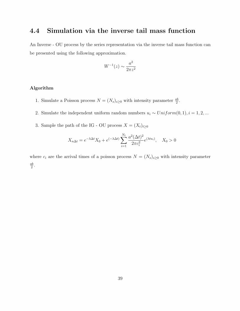
4.4 Simulation via the inverse tail mass function

An Inverse - OU process by the series representation via the inverse tail mass function can

be presented using the following approximation.

W−1(z) ∼ a2

2πz2

Algorithm

1. Simulate a Poisson process N = (Ns)s≥0 with intensity parameter ab2

.

2. Simulate the independent uniform random numbers ui ∼ Uniform(0, 1), i = 1, 2, ...

3. Sample the path of the IG - OU process X = (Xt)t≥0

Xn∆t = e−λ∆tX0 + e(−λ∆t)

Nt∑i=1

a2(∆t)2

2πc2i

e(λtui), X0 > 0

where ci are the arrival times of a poisson process N = (Ns)s≥0 with intensity parameter

ab2

.

39

Table 4.1: Parameter Descriptions for Chile Earthquake Data

Regions Number of Observations λ a b µ σ2

Region 1 389 2.1766 27.0669 5.8736 4.6082 0.2671

Region 2 1167 3.0955 29.8684 6.5759 4.5421 0.2101

Region 3 892 1.6348 26.3897 5.7509 4.5888 0.2775

Region 4 5000 1.6344 30.3151 6.7865 4.4670 0.1940

Table 4.2: Chile Data Results for Superposed Γ(a, b) Ornstein - Uhlenbeck model with

∆t = 0.0001

Regions λ1 λ2 X1 X2 w1 w2 RMSE

Region 1 2.1766 2.9766 4.3000 4.5000 0.5000 0.5000 0.1066

Region 2 3.0955 4.6150 4.0000 4.5000 0.4000 0.6000 0.0948

Region 3 1.6348 2.3480 4.7000 4.6000 0.4500 0.5500 0.1017

Region 4 1.6344 2.6344 4.6000 4.5000 0.4000 0.6000 0.0941

40

Figure 4.1: ρ(1) = 0.1133 Figure 4.2: ρ(1) = 0.0453

Figure 4.3: ρ(1) = 0.1950 Figure 4.4: ρ(1) = 0.1951

41

Figure 4.5: ∆t = 0.0001 Figure 4.6: ∆t = 0.0001

Figure 4.7: ∆t = 0.0001 Figure 4.8: ∆t = 0.0001

42

Table 4.3: Chile Data Results for Inverse Gaussian IG (a,b) Ornstein - Uhlenbeck model

with ∆t = 0.0001

Regions λ = − log(ρ(1)) X0 = Xn∆t Root Mean Square Error

Region 1 2.1766 4.6000 0.1041

Region 2 3.0955 4.5000 0.0952

Region 3 1.6348 4.6000 0.1077

Region 4 1.6344 4.5000 0.0935

Table 4.4: Chile Data Results for Superposed Γ(a, b) OU - model with X0 = X1 +X2

Regions λ1 λ2 X1 X2 w1 w2 RMSE

Region 1 2.1766 2.9766 4.2000 5.0000 0.5000 0.5000 0.1054

Region 2 3.0955 4.6150 4.0000 5.0000 0.4000 0.6000 0.1149

Region 3 1.6348 2.3480 4.5000 4.7000 0.4500 0.5500 0.1201

Region 4 1.6344 2.6344 4.4000 4.6000 0.4000 0.6000 0.3499

Table 4.5: Parameter Descriptions for Emergent / Developed Market Asian Crises Data

No. of

Indices Observations λ a b µ σ2

IGPA 806 0.0021 700.7189 0.1513 4.6304e+03 4.0493e+05

NASDAQ 2727 7.7324e-04 83.2849 0.1047 795.1966 1.4498e+05

SETI 1059 0.0074 108.6003 0.2887 376.1272 9.0234e+03

XU100 1014 0.0032 196.6306 0.0253 7.7622e+03 2.4193e+07

MXX 2476 0.0015 182.0223 0.0486 3.7452e+03 3.1711e+06

MERVAL 1250 0.2285 120.0396 0.2184 549.5960 2.3042e+04

BOVESPA 2100 0.0017 213.9919 0.0254 8.4349e+03 2.6211e+07

HSI 2674 0.0021 384.9144 0.0383 1.0052e+04 1.3712e+07

43

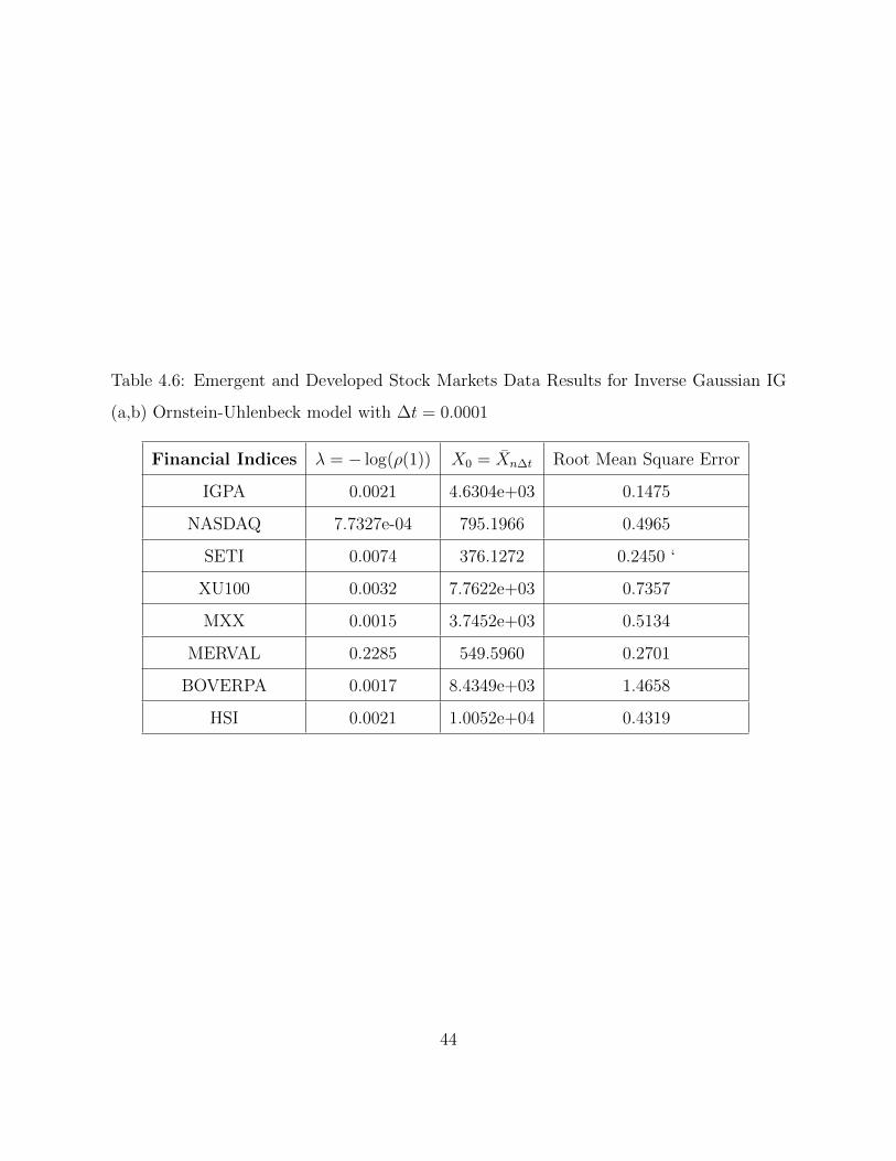
Table 4.6: Emergent and Developed Stock Markets Data Results for Inverse Gaussian IG

(a,b) Ornstein-Uhlenbeck model with ∆t = 0.0001

Financial Indices λ = − log(ρ(1)) X0 = Xn∆t Root Mean Square Error

IGPA 0.0021 4.6304e+03 0.1475

NASDAQ 7.7327e-04 795.1966 0.4965

SETI 0.0074 376.1272 0.2450 ‘

XU100 0.0032 7.7622e+03 0.7357

MXX 0.0015 3.7452e+03 0.5134

MERVAL 0.2285 549.5960 0.2701

BOVERPA 0.0017 8.4349e+03 1.4658

HSI 0.0021 1.0052e+04 0.4319

44

Chapter 5

Model Simulations and Analysis

5.1 Analysis of geophysical time series

In this chapter, the Inverse Gaussian OU model developed earlier in chapter 4 is analyzed

by using the fitted model applied to real seismic data series from Chile. We normalized the

data sets, by taking the logarithm of the time series data point. Then we also simulated

independent paths of our model using different time steps for the data sets. Simulations

are performed using Matlab to vary model variables and assess the estimated parameters.

We compared our model, that is the IG(a, b) Ornstein - Uhlenbeck model to Γ(a, b)

Ornstein- Uhlenbeck model to check which of them best fits the data. In order to in-

vestigate our model fit, we computed the root mean square error for each region. The root

mean square error indicates how well fitted is our model with respect to the given data

set. The solution to our stochastic differential equation is a Levy model, so the very good

fitting obtained strengthens the previous results.

5.2 Chile earthquake time series

The high frequency geophysical data was obtained from 4 regions in Chile from the year

2000 to 2014. The data contain information about the location of events, date, and mag-

nitudes of each 42 recorded earthquake in the region. The 4 regions under study were

selected based on the fact that it recently generated macro- earthquakes (Mw ≥ 8). The

sizes of the regions were selected according to the distribution of aftershocks after the

45

largest mega-earthquakes. Region 3 is of much interest since it shows clear fore-shocks.

Figures 4.1,4.2,4.3 and 4.4 shows the map of the 4 regions under study. The earthquakes

magnitude is the recorded data used in our analysis.

Figure 5.1: Region 1 Figure 5.2: Region 2

46

Figure 5.3: Region 3 Figure 5.4: Region 4

47

5.3 Financial time series

We studied emergent market indices corresponding to eight countries: Brazil (BOVESPA),

from 04-27-1993 to 10-22-2001; Argentina (MERVAL), from 10-8-1996 to 10-22-2001 and

Hong Kong (HSI), from 01-2-1991 to 10-25-2001, USA, Thailand, Turkey, Mexico, Ar-

gentina. The number of data points for BOVESPA, MERVAL and 2100,1250 and 2675

respectively. We also analyzed the Standard and Poor’s 500 (S & P 500), a major index of

the New York Stock Exchange. In the latter case, the data corresponds to a period from

01-3-1950 to 06-14-2005 with 13,951 data points. The daily close values were used in our

analyses.

5.3.1 Real Data Analysis of Chile Data

Table 5.1 and Table 5.2 summarize the results of the estimation of parameters for the

Inverse Gaussian Ornstein - Uhlenbeck model and Γ(a, b) Ornstein - Uhlenbeck model.

We obtained the following parameters: intensity parameter(λ), shape parameter(a), scale

parameter(b), mean(µ) and variance (σ2) of the data sets for each of the four regions.

Table 5.1: Parameter Descriptions for Chile Data

Regions Number of Observations λ a b µ σ2

Region 1 389 2.1766 27.0669 5.8736 4.6082 0.2671

Region 2 1167 3.0955 29.8684 6.5759 4.5421 0.2101

Region 3 892 1.6348 26.3897 5.7509 4.5888 0.2775

Region 4 5000 1.6344 30.3151 6.7865 4.4670 0.1940

48

Table 5.2: Numerical results for the IG(λ, a, b) OU model

Regions λ = − log(ρ(1)) X0 = Xn∆t Root Mean Square Error

Region 1 2.1766 4.6000 0.1041

Region 2 3.0955 4.5000 0.0952

Region 3 1.6348 4.6000 0.1077

Region 4 1.6344 4.5000 0.0935

49

5.3.2 Real Data Analysis of Financial indices

Table 4.5 and Table 4.6 summarize the results of the estimation of parameters for the Inverse

Gaussian Ornstein - Uhlenbeck model. We obtained the following parameters: intensity

parameter(λ), shape parameter(a), scale parameter(b), mean(µ) and variance (σ2) of the

data sets for the various countries.

5.3.3 Discussion of Numerical Results

In this project, we applied our model to time series arising in geophysics. This section

describes the source of our data sets and also present the numerical simulation results

when our model is applied to the data sets.

• The data set on earthquakes was obtained from the four regions in Chile from the

year 2000 to 2014

• The Inverse-Gaussian Ornstein Uhlenbeck model performed better than the Gamma

Ornstein Uhlenbeck model due to the compared results of the simulation.

50

Chapter 6

Concluding Remarks

6.1 Introduction

In this chapter, conclusions are drawn from the study and various recommendations are

made.

6.2 Conclusion

We implemented flexible classes of processes that incorporate long - range dependence, i.e

they have a slowly polynomially decaying autocovariance function and self - similarity like

properties and that are capable of describing some of the key distributional features of

typical geophysical and financial time series.

We constructed an independent IG(a, b) Ornstein-Uhlenbeck processes and simulated data

from our proposed model: Inverse Gaussian Ornstein-Uhlenbeck processes to estimate the

magnitude of the earthquake for the four regions in Chile. We compared our numerical

results to the Γ(a, b) Ornstein-Uhlenbeck process.

Based on the numerical results we obtained; the root mean square error, the IG(a, b)

Ornstein-Uhlenbeck process performed better than the Γ(a, b) Ornstein-Uhlenbeck process.

Likewise, for the time series using on financial indices near a crash for both well developed

and emergent markets, we estimated the daily closing values which is good to capture the

dynamics of the stock market.

In the previous works [14, 15], the authors concluded that the generalized Levy models

were very suitable to describe critical events including financial crashes and earthquakes.

51

The solution to our stochastic differential equation is a Levy model, so the very model

fitting obtained reinforces the previous conclusions.

6.3 Recommendation

Based on the study, the following recommendations are made;

1. The Inverse - Gaussian Ornstein Uhlenbeck model can be a basis for extending the

work to include spatial and structural aspects which could involve the use of stochastic

differential equations.

2. An optimal control analyses of the model can also be formulated to optimize the costs

and effectiveness of the control measures.

3. We conclude that the generalized Levy models are very suitable to describe critical

events including financial crashes and earthquakes.

6.4 Significance of the Result

Inverse Gaussian Ornstein-Uhlenbeck processes provide a class of continuous tine processes

which exhibit a long memory behavior. The presence of long memory suggests that current

information is highly correlated with past information at different levels, what may facilitate

prediction. The methodology used in this research can be applied to other disciplines such

as biology, bioinformatics, medicine and social sciences.

6.5 Future Work

1. Further work can be done to determine the the time an awareness should be raised

for a high magnitude earthquake in the regions and also study the superposition of

Inverse-Gaussian Ornstein-Uhlenbeck processes.

52

2. We have a plan to work on the return values of the emergent and developed stock

market.

3. Future work can be done to describe cases in financial crashes and explosion.

53

References

[1] M.C. Mariani, I. Florescu, I. Sengupta, M. P. Beccar - Varela, P. Bezdek, L. Serpa,

Levy models and scale invariance properties applied to Geophysics, Physica A: 392

(2013), pp. 824–839.

[2] Ole E. Barndorff - Nielsen, Neil Shepherd, Non - Gaussian Ornstein - Uhlenbeck

based models and some of their uses in financial economics, J.R. Stat. Soc. Ser. B. 3

pp. 167–241, (2001).

[3] M.C. Mariani, O.K. Tweneboah, H.Gonzalez-Huizar and L.F.Serpa Stochastic Dif-

ferential Equation of Earthquake Series, Pure and Applied Geophysics, volume 173

pp. 2359–2364, (2016).

[4] M.C. Mariani, M.A.M. Bhuiyan, O.K. Tweneboah, H. Gonzalez-Huizar, I. Florescu,

Volatility Model Applied to Geophysics and High Frequency Financial Market Data,

Physica A: Statistical Mechanics and its Applications, 503 (2018), 304-321.

[5] M.C. Mariani, P. Bezdek, L. Serpa, I. Florescu, Ising type models applied to Geophysics

and high frequency market data, Physica A: 390 (23–24) (2011), pp. 4396–4402.

[6] M.C. Mariani, M.A.M. Bhuiyan, O.K. Tweneboah, Estimating Stochastic Volatility

by using Ornestein-Uhlenbeck Type Models, Physica A: Statistical Mechanics and its

Applications, 491 (2018), 167-176.

[7] M. P. Beccar-Varela, H. Gonzalez-Huizar, M. C. Mariani, L. F. Serpa and O. K.

Tweneboah, “ Levy Flight and Long-range correlation Analysis of Earthquake mag-

nitudes in Chile ”, Pure and Applied Geophysics, Volume 173, Issue 7, pp 2257-2266,

2016.

54

[8] A. Kuzmina, Levy processes simulation. Proceedings of the Workshop ”International

Congress on Computer Science on Computer Science: Information Systems and Tech-

nologies (CSIST 2011),” Minsk, Belarus 31 October - 3 November 2011(1.), pp. 86–91.

[9] S. Bochner, Diffusion equation and stochastic processes, Proceedings of the National

Academy of Sciences, U.S.A, 35(7), Pages 368–370 (1949).

[10] R. B. Kearfott and V. Kreinovich (eds.), Applications of Interval Computations,

Kluwer Academic Publishers, Norwell, MA, 1996.

[11] G.E. Uhlenbeck, L.S. Ornstein, On the theory of the Brownian motion, Physical Re-

view, 36, 823-842 (1930).

[12] P. Carr, H. Geman, D. H. Madan and M. Yor. Stochastic volatility for Levy processes,

Mathematical Finance 13 (2003), p. 345–382.

[13] W. Schoutens, Levy processes in finance. John Wiley & Sons Ltd. Bognor Regis, 2003.

p. 196 .

[14] MIT Open Course Ware 15.070J / 6.265 J Advanced Stochastic Processes

“http://ocw.mit.edu ” Fall 2013, Lecture 16 , pp. 2–3.

[15] B. φksendal, Stochastic differential equation Springer, 1991, p. 196 .

[16] Schoutens, W.(2003), Levy Process in Finance: Pricing Financial Derivatives, Wiley

Series in Probability and Statistics.

[17] Schoutens, W., and Cariboni J.(2009), Levy Processes in Credit Risk, John Wiley &

Sons.

[18] Spiliopoulos K.,(2009), Method of Moments Estimation of Ornstein-Uhlenbeck Pro-

cesses Driven by General Levy Process, ANNALES de l’l.S.U.P.,53, Pages 3-19.

[19] Bertoin, J.(1996), Levy Processes and Stochastic Calculus, Cambridge University

Press, Cambridge, UK.

55

[20] Cont, S. and Tankov, P.(2004), Financial modeling with jump processes, Chapman

and Hall/ CRC.

[21] Bar-Lev, S., Bshouty, D. and Letac, G.(1992), Natural exponential families and self-

decomposability Statistics and Probability Letters,13,147–152.

[22] Jurek, Z. J. and Vervaat, W.(1983), An integral representation for self-decomposable

Banach space valued random variables Zeitschrift fur Wahrscheinlichkeisheorie and

verwandte Gebiete,62,247–262.

[23] Mariani, M.C., Liu Y., (2006), Normalized truncated Levy walks applied to the study

of financial indices Physica A, 377, pages 590–598.

[24] Barany, E., Beccar Varela M.P., Florescu, I., Sengupta I. (2011), Detecting Market

crashes by analyzing long memory effects using high frequency dataQuantitative Fi-

nance, 12(4), pages 623–634.

[25] Mikosch, T.(1998), Elementary stochastic calculus with Finance in view, World Sci-

entific Publishing Co. Pte, Singapore.

56

Curriculum Vitae

Emmanuel Kofi Kusi was born in Ghana, the son of Mary and Paul Kusi. June 2016,

He was awarded with a First Class Honors in Mathematics and employed by the Kwame

Nkrumah University of Science and Technology as a Teaching and Research Assistant in

the Department of Mathematics with Associate Professor Francis Tabi Oduro for the aca-

demic year 2016/17.

In the Fall of 2017, he gained both admission and assistantship offer in the Mathemat-

ical Sciences department and currently a Graduate Teaching Assistant at the University

of Texas at El Paso. He worked as an intern at the University of Texas of El Paso who

worked under the supervision of Dr. Osvaldo Mendez during the Summer 2018. Spring

2019, he also participated in a Biostatistics workshop, ENAR workshop at Philadelphia,

Pennsylvania.

After graduation, Emmanuel will pursue his doctoral degree in Mathematical modeling

at the Rochester Institute of Technology .

His hobbies include reading, listening music and watching football.

Present address: 803 Upson Drive

El Paso, Texas 79902

57