Inventory Shocks and the Great Moderationresearch.economics.unsw.edu.au/jmorley/ms16.pdfThese...

JAMES MORLEY

AARTI SINGH

Inventory Shocks and the Great Moderation

Why did the volatility of U.S. real GDP decline by more than the volatilityof final sales with the Great Moderation in the mid-1980s? One explanationis that firms shifted their inventory behavior toward a greater emphasis onproduction smoothing. We investigate the role of inventories in the GreatModeration by estimating an unobserved components model that identifiesinventory and sales shocks and their propagation in the aggregate data. Ourestimates provide no support for increased production smoothing. Instead,smaller transitory inventory shocks are responsible for the excess volatilityreduction in output compared to sales. These shocks behave like informa-tional errors related to production that must be set in advance and theirreduction also helps explain the changed forecasting role of inventoriessince the mid-1980s. Our findings provide an optimistic prognosis for acontinuation of the Great Moderation, despite the dramatic movements inoutput during the recent economic crisis.

JEL codes: E22, E32, C32Keywords: Great Moderation, inventories, production smoothing,

unobserved components model.

THE LOWER VOLATILITY OF U.S. real GDP since the mid-1980s,first documented by Kim and Nelson (1999) and McConnell and Perez-Quiros (2000),has spurred extensive research into its causes. A change in inventory behavior isoften put forward as a leading explanation for this so-called Great Moderation, alongwith improved monetary policy practices (“better policy”) and fortuitously smaller

We thank the editor, three anonymous referees, Steve Fazzari, Ben Herzon, Jun Ma, David Papell,Krishna Pendakur, Herman Stekler, Rodney Strachen, Shaun Vahey, seminar, and conference participantsat George Washington University, Simon Fraser University, Australian National University, Universityof Adelaide, University of Cincinnati, University of Houston, University of Melbourne, University ofNew South Wales, University of Sydney, University of Wisconsin-Milwaukee, the SCE Meetings, theSNDE Meetings, the Australian Conference on Quantitative Macroeconomics, and the AustraliasianMacroeconomics Workshop for helpful comments. The paper was written in part while Morley was aVisiting Scholar at the University of Sydney. The usual disclaimers apply.

JAMES MORLEY is a professor in the School of Economics, UNSW Business School, University of NewSouth Wales, Australia (E-mail: [email protected]). AARTI SINGH is a senior lecturer in theSchool of Economics, University of Sydney, Australia (E-mail: [email protected]).

Received September 11, 2013; and accepted in revised form July 24, 2015.

Journal of Money, Credit and Banking, Vol. 48, No. 4 (June 2016)C© 2016 The Ohio State University

700 : MONEY, CREDIT AND BANKING

macroeconomic shocks (“good luck”).1 The focus on inventories in particular ismotivated by a striking feature of the aggregate data—output was more volatile thansales prior to the mid-1980s, but since then both variables have shared a commonlower level of volatility. Given the accounting relationship between output, sales,and inventory investment, this excess volatility reduction in output compared to salesimplies some role for inventories in the Great Moderation.

But what is it about inventory behavior that has changed? One possible answer isthat firms shifted toward a greater emphasis on production smoothing. Golob (2000)finds that the stylized facts in the aggregate data emphasized by Blinder and Maccini(1991) as being so challenging to the relevance of production smoothing have shiftedin a more favorable direction in recent years. Kahn, McConnell, and Perez-Quiros(2002) focus on the durable goods sector and find evidence of an improved abilityof inventories to forecast future sales, leading them to argue that better informationhas facilitated increased production smoothing. By contrast, Herrera and Pesavento(2005) consider industry-level manufacturing and trade data and find little evidenceof a change in the relationship between inventories and sales. 2

In this paper, we estimate an unobserved components (UC) model using aggregatedata to further investigate the role of inventories in explaining the decline in thevolatility of U.S. real GDP. We find that a change in the sales process explainsabout half of the overall decline in output volatility, possibly reflecting the otherleading explanations of better policy and good luck. Meanwhile, in terms of theexcess volatility reduction in output compared to sales, we find that it reflects smallertransitory inventory shocks rather than a shift toward greater production smoothing.These inventory shocks behave like informational errors made by firms in responseto noisy signals when setting production in advance of sales, and their reduction alsohelps to explain the apparent changed forecasting role of inventories with the GreatModeration.

Our findings have important implications for the much-questioned continuationof the Great Moderation. Although inventory shocks due to informational errorsare likely to continue buffeting the economy, their reduction in size should reflectstructural changes such as improved informational flows and the rise of “just-in-time” production. Thus, even if the Great Moderation has been primarily driven bysmaller macroeconomic shocks rather than changes in their propagation, as empha-sized by Stock and Watson (2003), Ahmed, Levin, and Wilson (2004), and manyothers, the shocks are not just be those that fit under the ephemeral-sounding “goodluck” hypothesis. In particular, despite the dramatic movements in output during therecent economic crisis, the likely technological and structural reasons behind smaller

1. On these explanations, see McConnell and Perez-Quiros (2000), Clarida, Gali, and Gertler (2000),Stock and Watson (2003), and Ahmed, Levin, and Wilson (2004), among many others.

2. More consistent with increased production smoothing, Irvine and Schuh (2005) find decliningcovariances for sales and inventories within and across industrial sectors. However, Herrera, Murtazashvili,and Pesavento (2009) find rising, not declining, correlations across sectors when controlling for changingdynamics. Meanwhile, based on a vector autoregressive (AR) model of aggregate and industry-level data,McCarthy and Zakrajsek (2007) find some support for increased production smoothing, but that otherfactors are more important.

JAMES MORLEY AND AARTI SINGH : 701

inventory shocks suggest that we should not expect a return to the persistent highlevels of output volatility experienced during the 1970s and earlier.3

The rest of this paper is organized as follows. Section 2 provides background interms of stylized facts motivating our analysis and a cost-minimization problem thatsets the theoretical context for interpreting our empirical results. Section 3 developsthe UC model that we use to disentangle the roles of inventory and sales shocks andtheir propagation in explaining the Great Moderation. Section 4 reports the empiricalresults for our model. Section 5 concludes.

1. BACKGROUND

1.1 Output Volatility and Its Components

In our empirical analysis, we relate output, sales, and inventories by the followingidentity:

yt ≡ st +�it , (1)

where yt is the natural logarithm of output, st is the natural logarithm of sales, and�it is a residual-based measure of inventory investment. The true accounting identityis between the levels of output, sales, and inventory investment, whereas the residualmeasure is approximately equal to actual inventory investment as a percentage of sales(i.e.,�it = ln(1 +�It/St ) ≈ �It/St , where�It is the level of inventory investmentand St is the level of sales). We consider the residual-based measure because it allowsus to relate changes in the estimated sales and inventory processes from our UC modeldirectly to the change in output volatility, which is the primary aim of our analysis.4

We use quarterly data for the sample period of 1960Q1–2014Q1 from the Bureauof Economic Analysis (BEA) on U.S. real GDP and final sales (NIPA Table 1.2.6)to measure the variables in equation (1). Corresponding to the timing of the GreatModeration, we split the data into pre- and postmoderation subsamples of 1960Q1–1984Q1 and 1984Q2–2014Q1.5

Table 1 reports sample statistics related to the volatility of the first differencesof the variables in equation (1). The first stylized fact to emerge from these samplestatistics is that U.S. real GDP growth stabilized dramatically in recent years, as

3. Somewhat related, Clark (2009) considers whether the increase in volatility during the Great Re-cession was as widespread across different sectors of the economy as with the decline in volatility for theGreat Moderation. He finds that the increased volatility was driven by large oil price and financial shocks.Thus, he argues the Great Moderation will continue as the effects of these particular shocks dissipate.

4. This measure was also considered in Kahn, McConnell, and Perez-Quiros (2002). In Section 4.6,we consider the robustness of our results to using a direct measure of inventory investment based on thefirst differences of the log stock of inventories (i.e., inventory investment as a percentage of the laggedstock of inventories).

5. Kim and Nelson (1999) and McConnell and Perez-Quiros (2000) estimate the structural break inthe variance of U.S. real GDP growth to have occurred in 1984Q1. To keep our analysis focused, wetreat this break date as known for the purposes of estimation, though we note that there is some degree ofuncertainty about its exact timing (see, e.g., Stock and Watson 2003, Eo and Morley 2015).


TABLE 1

SAMPLE STATISTICS

Premoderation Postmoderation Change(1960Q1–1984Q1) (1984Q2–2014Q1) across subsamples

SD (�yt ) 1.06 0.61 −0.45SD (�st ) 0.83 0.57 −0.26SD (�2it ) 0.67 0.38 −0.29corr.(�st ,�

2it ) −0.01 −0.23 −0.22

NOTES: Sample standard deviation (SD) and correlation (corr.) statistics are reported for the first differences of log output, log sales, and aresidual measure of inventory investment based on the difference between log output and log sales. All series are multiplied by 100.

has been widely reported in the literature. The second stylized fact is that output wasmore volatile than sales in the premoderation period, but both variables have a similarlower level of volatility in the postmoderation period, which has also been discussedpreviously (see, e.g., Kahn, McConnell, and Perez-Quiros 2002, Golob 2000).

One possible explanation for the excess volatility reduction in output comparedto sales is an increased emphasis on production smoothing by firms. Yet the samplestatistics in Table 1 provide mixed signals about the overall relevance of produc-tion smoothing. In the premoderation period, the higher volatility of output com-pared to sales and the lack of a large negative contemporaneous correlation be-tween sales and inventories directly undermine the idea that firms use inventoriesto buffer production from fluctuations in sales, a point emphasized in the surveyarticle by Blinder and Maccini (1991). By contrast, the shift to more similar levelsof volatility and a negative contemporaneous correlation between sales and inven-tories in the postmoderation period is more consistent with production smoothing,as pointed out by Golob (2000). However, the fact that sales and inventories alsobecame less volatile in the postmoderation period clearly argues against produc-tion smoothing as the sole explanation for the Great Moderation. In addition, thefact that output is still no less volatile than sales in the postmoderation period con-tinues to argue against production smoothing as the primary motive for holdinginventories.6

These mixed signals from the sample statistics in Table 1 motivate our de-velopment of a UC model of the aggregate data to help disentangle the roleof increased production smoothing from other factors in explaining the GreatModeration.

1.2 Inventories and Forecasting

Beyond the well-known reduction in volatility, the Great Moderation also corre-sponded to a change in the forecasting role of inventories (see Kahn, McConnell,

6. Also, as emphasized by Blinder and Maccini (1991), changes in finished goods inventories, whichcan be most directly related to the production smoothing motive, are neither the largest nor most volatilecomponent of inventory investment.


FIG. 1. Aggregate Output and Sales.

NOTES: The left panel plots real GDP (solid line, left vertical axis) and final sales (dashed line, right vertical axis), bothexpressed in natural logarithms. The first differences of the two series (solid line and dashed line, right vertical axis)and the difference between the two series (thick dashed line, left vertical axis) are plotted in the right panel. The sampleperiod is 1960Q1–2014Q1.

and Perez-Quiros 2002). Figure 1 motivates why inventory investment is particularlyuseful for forecasting output and sales. The left panel plots log output and log salesusing the BEA data discussed above. Both series are nonstationary, which is easilyconfirmed by standard unit root and stationarity tests. However, the two series appearto share the same stochastic trend. The right panel plots the first differences of bothseries and the difference between the two series, which is the residual measure ofinventory investment defined in equation (1). All of these series are stationary, whichagain is easily confirmed by standard tests.

More formally, the idea that the residual measure of inventory investment isstationary corresponds to cointegration between log output and log sales, with acointegrating vector of (1,−1)′.7 Cointegration means that output and sales share thesame stochastic trend, which is important because it implies that the cointegratingerror term (i.e., the residual measure of inventory investment) must predict futuremovements in either output or sales (or both) in order for the long-run cointegratingrelationship to be restored over time.

We demonstrate the change in the forecasting role of inventories with a simplevector error correction model (VECM) given as follows:

�yt = γy,0 + αy�it−1 +p∑

j=1

γyy, j�yt− j +p∑

j=1

γys, j�st− j + νy,t , (2)

�st = γs,0 + αs�it−1 +p∑

j=1

γss, j�st− j +p∑

j=1

γsy, j�yt− j + νs,t , (3)

7. Granger and Lee (1989) find “multicointegration” between output and sales, with vector (1,−1)′,and between inventories and sales, with an estimated vector. However, their analysis is in terms of levelsrather than logarithms and they consider sectoral data. For the aggregate data considered here, we findstronger adjustment to a long-run relationship for log output and log sales than for the levels, whereaswe find no evidence of cointegration between the accumulation of the residual measure of inventoryinvestment and log sales.


TABLE 2

ERROR-CORRECTION COEFFICIENT ESTIMATES

Premoderation Postmoderation(1960Q1–1984Q1) (1984Q2–2014Q1)

αy −0.68 (0.18) −0.21 (0.15)αs −0.11 (0.16) 0.52 (0.14)

NOTES: Ordinary least-squares estimates are reported, with standard errors in parentheses. Results are qualitatively robust for different numbersof lags and are reported for p = 2, with estimates of the other parameters omitted for simplicity.

where the α parameters are error-correction coefficients given that�it = yt − st , thep lagged differences of output and sales capture short-run dynamics, and the ν shocksare assumed to be serially uncorrelated.

Table 2 reports estimates for the error-correction coefficients. In the premoderationperiod, a positive change in inventories predicts a large decline in future output, allelse equal, whereas inventory investment has no significant relationship with futuresales. The results for the postmoderation period are strikingly different. First, eventhough the point estimate still suggest that a positive change in inventories predicts adecline in future output, the magnitude of the effect is much smaller and is no longerstatistically significant at the 5% level. Second, a positive change in inventoriespredicts an increase in future sales, all else equal. Therefore, inventories appeared tohave a strong negative relationship with future output prior to the Great Moderation,but since then inventories have had a strong positive relationship with future sales.

At first glance, the finding that inventories predict future sales in the postmoder-ation period might seem highly supportive of increased production smoothing. Forexample, Kahn, McConnell, and Perez-Quiros (2002) hypothesize that improvementsin information technology have helped firms anticipate future sales, with inventoriesbeing more reflective of intentional production smoothing toward these future sales.However, as discussed in the next subsection, the forecasting role of inventories mighthave changed due to a different composition of the underlying shocks driving inven-tory investment rather than an increase in production smoothing. Unfortunately, therole of production smoothing versus a change in the composition of shocks cannot bedisentangled from the VECM results alone. Again, as with the stylized facts in Table1, we are motivated by these competing explanations to develop a UC model that isdesigned to identify the composition of shocks driving inventory investment.8

1.3 Cost Minimization Problem

To be more formal about the motives for holding inventories and set the theoreticalcontext for interpreting our empirical results, we consider a linear-quadratic costminimization problem that solves for optimal inventory management, similar to

8. A UC model can also be motivated by the finding for the error-correction coefficients that outputand sales have played a role in restoring their long-run relationship. This directly implies the presence ofa common unobserved trend, rather than one of the variables always acting as a de facto trend.


Blanchard (1983), West (1986, 1990), Ramey and West (1999), and Hamilton (2002),among many others.9

Letting Ct denote costs and assuming a discount factor 0 < β < 1, the represen-tative firm chooses a path for inventories to minimize its expected discounted costsover the infinite horizon:

min{It+ j }∞j=0

Et

∞∑j=0

β j Ct+ j , (4)

with the cost function given by

Ct = 0.5a1(�Yt )2 + 0.5a2(Yt − S∗

t )2 + 0.5a3(�It )2

+ 0.5a4(It−1 − a5S∗t )2 + uc,t Yt , (5)

where Yt is the level of output, S∗t is the long-run level of sales (and the permanent

component of the marginal cost of production, as in Hamilton, 2002), uc,t is atransitory marginal cost shock, and the cost coefficients ai ≥ 0 for i = 1, ..., 5.

The costs motivating production smoothing are given by the first two terms inequation (5). Specifically, a1 > 0 captures the idea that it is costly to change produc-tion in the short run and a2 > 0 captures the idea that it is costly to have output toodifferent from the long-run level of sales S∗

t . The costs motivating stockout avoidanceare given by the third and fourth terms, where a3 > 0 captures the idea that it is costlyto draw down from or add to the stock of inventories in the short run and a4 > 0and a5 > 0 capture the idea that it is costly to have inventories too different from along-run level that depends positively on the long-run level of sales.10

For our partial equilibrium analysis, we treat prices and sales as exogenous. Thus,given the level of sales, the representative firm’s inventory choices determine outputaccording to the inventory identity:

Yt ≡ St +�It . (6)

To complete the model, we need to specify the cost shock and the sales process,including its long-run level. First, we assume that the cost shock, uc,t , is white noiseand independent of sales.11 Second, we assume that the level of sales has permanent

9. The cost-minimization problem is a version of the Holt et al.’s (1960) partial equilibrium linear-quadratic framework. See Wen (2005) for general equilibrium analysis of production smoothing andstockout avoidance motives for holding inventories.

10. For simplicity, we consider a continuous and symmetric version of the stockout avoidance motive.Instead of just being concerned with a literal “stockout” (i.e., having insufficient inventories to satisfy alarge positive sales shock), which would correspond to a discrete and asymmetric specification for thecost, we assume that the representative firm implicitly has a large enough stock of inventories to satisfyany given sales shock, but the cost of doing so increases exponentially with the size of the shock.

11. Because the cost shock is multiplied by output in the cost function, its impact will be related tothe scale of the economy. Meanwhile, its independence does not mean that all changes in marginal costsare independent of sales. Following Hamilton (2002), we assume that changes in costs impacting salesare reflected in sales shocks, though we acknowledge that this abstracts from any asymmetry whereby a


and transitory components, St = S∗t + es,t , with S∗

t = S∗t−1 + ep,t corresponding to

the stochastic trend in sales, where ep,t denotes a permanent sales shock, and transitorysales are driven by the transitory sales shock, es,t . As with the cost shock, the salesshocks are assumed to be white noise and independent of each other.

In Appendix A, we solve the cost minimization problem given in this section andderive some key theoretical results to inform our empirical analysis. These resultsand their main implications are summarized here.

RESULT 1. Inventories and sales are cointegrated, with vector (1,−a5)′, with devia-tions from the long-run relationship driven by permanent and transitory shocks.

Based on this result, it is straightforward to show that log inventories and logsales will also be cointegrated, with vector (1,−1)′, an implication that informsthe specification of our empirical model in the next section. Furthermore, the factthat deviations from the long-run relationship depend on permanent sales shocksin addition to transitory cost and sales shocks informs our allowance of permanentshocks to affect transitory deviations from trend in our empirical model.

RESULT 2. Inventory investment is stationary and its persistence depends on therelative costs associated with production smoothing versus stockout avoidance, withthe persistence increasing in a2, the long-run cost motivating production smoothing,and decreasing a4, the long-run cost motivating stockout avoidance.

Based on this result and consistent with the VECM analysis in Section 2.2 andthe specification of our empirical model in the next section, log output and log saleswill also be cointegrated, with vector (1,−1)′. Our empirical model also implicitlyallows inventory investment to be persistent.

RESULT 3. The relative volatilities of output and sales and the correlation betweensales and inventories depend on the prevailing shocks:

i. For permanent sales shocks, var (�Yt ) > var (�St ) and cov(�St ,�2 It ) > 0.

ii. For transitory sales shocks, var (�Yt ) < var (�St ) and cov(�St ,�2 It ) < 0.

iii. For cost shocks, var (�Yt ) > var (�St ) and cov(�St ,�2 It ) = 0.

Based on this result, a large role for permanent sales shocks could explain thehigher volatility of output compared to sales reported in Table 1, though it does notexplain the correlation results in either of the pre- or postmoderation periods.12 Alarge role for transitory sales shocks could explain the negative correlation in thepostmoderation period, though it cannot explain the relative volatilities in either ofthe pre- or postmoderation periods. Finally, a large role for cost shocks could explainthe relatively high volatility of output and the lack of correlation between sales and

negative sales shock, such as an event like a spike in oil prices, affects costs more than an equivalent-sizedpositive shock.

12. Because output and sales share the same stochastic trend, it is straightforward to show using a first-order Taylor-series approximation evaluated at the common trend that a decrease in the ratio of variancesof the first differences of the levels of output and sales is equivalent to an excess volatility reduction forcontinuously compounded output growth compared to continuously compounded sales growth.


inventories in the premoderation period, though it cannot explain the results in thepostmoderation period.

RESULT 4. The implied forecasting role of inventories depends on the prevailingshock:

i. For a permanent sales shock, inventory investment has a positive relationshipwith future output growth but no relationship with future sales growth.

ii. For a transitory sales shock, inventory investment has a positive relationshipwith future output growth and future sales growth, with a larger effect on futuresales growth.

iii. For a cost shock, inventory investment has a negative relationship with futureoutput growth but no relationship with future sales growth.

Based on this result, a large role for permanent sales shocks is not consistent withthe any of the VECM results reported in Table 2, except perhaps the insignificantrelationship of inventory investment with future sales growth in the premoderationperiod. A large role for transitory sales shocks is consistent with the postmoderationerror-correction coefficient estimates. Finally, a large role for cost shocks is consistentwith the premoderation error-correction coefficient estimates for output and salesgrowth.

According to these theoretical results, the changes in the behavior of inventoriesand their forecasting properties with the Great Moderation could reflect a change inthe relative costs motivating production smoothing versus stockout avoidance and achange in the sales process. In particular, the excess volatility reduction in outputcompared to sales reported in Table 1 could be due to a relative decrease in thecosts motivating stockout avoidance (i.e., less of a cost to accessing inventory stockscompared to the cost of changing production plans). Likewise, the change in therelationship of inventory investment with future sales reported in Table 2 could bedue to a change in composition of sales shocks, with permanent shocks becomingrelatively more important than transitory shocks.

Meanwhile, as discussed in Blinder and Maccini (1991) and Kahn, McConnell, andPerez-Quiros (2002), the nature of informational flows in the production process issuch that some changes in inventories could be unintentional and unrelated to actualsales rather than optimal responses to sales shocks—that is, they may correspondto informational errors or “inventory mistakes.” Beyond the timing for the long-runstockout avoidance term in the cost function, it might seem that our cost minimizationanalysis abstracts from the fact that some production must be set in advance based onnoisy signals about sales.13 However, inventory mistakes provide a leading example ofcost shocks that should have no effect on the sales process. Specifically, the mistakesare costly to make, but they should not alter the path of sales (if they are truly

13. The trade-off between production smoothing and stockout avoidance in the cost minimizationanalysis implicitly captures the idea that it is less costly to set production in advance. Specifically, the costsassociated with accessing inventories only need to be borne if a firm also finds it costly to immediatelychange production when sales are realized. Consequently, the key abstraction in our cost minimizationanalysis is in terms of information flows about sales, rather than a need to set production in advance.


mistakes), and under rational expectations, the path of sales should not imply anypredictability in the informational errors. Thus, inventory mistakes should have thesame effects as the cost shocks in our cost minimization analysis, including possiblyexplaining the excess volatility of output relative to sales and the negative relationshipbetween inventories and future output in the premoderation data, as reported inTables 1 and 2.

The key question addressed in this paper then is to what extent the Great Moderationreflected an increase in production smoothing and a change in the sales process ora decline in the importance of transitory inventory shocks that capture inventorymistakes and other changes in marginal costs that do not affect sales. Again, to helpsort out these competing explanations for the sample statistics and the VECM resultsin Tables 1 and 2 and to answer this key question, we develop a UC model in the nextsection.

2. UNOBSERVED COMPONENTS MODEL

2.1 Model Specification

Our UC model separates each of the observable series for log output, log sales, anda measure of log inventories (derived as an accumulation of the residual measure ofinventory investment) into a permanent component and a transitory deviation fromthe permanent component:

yt ≡ τ ∗t + (

yt − τ ∗t

), (7)

st ≡ τ ∗t + (

st − τ ∗t

), (8)

it ≡ i∗t + (

it − i∗t

). (9)

The permanent components are specified as follows:

i∗t = τ ∗

t + κt , (10)

τ ∗t = μτ + τ ∗

t−1 + ηt , ηt ∼ i.i.d.N (0, ση), (11)

κt = μκ + κt−1 + λκηηt + ωt ωt ∼ i.i.d.N (0, σω), (12)

where i∗t is the trend for inventories, τ ∗

t is the common trend for output and sales,which also affects inventories, and κt is an additional trend that allows for permanentchanges in the inventory–sales ratio. The trends have deterministic drifts μτ andμκ , respectively, and they are driven by ηt , the permanent sales shock, and ωt , thepermanent shock to the inventory–sales ratio, respectively.


The specification of a common trend for output and sales is based on the empir-ical and theoretical results in Sections 2.2 and 2.3 that log output and log sales arecointegrated with vector (1 − 1)′. The additional trend, κt , captures the empiricalresult that our measure of inventories is not cointegrated with output or sales, perhapsreflecting time variation in the accelerator parameter a5 in the cost minimizationsetting. Also, because the residual-based measure of inventories approximately cor-responds to an accumulation of the inventory-investment-to-sales ratio, we allow thepermanent sales shock to affect the additional trend via the impact coefficient λκη inequation (12), thus capturing the implied correlation between sales growth and theaccumulated inventory–sales ratio.14

The transitory components follow stationary processes:

ψy(L)−1(yt − τ ∗

t

) = λyηηt + λyωωt + λyεεt + υt , (13)

ψs(L)−1(st − τ ∗t

) = λsηηt + εt , (14)

ψi (L)−1(it − i∗

t

) = λiηηt + λiωωt + λiεεt + υt , (15)

where the ψ(L) lag polynomials capture invertible Wold coefficients and λyη, λyω,

λyε, λsη, λiη, λiω, and λiε are the impact coefficients for transitory output, sales, andinventories in response to the shocks. The transitory shocks are εt ∼ i.i.d.N (0, σε),and υt ∼ i.i.d.N (0, συ), where εt is a transitory sales shock and υt is a transitoryinventory shock, which, as discussed in more detail in the next subsection, couldreflect informational errors.

Because output, sales, and inventory investment are linked together by equation(1), the impact coefficients are related as follows:

λyη = 1 + λκη + λiη + λsη, (16)

λyε = 1 + λiε, (17)

λyω = 1 + λiω. (18)

Therefore, only five of the eight impact coefficients in the model are independentlydetermined. We also place bounds on these coefficients by relating them to the dif-ferent terms in the cost function in the cost minimization problem in Section 2.3.In particular, an extreme focus on production smoothing corresponds to �yt = 0for the short-run motive and yt − τ ∗

t = 0 for the long-run motive, whereas an ex-treme focus on stockout avoidance corresponds to �it = 0 for the short-run motive

14. The impact of transitory sales on the additional trend was not significant in a more general versionof the model and so was dropped for simplicity.


and it − i∗t = 0 for the long-run motive. Based on equations (13)–(18), it is rea-

sonably straightforward to show that these extremes imply the following bounds:λyη ∈ [min(−1, λκη),max(0, 1 + λκη)] given λsη ∈ [−1, 0], which depends on theextent to which sales adjust to a permanent shock on impact, with the extremescorresponding to �st = 0 and st − τ ∗

t = 0; λyε ∈ [0, 1]; and λiω ∈ [−1, 0].15

In this model, the transitory deviations from trend are driven not only by transitoryshocks, but also by adjustments to permanent shocks, which is consistent with thefirst theoretical result reported in Section 2.3. By assuming this flexible structure,permanent and transitory movements are allowed to be correlated, even though theunderlying shocks are specified to be mutually uncorrelated. As discussed in Morley,Nelson, and Zivot (2003), a UC model with correlated components is identifiedgiven sufficiently rich dynamics. For our application, we estimate the model forsales and inventories assuming AR(2) dynamics for their transitory components(i.e., ψs(L)−1 = 1 − φs,1L − φs,2L2 and ψi (L)−1 = 1 − φi,1L − φi,2L2, with rootsof the AR polynomials lying strictly outside the unit circle to ensure stationarity)and leaving the process for output implicit. The two-variable UC model has 15independent parameters and corresponds to a reduced-form vector autoregressivemoving-average (VARMA) process with 17 parameters.16 As a result, the model isidentified, though weak identification is still a potential problem, as discussed in moredetail in Section 4.1. A state-space representation of the UC model is presented inAppendix B.

2.2 Interpretation of Shocks

Permanent and transitory sales shocks, ηt and εt , should capture technology anddemand factors in the aggregate economy. The permanent inventory shocks, ωt ,should capture any permanent changes in the inventory–sales ratio due to evolvinginventory management practices, shifts in production from goods to services, andchanges in the costs of accessing and holding inventories, whereas the transitoryinventory shocks, υt , should capture informational errors that arise due to noisysignals firms receive about sales in conjunction with the fact that some productionmust be set in advance of sales.17

15. The bounds for the transitory sales shock and the permanent inventory shock are easy to derivegiven that �yt �= 0 unless λyε = 0 and λiω = 0, whereas �it �= 0 unless λyε = 1 and yt − τ ∗

t �= 0 unlessλiω = −1. The bounds for the permanent sales shock are a bit more complicated to derive, but followgiven that �st �= 0 unless λsη = −1 and st − τ ∗

t �= 0 unless λsη = 0, whereas �it �= 0 unless λyη = 0when λsη = 0 and it − i∗

t �= 0 unless λyη = 1 + λκη when λsη = 0 or λyη = λκη when λsη = −1.16. There are four AR parameters and two drift terms that are common to both specifications. In

addition, the two-variable UC model has four variance parameters and five independent impact coefficients,whereas the VARMA model has three variance–covariance parameters and eight MA parameters associatedwith two lags of vector MA terms. Note that because sales and inventories are not restricted to becointegrated, our multivariate UC model is more analogous to Sinclair (2009) than to Morley (2007).

17. Kahn, McConnell, and Perez-Quiros (2002) consider similar unintended inventory shocks and notethat their magnitude reflects the flow of information about future sales and the extent to which productionneeds to be set in advance. For example, if a firm increases production based on an advance order, acancellation of the order would not be predicted and the resulting inventory accumulation would be amistake. However, if production could be held off closer to the date of sale, fewer mistakes would bemade.


The key distinction between sales shocks and inventory shocks in the UC modelis that inventory shocks are assumed to have no direct impact on current or futuresales—that is, this is analogous to a structural vector autoregressive (SVAR) model inwhich identification is achieved in part by assuming sales are exogenous, much likea foreign block is typically assumed to be exogenous in SVAR models for small openeconomies. Meanwhile, unexpected changes in inventories that do affect aggregatedemand will be classified as transitory sales shocks, as will temporary cost shocksthat have aggregate effects, including temporary shocks to productivity (e.g., Mironand Zeldes 1989, Hamilton 2002) or input cost shocks (e.g., Maccini, Moore, andSchaller 2015). Conversely, any temporary cost shocks that do not affect aggregatesales will be categorized as transitory inventory shocks. However, our conjecture isthat at the aggregate level, most other cost shocks (e.g., oil price shocks) shouldhave an impact on sales and would be captured by the sales shocks in our UCmodel.

2.3 Implied Forecast Errors and Forecasting

To the extent that the transitory inventory shocks reflect informational errors, theyshould be related to forecast errors for inventories. However, there is an importantdistinction between inventory mistakes, as captured by transitory inventory shocksin the UC model, and the overall forecast error for our residual measure of inven-tory investment. Indeed, this distinction explains why the UC model is particularlyhelpful in examining the role of inventories in the Great Moderation and the changedforecasting role of inventories.

The forecast error for our residual measure of inventory investment is defined as

�i f et ≡ �it − Et−1[�it ], (19)

where �it is the actual change in inventories and Et−1[�it ] is the expected changein inventories. Assuming firms observe the underlying shocks hitting the economyand have rational expectations, the UC model implies the following structure for theforecast error:

�i f et = yt − st − Et−1[yt − st ] = (λyη − λsη)ηt + (λyε − 1)εt + λyωωt + υt . (20)

The forecast error reflects all sales and inventory shocks at date t , with only part ofthe forecast error due to informational errors based on noisy signals, as captured bythe transitory inventory shock υt . For the other shocks, firms implicitly choose howto respond via the impact coefficients, where these coefficients can be related to theirdesire to smooth production versus a fear of stockouts, as mentioned when discussingbounds on these coefficients in Section 3.1. For instance, depending on firms’ motives,along with how much sales immediately adjust to a permanent shock, there will beaccumulation of inventories in the current period by a factor of (λyη − λsη), and thisfactor is what makes the accumulation intentional.


TABLE 3

PARTIAL EFFECTS OF FORECAST ERRORS

Permanent shocks Transitory shocks

ηt ωt εt υt

∂�yt+1

∂�i f et

λsη(φs,1 − 1) + λiη(φi,1 − 2) − 1 − λκη

1 + λiη + λκη

λiω(φi,1 − 2) − 1

1 + λiω

(φs,1 − 1) + λiε(φi,1 − 2)

λiε

φi,1 − 1

∂�st+1

∂�i f et

λsη(φs,1 − 1)

1 + λiη + λκη0

(φs,1 − 1)

λiε

0

NOTES: Partial effects are based on marginal effects of shocks on the inventory forecast error and future output and sales growth.

How then does the UC model help in understanding the changed forecasting roleof inventories captured by the VECM results in Table 2? One explanation for theVECM results is that inventory changes became more predictable and provide abetter signal of future sales. We consider this possibility by calculating and compar-ing the variances of the inventory forecast error and expected inventory investment(i.e.,�i e

t = �it −�i f et = Et−1[�it ]). Appendix C describes how we calculate these

variances for our UC model.An alternative explanation for the changed forecasting role is that the composition

of underlying shocks in an inventory forecast error has changed, with inventorymistakes, as captured by transitory inventory shocks, playing a smaller role. Toinvestigate the effects of a change in the composition of shocks, and therefore, relatethe UC model to the VECM results, we solve for the partial effects of an inventoryforecast error on future output growth and future sales growth. To do this, we firstanalytically compute the following marginal effects: (i) the impact of each shockon future output and sales growth and (ii) the impact of each shock on an inventoryforecast error. Taking the ratio of these marginal effects, we are able to calculatethe impact of an inventory forecast error on output growth and sales growth due toa particular shock, holding all else equal. This is similar to the results in Section 2.3on the forecasting implications of different shocks in the cost minimization problem.Table 3 presents the implied partial effects of a forecast error, which are clearlydifferent for the various underlying shocks. Thus, a change in the relative importanceof these shocks directly implies a change in the reduced-form forecasting role ofinventories.

3. EMPIRICAL RESULTS

3.1 Data and Estimation Methods

As considered in Section 2, the raw data are quarterly U.S. real GDP and final salesfrom the BEA for the subsample periods of 1960Q1–1984Q1 and 1984Q2–2014Q1.We estimate the UC model for sales and inventories, leaving the estimated process


for output implicit. Our measure for sales is 100 times the natural logarithms of realsales, and our measure for inventories is calculated by first constructing a residualmeasure of the change in inventories based on the identity given in equation (1) for100 times log output and 100 times log sales and then accumulating changes givenan arbitrary initial level of log inventories.

We estimate the UC model using Bayesian posterior simulation based on Markov-chain Monte Carlo (MCMC) methods. Specifically, we consider a multiblock random-walk chain version of the Metropolis-Hastings (MH) algorithm with 500,000 drawsafter a burn-in of 20,000 draws. We check the robustness of our posterior momentsto different runs of the chain and for different starting values. The multiblock setupallows us to obtain relatively low correlations between parameter draws, suggestingthe sampler is working well. See Chib and Greenberg (1995) for more details on theMH algorithm.

There are two reasons why we consider Bayesian estimation. First, UC modelscan suffer from weak identification. In particular, UC models are closely related toVARMA models, which are notoriously difficult to estimate due to the problem ofnear cancellation of AR and MA terms and multiple modes for the likelihood sur-face. A particularly troublesome estimation difficulty is the so-called pile-up problemwhereby maximum likelihood estimates tend to hit boundaries even when true param-eters are not equal to boundary values. Preliminary analysis via maximum likelihoodestimation (MLE) confirmed multiple modes and possible pile-up problems. By con-trast, Bayesian estimation with relatively uninformative priors reveals a clear interiormode for the posterior. Our main inferences about the Great Moderation turn out to berobust to consideration of the MLE results or the interior mode. However, Bayesianestimation provides a sense of parameter uncertainty that we cannot obtain for theMLE results given that some parameters hit boundaries. The second reason why weconsider Bayesian estimation is that it provides posterior moments not only for themodel parameters, but also for complicated functions of the model parameters thatare of particular interest such as counterfactual standard deviations of output growthand implied error-correction parameters.

Our priors are specified as follows: (1) AR coefficients have standard normal distri-butions (i.e., N (0, 1)), truncated to ensure stationarity (i.e., the roots of the character-istic equations for the AR lag polynomials lie outside the unit circle); (2) the drift forthe additional trend in gross inventories has a diffuse N (0, 100) distribution, whereasthe drift for long-run sales (and output) is concentrated out of the likelihood by recen-tering the growth rate data; (3) the precisions (inverse variances) have �(0.01, 0.01)distributions, corresponding to highly diffuse priors for the variances; (4) the im-pact coefficients have standard normal distributions with means recentered to themidpoints of the bounds given in Section 3.1 assuming λκη = 0 and truncation toensure that the coefficients lie within or on the bounds for any value of λκη; and(5) the initial values for the permanent levels of sales and inventories in the pre-moderation period have diffuse normal distributions centered at initial observations(minus one-period drifts) and variances of 10, 000. All of the priors are relativelyuninformative in the sense that the posteriors are dominated by the likelihood and


TABLE 4

PARAMETERS AND IMPLIED MOMENTS FOR THE UC MODEL


Sales processση 2.68 (1.63) 1.29 (0.40) −1.39 (1.47)σε 0.56 (0.09) 0.31 (0.06) −0.24 (0.11)φ∗

s 0.81 (0.12) 0.81 (0.07) 0.00 (0.12)λsη −0.82 (0.12) −0.74 (0.11) 0.08 (0.14)

Inventory processσω 1.56 (1.14) 0.68 (0.22) −0.88 (1.13)συ 0.37 (0.07) 0.17 (0.03) −0.21 (0.08)φ∗

i 0.88 (0.07) 0.70 (0.09) −0.18 (0.09)μκ −0.68 (0.17) −0.44 (0.07) 0.24 (0.18)λκη 0.04 (0.55) −0.41 (0.18) −0.44 (0.56)λyη −0.87 (0.12) −0.75 (0.10) 0.13 (0.14)λyε 0.76 (0.15) 0.73 (0.14) −0.03 (0.20)λiω −0.86 (0.14) −0.87 (0.09) −0.01 (0.16)

Unconditional volatilities and correlationsSD (�yt ) 1.17 (0.14) 0.65 (0.05) −0.53 (0.14)SD (�st ) 0.97 (0.14) 0.57 (0.05) −0.39 (0.14)SD (�2it ) 0.73 (0.06) 0.40 (0.03) −0.34 (0.07)corr. (�st , �2it ) −0.08 (0.08) −0.15 (0.07) −0.08 (0.11)SD (�it ) 0.85 (0.19) 0.48 0.06) −0.38 (0.19)SD (�i f e

t ) 0.47 (0.06) 0.22 (0.03) −0.24 (0.06)SD (�i e

t ) 0.70 (0.22) 0.42 (0.07) −0.28 (0.22)corr. (�st , �i f e

t ) −0.26 (0.11) −0.25 (0.13) 0.00 (0.16)

NOTES: Posterior means of the parameters and implied moments for the UC model are reported, with posterior standard deviations inparentheses. The φ∗ parameters refer to sums of autoregressive coefficients for the AR(2) processes.

our main qualitative inferences are robust to a range of different priors, including theflat/improper priors implicit in the consideration of MLE.

3.2 Estimates

Table 4 reports posterior means and standard deviations for the parameters of theUC model and their changes from the premoderation period to the postmoderationperiod. The estimated shock volatilities become smaller in all cases, though thedeclines are only significant for the transitory shocks. The persistence of transitorysales is stable across the two periods, whereas the persistence of transitory inventorieshas declined. The estimated drift for the additional trend in inventories is negative,reflecting the fact that the unconditional expectation of inventory investment impliedby the UC model is E[�it ] = μτ + μκ based on equations (9), (10), and (15) and thefact that inventory investment is close to zero on average (see Figure 1). In particular,if E[�it ] ≈ 0, the positive drift for output and sales captured by μτ must be offsetby a negative value of μκ of similar magnitude (i.e., μτ ≈ −μκ ).18 Correspondingly,

18. There are small differences in the magnitudes of the drifts that could reflect secular changes in theinventory–sales ratio, perhaps due to the shift in aggregate production from manufacturing to services andto improvements in inventory and supply chain management (see Davis and Kahn 2008).


the change in magnitude in the drift for the additional trend in inventories from thepremoderation to postmoderation period is very similar to (but opposite sign of) thechange in the average growth rate of sales, though it is not significant. Meanwhile,the estimated impact coefficients are generally similar in the two periods and theirchanges are not significant.

Given the mixed significance of parameter changes and the complicated relation-ships between the UC model parameters and unconditional volatilities and correla-tions, such as those reported in Table 1, we also report posterior means and standarddeviations for certain implied moments for the UC model. The estimated uncondi-tional volatilities decline with the Great Moderation in all cases and the comparableestimates are qualitatively similar to the sample statistics reported in Table 1.19 Thechanges are significant, except for the volatility of expected inventory investmentand the correlations. Consistent with a countercyclical relationship between invento-ries and sales, the correlation between unexpected inventories and sales is negative.Meanwhile, the volatility estimates suggest an increase in the relative importanceof expected inventories in overall inventory investment. At first glance, this changeappears consistent with increased production smoothing and potentially explains thechanged forecasting role of inventories in the recent sample. We investigate thesepossibilities in the next few subsections.

3.3 Increased Production Smoothing?

Given the decline in output volatility, it is natural to ask whether firms have in-creased their use of inventories to smooth production in the postmoderation period.Although the impact coefficients in the UC model can be related to the differentmotives for holding inventories, a lack of significance for their changes across sub-samples provides no indication that production smoothing has increased. Meanwhile,as noted in Section 2.3, the persistence of inventory investment should depend onthe relative costs motivating production smoothing and stockout avoidance. Thus,we can look at changes in the persistence of transitory inventories for our UC modelto infer changes in the relative importance of these motives.20 The estimate of φ∗

iis 0.86 in the premoderation period, suggesting that the costs motivating produc-tion smoothing were relatively high. However, the estimate of φ∗

i is 0.68 in thepostmoderation period, suggesting somewhat less of a desire to smooth produc-tion in recent years.21 Furthermore, this change is significant. Thus, the UC model

19. The exact numbers in Table 1 and the corresponding estimates in Table 4 are different becauseTable 4 reports posterior means, which tend to be different than posterior modes for variances. Indeed, theposterior modes (not reported) are almost identical to the statistics in Table 1, confirming that our priorsare largely uninformative.

20. The persistence of inventory investment based on the levels of output and sales has a monotonicrelationship with the persistence of our residual measure of inventory investment based on log outputand log sales. Meanwhile, the UC model implies an ARMA(2,2) process for the residual measure ofinventory investment with the same AR coefficients as transitory inventories. Thus, changes in the relativeimportance of motives should produce changes in the persistence of transitory inventories.

21. The coefficient φ∗i is the sum of the two autoregressive coefficients for an AR(2) specification

of transitory inventories. Thus, we are implicitly using the sum of the AR coefficients as our measureof persistence. However, the estimated reduction in persistence is also evident if we consider the largest


TABLE 5

COUNTERFACTUAL EXPERIMENTS

Change in SD(�yt )

Actual −0.53 (0.14)Sales process −0.31 (0.15)Inventory process −0.05 (0.27)

Shocks only −0.12 (0.06)Transitory shocks only −0.11 (0.05)Propagation only 0.15 (0.32)

NOTES: Posterior means of implied changes in volatility, measured in terms of the standard deviation of output growth, are reported, withposterior standard deviations reported in parentheses.

estimates provide more support for a decrease in production smoothing than anincrease.

3.4 Counterfactuals

Next, we conduct counterfactual experiments to help disentangle the role of inven-tories from that of sales in explaining the overall decline in output volatility.22 Ourmain objective is to determine the extent to which changes in the inventory process—(i) less volatile shocks and/or (ii) changes in the propagation mechanism (autore-gressive and impact coefficients)—could have accounted for the Great Moderation.To do this, we hold the parameters of the sales process fixed at their premoderationvalues and let the parameters associated with inventories (σω, συ, φ∗

i , λκη, λyη, λyε,

and λiω) change to their postmoderation values. We also try to isolate the roles ofdifferent inventory shocks (σω and συ) and the propagation mechanism (φ∗

i , λκη, λyη,

λyε, and λiω) by changing only subsets of parameters at a time. For completeness,we consider an experiment in which the inventory process remains fixed and onlythe parameters of the sales process (ση, σε, φ∗

s , and λsη) are allowed to change.Table 5 reports posterior means and standard deviations for the actual and counter-factual changes in output growth volatility.

According to the results in Table 5, a change in the sales process on its own couldhave generated about half of the overall actual decline in the standard deviationof output growth, with the change being significant. Given that the autoregressivedynamics for sales are quite similar in the pre- and postmoderation periods, thisresult conforms to the “good luck” hypothesis in the sense that smaller sales shocks

inverse root of the characteristic equation for the AR lag polynomial or the half-life based on an impulseresponse function.

22. See Stock and Watson (2003), Ahmed, Levin, and Wilson (2004), Sims and Zha (2006), and Kim,Morley, and Piger (2008), among many others, for counterfactual experiments with VAR models. Ofparticular relevance to the analysis here, Kim, Morley, and Piger (2008) discuss the benefits of Bayesianinference for counterfactual quantities. Specifically, Bayesian analysis produces posterior moments forthe counterfactual quantities, thus providing a sense of estimation uncertainty that is not available in theclassical context.


rather than a change in their propagation appears to be a key element of the GreatModeration.

In terms of inventories, the results in Table 5 suggest that they could not havegenerated as much of a reduction in output volatility on their own as for a changein the sales process. Furthermore, the counterfactuals clearly support the idea thatthe excess volatility reduction in output compared to sales was driven by smallerinventory shocks rather than a change in their propagation. Consistent with the lackof support for increased production smoothing discussed in the previous subsection,a change in inventory propagation alone would not have generated any reductionin volatility. Instead, almost the entire reduction in volatility that can be related toinventories appears to be due to a reduction in transitory inventory shocks, with thischange being significant. Meanwhile, the sum of the counterfactual reductions involatility is less than the overall reduction, suggesting that there was an importantinteraction between the changes in the sales and inventory processes in explainingthe Great Moderation.

3.5 Implied Forecasting Role of Inventories

Even if increased production smoothing is not responsible for the reductionin output volatility, a question remains as to whether it is necessary to explainthe changed forecasting role of inventories with the Great Moderation. Based onTable 4, a larger proportion of overall inventory investment is predictable from oneperiod to the next, which is certainly consistent with increased production smoothingin anticipation of future sales. However, the analysis in Section 3.3 suggests that theforecasting role of inventories can also change with the composition of inventoryforecast errors. Therefore, we consider whether smaller transitory inventory shocksthat explain so much of the excess volatility reduction in output compared to salescan also explain the changed forecasting role of inventories.

We determine the implied forecasting role of inventories given a change in the com-position of shocks by calculating the marginal effects presented in Table 3 based onour parameter estimates. Then, we weight these marginal effects by the contributionof each underlying shock to the overall forecast error, where the weights are givenby the ratio of the standard deviation of a shock relative to the standard deviation ofthe overall inventory forecast error. This weighted average provides us with impliederror-correction coefficients (in the absence of predictable inventory changes). Table6 reports posterior means and standard deviations for the implied error-correctioncoefficients and their changes.

The estimates in Table 6 are qualitatively in line with the VECM results inTable 2. Specifically, there is a diminished negative forecasting relationship betweeninventories and future output growth and an increased positive forecasting relation-ship between inventories and future sales growth in the postmoderation period. Thechanges are not significant and the quantitative effects are somewhat different fromthe VECM results in Table 2, but this likely reflects the fact that the predictabilityof inventory investment has also changed along with the composition of shocks. The


TABLE 6

IMPLIED ERROR-CORRECTION COEFFICIENTS


∂�yt+1

∂�i f et

−1.11 (0.22) −0.81 (0.39) 0.30 (0.43)

∂�st+1

∂�i f et

−0.10 (0.18) 0.19 (0.31) 0.29 (0.35)

NOTES: Posterior means of error-correction coefficients implied by the UC model are reported, with posterior standard deviations in parentheses.The marginal impacts of the underlying shocks are weighted by their relative standard deviations.

main point is that the results in Table 6 are consistent with the changing compositionof shocks (specifically smaller transitory inventory shocks) explaining the changedforecasting role of inventories with the Great Moderation, without needing to rely onincreased production smoothing.

3.6 Robustness

When analyzing inventory behavior, there is always a question of which data toconsider. Because our focus is on explaining the Great Moderation as manifestedin U.S. real GDP, we consider the residual measure of inventory investment for theaggregate data. A reasonable question, though, is whether our main findings arerobust to consideration of inventory stock data instead of the residual-based measureof inventories or durable goods data instead of the aggregate data.

Using the inventory stock data (NIPA Table 5.8.6A for the sample period of1969Q1–2014Q1 and extrapolating back to 1960Q1 using actual inventory invest-ment), we found the following results: first, the sample statistics for inventory invest-ment are similar to those for our residual-based measure in Table 1. Second, sales andinventories are not cointegrated, supporting the inclusion of an additional trend in ourUC model. Third, the estimate of λκη in our UC model is not significant when usingthe inventory stock measure, suggesting that the permanent inventory–sales shock,ωt , is indeed independent of the permanent sales shock, as is assumed in our model.Fourth, the forecasting relationships as captured by error-correction coefficients usingthe first differences of the log stock of inventories, which is approximately the changein inventories as a percentage of the lagged stock of inventories, are not as strongas for our residual measure. Therefore, focusing on the residual-based measure ofinventories is not only important because it allows us to directly relate changes in thesales and inventory processes from our UC model to the change in output volatility,but also because it is more relevant for understanding the changed forecasting role ofinventories for output and sales.

When we estimated our UC model using quarterly output and sales data for durablegoods from the BEA (NIPA Tables 1.2.3 and 1.2.5), the results were also robust andsome our key findings were even more pronounced than for the aggregate data. Again,


we find that sales and inventories are not cointegrated.23 Meanwhile, the residualmeasure of inventory investment is responsible for a larger portion of the overalldecline in output volatility than for the aggregate data. Consistent with this finding,the counterfactual analysis for the durable goods data suggests that inventories playeda larger role than sales in the overall decline in durable goods output volatility. As withthe aggregate data, inventory shocks played the primary role in the excess volatilityreduction of output, with smaller transitory shocks accounting for most of this excessreduction. Meanwhile, the VECM results and forecasting implications from the UCmodel were quite similar to those for the aggregate data.

4. CONCLUSION

In this paper, we have investigated the role of inventories in the Great Moderation.Based on a UC model that identifies inventory and sales shocks and their propaga-tion in the aggregate data, we find no evidence for increased production smoothingin recent years. Instead, smaller transitory inventory shocks are responsible for theexcess volatility reduction in output compared to sales, with the rest of the overalldecline in output volatility accounted for by smaller sales shocks. The smaller tran-sitory inventory shocks are notable because they also appear to explain the changedforecasting role of inventories with the Great Moderation.24

In contemplating whether or not the Great Moderation is now over, it is important toconsider what might have caused a reduction in transitory inventory shocks in the firstplace. To the extent that these shocks reflect informational errors about future salesand arise due to the fact that some production must be set in advance, their reductioncould correspond to improved informational flows about future sales or to greaterflexibility in terms of setting production closer to sales. Distinguishing betweenthese two hypotheses is difficult. However, we might expect improved informationalflows to reflect a change in the predictability of the sales process. Thus, our findingthat the dynamics of transitory sales remain unchanged with the Great Moderationdoes not lend itself to an “improved forecast” hypothesis. Also, somewhat contraryto improved forecasts, which presumably occur gradually due to learning, is the factthat the volatility reduction appears to have been sudden (see Kim and Nelson 1999,McConnell and Perez-Quiros 2000, Eo and Morley 2015). Therefore, the rise of“just-in-time” production (see McConnell, Mosser, and Perez-Quiros 1999) is themore compelling explanation for smaller transitory inventory shocks, as it is more

23. Notably, this finding suggests that the lack of cointegration for the aggregate data is not simply dueto a compositional effect, noted by Ramey and Vine (2004), whereby the inventory–sales ratio changes asservices become a larger component of sales.

24. Despite a very different approach and data, our findings are in line with Herrera and Pesavento(2005). Specifically, they consider sectoral data and find that the decline in the volatility of inventorieswith the Great Moderation was larger and more prevalent among input goods than for finished goods.Given that production smoothing primarily relates to finished goods, their finding also argues againstincreased production smoothing explaining the Great Moderation, whereas it is entirely consistent withsmaller inventory shocks.


plausible that new production processes were implemented quickly, especially afterthe deep recessions of the early 1980s. Also, our finding that the implied costs moti-vating production smoothing have declined relative to the costs motivating stockoutavoidance is consistent with the idea that less production needs to be set in advance.

Although transitory inventory shocks might have become smaller for structural andtechnological reasons, it is unlikely that they will disappear altogether. In particular,the extra volatility in U.S. real GDP compared to final sales during the 2007–9recession strongly supports the idea that some production must be set in advanceand inventory mistakes will continue to be made. At the same time, given theirlinks to technology and despite some large changes in inventories during the recentrecession, a smaller variance for transitory inventory shocks provides a much moreoptimistic prognosis for the continuation of the Great Moderation than the “goodluck” hypothesis (or, for that matter, the “better policy” hypothesis).

On a related note, it has long been understood that the role of inventories in outputfluctuations is asymmetric in terms of business cycle phases, with a much largerrole being played in recessions than in expansions (see, e.g., Blinder and Maccini1991, and Golob 2000).25 However, our analysis is based on a linear model andtherefore does not capture this asymmetry. Given the predominance of expansionsin the sample period covered in this paper, our results should reflect the behavior ofoutput, sales, and inventories during expansions more than during recessions. Thiscould, in part, explain some of the differences between our conclusions and thosein a recent study by Maccini and Pagan (2013). They explicitly measure movementsin output related to business cycle phases and find little role for inventories in thechanged behavior of output with the Great Moderation.26 It also means that we cannotdraw strong conclusions about possible changes in recession and recovery dynamicsdue to inventories (see Camacho, Perez-Quiros, and Rodriguez-Mendizabal 2011).Modeling business cycle asymmetries associated with inventories presents its ownchallenges and opportunities, which we leave for future research.

APPENDIX A: COST MINIMIZATION SOLUTION

In this appendix, we solve the cost minimization problem given in Section 2.3 andderive the key theoretical results reported there.

For simplicity, we generate our key theoretical results by focusing on the long-runmotives. Specifically, we set a1 = a3 = 0 in the cost function, though we consider

25. Granger and Lee (1989) find evidence of asymmetric error-correction effects depending on thesign of inventory investment relative to its mean and the sign of the cointegrating error for inventories andsales.

26. More consistent with our findings, Maccini and Pagan (2013) find that increased productionsmoothing does not play a role in the Great Moderation. Instead, they show that an estimated structuralmodel based on premoderation data could only have generated the observed reduction in output volatilityif the volatilities of the sales process and technology shocks declined by about half. In this sense, theirresults are strongly supportive of the “good luck” hypothesis. However, their model does not allow forinventory mistakes.


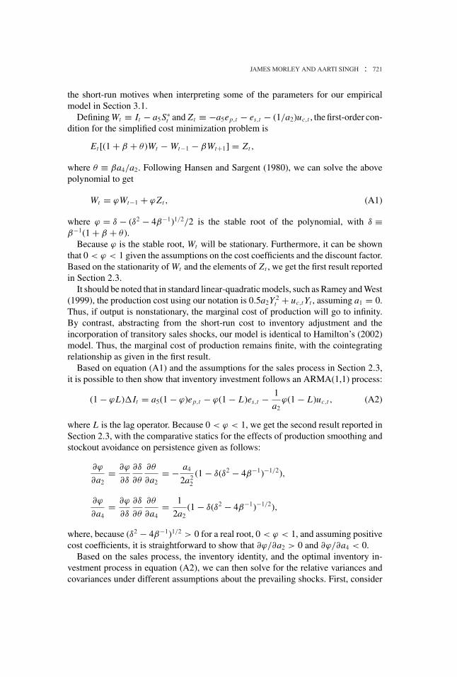
the short-run motives when interpreting some of the parameters for our empiricalmodel in Section 3.1.

Defining Wt ≡ It − a5S∗t and Zt ≡ −a5ep,t − es,t − (1/a2)uc,t , the first-order con-

dition for the simplified cost minimization problem is

Et [(1 + β + θ )Wt − Wt−1 − βWt+1] = Zt ,

where θ ≡ βa4/a2. Following Hansen and Sargent (1980), we can solve the abovepolynomial to get

Wt = ϕWt−1 + ϕZt , (A1)

where ϕ = δ − (δ2 − 4β−1)1/2/2 is the stable root of the polynomial, with δ ≡β−1(1 + β + θ ).

Because ϕ is the stable root, Wt will be stationary. Furthermore, it can be shownthat 0 < ϕ < 1 given the assumptions on the cost coefficients and the discount factor.Based on the stationarity of Wt and the elements of Zt , we get the first result reportedin Section 2.3.

It should be noted that in standard linear-quadratic models, such as Ramey and West(1999), the production cost using our notation is 0.5a2Y 2

t + uc,t Yt , assuming a1 = 0.Thus, if output is nonstationary, the marginal cost of production will go to infinity.By contrast, abstracting from the short-run cost to inventory adjustment and theincorporation of transitory sales shocks, our model is identical to Hamilton’s (2002)model. Thus, the marginal cost of production remains finite, with the cointegratingrelationship as given in the first result.

Based on equation (A1) and the assumptions for the sales process in Section 2.3,it is possible to then show that inventory investment follows an ARMA(1,1) process:

(1 − ϕL)�It = a5(1 − ϕ)ep,t − ϕ(1 − L)es,t − 1

a2ϕ(1 − L)uc,t , (A2)

where L is the lag operator. Because 0 < ϕ < 1, we get the second result reported inSection 2.3, with the comparative statics for the effects of production smoothing andstockout avoidance on persistence given as follows:

∂ϕ

∂a2= ∂ϕ

∂δ

∂δ

∂θ

∂θ

∂a2= − a4

2a22

(1 − δ(δ2 − 4β−1)−1/2),

∂ϕ

∂a4= ∂ϕ

∂δ

∂δ

∂θ

∂θ

∂a4= 1

2a2(1 − δ(δ2 − 4β−1)−1/2),

where, because (δ2 − 4β−1)1/2 > 0 for a real root, 0 < ϕ < 1, and assuming positivecost coefficients, it is straightforward to show that ∂ϕ/∂a2 > 0 and ∂ϕ/∂a4 < 0.

Based on the sales process, the inventory identity, and the optimal inventory in-vestment process in equation (A2), we can then solve for the relative variances andcovariances under different assumptions about the prevailing shocks. First, consider


only permanent sales shocks, setting the variances of the other shocks to zero. Thisimplies the following variance ratio and covariance expressions:

var(�Yt )

var(�St )= 1 + 2a5(1 − ϕ) + 2a2

5(1 − ϕ)2

1 + ϕ,

cov(�St ,�2 It )

var(�St )= a5(1 − ϕ).

It is straightforward to show that the variance ratio is strictly greater than one.Meanwhile, given that a5 > 0 and 0 < ϕ < 1, the covariance will be positive. Second,consider only transitory sales shocks, which implies the following expressions:

var(�Yt )

var(�St )= (1 − ϕ)2

1 + ϕ,

cov(�St ,�2 It )

var(�St )= ϕ(ϕ − 3)

2.

Again, given 0 < ϕ < 1, the variance ratio will be strictly less than one and thecovariance will be negative. Finally, consider only cost shocks, which implies thefollowing expressions:

var(�Yt )

var(uc,t )= 2ϕ2(3 − ϕ)

a22(1 + ϕ)

,

cov(�St ,�2 It ) = 0.

In this case, we cannot standardize by the variance of sales because it is zero. Butit is trivial to see that output will be more volatile than sales and the covariance ofinventories and sales will be zero. Taking all of these findings together, we get thethird result reported in Section 2.3.

Then, for the fourth and last result reported in Section 2.3, we can calculate thepartial effects of an unpredictable change in inventories on future output growth andfuture sales growth given a prevailing shock. To do this, we compute the ratio of themarginal effects of each shock on future output and sales growth and on inventories.First, consider a permanent sales shock:

∂�Yt+1

∂ep,t

/∂�It

∂ep,t= ϕ,

∂�St+1

∂ep,t

/∂�It

∂ep,t= 0.


Because 0 < ϕ < 1, inventory investment will have a positive relationship with futureoutput growth, whereas there is no relationship with future sales growth. Second,consider a transitory sales shock:

∂�Yt+1

∂es,t

/∂�It

∂es,t= 1 − ϕ + ϕ2

ϕ,

∂�St+1

∂es,t

/∂�It

∂es,t= 1

ϕ.

Again because 0 < ϕ < 1, it is straightforward to show that inventory investmentwill have a positive relationship with future output growth and future sales growth,with second expression greater than one and greater than the first expression—thatis, the effect on future sales growth is greater than the effect on future output growth.Finally, consider a cost shock:

∂�Yt+1

∂uc,t

/∂�It

∂uc,t= ϕ − 1,

∂�St+1

∂uc,t

/∂�It

∂uc,t= 0.

In this case, because 0 < ϕ < 1, inventory investment will have a negative relation-ship with future output growth, whereas there is no relationship with future salesgrowth.

APPENDIX B: STATE-SPACE REPRESENTATION

In this appendix, we present the state-space representation of the UC model inSection 3.1.

The observation equation isyt= H β t ,

where

yt =[

st

it

], H =

[1 0 0 0 1 00 0 1 0 1 1

]and β t =

⎡⎢⎢⎢⎢⎢⎢⎣

st − τ ∗t

st−1 − τ ∗t−1

it − i∗t

it−1 − i∗t−1

τ ∗tκt

⎤⎥⎥⎥⎥⎥⎥⎦.

The state equation is

β t = μ + Fβ t−1 + ν t ,


where

μ =

⎡⎢⎢⎢⎢⎢⎢⎢⎣

0000μτ

μκ

⎤⎥⎥⎥⎥⎥⎥⎥⎦, F =

⎡⎢⎢⎢⎢⎢⎢⎢⎣

φs,1 φs,2 0 0 0 01 0 0 0 0 00 0 φi,1 φi,2 0 00 0 1 0 0 00 0 0 0 1 00 0 0 0 0 1

⎤⎥⎥⎥⎥⎥⎥⎥⎦, ν t =

⎡⎢⎢⎢⎢⎢⎢⎢⎣

λsηηt + εt

0λiηηt + λiωωt + λiεεt + υt

0ηt

ωt + λκηηt

⎤⎥⎥⎥⎥⎥⎥⎥⎦,

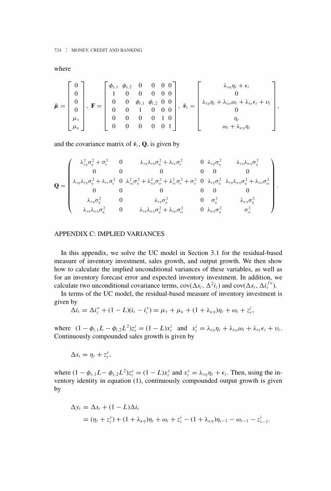
and the covariance matrix of ν t , Q, is given by

Q =

⎛⎜⎜⎜⎜⎜⎜⎜⎜⎜⎝

λ2sησ

2η + σ 2

ε 0 λsηλiησ2η + λiεσ

2ε 0 λsησ

2η λsηλκησ

2η

0 0 0 0 0 0

λsηλiησ2η + λiεσ

2ε 0 λ2

iησ2η + λ2

iωσ2ω + λ2

iεσ2ε + σ 2

υ 0 λiησ2η λiηλκησ

2η + λiωσ

2ω

0 0 0 0 0 0

λsησ2η 0 λiησ

2η 0 σ 2

η λκησ2η

λsηλκησ2η 0 λiηλκησ

2η + λiωσ

2ω 0 λκησ

2η σ 2

ω

⎞⎟⎟⎟⎟⎟⎟⎟⎟⎟⎠.

APPENDIX C: IMPLIED VARIANCES

In this appendix, we solve the UC model in Section 3.1 for the residual-basedmeasure of inventory investment, sales growth, and output growth. We then showhow to calculate the implied unconditional variances of these variables, as well asfor an inventory forecast error and expected inventory investment. In addition, wecalculate two unconditional covariance terms, cov(�st ,�

2it ) and cov(�st ,�i f et ).

In terms of the UC model, the residual-based measure of inventory investment isgiven by

�it = �i∗t + (1 − L)(it − i∗

t ) = μτ + μκ + (1 + λκη)ηt + ωt + zit ,

where (1 − φi,1L − φi,2L2)zit = (1 − L)xi

t and xit = λiηηt + λiωωt + λiεεt + υt .

Continuously compounded sales growth is given by

�st = ηt + zst ,

where (1 − φs,1 L− φs,2L2)zst = (1 − L)xs

t and xst = λsηηt + εt . Then, using the in-

ventory identity in equation (1), continuously compounded output growth is givenby

�yt = �st + (1 − L)�it

= (ηt + zst ) + (1 + λκη)ηt + ωt + zi

t − (1 + λκη)ηt−1 − ωt−1 − zit−1.


We can then write a vector representation for zst and zi

t as

zt = Kzt−1 + wt ,

where

zt =

⎡⎢⎢⎢⎢⎢⎢⎣

zst

zst−1zi

tzi

t−1xs

tx i

t

⎤⎥⎥⎥⎥⎥⎥⎦, K =

⎡⎢⎢⎢⎢⎢⎢⎣

φs,1 φs,2 0 0 −1 01 0 0 0 0 00 0 φi,1 φi,2 0 −10 0 1 0 0 00 0 0 0 0 00 0 0 0 0 0

⎤⎥⎥⎥⎥⎥⎥⎦, wt =

⎡⎢⎢⎢⎢⎢⎢⎣

xst

0xi

t0xs

tx i

t

⎤⎥⎥⎥⎥⎥⎥⎦.

Let W be the covariance matrix of wt , with the following nonzero entries: W[1, 1] =W[1, 5] = W[5, 1] = W[5, 5] = λ2

sησ2η + σ 2

ε , W[1, 3] = W[3, 1] = W[1, 6] =W[6, 1] = W[3, 5] = W[5, 3] = W[5, 6] = W[6, 5] = λsηλiησ

2η + λiεσ

2ε , and

W[3, 3] = W[3, 6] = W[6, 3] = W[6, 6] = λ2iησ

2η+λ2

iωσ2ω+λ2

iεσ2ε +σ 2

υ . Then,noting that vec(var(zt )) = (I − K ⊗ K)−1vec(W), the unconditional variance ofinventory investment is given by

var(�it ) = var((1 + λκη)ηt + ωt + zit )

= (1 + λκη)2σ 2η + σ 2

ω + var(zit ) + 2cov((1 + λκη)ηt , zi

t ) + 2cov(ωt , zit )

= (1 + λκη)2σ 2η + λ2

κεσ2ε + σ 2

ω + var(zit ) + 2(1 + λκη)λiησ

2η + 2λiωσ

2ω,

where var(zit ) is the [3, 3] element of var(zt ). The unconditional variances of the two

expectational components of inventory investment are given by

var(�i f et ) = (λyη − λsη)

2σ 2η + (λyε − 1)2σ 2

ε + λ2yωσ

2ω + σ 2

υ ,

and

var(�i et ) = var(�it ) − var(�i f e

t ).

The unconditional variance of sales growth is given by

var(�st ) = var(ηt + zst ) = σ 2

η + var(zst ) + 2λsησ

2η ,

where var(zst ) is the [1, 1] element of var(zt ), whereas the unconditional variance of

output growth is given by

var(�yt ) = var(�st +�it −�it−1) = var(�st ) + 2var(�it )

+ 2cov(�st ,�it ) − 2cov(�st ,�it−1) − 2cov(�it ,�it−1),


with

cov(�st ,�it ) = cov(ηt + zs

t , (1 + λκη)ηt + ωt + zit

)= (1 + λκη)σ

2η + (1 + λκη)λsησ

2η + cov

(zs

t , zit

) + λiησ2η ,

cov(�st ,�it−1) = cov(ηt + zs

t , (1 + λκη)ηt−1 + ωt−1 + zit−1

)= cov

(zs

t , zit−1

) + cov(zs

t , (1 + λκη)ηt−1 + ωt−1)

= cov(zs

t , zit−1

) + (φs,1 − 1)λsη(1 + λκη)σ2η ,

and

cov(�it ,�it−1) = cov((1 + λκη)ηt + ωt + zi

t , (1 + λκη)ηt−1 + ωt−1 + zit−1

)= cov

(zi

t , (1 + λκη)ηt−1 + ωt−1 + zit−1

)= (φi,1 − 1)

(λiη(1 + λκη)σ

2η + λiωσ

2ω

) + cov(zi

t , zit−1

),

where cov(zst , zi

t ), cov(zst , zi

t−1), and cov(zit , zi

t−1) are the [1, 3], [1, 4], and [3, 4]elements of var(zt ), respectively.

Finally, the two unconditional covariance terms are given by

cov(�st ,�i2

t

) = cov(ηt + zs

t , (1 + λκη)ηt + ωt + zit − (1 + λκη)ηt−1−ωt−1 − zi

t−1))

= cov(zs

t , zit−1

) + cov(zs

t , (1 + λκη)ηt−1 + ωt−1)

= (1 + λκη)σ2η + λiησ

2η + λsη(1 + λκη)σ

2η − (φs,1−1)λsη(1 + λκη)σ

2η

+ cov(zs

t , zit

) − cov(zs

t , zit−1

),

and

cov(�st ,�i f et ) = cov(ηt + zs

t , (λyη − λsη)ηt + (λyε − 1)εt + λyωωt + υt )

= (λyη − λsη)σ2η + (λyε − 1)σ 2

ε + λsη(λyη − λsη)σ2η .

LITERATURE CITED

Ahmed, Shaghil, Andrew Levin, and Beth A. Wilson. (2004) “Recent U.S. MacroeconomicStability: Good Luck, Good Policies, or Good Practices?” Review of Economics and Statis-tics, 86, 824–32.

Blanchard, Olivier J. (1983) “The Production and Inventory Behavior of the American Auto-mobile Industry.” Journal of Political Economy, 91, 585–614.

Blinder, Alan S., and Louis J. Maccini. (1991) “Taking Stock: A Critical Assessment of theRecent Research on Inventories.” Journal of Economic Perspectives, 5, 73–96.


Camacho, Maximo, Gabriel Perez-Quiros, and Hugo R. Mendizabal. (2011) “High-GrowthRecoveries, Inventories and the Great Moderation.” Journal of Economic Dynamics andControl, 35, 1322–39.

Chib, Siddhartha, and Edward Greenberg. (1995) “Understanding the Metropolis-HastingsAlgorithm.” American Statistician, 49, 327–35.

Clarida, Richard H., Jordi Gali, and Mark L. Gertler. (2000) “Monetary Policy Rules andMacroeconomic Stability: Evidence and Some Theory.” Quarterly Journal of Economics,115, 147–80.

Clark, Todd E. (2009) “Is the Great Moderation Over? An Empirical Analysis.” FederalReserve Bank of Kansas City Economic Review, 4, 5–42.

Davis, Steven J., and James A. Kahn. (2008) “Interpreting the Great Moderation: Changes inthe Volatility of Economic Activity at the Macro and Micro Levels.” Journal of EconomicPerspectives, 22, 155–80.

Eo, Yunjong, and James C. Morley. (2015) “Likelihood-Ratio-Based Confidence Sets for theTiming of Structural Breaks.” Quantitative Economics, 6, 463–97.

Golob, John E. (2000) “Post-1984 Inventories Revitalize the Production Smoothing Model.”Mimeo.

Granger, Clive W. J., and Tae H. Lee. (1989) “Investigation of Production, Sales and InventoryRelationships Using Multicointegration and Non-Symmetric Error Correction Models.”Journal of Applied Econometrics, 4, S145–S159.

Hamilton, James D. (2002) “On the Interpretation of Cointegration in the Linear-QuadraticInventory Model.” Journal of Economic Dynamics and Control, 26, 2037–49.

Hansen, Lars P., and Thomas J. Sargent. (1980) “Formulating and Estimating Dynamic LinearRational Expectations Model.” Journal of Economic Dynamics and Control, 2, 7–46.

Herrera, Ana M., Irina Murtazashvili, and Elena Pesavento. (2008) “The Comovement inInventories and in Sales: Higher and Higher.” Economics Letters, 99, 155–8.

Herrera, Ana M., and Elena Pesavento. (2005) “The Decline in U.S. Output Volatility: Struc-tural Changes and Inventory Investment.” Journal of Business & Economic Statistics, 23,462–72.

Holt, Charles C., Franco Modigliani, John F. Muth, and Herbert A. Simon. (1960) PlanningProduction, Inventories, and Work Force. Englewood Cliffs, NJ: Prentice Hall.

Irvine, Owen F., and Scott Schuh. (2005) “The Roles of Comovement and Inventory Investmentin the Reduction of Output Volatility.” Federal Reserve Bank of Boston, Research PaperSeries, Working Paper No. 05–9.

Kahn, James A., Margaret M. McConnell, and Gabriel Perez-Quiros. (2002) “On the Causesof the Increased Stability of the U.S. Economy.” FRBNY Economic Policy Review, 8,183–202.

Kim, Chang-Jin, James C. Morley, and Jeremy Piger. (2008) “Bayesian Counterfactual Anal-ysis of the Sources of the Great Moderation.” Journal of Applied Econometrics, 23, 173–91.

Kim, Chang-Jin, and Charles R. Nelson. (1999) “Has the U.S. Economy Become More Stable?A Bayesian Approach Based on a Markov-Switching Model of the Business Cycle.” Reviewof Economics and Statistics, 81, 608–16.

Maccini, Louis J., Bartholomew Moore, and Huntley Schaller. (2015) “Inventory Behav-ior with Permanent Sales Shocks.” Journal of Economic Dynamics and Control, 53,290–313.


Maccini, Louis J., and Adrian Pagan. (2013) “Inventories, Fluctuations, and Goods SectorCycles.” Macroeconomic Dynamics, 17, 89–122.

McCarthy, Jonathan, and Egon Zakrajsek. (2007) “Inventory Dynamics and Business Cycles:What Has Changed?” Journal of Money, Credit and Banking, 39, 615–38.

McConnell, Margaret M., Patricia C. Mosser, and Gabriel Perez-Quiros. (1999) “A Decom-position of the Increased Stability of GDP Growth.” FRBNY Current Issues in Economicsand Finance, 5, 1–6.

McConnell, Margaret M., and Gabriel Perez-Quiros. (2000) “Output Fluctuations in the UnitedStates: What Has Changed Since the Early 1980s?” American Economic Review, 90, 1464–76.

Miron, Jeffrey A., and Stephen P. Zeldes. (1988) “Seasonality, Cost Shocks, and the ProductionSmoothing Model of Inventories.” Econometrica, 56, 877–908.

Morley, James C. (2007) “The Slow Adjustment of Aggregate Consumption to PermanentIncome.” Journal of Money, Credit and Banking, 39, 615–38.

Morley, James C., Charles R. Nelson, and Eric Zivot. (2003) “Why Are the Beveridge-Nelsonand Unobserved-Component Decompositions of GDP so Different?” Review of Economicsand Statistics, 85, 235–43.

Ramey, Valerie A., and Daniel J. Vine. (2004) “Why Do Real and Nominal Inventory-SalesRatios Have Different Trends?” Journal of Money, Credit and Banking, 36, 959–63.

Ramey, Valerie A., and Kenneth D. West. (1999) “Inventories.” In Handbook of Macroeco-nomics, edited by John B. Taylor and Michael Woodford, pp. 863–923. New York: NorthHolland, Elsevier.

Sims, Christopher A., and Tao Zha. (2006) “Were There Regime Switches in US MonetaryPolicy?” American Economic Review, 96, 54–81.

Sinclair, Tara. (2009) “The Relationship between Permanent and Transitory Movements inU.S. Output and the Unemployment Rate.” Journal of Money Credit and Banking, 41,529–42.

Stock, James, and Mark Watson. (2003) “Has the Business Cycle Changed and Why?” NBERMacroeconomics Annual 2002, 17, 159–218.

Wen, Yi. (2005) “Understanding the Inventory Cycle.” Journal of Monetary Economics, 52,1533–55.

West, Kenneth D. (1986) “A Variance Bounds Test of the Linear Quadratic Inventory Model.”Journal of Political Economy, 94, 374–401.

West, Kenneth D. (1990) “The Sources of Fluctuations in Aggregate Inventories and GNP.”Quarterly Journal of Economics, 105, 939–72.

Inventory Shocks and the Great Moderationresearch.economics.unsw.edu.au/jmorley/ms16.pdfThese...

Documents

Transcript of Inventory Shocks and the Great Moderationresearch.economics.unsw.edu.au/jmorley/ms16.pdfThese...