Inventory Management Models
15
CHAPTER 2: INVENTORY MANAGEMENT AND RISK POOLING 33 6. Service level requirements. In situations where customer demand is uncertain, it is often impossible to meet customer orders 100 percent of the time, so management needs to specify an acceptable level of service. 2.2 SINGLE STAGE INVENTORY CONTROL We start by considering inventory management in a single supply chain stage. There are a variety of techniques and approaches that can be effective for managing inventory in a single stage, depending on the characteristics of that stage. 2.2.1 The Economic Lot Size Model The classic economic lot size model, introduced by Ford W. Harris in 1915, is a simple model that illustrates the trade-offs between ordering and storage costs. Consider a warehouse facing constant demand for a single item. The warehouse orders from the supplier, who is assumed to have an unlimited quantity of the product. The model assumes the following: • Demand is constant at a rate of D items per day. • Order quantities are fixed at Q items per order; that is, each time the warehouse places an order, it is for Q items. • A fixed cost (setup cost), K, is incurred every time the warehouse places an order. • An inventory carrying cost, h, also referred to as a holding cost, is accrued per unit held in inventory per day that the unit is held. • The lead time, the time that elapses between the placement of an order and its receipt, is zero. • Initial inventory is zero. • The planning horizon is long (infinite). Our goal is to find the optimal order policy that minimizes annual purchasing and carrying costs while meeting all demand (that is, without shortage). This is an extremely simplified version of a real inventory system. The assumption of a known fixed demand over a long horizon is clearly unrealistic. Replenishment of products very likely takes several days, and the requirement of a fixed order quantity is restrictive. Surprisingly, the insight derived from this model will help us to develop inventory policies that are effective for more complex realistic systems. It is easy to see that in an optimal policy for the model described above, orders should be received at the warehouse precisely when the inventory level drops to zero. This is called the zero inventory ordering property, which can be observed by con- sidering a policy in which orders are placed and received when the inventory level is not zero. Clearly, a cheaper policy would involve waiting until the inventory is zero before ordering, thus saving on holding costs. To find the optimal ordering policy in the economic lot size model, we consider the inventory level as a function of time; see Figure 2-3. This is the so-called saw-toothed inventory pattern. We refer to the time between two successive replenishments as a cycle time. Thus, total inventory cost in a cycle of length Tis K + hTQ 2 since the fixed cost is charged once per order and holding cost can be viewed as the product of the per-unit, per-time-period holding cost, h; the average inventory level, Q/2; and the length of the cycle, T.
Transcript of Inventory Management Models

CHAPTER 2 INVENTORY MANAGEMENT AND RISK POOLING 33
6 Service level requirements In situations where customer demand is uncertain it is often impossible to meet customer orders 100 percent of the time so management needs to specify an acceptable level of service
22 SINGLE STAGE INVENTORY CONTROL
We start by considering inventory management in a single supply chain stage There are a variety of techniques and approaches that can be effective for managing inventory in a single stage depending on the characteristics of that stage
221 The Economic Lot Size Model
The classic economic lot size model introduced by Ford W Harris in 1915 is a simple model that illustrates the trade-offs between ordering and storage costs Consider a warehouse facing constant demand for a single item The warehouse orders from the supplier who is assumed to have an unlimited quantity of the product The model assumes the following
bull Demand is constant at a rate of D items per day bull Order quantities are fixed at Q items per order that is each time the warehouse
places an order it is for Q items bull A fixed cost (setup cost) K is incurred every time the warehouse places an order bull An inventory carrying cost h also referred to as a holding cost is accrued per unit
held in inventory per day that the unit is held bull The lead time the time that elapses between the placement of an order and its
receipt is zero bull Initial inventory is zero bull The planning horizon is long (infinite)
Our goal is to find the optimal order policy that minimizes annual purchasing and carrying costs while meeting all demand (that is without shortage)
This is an extremely simplified version of a real inventory system The assumption of a known fixed demand over a long horizon is clearly unrealistic Replenishment of products very likely takes several days and the requirement of a fixed order quantity is restrictive Surprisingly the insight derived from this model will help us to develop inventory policies that are effective for more complex realistic systems
It is easy to see that in an optimal policy for the model described above orders should be received at the warehouse precisely when the inventory level drops to zero This is called the zero inventory ordering property which can be observed by conshysidering a policy in which orders are placed and received when the inventory level is not zero Clearly a cheaper policy would involve waiting until the inventory is zero before ordering thus saving on holding costs
To find the optimal ordering policy in the economic lot size model we consider the inventory level as a function of time see Figure 2-3 This is the so-called saw-toothed inventory pattern We refer to the time between two successive replenishments as a cycle time Thus total inventory cost in a cycle of length Tis
K + hTQ 2
since the fixed cost is charged once per order and holding cost can be viewed as the product of the per-unit per-time-period holding cost h the average inventory level Q2 and the length of the cycle T
34 DESIGNING AND MANAGING THE SUPPLY CHAIN
Order size
Time
FIGURE 2-3 Inventory level as a function of time
Since the inventory level changes from Qto 0 during a cycle of length T and demand is constant at a rate ofD units per unit time it must be that Q = TD Thus we can divide the cost above by T or equivalently QD to get the average total cost per unit of time
KD hQ Q+T
Using simple calculus it is easy to show that the order quantity Q that minimizes the cost function above is
Q = vYfP The simple model provides two important insights
1 An optimal policy balances inventory holding cost per unit time with setup cost per unit time Indeed setup cost per unit time = KD Q while holding cost per unit time = hQ2 (see Figure 2-4) Thus as one increases the order quantity Q inventory holding costs per unit of time increase while setup costs per unit of time decrease The optimal order quantity is achieved at the point at which inventory setup cost per unit of time (KD Q ) equals inventory holding cost per unit of time (hQ2) That is
KD hQ
Q 2 or
Q = vYfP $160
$140
$120
$100 0 $80U
$60
$40
$20
$0 0 500 1000 1500
Order quantity (number of units)
FIGURE 2-4 Economic lot size model total cost per unit time
Holding cost
CHAPTER 2 INVENTORY MANAGEMENT AND RISK POOLING 35
2 Total inventory cost is insensitive to order quantities that is changes in order quantities have a relatively small impact on annual setup costs and inventory holding costs To illustrate this issue consider a decision maker that places an order quantity Q that is a multiple b of the optimal order quantity Q In other words for a given b the quantity ordered is Q = bQ Thus b = 1 implies that the decision maker orders the economic order quantity If b = 12 (b = 08) the decision maker orders 20 percent more (less) than the optimal order quantity Table 2-1 presents the impact of changes in b on total system cost For example if the decision maker orders 20 percent more than the optimal order quantity (b = 12) then the increase in total inventory cost relative to the optimal total cost is no more than 16 percent
TABLE 2-1
SENSITIVITY ANALYSIS
b Increase in cost
05 25
08 25
09 05 o
11 04
12 16
15 89
2 25
EXAMPLE 2middot2
Considera hardware supplywarehou~ethat is contractually obligated JOOO units of a specializ~fa$tEm~ I~cal manufacturing (ie)miflarw~~abl time the wareh~~e placesanor~ ms from its SUI)PllefFsn In~Inrtti(n fee of $Js charged to t e warehouse charges the loca~bull $500 fO(~ holding cost is or $025 per yeari~~
to know how gets to zeroilt demand (aSSuming~
1lltbull~IIU~1 holding cost is $o2~~r ehlJlolaCE~s an order the op~~1
222 The Effect of Demand Uncertainty
The previous model illustrates the trade-offs between setup costs and inventory holding costs It ignores however issues such as demand uncertainty and forecasting Indeed many companies treat the world as if it were predictable making production and inventory decisions based on forecasts of the demand made far in advance of the selling season Although these companies are aware of demand uncertainty when they create a forecast they design their planning processes as if the initial forecast was an accurate representation of reality In this case one needs to remember the following principles of all forecasts (see [148])
1 The forecast is always wrong 2 The longer the forecast horizon the worse the forecast 3 Aggregate forecasts are more accurate
Thus the first principle implies that it is difficult to match supply and demand and the second one implies that it is even more difficult if one needs to predict customer demand for a long period of time for example the next 12 to 18 months The third
36 DESIGNING AND MANAGING THE SUPPLY CHAIN
principle suggests for instance that while it is difficult to predict customer demand for individual SKUs it is much easier to predict demand across all SKUs within one product family This principle is an example of the risk pooling concept (see Section 23)
223 Single Period Models
To better understand the impact of demand uncertainty we consider a series of increasingly detailed and complex situations To start we consider a product that has a short lifecycle and hence the firm has only one ordering opportunity Thus before demand occurs the firm must decide how much to stock in order to meet demand If the firm stocks too much it will be stuck with excess inventory it has to dispose of If the firm stocks too little it will forgo some sales and thus some profits
Using historical data the firm can typically identify a variety of demand scenarios and determine a likelihood or probability that each of these scenarios will occur Observe that given a specific inventory policy the firm can determine the profit associated with a particular scenario Thus given a specific order quantity the firm can weight each scenarios profit by the likelihood that it will occur and hence determine the average or expected profit for a particular ordering quantity It is thus natural for the firm to order the quantity that maximizes the average profit
EXAMPLE 2-3
FIGURE 2middot5 ~forecast
CHAPTER 2 INVENTORY MANAGEMENT AND RISK POOLING 37
Interestingly the order quantity that maximizes total expected profit is not necshyessarily equal to the average demand Indeed in the previous example the order quantity that maximizes total expected profit is 12000 units while average demand is 13000
38 DESIGNING AND MANAGING THE SUPPLY CHAIN
So what is the relationship between the optimal order or production quantity and average demand Should the optimal order quantity always be less than average demand as in the previous example To answer these questions we compare the marginal profit and the marginal cost of ordering an additional unit If an additional unit is sold the marginal profit is the difference between the selling price per unit and the variable ordering (or production) cost per unit and if an additional unit is not sold during the selling season the marginal cost is the difshyference between the variable production cost and the salvage value per unit If the cost of not selling an additional unit is larger than the profit from selling an additional unit the optimal quantity in general will be less than average demand while if the reverse is true the optimal order quantity in general will be greater than the average demand
EXAMPLE 2-4
Lets ramptlli~ritamp()~rEl~~lln thise~lttrnple ave~~i~tS060unitswe sawprevioJ~f9i that the optimal order quantity is around 12000 units Why is this the case
For this purpose evaluat$the marginal profit and the marginal cost of producing an additional swimsuit If this swimsuit is soldduri~thEi su~mer season then the marginal profIt (sequal to $45 If the additional swimsuit is not sold during the summer season the margirujlcost is equal to $60 Thus the cost of not selling this additional sWimsuit during the summer season is larger than the profit obtained from selling itduringtrye seas()lllnd hence the optimal production quantity is less than the average demand
bull
Of course this is only true if minimizing average profit is in fact the goal of the firm As with other types of investments investment in inventory carries downside risks if sales do not meet expectations and upside rewards if demand exceeds expectations Interestingly it is possible to characterize the upside potential and downside risks in our model and thus assist management in inventory investment decisions
EXAMPLE 2-5
Once again consider the prEivi~usElXample Fi~re 2-6 plots the avera~prof~aslilflJnction of the production quantity As mentlohedatgtOye it shoWs that the optimal productlonquantitythat is the quantity that maximizes profltisatx)ut12000 The figure also indicates thatproducing 9000 units or unitswill teadfOCibout the same aver~gepro~itof$294OOOIfW
between prod t 16000 units whicllone
associated with cert~in construct a freq Figure 2-7) that pro~~es for the two giv 9000 units and 1~(1QO
profit when the pro notsymmeti~al Lo
t6OOO units The graph sIiOVl$ $2200d0 happen about 11 pe~nt of the
time while profits of at least $410000~appen50 percent of the time Onttle otherhand a fraqueocyenqistog~~pfttle profit when theprodUc~nqll~nfity~q90units shows that the isshytributiontIa~ltIpmiddot pltgt~slble outcomes Profitseit~~~()O_~ith probability of abollf11 percentQ(~ Witlto0bability of about 89 p~r~Q~toy~wheprodUcing 16000 units has the same~vefigeprofjta$producing 9000 unitsilt1I1tl~~IISko(l1he one hand and possible rewaraontheQtherhandincreases as we jncrea~~pr6(lu9tlt)nsize
CHAPTER 2 INVENTORY MANAGEMENT AND RISK POOLING 39
EXAMPLE a-sltfftfnued
100 ---~~--~--~------------
80 ~----------~--~N---------~
-2 60 ~Q=9OOOg
0 0 40 bull Q= 16(OO ~
20
(in thousltmd~l ~ bull
To summarize
bull The optimal order quantity is not necessarily equal to forecast or average demand Indeed the optimal quantity depends on the relationship between marginal profit achieved from selling an additional unit and marginal cost More importantly the fixed cost has no impact on the production quantity only on the decision whether to produce or not Thus given a decision to produce the production quantity is the same independently of the fixed production cost
bull As the order quantity increases average profit typically increases until the proshyduction quantity reaches a certain value after which the average profit starts decreasing
bull As we increase the production quantity the risk--that is the probability of large losses--always increases At the same time the probability of large gains also increases This is the riskreward trade-off
224 Initial Inventory
In the previous model we considered a situation in which the firm has only a single ordering or production opportunity to meet demand during a short selling season We next consider a similar situation but one in which the firm already has some inventory of the product on hand perhaps inventory left over from the previous season If no additional order is placed or produced the on-hand inventory can be used to meet demand but of course the firm cannot sell more than this initial inventory level On the other hand if an order is placed the fixed cost must be paid and additional inventory can be acquired Thus when initial inventory is available the trade-off is between having a limited amount of inventory by avoiding paying the fixed cost versus paying the fixed cost and therefore having a higher inventory level
EXAMPLE 2-6
Recall ourpteifl)U$exall1pt~and suppose now thaH~~iTt~llit lJh~rconsideration is a moder producecj ISEtY$arand1hatthe manufacturer has arrill(ti~J itlVernoryQf 5000 units Assuming t~at demand for this modamplfollowS the same pattern of scenarios asbefQre should the manufacturer start production and if$Ot)()w many swimsuits shoQl~be proquced
40 DESIGNING AND MANAGING THE SUPPLY CHAIN
The previous example motivates a powerful inventory policy used in practice to manage inventory Whenever the inventory level is reviewed if it is below a certain value say s we order (or produce) to increase the inventory to level S Such a policy is referred as an (s S ) policy or a min max policy We typically refer to s as the reorder point or the min and to S as the order-up-to level or the max Finally observe that if
CHAPTER 2 INVENTORY MANAGEMENT AND RISK POOLING 41
there is no fixed cost the optimal inventory is characterized by a single number the order-up-to level always order enough to raise inventory ta the target inventory level
EXAMPLE 2-7
In the swimsuit production example the reorder point is 8500 units and the order-up-tolevel is 12000 units The difference between these two levels is driven by fixed costs associated with ordering manufacturing or transportation
225 Multiple Order Opportunities
The situations we considered above all focus on a single ordering or production opportunity This may be the case for fashion items where the selling season is short and there is no second opportunity to reorder products based on realized customer demand In many practical situations however the decision maker may order products repeatedly at any time during the year
Consider for instance a distributor that faces random demand for a product and meets that demand with product ordered from a manufacturer Of course the manushyfacturer cannot instantaneously satisfy orders placed by the distributor there is a fixed lead time for delivery whenever the distributor places an order Since demand is random and the manufacturer has a fixed delivery lead time the distributor needs to hold inventory even if no fixed setup cost is charged for ordeling the products There are at least three reasons why the distributor holds inventory
1 To satisfy demand occurring during lead time Since orders arent met immeshydiately inventory must be on hand to meet customer demand that is realized between the time that the distributor places an order and the time that the ordered inventory arrives
2 To protect against uncertainty in demand 3 To balance annual inventory holding costs and annual fixed order costs We have
seen that more frequent orders lead to lower inventory levels and thus lower inventory holding costs but they also lead to higher annual fixed order costs
While these issues are intuitively clear the specific inventory policy that the disshytributor should apply is not simple To manage inventory effectively the distributor needs to decide when and how much to order We distinguish between two types of policies
bull Continuous review policy in which inventory is reviewed continuously and an order is placed when the inventory reaches a particular level or reorder point This type of policy is most appropriate when inventory can be continuously reviewedshyfor example when computerized inventory systems are used
bull Periodic review policy in which the inventory level is reviewed at regular intervals and an appropriate quantity is ordered after each review This type of policy is most appropriate for systems in which it is impossible or inconvenient to frequently review inventory and place orders if necessary
226 Continuous Review Policy
We first consider a system in which inventory is continuously reviewed Such a review system typically provides a more responsive inventory management strategy than the one associated with a periodic review system (why)
42 DESIGNING AND MANAGING THE SUPPLY CHAIN
We make the following additional assumptions
bull Daily demand is random and follows a normal distribution In other words we assume that the probabilistic forecast of daily demand follows the famous bell-shaped curve Note that we can completely describe normal demand by its average and standard deviation
bull Every time the distributor places an order from the manufacturer the distributor pays a fixed cost K plus an amount proportional to the quantity ordered
bull Inventory holding cost is charged per item per unit time bull Inventory level is continuously reviewed and if an order is placed the order arrives
after the appropriate lead time bull If a customer order arrives when there is no inventory on hand to fill the order (ie
when the distributor is stocked out) the order is lost bull The distributor specifies a required service level The service level is the probability
of not stocking out during lead time For example the distributor might want to ensure that the proportion of lead times in which demand is met out of stock is 95 percent Thus the required service level is 95 percent in this case
To characterize the inventory policy that the distributor should use we need the following information
AVG = Average daily demand faced by the distributor STD = Standard deviation of daily demand faced by the distributor L = Replenishment lead time from the supplier to the distributor in days h = Cost of holding one unit of the product for one day at the distributor a = service level This implies that the probability of stocking out is 1 - a
In addition we need to define the concept of inventory position The inventory position at any point in time is the actual inventory at the warehouse plus items ordered by the distributor that have not yet arrived minus items that are backordered
To describe the policy that the distributor should use we recall the intuition developed when we considered a single period inventory model with initial inventory In that model when inventory was below a certain level we ordered enough to raise the inventory up to another higher level For the continuous review model we employ a similar approach known as a (Q R) policy-whenever inventory level falls to a reorder level R place an order for Q units
The reorder level R consists of two components The first is the average inventory during lead time which is the product of average daily demand and the lead time This ensures that when the distributor places an order the system has enough inventory to cover expected demand during lead time The average demand during lead time is exactly
LXAVG
The second component represents the safety stock which is the amount of inventory that the distributor needs to keep at the warehouse and in the pipeline to protect against deviations from average demand during lead time This quantity is calculated as follows
z X STD X Vi where z is a constant referred to as the safety factor This constant is associated with the service level Thus the reorder level is equal to
L X AVG + z X STD X Vi
CHAPTER 2 INVENTORY MANAGEMENT AND RISK POOLING 43
TABLE 2-2
SERVICE LEVEL AND THE SERVICE FACTOR Z
Service level 90 91 92 93 94 95 96 97 98 99 999 z 129 134 141 148 156 165 1 75 188 205 233 308
The safety factor z is chosen from statistical tables to ensure that the probability of stockouts during lead time is exactly I - lY This implies that the reorder level must satisfy
PrDemand during lead time 2 LX AVG + z X STD X vL = 1 - lY
Table 2-2 provides a list of z values for different values of the service level lY
What about the order quantity Q Although calculating the optimal Q for this model is not easy the EOQ order quantity we developed previously is very effective for this model Recall from this model that the order quantity Q is calculated as follows
Q = V2K Xz AVG
If there is no variability in customer demand the distributor would order Q items when the inventory is at level L X AVG since it takes L days to receive the order However there is variability in demand so the distributor places an order for Q items whenever the inventory position is at the reorder level R
Figure 2-9 illustrates the inventory level over time when this type of policy is implemented What is the average inventory level in this policy Observe that between two successive orders the minimum level of inventory is achieved right before receiving an order while the maximum level of inventory is achieved immeshydiately after receiving the order The expected level of inventory before receiving the order is the safety stock
z X STD X vL while the expected level of inventory immediately after receiving the order is
Q + z X STD X vL Thus the average inventory level is the average of these two values which is equal to
+ z X STD X vL
Q + R ----------------------------shy
~ Inventory position
Inventory level
R--------~~L---_+------~-----
Lead time
o----------------------~~
Time_
FIGURE 2-9 Inventory level as a function of time in a (Q R) policy
44 DESIGNING AND MANAGING THE SUPPLY CHAIN
EXAMPLE 2-8
Consider a distributor of TV sets~~~order$fbnla manufacturer and dislritlutor of the TV sets is )Iinglo set invntory policies at the wat~~Ulsjl1f~iilSl mod~ Assume that when~rtnedistribJt~mplaces an order for TV Seamplt~l~~i~middotfixl~dol1Jlerilng cost Of $4500 which is indepe~lltofthe~~rsizeThe cost of a TV and annual inventory holding costfsabout18percent of the product cmlt~1ePile leacUime) is about two weeks
Table 2-3 provides data Given that the distributor WUI~middotK~
the otijer
CHAPTER 2 INVENTORY MANAGEMENT AND RISK POOLING 45
227 Variable Lead Times
In many cases the assumption that the delivery lead time to the warehouse is fixed and known in advance does not necessarily hold Indeed in many practical situations the lead time to the warehouse may be random or unknown in advance In these cases we typically assume that the lead time is normally distributed with average lead time denoted by AVGL and standard deviation denoted by STDL In this case the reorder point R is calculated as follows
R = AVG X AVGL + zYAVGL X STD2 + AVG2 X STDL2
where AVG X AVGL represents average demand during lead time while
YAVGL X STD2 + A VG2 X STDL2
is the standard deviation of demand during lead time Thus the amount of safety stock that has to be kept is equal to
zYAVGL X STD2 + AVG2 X STDL2
As before the order quantity Q satisfies Q = y2K xh AVG
228 Periodic Review Policy
In many real-life situations the inventory level is reviewed periodically at regular intervals and an appropriate quantity is ordered after each review If these intervals are relatively short (for example daily) it may make sense to use a modified version of the (Q R) policy presented above Unfortunately the (Q R) policy cant be directly implemented since the inventory level may fall below the reorder point when the warehouse places an order To overcome this problem define two inventory levels s and S and during each inventory review if the inventory position falls below s order enough to raise the inventory position to S We call this modified (Q R) policy an (s S) policy Although it is difficult to determine the optimal values for sand S one very effective approximation is to calculate the Q and R values as if this were a conshytinuous review model set s equal to R and S equal to R + Q
If there is a larger time between successive reviews of inventory (weekly or monthly for example) it may make sense to always order after an inventory level review Since an order is placed after each inventory review the fixed cost of placing an order is a sunk cost and hence can be ignored presumably the fixed cost was used to determine the review interval The quantity ordered arrives after the appropriate lead time
What inventory policy should the warehouse use in this case Since fixed cost does not playa role in this environment the inventory policy is characterized by a single parameter the base-stock level That is the warehouse determines a target inventory level the base-stock level and each review period the inventory position is reviewed and the warehouse orders enough to raise the inventory position to the base-stock level
What is an effective base-stock level For this purpose let r be the length of the review period-we assume that orders are placed every r periods of time As before L is the lead time AVG is the average daily demand faced by the warehouse and STD is the standard deviation of this daily demand
Observe that at the time the warehouse places an order this order raises the inventory position to the base-stock level This level of the inventory position should be enough to protect the warehouse against shortages until the next order arrives Since the next order arrives after a period of r + L days the current order should be enough to cover demand during a period of r + L days
46 DESIGNING AND MANAGING THE SUPPLY CHAIN
L L L
t Base-stock Level bull
aJ shyOJ
l gt ~ OJshy
s 0 -Time
FIGURE 2-10 Inventory level as a function of time in a periodic review policy
Thus the base-stock level should include two components average demand during an interval of r + L days which is equal to
(r + L) X AVG
and the safety stock which is the amount of inventory that the warehouse needs to keep to protect against deviations from average demand during a period of r + L days This quantity is calculated as follows
z X STD X v---+L where z is the safety factor
Figure 2-10 illustrates the inventory level over time when this type of policy is implemented What is the average inventory level in this case As before the maximum inventory level is achieved immediately after receiving an order while the minimum level of inventory is achieved just before receiving an order It is easy to see that the expected level of inventory after receiving an order is equal to
r X AVG + z X STD X v---+L while the expected level of inventory before an order arrives is just the safety stock
z X STD X v---+L Hence the average inventory level is the average of these two values which is equal to
r X t VGr X STD X v---+L
EXAMPLE 2-9
We cQOtinu~middotwith th~PI~viPusexan1pl~nd ass~~tlat the~~orplai~Qorder folttsets every three weeks Since lead time is twoweeks the base-stock level needs to cover a period of five weeks Thusaverage deilland during that period is
4458 xc5middot~2229 gt- -
and the~f~ty stoCk~~(~7 per~~~ice le~ls 19 X 328 x IS = 139
Hencethebase-stoc~levelshOulgpef23 + 13()==359Thatis~hen th~distributor pJilces an order~efyenthree WeEf~r he Shoul4~~aise thei~~ntory po$iti~nto 359Wlt_s TheillveJ11ge inventorY -middot1eVe1 in thi$~~equals -~~lt Mt ~lt - -(
ax5819X3208 x IS = 20a17
which implif9s that 0fI average thedistributor keepl3five (= 2Q1Y4458) w~ of suPply
CHAPTER 2 INVENTORY MANAGEMENT AND RISK POOLING 47
229 Service Level Optimization
So far we have assumed that the objective of this inventory optimization is to determine the optimal inventory policy given a specific service level target The question of course is how the facility should decide on the appropriate level of service Sometimes this is determined by the downstream customer In other words the retailer can require the facility for example the supplier to maintain a specific level of service and the supplier will use that target to manage its own inventory
In other cases the facility has the flexibility to choose the appropriate level of service The trades-offs presented in Figure 2-11 are clear everything else being equal the higher the service level the higher the inventory level Similarly for the same inventory level the longer the lead time to the facility the lower the level of service provided by the facility Finally the marginal impact on service level decreases with inventory level That is the lower the inventory level the higher the impact of a unit of inventory on service level and hence on expected profit
Thus one possible strategy used in retailing to determine service level for each SKU is to focus on maximizing expected profit across all or some of their products That is given a target service level across all products we determine service level for each SKU so as to maximize expected profit Everything else being equal service level will be higher for products with
bull High profit margin bull High volume bull Low variability bull Short lead time
10000
shy
9900
I
9800
I I
I I9700
I I
OJ 9600 I
OJ Igt
l
II
OJ 9500
Eu IOJ
() 9400 I I
I
9300
I 9200
I I I9100 I9000
390 440 490 540
Inventory
1--Lead time = 2 - - - - _ Lead time = 4 1 FIGURE 2middot11 Service level versus inventory level as a function of lead time
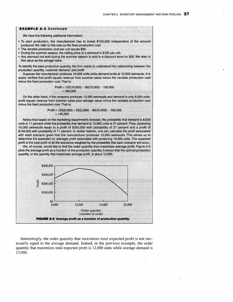


![An inventory model for optimal cash management …...size" model of inventory management [2]. A number of inventory theoretic models have also appeared for cash management problems](https://static.fdocuments.net/doc/165x107/5e98907f7adb6c45dc6d6486/an-inventory-model-for-optimal-cash-management-size-model-of-inventory.jpg)