This article was downloaded by: [AAG ]On: 22 March 2013, At: 10:14Publisher: RoutledgeInforma Ltd Registered in England and Wales Registered Number: 1072954Registered office: Mortimer House, 37-41 Mortimer Street, London W1T 3JH,UK

The Professional GeographerPublication details, including instructions forauthors and subscription information:http://www.tandfonline.com/loi/rtpg20

Invasive Saltcedar (Tamariskspp.) Distribution MappingUsing Multiresolution RemoteSensing ImageryLe Wang a , José L. Silván-Cárdenas b , Jun Yang c &Amy E. Frazier da Beijing Normal Universityb Centro de Investigación en Geografía y Geomática“Ing. Jorge L. Tamayo”c Beijing Forestry Universityd State University of New York–BuffaloVersion of record first published: 21 May 2012.

To cite this article: Le Wang , José L. Silván-Cárdenas , Jun Yang & Amy E. Frazier(2013): Invasive Saltcedar (Tamarisk spp.) Distribution Mapping Using MultiresolutionRemote Sensing Imagery, The Professional Geographer, 65:1, 1-15

To link to this article: http://dx.doi.org/10.1080/00330124.2012.679440

PLEASE SCROLL DOWN FOR ARTICLE

Full terms and conditions of use: http://www.tandfonline.com/page/terms-and-conditions

This article may be used for research, teaching, and private study purposes.Any substantial or systematic reproduction, redistribution, reselling, loan,sub-licensing, systematic supply, or distribution in any form to anyone isexpressly forbidden.

The publisher does not give any warranty express or implied or make anyrepresentation that the contents will be complete or accurate or up to

date. The accuracy of any instructions, formulae, and drug doses should beindependently verified with primary sources. The publisher shall not be liablefor any loss, actions, claims, proceedings, demand, or costs or damageswhatsoever or howsoever caused arising directly or indirectly in connectionwith or arising out of the use of this material.

Dow

nloa

ded

by [

AA

G ]

at 1

0:14

22

Mar

ch 2

013

Invasive Saltcedar (Tamarisk spp.) Distribution Mapping

Using Multiresolution Remote Sensing Imagery

Le WangBeijing Normal University

Jose L. Silvan-CardenasCentro de Investigacion en Geografıa y Geomatica “Ing. Jorge L. Tamayo”

Jun YangBeijing Forestry University

Amy E. FrazierState University of New York–Buffalo

Saltcedar is commonly recognized as one of the most threatening invasive species in the United States andhas the potential to cause great environmental harm over the coming decade. Accurate mapping of saltcedardistribution and abundance in a timely manner plays a central role in assisting with effective control. Currentstudies have mostly concentrated on large-area detection with coarse-resolution remote sensing data. In thisstudy, a comprehensive test was designed and carried out to examine the ability to integrate multitemporaland multiresolution imagery for differentiating saltcedar from other riparian vegetation types in the RioGrande basin of Texas, including very high spatial resolution (QuickBird), hyperspectral resolution imagery(AISA), and moderate resolution satellite imagery (Landsat TM). Two types of analyses were fulfilled. First,five pixel-based classification methods were adopted for assessing the effectiveness of QuickBird and AISA fordiscerning saltcedar, respectively; that is, the maximum likelihood classifier (MLC), neural network classifier(NNC), support vector machine (SVM), spectral angle mapper (SAM), and maximum matching feature(MMF). Second, Landsat TM imagery was synthesized from AISA and tested for mapping the abundance ofsaltcedar with four linear spectral unmixing methods and three back-propagation neural network methods.Results indicate that AISA outperformed QuickBird imagery in differentiating saltcedar from other riparianvegetation species. SVM achieved the highest classification accuracy among the five classifiers. Linear spectralunmixing methods exhibited similar mapping accuracy to neural network methods in estimating the abundanceof saltcedar at a spatial resolution of 30 by 30 m2 but with significantly better computing efficiency. KeyWords: classification, saltcedar, spectral unmixing.

The Professional Geographer, 65(1) 2013, pages 1–15 C© Copyright 2013 by Association of American Geographers.Initial submission, September 2009; revised submission, May 2011; final acceptance, June 2011.

Published by Taylor & Francis Group, LLC.

Dow

nloa

ded

by [

AA

G ]

at 1

0:14

22

Mar

ch 2

013

2 Volume 65, Number 1, February 2013

Al cedro salino, o tamarisco, comunmente se le considera una de las especies invasoras de mayor cuidadoen los Estados Unidos, y potencialmente podrıa causar un dano ambiental cada vez mas serio en la decadaentrante. La exacta cartografıa de la distribucion y abundancia del cedro salino en el momento preciso juegaun papel central para ayudar al control efectivo. Los estudios actuales se concentran principalmente en sudeteccion sobre areas grandes a partir de datos de percepcion remota de resolucion tosca. En el presenteestudio se diseno y aplico un test comprensivo para examinar la capacidad de integrar conjuntos de imagenesde naturaleza multi-temporal y de resoluciones multiples para diferenciar el cedro salino de otros tipos devegetacion riberena en la cuenca del Rıo Grande de Texas, incluyendo resolucion espacial de alta definicion(QuickBird), imagenes de resolucion hiperespectral (AISA), e imagenes satelitales de resolucion moderada(Landsat TM). Se completaron dos tipos de analisis. Primero, se adoptaron cinco metodos de clasificacion abase de pixel para evaluar la efectividad de QuickBird y AISA para discernir el cedro salino, respectivamente; osea, el clasificador de maxima probabilidad (MLC), el clasificador de red neural (NNC), la maquina vector deapoyo (SVM), el mapeador de angulo espectral (SAM) y el rasgo de apareamiento maximo (MMF). Segundo, lasimagenes Landsat TM fueron sintetizadas de AISA y probadas para cartografiar la abundancia de cedro salinocon cuatro metodos lineales de desmezclado espectral y tres metodos neurales encadenados de propagacionhacia atras. Los resultados muestran que AISA sobrepaso las imagenes QuickBird en el proceso de diferenciaral cedro salino de otras especies de vegetacion riberena. La SVM alcanzo la mas alta exactitud de clasificacionentre los cinco clasificadores. Los metodos lineales de desmezclado espectral exhibieron similar exactitudde mapeo que los metodos de redes neurales para calcular la abundancia de cedro salino a una resolucionespacial de 30 por 30 m2, pero con una eficiencia de computacion significativamente mejor. Palabras clave:clasificacion, cedro salino, desmezclado espectral.

S ince 1837, eight species of Tamarix (familyTamaricaceae) have been introduced into

the United States from Europe, Asia, and Africafor ornamentals, windbreaks, and erosion con-trol on stream banks (Baum 1967). In thearid and semiarid southwestern United States,three common naturalized Tamarix species areT. Parviflora, T. chinensis, and T. ramosissima.Given the fact that variations among the threespecies are not constant and are difficult to dis-cern even in the field, the name saltcedar isuniversally used to refer to all three speciesin most ecological studies. Saltcedar exten-sively invaded riparian sites and quickly as-sumed dominance in the southwestern UnitedStates and northern Mexico with its superiorcapability to tolerate drought and produce highleaf area as well as high-density stands (Clev-erly et al. 1997). In the Rio Grande basin, whichwas recently identified as the most vulnerablesite to saltcedar in the nation (Morisette et al.2006), saltcedar is exacerbating the existing wa-ter shortage problem as it consumes more waterthan the native vegetation it replaces. Estimateson water consumption by saltcedar and associ-ated species vary greatly depending on the loca-tion, maturity, and density of stands, as well as

the depth to groundwater. An accurate methodfor identifying the location, density, and mass ofinvasive species in comparison to native speciesis therefore urgently needed to take inventoryof such noxious plants. The efficient control ofsuch dynamic nonnative species also demandstimely discovery and continuous monitoring oftheir spread.

Remote sensing provides a unique tool formapping and monitoring invasive species andprovides a means to detect major land-coverchanges and quantify the rates of change. Todate, remote sensing has been utilized for map-ping and modeling canopy-dominant invasivespecies with imagery acquired at different spa-tial and spectral resolutions. Since 1999, high-spatial resolution data have become availablefrom commercial satellites such as IKONOSand QuickBird. Both IKONOS and Quick-Bird sensors have been used for detecting giantreed and spiny aster in southern Texas (Everitt,Yang, and Davis 2004) and detecting Malaleucatrees (Malaleuca quinquinervia) in south Florida(Fuller 2005). In the latter study, the authorreported that IKONOS was limited in detect-ing small stands of scattered seed trees, whichare necessary for predictive models. Compared

Dow

nloa

ded

by [

AA

G ]

at 1

0:14

22

Mar

ch 2

013

Invasive Saltcedar Distribution Mapping 3

to conventional aerial photographs, high spa-tial resolution satellite imagery has the meritof repetitive coverage of a large spatial areawith low costs. The efficacy of such imageryin saltcedar mapping has not yet been fully in-vestigated, however.

Compared to multispectral remote sensingdata, hyperspectral sensors are capable of cap-turing much finer spectral information re-flected off the plant and thus add to the powerof species discrimination. To date, several in-vasive species have been successfully detectedwith hyperspectral sensors, including iceplant(Carpobrotus edulis), jubata grass (Cortaderia ju-bata; Underwood, Ustin, and DiPietro 2003),leafy spurge (O’Neill et al. 2000; William andHunt 2002; Glenn et al. 2005), Brazilian pep-per (Lass and Prather 2004), spotted knapweed,and baby’s breath (Lass et al. 2005). As far assaltcedar is concerned, though, few studies havebeen conducted using high spatial resolutionhyperspectral remote sensing data. Among thelimited studies, Hamada et al. (2007) investi-gated the feasibility of saltcedar identificationin California by analyzing imagery acquiredfrom a Surface Optics Corporation (SOC) 700hyperspectral sensor. The imagery has a spa-tial resolution of 0.5 m and is equipped with120 spectral bands with wavelengths rangingfrom 394 to 890 nm. The authors found thatthe parallelepiped root sum squared differentialarea (RSSDA) classification method achievesthe best classification accuracy with four op-timal bands lying in the red and red-edge spec-tral regions. It was suggested, however, thatalternative classification approaches and differ-ent study sites should be tested before a con-crete conclusion is made (Hamada et al. 2007).Pu et al. (2008) conducted a change detec-tion of saltcedar with airborne hyperspectralDigital Compact Airborne Spectrographic Im-ager (CASI) images acquired on three differentdates. Two change detection methods were de-veloped and compared: a normalized differencevegetation index (NDVI) differencing methodand an image classification followed by a tradi-tional change detection. The NDVI differenc-ing method yielded better change detection re-sults than the image classification method. Thefact that a limited number of studies have beencarried out utilizing hyperspectral sensors forsaltcedar detection might result from two rea-sons. First, there are fewer hyperspectral sen-sors to choose from than its counterpart, the

multispectral sensor. Among the limited hyper-spectral sensors, EO-1 is the only viable space-borne sensor. Given its coarse spatial resolution(30 m), low signal-to-noise ratio (Kruse, Board-man, and Huntington 2003), and the inflexibil-ity of scheduling a flyover, however, it might besuitable for assessing the saltcedar abundancewithin a 30-m square, but it is not appropri-ate for deriving species-level saltcedar informa-tion. On the other hand, airborne hyperspectralsensors, among which AVIRIS, CASI, and Air-borne Imaging Spectroradiometer for Applica-tions (AISA) are the three most popular, canprovide hyperspectral information at very finespatial resolution ranging from 1 to 4 m, and thecombined spectral and spatial resolution mightsuffice for mapping species-level saltcedar in-formation. Nevertheless, applying airborne hy-perspectral sensors to a wide geographical re-gion is cumbersome given the limited coverageby the airborne sensor and the high costs in-curred during the acquisition process.

If the entire middle Rio Grande region,which journeys through several hundred miles,is to be tasked for assessing the spatial spread ofsaltcedar, imagery such as QuickBird or AISAwill not be a feasible solution due to enor-mous acquisition costs. At this scale, moderate-resolution satellite imagery, such as LandsatTM, is an ideal source of input given its widespatial coverage and low acquisition costs. Re-cent advancements in subpixel mapping fromLandsat TM have allowed the quantification ofsubpixel percentages (abundances) of saltcedarcoverage (Silvan-Cardenas and Wang 2010b).The underlying rationale for correspondingspecies abundance to subpixel mapping is thatmixed pixels from remote sensing result froma systematic combination of component spec-tra (end-members) present in the sensor’s in-stantaneous field of view (IFOV; Adams, Smith,and Gillespie 1993). The relative contributionof component spectra can be determined bythe inversion of mixture models. Landsat TMhas been found to be useful for mapping large,dense patches of weeds, but when applied tosmall stands these mixture methods have lim-ited capability for weed detection.

In short, saltcedar is commonly recognizedas one of the most threatening invasive speciesin the United States over the next ten years.Accurate, timely mapping of its distributionand abundance plays a pivotal role in achievingeffective control, especially as recent research

Dow

nloa

ded

by [

AA

G ]

at 1

0:14

22

Mar

ch 2

013

4 Volume 65, Number 1, February 2013

Figure 1 Geographic location of the study site. (Color figure available online.)

has determined that saltcedar is continuing itsexpansion in the middle Rio Grande region(Frazier and Wang 2011). Currently, there isa lack of studies that systematically evaluatethe respective potential of emerging highspatial resolution, hyperspectral resolutionimagery, and moderate-resolution imageryin reconnaissance of saltcedar distribution, aswell as monitoring its temporal spread. Sucha cost–benefit analysis will be particularlyvaluable to regional or national-scale studies inwhich selection of an appropriate image typeto maximize the outcome is important. To thisend, the objectives in this study are twofold.First, we compare classification performanceof the QuickBird and hyperspectral AISAsensors. Through this comparison, we aimto derive a general conclusion on the meritsand drawbacks of the aforementioned twotypes of remote sensing images in species-levelsaltcedar mapping. Second, we compare fourlinear spectral unmixing (LSU) methods and

three neural network methods for mappingsubpixel abundance of saltcedar and associatednative species with Landsat TM imagery.

Study Sites and Data Preparation

The study site is located along the middle RioGrande, near the town of Candelaria, Texas(Figure 1). Canyons and small valleys makeup the physical geography of this stretch. Theclimate in this region is arid and semiarid,with average annual precipitation of less than25.4 cm (most of which falls during the sum-mer growing season) and average temperaturesaround 32◦C. The majority of the lands border-ing this stretch of the river are private ranchesand rangeland, with some residential land. Thevegetation on both banks of the river is com-posed of mostly saltcedar (Tamarix chinensisL.) with some mixes of willow (Salix spp.). Asone moves into the uplands, honey mesquite

Dow

nloa

ded

by [

AA

G ]

at 1

0:14

22

Mar

ch 2

013

Invasive Saltcedar Distribution Mapping 5

(Prosopis spp.) is found, although it is generallymixed with other bushes, weeds, and saltcedar.A giant saltcedar species (Tamarix aphylla L.Karst, commonly known as athel tamarisk) isalso present in this study site, although in verysparse occurrences along the uplands. The atheltamarisk is an evergreen tree of up to 12 min height when mature, with nonoverlapping(strongly clasping) leaves.

One space-borne QuickBird image was ac-quired on 8 December 2004. This image coversan area of 5 × 10 km centered at 30.120N lati-tude and 104.690W longitude. The image wasradiometrically and geometrically calibratedusing the standard remote sensing packageENVI v4.1 (ITT Visual Information Solutions,Boulder, CO). To take advantage of both themultispectral and panchromatic bands, apan-sharpening process was run to producemultispectral bands with the maximum al-lowed spatial resolution (0.61 m). The image,when delivered by the vendor, was already ingeo-referenced format, but further registrationwas carried out through ground control pointscollected onsite with Global Positioning Sys-tem (GPS) units delivering data at submeteraccuracy.

The acquisition of a hyperspectral AISA im-age was carried out on 23 December 2005. TheAISA sensor system was calibrated to measuresixty-two bands of spectral information in therange of 430 to 1,000 nm at a spatial resolutionof 1 m. Because the swath of the sensor is muchnarrower than that of QuickBird, five stripsof images were mosaicked to cover the entirestudy area. The AISA mosaic was coregisteredwith the QuickBird’s pan-sharpened image.

One Landsat TM image (only bands 1–4)was synthesized from QuickBird due to the factthat the spectral characteristics of QuickBirdand Landsat TM sensors at bands 1 through4 are comparable. Therefore, no further spec-tral resampling was required, only spatial re-sampling. The synthesized Landsat TM imagewas produced by aggregating QuickBird pixels.Disjoint tiles of 12 × 12 pixels were aggregated,resulting in a spatial resolution of 28.8 m, whichapproximates that of the Landsat TM sensor.

Prior to generation of derived images (i.e.,pan-sharpened and synthetic TM image), theoriginal QuickBird and Landsat images werecoregistered and calibrated using the AISA im-age as the master image. The coregistration

used a first-order polynomial warping functionthat was calibrated using twelve ground con-trol points (root mean square error [RMSE]< 0.5). Likewise, the radiometric calibrationused the empirical line method, which relies onthe identification of pseudo-invariant features(PIF) in both the master and target images. PIFswere defined through on-screen identificationof bare soil and paved road.

Two field trips (17–19 November 2004and 17–19 December 2005) were arranged tocollect sufficient ground reference data in thestudy site. Locations of target species were mea-sured with a handheld GPS (Trimble GeoXM).The unit is accurate to between 1 and 3 m.Both point and polygon features were recordedfor each target species (forty-six points andthitry-one polygons in total). Point featureswere acquired near the trunk of trees using anextendable pole that lifted the GPS antennaup to 4 m above the ground. The second fieldcampaign occurred concurrent with the AISAimage acquisition and hence was more appro-priate for spectral reflectance measurements.Hyperspectral measurements were takenusing a portable handheld spectroradiometer(ASD VNIR Field Spectrometer). Thesemeasurements were used for image spectralanalysis and calibration. Based on our fieldobservations, a detailed classification systemwas designed (Table 1). This classificationsystem is meant to cover the most importantspecies and land-cover types found in the studysite. Splitting of saltcedar into three categorieswas necessary to avoid misclassification errorsdue to phenological variability.

Methodology

Band SelectionSelecting appropriate bands is an importantstep that leads to successful classification. Thisis particularly true for classification of hy-perspectral imagery. In this study, differentband combinations from QuickBird and AISAbands were tested (Table 2). Band selectionfor QuickBird consists of both the originaland pan-sharpened multispectral bands. Pan-sharpened bands were produced using theGram–Schmidt spectral sharpening tool builtinto the ENVI system (version 4.1). The pan-sharpened image was coregistered with the

Dow

nloa

ded

by [

AA

G ]

at 1

0:14

22

Mar

ch 2

013

6 Volume 65, Number 1, February 2013

Table 1 Land cover classification scheme

Class title Description

1 Saltcedar, green-brown Areas mainly covered by saltcedar (Tamarix chinensis) with predominantly greenleaves; it might have some dry branches.

2 Saltcedar, orange-brown Areas mainly covered by dry saltcedar (Tamarix chinensis) prior to its dormantphenological stage

3 Giant saltcedar Areas mainly covered by giant saltcedar (Tamarix aphylla) with green leaves4 Mesquite Areas mainly covered by honey mesquite trees (Prosopis glandulosa)6 Poverty weed Areas mainly covered by poverty weed (Iva axillaris Pursh)7 Marsh weed Areas mainly covered by marshy weed (Limnophila), with possible occurrences of

Gooddings’s willow8 Creosote bush Areas mainly covered by creosote bush (Larrea tridentata), characterized by its

sparse distribution on the hilly areas5 Mysterious bush Unknown bushes, usually in small stands9 Herbaceous, green Areas mainly covered by green herbaceous plants and grasses10 Herbaceous, dry Areas mainly covered by dry herbaceous plants and grasses11 Wetland Emergent herbaceous wetlands, as well as other irregularly inundated areas that

might not be vegetated12 Water Either shallow or deep water bodies13 Road Asphalt paved road14 Gravel Areas predominantly covered by barren gravel, including gravel roads15 Roof House roof of any kind16 Sand Areas predominantly covered by sandy, bare ground

AISA imagery to produce a 1-m resolutionimage. Additionally, QuickBird multispectralbands were synthesized from AISA. Synthesisof QuickBird was carried out using ENVI’sspectral resampling tool with predefinedQuickBird filter functions; pixels were thenspatially aggregated to match the QuickBirdresolution (2.4 m). The synthesized QuickBirdbands were incorporated with the aim of re-moving any possible atmospheric and pheno-logical factors that might have influenced theperformance of the acquired QuickBird data.

Band selection for the ASIA sensor wasperformed in several ways. The first approachuses all sixty-one narrow bands in the visibleand near infrared (VNIR) region. The secondapproach uses only four bands: 11 (481.39 nm),20 (563.17 nm), 30 (656.99), and 46 (823.25),which have wavelength centers that coincidewith those of QuickBird imagery (485, 560,660, and 830 nm, respectively). The thirdband selection strategy is based on results froma linear discriminant analysis (LDA). Theobjective of LDA is to determine the optimal

Table 2 Different band combinations adopted in the five classifiers: maximum likelihood classifier(MLC), neural network classifier (NNC), support vector machine (SVM), spectral angle mapper (SAM),and maximum matching feature (MMF)

Sensor Band selection Classification method Method ID

QuickBird 4 multispectral bands MLC MLC QBQuickBird 4 multispectral bands NNC NNC QBQuickBird 4 multispectral bands SVM SVM QBQuickBird 4 pansharpened (1 m) MLC MLC PAN QBAISA 4 QuickBird synth. MLC MLC AISA2QBAISA 4 narrow bands MLC MLC AISA4AISA 4 narrow bands NNC NNC AISA4AISA 61 bands SAM SAM AISA61AISA 61 bands MMF MMF AISA61AISA 7 LDA bands MLC MLC LDA7 AISAAISA 7 LDA bands SVM SVM LDA7 AISAAISA 10 MNF bands MLC MLC MNF10 AISAAISA 10 MNF bands SVM SVM MNF10 AISA

Note: AISA = Airborne Imaging Spectroradiometer for Applications; LDA = linear discriminant analysis; MNF = minimumnoise fraction.

Dow

nloa

ded

by [

AA

G ]

at 1

0:14

22

Mar

ch 2

013

Invasive Saltcedar Distribution Mapping 7

bands, computed as linear combinations fromthe original bands, that maximize the linearseparability of the training data. Because manyof the relative weights used to compute eachnew band (LDA band) are small with respect tothe maximum weight, they can be neglected inthe band transformation. Thus, multiplicationsand additions can be saved for the noncon-tributing bands. In our case, we set all of theweights falling below half of the maximumweight for each LDA band to zero. This thresh-old resulted in seven non-zero LDA bands.The fourth band selection strategy tested wasthe minimum noise fraction (MNF) transform.The MNF transform, like principal compo-nent analysis (PCA), is used to determine theintrinsic dimensionality of the data. UnlikePCA, however, the MNF is not orthogonal.The axes of the MNF transform are alignedalong the axis of MNF (maximum signal tonoise ratio), rather than along the principalcomponents (directions of maximum variance).The first ten AISA MNF bands were selectedmainly because band 11 and beyond appearedtoo noisy when displayed as gray-level images.

Image Classification for QuickBird and AISAFive pixel-based methods were tested in this re-search: maximum likelihood classifier (MLC),neural network classifier (NN), support vectormachine (SVM), spectral angle mapper (SAM),and maximum matching feature (MMF).

The MLC method maximizes the posteriorprobability that a pixel site is covered witha land-cover class, given the observed spec-tral information of the pixel (Richards and Jia1999). The final output of the MLC methodis the class that has the largest probability. Forthis method to be operable, an assumption ismade that all of the classes have a multivari-ate Gaussian distribution defined in the featurespace. This assumption simplifies the classifica-tion problem to the point where only the meanvector and the covariance matrix are requiredfor each class. The performance of the MLCmethod is generally acceptable for multispec-tral data sets where the number of bands isbelow ten. For a large number of bands, thismethod becomes impractical, as it requires agreat number of training samples for the esti-mation of the covariance matrix.

The SAM method represents an alternativefor dealing with a large number of bands(Kruse et al. 1993). In this case, the spectral in-formation of each pixel is considered as a vectorof dimensions equal to the number of bands.The geometrical concept of an angle betweenvectors is then extended to higher dimensionalspace. The SAM method uses the (spectral)angle as a similarity measure to classify everypixel. The logic of this method is similar to thatof a minimum distance classifier, where theclass with the minimum distance to (or highestsimilarity with) the input vector is selected. Theclass is represented through a spectral signaturecalled an end-member, which normally comesfrom in situ spectral reflectance measurements.The advantages of the SAM method are that itcan operate with a large number of bands andit is insensitive to scaling of the spectral valuescaused by changes in illumination. The majorlimitations are that the angle has no physicalinterpretation and it treats all the classes in thesame way (e.g., having the same variability).

The use of the NNC method is generallysuggested when the discriminating surfaces inthe feature space are too complex or when theGaussian assumption is violated (Benediktsson,Swain, and Ersoy 1990; Kavzoglu and Mather2003). This occurs, for example, when two ormore categories having different spectral sig-natures are aggregated in a single class. Neuralnetworks (NNs) are composed of basic process-ing elements called neurons, usually arranged inlayers. In isolation, neuron units perform linearcombinations of the input and compare the re-sults by differencing them with a threshold (alsocalled an activation level). The residual fromthe comparison is evaluated through a trans-fer function (also called an activation function)that has the shape of a sharp step. The result is abinary value that can be interpreted as follows:The input belongs (high output) or does not be-long (low output) to a class. Weight and thresh-old parameters are adjusted by a process knownas training. In practice, because most trainingmethods are based on gradient search strategy,they require derivable transfer functions, suchas the sigmoid function. The NN used here wasa feed-forward network with two hidden layers.The network was trained in MATLAB (version6.5.1; MathWorks, Inc., Natick, MA) usinga resilient back-propagation (RBP) algorithm.The RBP learning rule uses gradient direction,

Dow

nloa

ded

by [

AA

G ]

at 1

0:14

22

Mar

ch 2

013

8 Volume 65, Number 1, February 2013

without the magnitude, to adjust the weightparameters using a fixed learning rate. Thismethod was selected because it trains fasterthan traditional gradient descendent meth-ods and generally works well with categoricalvalues.

SVM is a classification method derived fromstatistical learning theory. It was originally de-signed for binary classification but can functionas a multiclass classifier by combining severalbinary classifiers (Wu, Lin, and Weng 2004).Each binary SVM classifier separates twoclasses with a decision surface that maximizesthe margin between the classes. The surface isoften called the optimal hyperplane, and the datapoints closest to the hyperplane are called sup-port vectors. The support vectors are the criticalelements of the training set, as they alone define(support) the optimal hyperplane. If the twoclasses are nonlinearly separable, the methoduses a kernel function to map the data to ahigher dimension where the data are linearlyseparable. The hyperplane found in the higherdimensional space results in a complex nonlin-ear boundary when projected back a lower di-mensional space. As with NNs, processing largedata sets through the SVM method requiresa lot of computation time. Here we used theimplementation available in ENVI 4.1, whichprovides a hierarchical, reduced-resolutionclassification process that improves perfor-mance without significantly degrading results.

The MMF selects the class that has the max-imum abundance derived using the so-calledmatched filtering (MF) technique (Boardman,Kruse, and Green 1995). MF finds the abun-dances of user-defined end-members using apartial unmixing. Unlike full linear unmixingtechniques, MF is not restricted to the knowl-edge of all end-members in the image. Thistechnique maximizes the response of the knownend-member and suppresses the response of thecomposite unknown background, thus match-ing the known signature. It provides a rapidmeans of detecting specific materials based onmatches to library or image end-member spec-tra and does not require knowledge of all theend-members within an image scene.

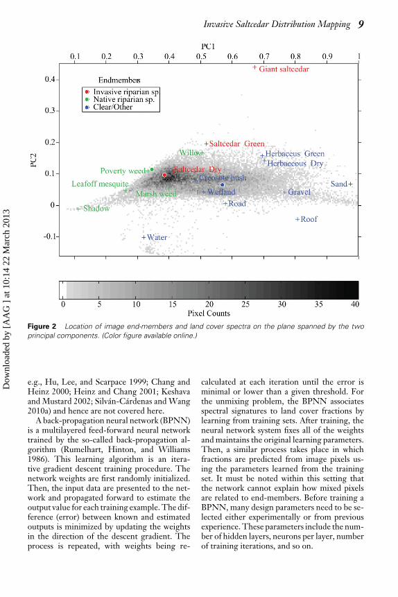
End-Member SelectionIn this study, three end-members were defined:invasive species, native species, and clear. Spec-

tral reflectances for each end-member were de-rived from the training data collected in thefield and from the AISA image. The end-members are plotted in Figure 2, which showsthe location of each end-member on the planespanned by the two principal components,which explain 99.6 percent of the total variance.It also shows the two-dimensional histogramof mixed pixels (background image) and pointsfrom a set of signatures for sixteen land-coverclasses laid out in Table 1 (labeled crosses).These signatures were selected from theoriginal AISA imagery with the aid of GPSpoints acquired in the field. The signatureswere resampled to match the TM spectral char-acteristic and then projected onto the PCAplane. Each land-cover type in Table 1 was as-signed to one of the three categories used (asindicated by the color): invasive (red), native(green), and clear (blue). The two-dimensionalplot reflects the major data distribution, thusrevealing that the end-member for the invasivecategory is interior to the cloud of mixed pixels.

Species Abundance Mapping with Linearand Nonlinear Spectral UnmixingFour LSU and three NN mixture modelswere adopted to derive subpixel abundances ofsaltcedar. The general LSU mixture model isexpressed in Equation 1:

y = Xα+ ∈ (1)

where the matrix X is formed by three end-members, y stands for the observed mixed pix-els, α is the abundance or land-cover fractionsto be estimated, and ε represents residual errorthat is not explained by the three end-members.

Given that end-members and mixed pix-els are known, Equation 1 can be solved us-ing the least squares (LS) approach, with orwithout constraints. Here we applied four LSformulations: (1) without constraint (uncon-strained LSU, or UCLSU), (2) with unit sumof fractions constraint (sum-constrained LSUor SCLSU), (3) with nonnegative fractionconstraint (nonnegativity constrained LSU orNCLSU), and (4) with both unit sum and non-negative fraction constraints (fully constrainedLSU or FCLSU). Details on the formula-tion and algorithms for each method havebeen provided in a number of references (see,

Dow

nloa

ded

by [

AA

G ]

at 1

0:14

22

Mar

ch 2

013

Invasive Saltcedar Distribution Mapping 9

Figure 2 Location of image end-members and land cover spectra on the plane spanned by the twoprincipal components. (Color figure available online.)

e.g., Hu, Lee, and Scarpace 1999; Chang andHeinz 2000; Heinz and Chang 2001; Keshavaand Mustard 2002; Silvan-Cardenas and Wang2010a) and hence are not covered here.

A back-propagation neural network (BPNN)is a multilayered feed-forward neural networktrained by the so-called back-propagation al-gorithm (Rumelhart, Hinton, and Williams1986). This learning algorithm is an itera-tive gradient descent training procedure. Thenetwork weights are first randomly initialized.Then, the input data are presented to the net-work and propagated forward to estimate theoutput value for each training example. The dif-ference (error) between known and estimatedoutputs is minimized by updating the weightsin the direction of the descent gradient. Theprocess is repeated, with weights being re-

calculated at each iteration until the error isminimal or lower than a given threshold. Forthe unmixing problem, the BPNN associatesspectral signatures to land cover fractions bylearning from training sets. After training, theneural network system fixes all of the weightsand maintains the original learning parameters.Then, a similar process takes place in whichfractions are predicted from image pixels us-ing the parameters learned from the trainingset. It must be noted within this setting thatthe network cannot explain how mixed pixelsare related to end-members. Before training aBPNN, many design parameters need to be se-lected either experimentally or from previousexperience. These parameters include the num-ber of hidden layers, neurons per layer, numberof training iterations, and so on.

Dow

nloa

ded

by [

AA

G ]

at 1

0:14

22

Mar

ch 2

013

10 Volume 65, Number 1, February 2013

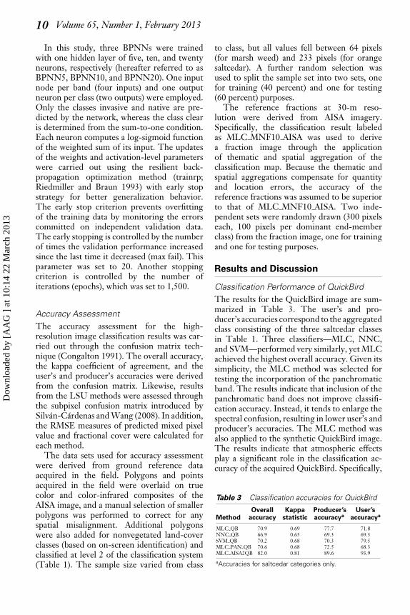
In this study, three BPNNs were trainedwith one hidden layer of five, ten, and twentyneurons, respectively (hereafter referred to asBPNN5, BPNN10, and BPNN20). One inputnode per band (four inputs) and one outputneuron per class (two outputs) were employed.Only the classes invasive and native are pre-dicted by the network, whereas the class clearis determined from the sum-to-one condition.Each neuron computes a log-sigmoid functionof the weighted sum of its input. The updatesof the weights and activation-level parameterswere carried out using the resilient back-propagation optimization method (trainrp;Riedmiller and Braun 1993) with early stopstrategy for better generalization behavior.The early stop criterion prevents overfittingof the training data by monitoring the errorscommitted on independent validation data.The early stopping is controlled by the numberof times the validation performance increasedsince the last time it decreased (max fail). Thisparameter was set to 20. Another stoppingcriterion is controlled by the number ofiterations (epochs), which was set to 1,500.

Accuracy AssessmentThe accuracy assessment for the high-resolution image classification results was car-ried out through the confusion matrix tech-nique (Congalton 1991). The overall accuracy,the kappa coefficient of agreement, and theuser’s and producer’s accuracies were derivedfrom the confusion matrix. Likewise, resultsfrom the LSU methods were assessed throughthe subpixel confusion matrix introduced bySilvan-Cardenas and Wang (2008). In addition,the RMSE measures of predicted mixed pixelvalue and fractional cover were calculated foreach method.

The data sets used for accuracy assessmentwere derived from ground reference dataacquired in the field. Polygons and pointsacquired in the field were overlaid on truecolor and color-infrared composites of theAISA image, and a manual selection of smallerpolygons was performed to correct for anyspatial misalignment. Additional polygonswere also added for nonvegetated land-coverclasses (based on on-screen identification) andclassified at level 2 of the classification system(Table 1). The sample size varied from class

to class, but all values fell between 64 pixels(for marsh weed) and 233 pixels (for orangesaltcedar). A further random selection wasused to split the sample set into two sets, onefor training (40 percent) and one for testing(60 percent) purposes.

The reference fractions at 30-m reso-lution were derived from AISA imagery.Specifically, the classification result labeledas MLC MNF10 AISA was used to derivea fraction image through the applicationof thematic and spatial aggregation of theclassification map. Because the thematic andspatial aggregations compensate for quantityand location errors, the accuracy of thereference fractions was assumed to be superiorto that of MLC MNF10 AISA. Two inde-pendent sets were randomly drawn (300 pixelseach, 100 pixels per dominant end-memberclass) from the fraction image, one for trainingand one for testing purposes.

Results and Discussion

Classification Performance of QuickBirdThe results for the QuickBird image are sum-marized in Table 3. The user’s and pro-ducer’s accuracies correspond to the aggregatedclass consisting of the three saltcedar classesin Table 1. Three classifiers—MLC, NNC,and SVM—performed very similarly, yet MLCachieved the highest overall accuracy. Given itssimplicity, the MLC method was selected fortesting the incorporation of the panchromaticband. The results indicate that inclusion of thepanchromatic band does not improve classifi-cation accuracy. Instead, it tends to enlarge thespectral confusion, resulting in lower user’s andproducer’s accuracies. The MLC method wasalso applied to the synthetic QuickBird image.The results indicate that atmospheric effectsplay a significant role in the classification ac-curacy of the acquired QuickBird. Specifically,

Table 3 Classification accuracies for QuickBird

MethodOverall

accuracyKappa

statisticProducer’saccuracya

User’saccuracya

MLC QB 70.9 0.69 77.7 71.8NNC QB 66.9 0.65 69.3 69.3SVM QB 70.2 0.68 70.3 79.5MLC PAN QB 70.6 0.68 72.5 68.3MLC AISA2QB 82.0 0.81 89.6 93.9

aAccuracies for saltcedar categories only.

Dow

nloa

ded

by [

AA

G ]

at 1

0:14

22

Mar

ch 2

013

Invasive Saltcedar Distribution Mapping 11

Table 4 Classification accuracies for Airborne Imaging Spectroradiometer for Applications imagery

Method Overall accuracy Kappa statistic Producer’s accuracya User’s accuracya

SAM AISA61 68.6 0.66 84.8 94.7MMF AISA61 45.0 0.42 45.8 78.6MLC AISA4 84.5 0.83 89.4 91.4NNC AISA4 63.9 0.62 95.1 87.1SVM AISA4 86.6 0.86 92.7 94.9MLC LDA7 AISA 86.6 0.86 92.7 94.9SVM LDA7 AISA 85.8 0.85 91.9 94.8MLC MNF10 AISA 87.6 0.87 93.7 94.6SVM MNF10 AISA 87.7 0.87 93.9 96.5

aAccuracies for saltcedar categories only.

the overall accuracy from the synthetic imageincreased more than 10 percent with respect tothe acquired QuickBird.

Classification Performance of AISAThe results for the AISA image are summa-rized in Table 4. Because the AISA image con-tains more detailed spectral information, higheroverall and individual classification accuracieswere expected. Results indicate, however, thatthe processing of hyperspectral data must bedone with much care. The methods that utilizeall of the hyperspectral bands (SAM and MMF)

performed poorer when compared to the re-sults from QuickBird. Band selection generallyincreased the performance even for the casewhere only the four narrow bands that alignedwith the QuickBird bandpass filters were se-lected. The best band selection method wasthe MNF. The SVM gave the highest accuracywhen the MNF band selection was adopted.Yet, the MLC performed very close to SVM. Areason for this might be due to the fact that allof the classes defined in this study do not exhibitcomplex spectral variability. In fact, the spec-tral variability of saltcedar was largely avoidedby differentiating three subclasses: saltcedar

Table 5 Coefficients for the optimal linear transformation from linear discriminant analysis (LDA)

AISA band LDA1 LDA2 LDA3 LDA4 LDA4 LDA6 LDA7 LDA8

8 454.27 0.30399 463.31 0.369411 481.39 0.296712 490.42 0.336614 508.50 −0.3406 0.314815 517.54 −0.3251 −0.469516 526.58 −0.519317 535.61 −0.336418 544.67 0.408119 553.89 −0.3318 0.2827 −0.448921 572.45 0.5569 0.4744 0.436522 581.78 0.3525 −0.4277 0.498923 591.18 −0.562324 600.58 −0.5106 −0.7204 −0.360425 609.98 −0.44726 619.39 0.3176 −0.543527 628.79 −0.283729 647.59 0.5915 −0.741331 666.39 0.425232 675.80 0.51533 685.20 0.316335 704.02 −0.449436 713.45 0.5059

Note: Blanks represent zeros. AISA = Airborne Imaging Spectroradiometer for Applications.

Dow

nloa

ded

by [

AA

G ]

at 1

0:14

22

Mar

ch 2

013

12 Volume 65, Number 1, February 2013

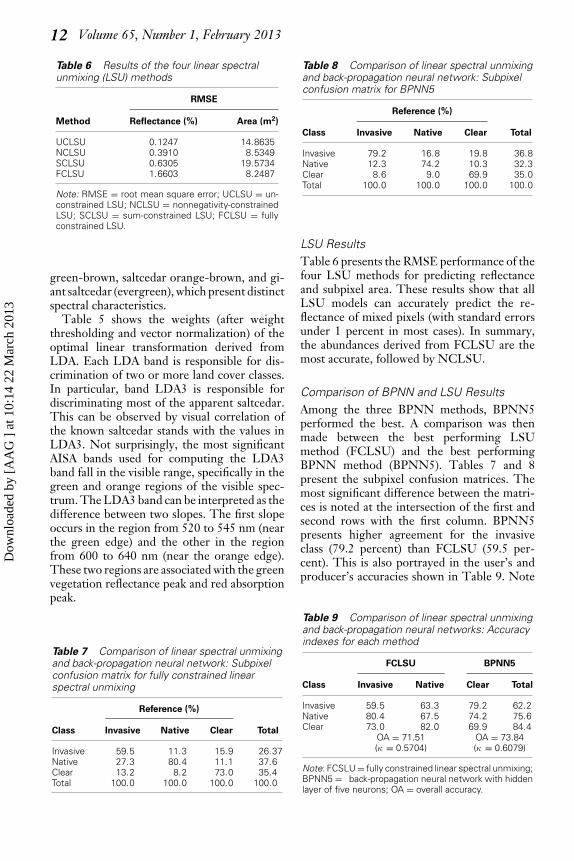
Table 6 Results of the four linear spectralunmixing (LSU) methods

RMSE

Method Reflectance (%) Area (m2)

UCLSU 0.1247 14.8635NCLSU 0.3910 8.5349SCLSU 0.6305 19.5734FCLSU 1.6603 8.2487

Note: RMSE = root mean square error; UCLSU = un-constrained LSU; NCLSU = nonnegativity-constrainedLSU; SCLSU = sum-constrained LSU; FCLSU = fullyconstrained LSU.

green-brown, saltcedar orange-brown, and gi-ant saltcedar (evergreen), which present distinctspectral characteristics.

Table 5 shows the weights (after weightthresholding and vector normalization) of theoptimal linear transformation derived fromLDA. Each LDA band is responsible for dis-crimination of two or more land cover classes.In particular, band LDA3 is responsible fordiscriminating most of the apparent saltcedar.This can be observed by visual correlation ofthe known saltcedar stands with the values inLDA3. Not surprisingly, the most significantAISA bands used for computing the LDA3band fall in the visible range, specifically in thegreen and orange regions of the visible spec-trum. The LDA3 band can be interpreted as thedifference between two slopes. The first slopeoccurs in the region from 520 to 545 nm (nearthe green edge) and the other in the regionfrom 600 to 640 nm (near the orange edge).These two regions are associated with the greenvegetation reflectance peak and red absorptionpeak.

Table 7 Comparison of linear spectral unmixingand back-propagation neural network: Subpixelconfusion matrix for fully constrained linearspectral unmixing

Reference (%)

Class Invasive Native Clear Total

Invasive 59.5 11.3 15.9 26.37Native 27.3 80.4 11.1 37.6Clear 13.2 8.2 73.0 35.4Total 100.0 100.0 100.0 100.0

Table 8 Comparison of linear spectral unmixingand back-propagation neural network: Subpixelconfusion matrix for BPNN5

Reference (%)

Class Invasive Native Clear Total

Invasive 79.2 16.8 19.8 36.8Native 12.3 74.2 10.3 32.3Clear 8.6 9.0 69.9 35.0Total 100.0 100.0 100.0 100.0

LSU ResultsTable 6 presents the RMSE performance of thefour LSU methods for predicting reflectanceand subpixel area. These results show that allLSU models can accurately predict the re-flectance of mixed pixels (with standard errorsunder 1 percent in most cases). In summary,the abundances derived from FCLSU are themost accurate, followed by NCLSU.

Comparison of BPNN and LSU ResultsAmong the three BPNN methods, BPNN5performed the best. A comparison was thenmade between the best performing LSUmethod (FCLSU) and the best performingBPNN method (BPNN5). Tables 7 and 8present the subpixel confusion matrices. Themost significant difference between the matri-ces is noted at the intersection of the first andsecond rows with the first column. BPNN5presents higher agreement for the invasiveclass (79.2 percent) than FCLSU (59.5 per-cent). This is also portrayed in the user’s andproducer’s accuracies shown in Table 9. Note

Table 9 Comparison of linear spectral unmixingand back-propagation neural networks: Accuracyindexes for each method

FCLSU BPNN5

Class Invasive Native Clear Total

Invasive 59.5 63.3 79.2 62.2Native 80.4 67.5 74.2 75.6Clear 73.0 82.0 69.9 84.4

OA = 71.51(κ = 0.5704)

OA = 73.84(κ = 0.6079)

Note: FCSLU = fully constrained linear spectral unmixing;BPNN5 = back-propagation neural network with hiddenlayer of five neurons; OA = overall accuracy.

Dow

nloa

ded

by [

AA

G ]

at 1

0:14

22

Mar

ch 2

013

Invasive Saltcedar Distribution Mapping 13

Table 10 Comparison of linear spectralunmixing and back-propagation neural network:Computation cost

Time (msec)

Method Parameters Train (300) Test (600)

FCLSU 12 0 1,756BPNN5 37 7,718 30

Note: FCSLU = FCSLU = fully constrained linear spec-tral unmixing; BPNN5 = back-propagation neural networkwith hidden layer of five neurons.

the higher difference in producer’s accuraciesfrom FCLSU with respect to producer’saccuracies from BPNN5. A marginal improve-ment of around 2 percent was obtained fromBPNN5, as given by the overall accuracy (OA).The number of parameters and computer timerequired by each classifier are presented in Ta-ble 10. The central processing unit (CPU) timerequired for the training and testing were mea-sured in MATLAB. The processing used a SonyVaio laptop with Pentium 4 CPU running at 2.8GHz with 512 MB of RAM. The training timefor FCLSU consists of the computation timeof the end-members, which was negligible be-cause training data were available, whereas thetraining time for the BPNN5 was around 8 sec-onds. In contrast, FCLSU required much moretime than BPNN5 by nearly a factor of sixty.

Conclusions

To examine the potential of contemporary re-mote sensing for mapping saltcedar at dif-ferent spatial scales, a comprehensive studywas conducted using multiresolution, multi-source remote sensing imagery encompassingQuickBird, AISA, and Landsat TM. Resultsindicate that AISA hyperspectral imagery out-performed QuickBird imagery in differentiat-ing saltcedar from other riparian vegetationspecies. SVM achieved the highest classifica-tion accuracy among the five adopted classi-fiers. LSU methods exhibited similar mappingaccuracy to NN methods in estimating abun-dance of saltcedar at a spatial resolution of30 × 30 m2 but with significantly better com-puting efficiency, which is an important factorthat should be taken into account for tacklingregional-scale saltcedar spread from remote

sensing. Overall, this study investigates manyof the best capabilities of contemporary remotesensing for assisting with the reconnaissance ofsaltcedar, one of the most threatening invasivespecies in the southwestern United States. �

Literature Cited

Adams, J. B., M. O. Smith, and A. R. Gillespie.1993. Imaging spectroscopy: Interpretation basedon spectral mixture analysis. In Remote geochemi-cal analysis: Elemental and mineralogical composition,ed. C. M. Pieters and P. Englert, 145–66. Boston:Cambridge University Press.

Baum, B. R. 1967. Introduced and naturalizedtamarisks in the United States and Canada [Tamar-icaceae]. Baileya 15:19–25.

Benediktsson, J. A., P. H. Swain, and O. K. Er-soy. 1990. Neural network approaches versusstatistical-methods in classification of multisourceremote-sensing data. IEEE Transactions on Geo-science and Remote Sensing 4:540–52.

Boardman, J. W., F. A. Kruse, and R. O. Green.1995. Mapping target signatures via partial unmix-ing of AVIRIS data. In Summaries, Fifth JPL Air-borne Earth Science Workshop. JPL Publication 95-1,1:23–26. Washington, DC: Jet Propulsion Labo-ratory.

Chang, C.-I., and D. C. Heinz. 2000. Constrainedsub-pixel target detection of remotely sensed im-agery. IEEE Transactions on Geoscience and RemoteSensing 38 (3): 1114–59.

Cleverly, J. R., S. D. Smith, A. Sala, and D. A. Devitt.1997. Invasive capacity of Tamarix ramosissima ina Mojave Desert floodplain: The role of drought.Oecologia 111:12–18.

Congalton, R. G. (1991). A review of assess-ing the accuracy of classifications of remotelysensed data. Remote Sensing of Environment 37:35–46.

ENVI version 4.1, ITT Visual Information Solu-tions (formerly Research Systems, Inc.), Boulder,CO.

Everitt, J. H., C. Yang, and M. R. Davis. 2004. Re-mote mapping of two invasive weeds in the RioGrande system of Texas. Paper presented at theAmerican Water Resources Association Confer-ence, Orlando, FL.

Frazier, A. E., and L. Wang. 2011. Characteriz-ing spatial patterns of invasive species using sub-pixel classifications. Remote Sensing of Environment115:1997–2007.

Fuller, D. O. 2005. Remote detection of inva-sive Malameuca trees (Malaleuca quinquenervia) inSouth Florida with multispectral IKONOS im-agery. International Journal of Remote Sensing 26 (5):1057–63.

Dow

nloa

ded

by [

AA

G ]

at 1

0:14

22

Mar

ch 2

013

14 Volume 65, Number 1, February 2013

Glenn, N. F., J. T. Mundt, K. T. Weber, T. S.Prather, L. W. Lass, and J. Pettingill. 2005. Hy-perspectral data processing for repeat detection ofsmall infestations of leafy spurge. Remote Sensing ofEnvironment 95:399–412.

Hamada, Y., D. A. Stow, L. L. Coulter, J. C.Jafolla, and L. W. Hendricks. 2007. DetectingTamarisk species (Tamarix spp.) in riparian habi-tats of Southern California using high spatial res-olution hyperspectral imagery. Remote Sensing ofEnvironment 109 (2): 237–48.

Heinz, D. C., and C.-I. Chang. 2001. Fully con-strained least square linear spectral unmixing anal-ysis method for material quantification in hyper-spectral imagery. IEEE Transactions on Geoscienceand Remote Sensing 39 (3): 529–45.

Hu, Y. H., H. B. Lee, and F. L. Scarpace. 1999.Optimal linear spectral unmixing. IEEE Transac-tions on Geoscience and Remote Sensing 37 (1): 639–44.

Kavzoglu, T., and P. M. Mather. 2003. The use ofbackpropagation artificial neural networks in landcover classification. International Journal of RemoteSensing 24 (23): 4907–38.

Keshava, N., and J. F. Mustard. 2002. Spectral unmix-ing. IEEE Signal Processing Magazine 19 (1): 44–57.

Kruse, F. A., J. W. Boardman, and J. F. Huntington.2003. Comparison of airborne hyperspectral dataand EO-1 Hyperion for mineral mapping. IEEETransactions on Geoscience and Remote Sensing 41 (6):1388–1400.

Kruse, F. A., A. B. Lefkoff, J. W. Boardman, K. B.Heidebrecht, A. T. Shapiro, P. J. Barloon, and A.F. H. Goetz. 1993. The Spectral Image ProcessingSystem (SIPS)—Interactive visualization and anal-ysis of imaging spectrometer data. Remote Sensingof Environment 44:145–63.

Lass, L. W., and T. S. Prather. 2004. Detecting thelocations of Brazilian pepper trees in the Ever-glades with hyperspectral sensor. Weed Technology18437–42.

Lass, L. W., T. S. Prather, N. F. Glenn, K. T. We-ber, J. T. Mundt, and J. Pettingill. 2005. A reviewof remote sensing of invasive weeds and exam-ple of early detection of spotted knapweed (Cen-taurea maculosa) and babysbreath (Gypsophila pan-iculata) with a hyperspectral sensor. Weed Science53:242–51.

MATLAB version 6.5.1. Natick, MA: The Math-works Inc.

Morisette, J. T., C. S. Jarnevich, A. Ullah, W. Cai,J. A. Pedelty, J. E. Gentle, T. J. Stohlgren, andJ. L. Schnase. 2006. A Tamarisk habitat suitabilitymap for the continental United States. Frontiers inEcology and the Environment 4 (1): 11–17.

O’Neill, M., S. L. Ustin, S. Hager, and R. Root.2000. Mapping the distribution of leafy spurge atTheodore Roosevelt National Park using AVIRIS.

Paper presented at the Ninth JPL Airborne VisibleInfrared Imaging Spectrometer (AVIRIS) Work-shop, Jet Propulsion Laboratory, Pasadena, CA.

Pu, R., P. Gong, Y. Tian, X. Miao, and R. Car-ruthers. 2008. Using classification and NDVI dif-ferencing methods for monitoring sparse vegeta-tion coverage: A case study of saltcedar in Nevada,USA. International Journal of Remote Sensing 29(14): 1987–2011.

Richards, J. A., and X. Jia. 1999. Remote sensing digitalimage analysis. 3rd ed. Berlin: Springer-Verlag.

Riedmiller, M., and H. Braun. 1993. A direct adaptivemethod for faster back propogation learning: TheRPROP algorithm. In Proceedings of the IEEE In-ternational Conference on Neural Networks, 586–90.San Francisco, CA.

Rumelhart, D. E., G. E. Hinton, and R.J. Williams. 1986. Learning representationsby back-propagating errors. Nature 323:533–36.

Silvan-Cardenas, J., and L. Wang. 2008. Sub-pixelconfusion-uncertainty matrix for assessing softclassifications. Remote Sensing of Environment 112(3): 1081–95.

———. 2010a. Fully constrained linear spectral un-mixing: Analytic solution using fuzzy sets. IEEETransactions on Geoscience and Remote Sensing 48(11): 3992–4002.

———. 2010b. Retrieval of subpixel Tamarix canopycover from Landsat data along the ForgottenRiver using linear and nonlinear spectral mixturemodels. Remote Sensing of Environment 114:1777–90.

Underwood, E., S. Ustin, and D. DiPietro. 2003.Mapping non native plants using hyperspectralimagery. Remote Sensing of Environment 86:150–61.

William, P. A., and E. R. Hunt. 2002. Estimation ofleafy spurge cover from hyperspectral imagery us-ing mixture tuned matched filtering. Remote Sensingof Environment 82:446–56.

Wu, T.-F., C.-J. Lin, and R. C. Weng. 2004. Prob-ability estimates for multi-class classification bypairwise coupling. Journal of Machine Learning Re-search 5:975–1005.

LE WANG is a visiting scholar in the State KeyLaboratory of Earth Surface Processes and ResourceEcology, Beijing Normal University, 19 XinjiekouWai St., Hai Dian District, Beijing 100875, P. R.China. E-mail: lewang@buffalo.edu. He also serves asassociate professor of Geography at the State Univer-sity of New York, Buffalo, NY. His research centerson development of advanced remote sensing tech-niques for estimating small-area urban populations,mapping and monitoring coastal mangrove forests,and mapping and modeling the spread of invasive

Dow

nloa

ded

by [

AA

G ]

at 1

0:14

22

Mar

ch 2

013

Invasive Saltcedar Distribution Mapping 15

species. He was the recipient of the 2008 Early Ca-reer Awards from Remote Sensing specialty group ofthe Association of American Geographers (AAG).

JOSE L. SILVAN-CARDENAS is associate profes-sor of the Centro de Investigacion en Geografıa yGeomatica “Ing. Jorge L. Tamayo,” A.C. Contoy137, Lomas de Padierna, Mex. D.F. 14240, Mex-ico. E-mail: jlsilvan@centrogeo.org.mx. His researchinterest includes feature extraction from light detec-tion and ranging (LiDAR) data and spectral mixturemodeling for hyperspectral image analysis. He wasthe recipient of the 2010 Warren L. Nystrom Awardfrom the AAG.

JUN YANG is professor of forestry at the Col-lege of Forestry, Beijing Forestry University, Beijing100083, China. E-mail: larix001@gmail.com. His re-search interests include the impact of global climatechange on urban ecosystems and modeling of modi-fication of microclimate by urban vegetation.

AMY E. FRAZIER is a doctoral candidate in the De-partment of Geography at the State University ofNew York, 105 Wilkeson Quad, Buffalo, NY 14261.E-mail: amy.frazier@gmail.com. Her research inter-ests focus on modeling structural patterns of invasivespecies and integrating subpixel remote sensing clas-sifications with landscape metric analyses.

Dow

nloa

ded

by [

AA

G ]

at 1

0:14

22

Mar

ch 2

013