Introductory Tutorial for “Discover” - NCCS’s newest Linux ...

Introductory Tutorial for “Discover” -NCCS’s newest Linux Networx Cluster

by

Software Integration and Visualization Office (SIVO)

Introduction to SIVOWho we are:• Leadership in

– the development of advanced scientific software– industry best practices that minimize risk and cost

• Competency in– state-of-the-art visualization tools and techniques– computational science– modern software engineering practices

• Have an established and cordial relationship with NASAscientific research community

What services we provide:• HPC services, Parallelization, Tuning & Debugging• Scientific code re-factoring and redesign• Object Oriented Design (OOD) of science applications• State-of-the-art visualization support

Contact information:http://sivo.gsfc.nasa.gov/

Training Outline

• Overview of System Architecture

• Accessing the System

• File Systems

• Programming Environment

• Compiling/Optimization

• How to Run/ Debugging

• Tools for Performance and Data Analysis

UdayaRanawake

BruceVan Aartsen

HamidOloso

Overview of System Architecture - Nodes

• 4 Front-end nodes• 128 Compute Nodes:

– SuperMicro mother board, 0.8UEvolocity II chassis

– Dual Socket , dual core(4 cores per node)

– 120 GB hard drive– 4 GB RAM

Overview of System Architecture - Processor

• Base Unit:– Intel Dempsey Dual Core 3.2GHz (Xeon 5060)– 1066 MHz front side bus– 2 MB L2 cache per core (4 MB total per socket)– 12.8 GFLOPS/socket peak performance (25.6

GF/node)• Early indications with High Performance Linpack

(HPL) are showing 60% - 65% of peak

Overview of System Architecture - Memory

• 4 GB RAM/node (4 x 1 GB DDR2 533 MHz)– Only 3GB user-accessible

• Memory bandwidth 4 GB/s to the core• Each core has its own Levels 1 and 2 cache

– Level 1 cache (Unified Instruction/Data, 32KB)– Level 2 cache (Separate Instruction and data, 2 MB

each)

Overview of System Architecture - Interconnect

• Dual-ported 4x InfiniBand Host Channel Adapters(HCA)‒ PCI-Express 8x (10 Gb/s)– Aggregate Bandwidth - 20 Gb/s bi-directional– Latency: ~4 microseconds

Overview of System Architecture -Comparison

3.2~73.3Peak Performance(TFLOPS)

HP Alpha SC45

‘Halem’

SGI Altix‘Palm/

Explore’Linux Networx

‘Discover’Platform

Tru64 UNIXSGI AdvancedLinux Environ.(RHEL based)

SUSE LinuxOperating System

696272/2048512Total memory (GB)

34864/512128Total number of nodes

Overview of System Architecture - Future plan

• Scalable Expansion Nodes– Dell mother board 1U chassis‒ Dual socket, dual core Intel Woodcrest 2.66 GHz

• Both cores share 4MB L2 cache– 4 GB DDR2 667 MHz FB DIMM– 160 GB hard drive

• Visualization Nodes– 16 nodes integrated into the base unit– AMD Opteron dual core 280 processors (2.6 GHz)– 8 GB of PC3200/DDR400 S/R DIMM– 250 GB SATA– NVidia Quadro FX 4500 PCI-Express

Accessing the System - Requirements

• Need an active account– [email protected]

• Need RSA securID fob– http://nccs.gsfc.nasa.gov/

Accessing the System - Local (GSFC/NASA)

• From GSFC hosts, log onto discover using:ssh [-XY] [email protected]

• X or Y are optional, enable X11 forwarding.• Passcode:10 digit ID number: 4-digit PIN + 6-digit fob• Host: discover• Password: requires user password.• Note: discover is in LDAP (Lightweight Directory Access

Protocol), enables password sharing with other system inLDAP

Accessing the System - Remote (offsite)

• Login from other NASA hosts:Login into GSFC hosts to access login.nccs.nasa.gov

• Login from non-NASA hosts:– Provide host name(s) or IP address to

[email protected]– Entry through login.gsfc.nasa.gov.– Alternatively, apply for GSFC VPN account

File Systems - /discover/home/discover/nobackup

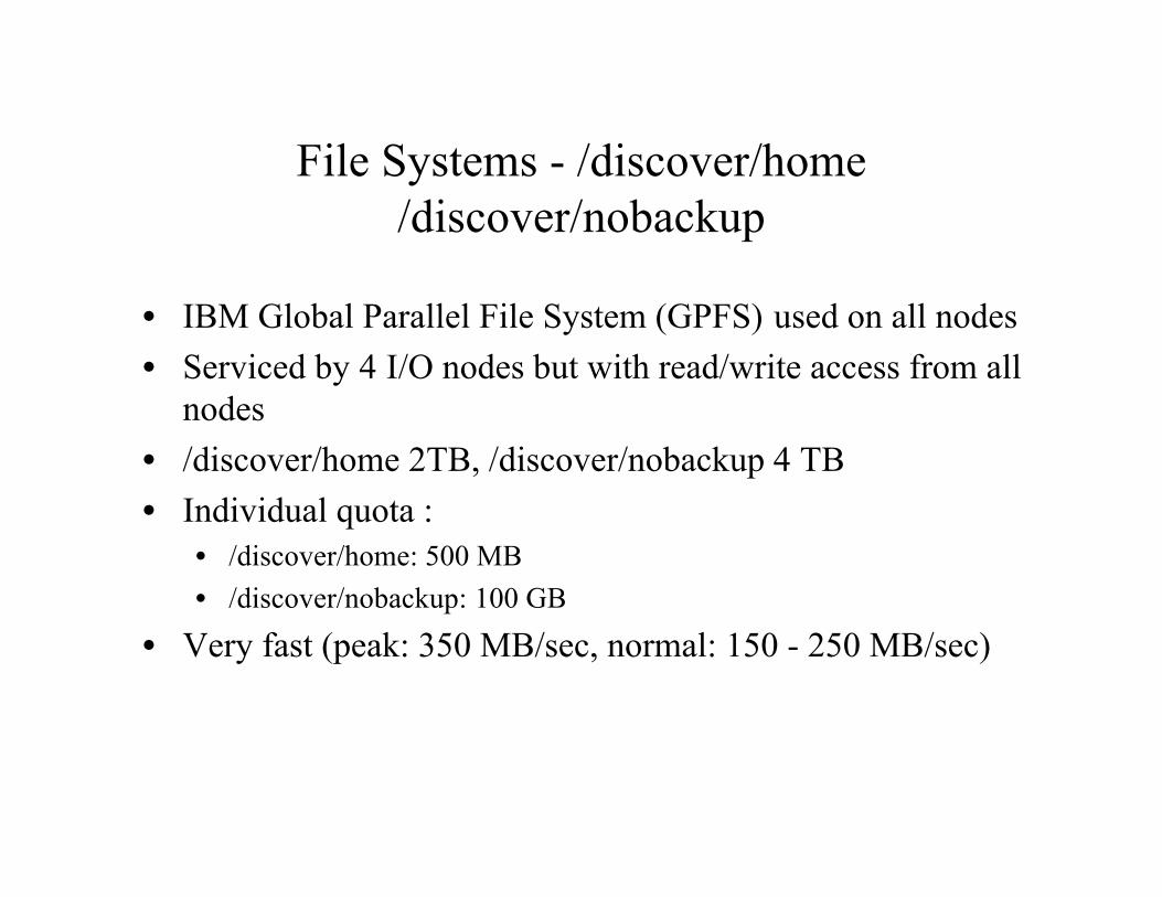
• IBM Global Parallel File System (GPFS) used on all nodes• Serviced by 4 I/O nodes but with read/write access from all

nodes• /discover/home 2TB, /discover/nobackup 4 TB• Individual quota :

• /discover/home: 500 MB• /discover/nobackup: 100 GB

• Very fast (peak: 350 MB/sec, normal: 150 - 250 MB/sec)

File Systems - Overview

Disk

128 Compute Nodes

4 Login Nodes

2 Gateway Nodes

4 I/O Nodes

IB

DDN Control.

10 GigE

1 GigESAN

File Systems - /discover/nobackup - Cont’d

• Recommended for running jobs (more space)• Not backed up• Stage data in before a run• Stage data out after a run• For large data transfer , higher transfer rates

(shared 10GB/sec) possible via data transfercommands in a script submitted to datamovequeue

File Systems - Mass Storage (dirac)

• Mass storage: dirac.gsfc.nasa.gov• Access using ssh, scp, sftp, ftp (anonymous)

File Systems - Moving Data In or Out

• Moving/copying files into and out of the system– scp : file transfer to and from dirac.gsfc.nasa.gov– sftp, ftp : file transfer from dirac.gsfc.nasa.gov– dmf: ssh into required system and execute dmf related

commands locally

Programming Environment

• Programming environment is controlled usingmodules

• No modules are loaded by default. The user has toadd the needed modules to the shell startup file.

• Checking available modules• module avail

• Checking loaded modules• module list

• Unloading a module• module unload <module name>

• Loading a module• module load <module name>

• Swapping modules• module swap <old module> <new module>

• Purging all modules• module purge

Programming Environment cont’d

• Typical module commands for shell startup file• Initialization for tcsh

– source /usr/share/modules/init/tcsh

• Initialization for csh– source /usr/share/modules/init/csh

• Initialization for bash– ./usr/share/modules/init/bash

• module purge

• module load comp/intel-9.1.039

• module load mpi/scali-5.1.0.1• module load lib/mkl-9.0.017


• Things to remember:

• No modules are loaded at login. Explicitly loadthe required modules.

• Your MKL module must match the compilerversion.


Compiling

• How to compile:

• Different versions of Intel compilers are available• To see available compilers: module avail

• To see loaded compiler: module list

• Use an appropriate “module” command to selectanother compiler

Compiling - Sequential Build

Intel compilers• ifort <flags> code.f (or .f90)

• icc <flags> code.c

• icpc <flags> code.cpp (or .C)

Compiling - OpenMP Build

Intel compilers• ifort -openmp <flags> code.f (or .f90)

• icc -openmp <flags> code.c

• icpc -openmp <flags> code.cpp (or .C)

Compiling - MPI Build

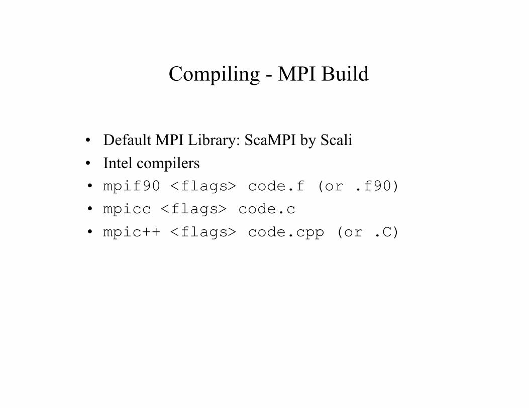
• Default MPI Library: ScaMPI by Scali• Intel compilers• mpif90 <flags> code.f (or .f90)

• mpicc <flags> code.c

• mpic++ <flags> code.cpp (or .C)

Optimization and Debugging Flags

• -O0: No optimization.• -O2: Default optimization level.• -O3: Includes more software pipelining, prefetching, and loop

reorganization.• -g : Generates symbolic debugging information and line

numbers in the object code for use by source-level debuggers.• -openmp: Enables the parallelizer to generate multithreaded

code based on the OpenMP directives.

Optimization and Debugging Flags contd.

• -traceback: Available in Version 8 and highercompilers only.– Tells the compiler to generate extra information in the object file

to allow the display of source file traceback information at runtimewhen a severe error occurs. The default is -notraceback.

Some things to Remember

• If the build fails:– Check the compiler version; you may need to swap modules– Check the optimization level; a different level might work

• If the link fails:– Check that environment variables include the correct paths

• If you see the following errors during link:/usr/local/intel/fce/8.1.032/lib/libcxa.so.5: undefined reference to

uw_parse_lsda_info….Try adding -lunwind to your link flags

• If you see the following warning during link:/usr/local/intel/fce/9.1.036/lib/libimf.so: warning; warning: feupdateenv

is not implemented and will always fail….Try adding -i_dynamic option to your link flags

Third Party Libraries

• Will be installed under /usr/local/other.• Baselibs will be in this directory.• Some of the important software packages available under

baselibs are:– esmf– netcdf– hdf

How to Run• Uses PBS Queuing System• Queues described below, with * notations defined on next slide

Resource limitQueue name

≤ 4≤ 64background

≤ 3≤ 8pproc≤ 11datamove (**)

(***)(***)router

≤ 1≤ 8debug≥ 3, ≤ 12≤ 4general_small≤ 12≤ 32general≤ 24≤ 128general_hi (*)≤ 12≤ 128high_priority (*)Wall (hours)# nodes

(*) Restricted; requires permission

(**) Queue specifically set up for fast data transfer. Mapped to gateway nodes. Allows up to four data movement jobs per gateway node

(***) “router” is the default when no queue has been selected. Appropriately maps jobs to one of debug, pproc, general_small and general.

How to Run cont’d

• Frequently used commands– qsub: To submit a job

•qsub myscript

– qstat: To check job status•qstat -a for all jobs•qstat -au myuserid for my jobs alone•qstat -Q[f] to see what queues are available.

Adding the “f” option provides details.

– qdel: To delete a job from the queue•qdel jobid (Obtain jobid from qstat)

How to Run cont’d

• Interactive batch:qsub -V -I -l select=4,walltime=04:00:00

– -V exports user’s environment to the PBS job– -I implies an interactive batch session– -l requests resources e.g. 4 nodes and 4 hrs of wall time– You will get a terminal session that you can use for

regular interactive activities

• Batch:– qsub <batch_script>

How to Run cont’d

• #PBS -W group_list=<value> - To specify group name(s) underwhich this job should run

• #PBS -m mail_options - To control condition under which mailabout the job is sent. Mail_options can be any combination of “a” (sendmail when job aborts), “b” (send mail when job begins execution) and“c” ( send mail when job terminates)

• #PBS -l resource=<value> - To request resource e.g.:– #PBS -l select=4 - To requests four execution units or nodes– #PBS -l walltime=4:00:00 - To request 4 hours of run time

How to Run cont’d: Common PBS options

How to Run cont’d: Common PBS options

• #PBS -o myjob.out - To redirect standard output to myjob.out• #PBS -e myjob.err - To redirect standard error to myjob.err• #PBS -j oe - To merge std output and std error into standard output• #PBS -j eo - To merge std output and std error into standard error• #PBS -N myjob - To set the job name to myjob, else job name is

script name• Useful PBS environmental variable is $PBS_O_WORKDIR. It is the

absolute path to the directory where a PBS job is submitted from

#!/bin/csh -f#PBS -W group_list=g0000

#PBS -m e#PBS -l select=4

#PBS -l walltime=4:00:00#PBS -o myjob.out

#PBS -j oe#PBS -N myjob

cd $PBS_O_WORKDIR

# For MPI job.# Note: Run maximum of 4 processes per node.

# Depending on application, fewer processes per node# may be better

mpirun -np 16 -inherit_limits ./myjob

How to Run cont’d: Example MPI batch script

#!/bin/csh -f

#PBS -W group_list=g0000

#PBS -m e

#PBS -l select=1

#PBS -l walltime=4:00:00

#PBS -o myjob.out

#PBS -j oe

#PBS -N myjob

cd $PBS_O_WORKDIR

# For serial job

./myjob

How to Run cont’d: Example serial batch script

#!/bin/csh -f

#PBS -W group_list=g0000

#PBS -m e

#PBS -l select=1

#PBS -l walltime=4:00:00

#PBS -o myjob.out

#PBS -j oe

#PBS -N myjob

cd $PBS_O_WORKDIR

# For OpenMP job

setenv OMP_NUM_THREADS 4

# or fewer than 4 if you so desire

./myjob

How to Run cont’d:Example OpenMP batch script

#!/bin/csh -f#PBS -W group_list=g0000

#PBS -m e#PBS -l select=16

#PBS -l walltime=4:00:00#PBS -o myjob.out

#PBS -j oe#PBS -N myjob

cd $PBS_O_WORKDIR

#For OpenMP job

setenv OMP_NUM_THREADS 4mpirun -np 16 -inherit_limits ./myjob

#Or fewer than 16 if you so desire#Note: np*OMP_NUM_THREADS ≤ select*4.

#As another example:#setenv OMP_NUM_THREADS 2

#mpirun -np 32 -inherit_limits ./myjob

How to Run cont’d:Example hybrid MPI/OpenMP batch script

How to Run - Environment Variables

• Important environmental variables– OMP_NUM_THREADS

• To set number of OpenMP threads• Default value is 1 regardless of type of job

– User limits• stacksize: Reset to a large value; unlimited works just fine• memoryuse: Set this to 3GB/#processes per node• vmemoryuse: set this to memoryuse value• Set these with limit command in tcsh, or ulimit command in bas• In tcsh: limit stacksize 512000 (for 500 MB)• In bash: ulimit -s 512000 (for 500 MB)

– MPI• mpirun -inherit_limits passes user’s limit to the jobs

Tools for Debugging

• List of available debuggers– totalview– gdb

(remember to add -g -traceback flags when compiling to enable source level debugging)

• How to launch totalview (still working X-Display issues)– Sequential & OpenMP:totalview myjob

– MPI:totalview mpirun -a -np 4 -inherit_limits myjob

Performance Analysis Tools

The following tools for HEC software analysis are planned for installation onthe system.• Intel Trace Analyzer and Collector: Allows optimizing, high-performance applications

• Intel Vtune : allows developers to locate performance bottlenecks• Open SpeedShop: is an open source tool to support performance analysis• PAPI: The Performance API for accessing hardware counters• TAU: is a profiling and tracing toolkit for performance of parallel programs

Future availability and potential training sessions for these software tools willbe advertised pending product compatibility testing on discover. Moreinformation about these tools are on the following slides.

Data Analysis and Visualization Tools

The following tools for data analysis and visualization are planned forinstallation on the system as well:– GrADs (Grid Analysis and Display System)– NCAR Graphics– NCView (netCDF visual browser)– NCO (NetCDF Operators)– Cdat and VCDat (Visual Climate Analysis Tools )– GEL (Graphic Encapsulation Library)– FFTW ("Fastest Fourier Transform in the West")

Future availability and potential training sessions for these software toolswill be advertised pending product compatibility testing on discover.More information about these tools can be found on the following slides.


Profiler Intel Vtune: -Currently untestedThe VTune Performance Analyzer allows developers to identify andlocate performance bottlenecks in their code. Vtune provides visibilityinto the inner workings of the application as it executes.Unique capabilities:• Low Overhead (less than 5% ) .• VTune Performance Analyzer profiles everything that executes on the

CPU. The sampling profiler not only provides valuable information aboutthe application but also about the OS, third party libraries, and drivers.

• Parts of it (the Sampling and Call Graph profilers) do not require anysource code. Sampling Does Not Require Instrumentation.

• Analyzer only needs debug information to provide valuable performanceinformation. The developer can even profile modules without debuginformation.

• That allows to focus the development effort when optimizing applicationperformance.


-Intel Trace Analyzer and Collector -Currently untestedHelps to analyze, optimize, and deploy high-performance applications on Intel®processor-based clusters. It provides information critical to understanding andoptimizing MPI cluster performance by quickly finding performance bottlenecks withMPI communication. Includes trace file comparison, counter data displays, and anoptional MPI correctness checking library is available.

• Timeline Views and Parallelism Display Advanced GUI, Display Scalability, Detailed and Aggregate Views

• Metrics Tracking Execution Statistics, Profiling Library, Statistics Readability, Logs,

information for function calls, sent messages, etc .• Scalability

Low Overhead, Thread Safety, Fail-Safe Mode, Filtering and Memory Handling• Low Intrusion Instrumentation, Binary Instrumentation (for IA-32 and Intel® 64)• Intel® MPI Libraryhttp://www.intel.com/cd/software/products/asmo-na/eng/306321.htm


– PAPI -Coming Soon http://icl.cs.utk.edu/papi/The Performance API (PAPI) specifies a standard application programming interface(API) for accessing hardware performance counters available on most modernmicroprocessors.These counters exist as a small set of registers that count Events, occurrences of specificsignals related to the processor's function.Monitoring these events facilitates correlation between the structure of source/objectcode and the efficiency of the mapping of that code to the underlying architecture.This correlation has a variety of uses in performance analysis including :

• hand tuning,• compiler optimization,• benchmarking,• monitoring• performance modeling• And analysis of bottlenecks in high performance computing.

Performance Analysis Tools• TAU -Coming Soon -http://www.cs.uoregon.edu/research/tau/home.php TAU (Tuning and Analysis Utilities) is a portable profiling and tracing toolkit for performance

analysis of parallel programs written in Fortran, C, C++, Java, Python. TAU is capable of gatheringperformance information through instrumentation of functions, methods, basic blocks, andstatements.TAUs profile visualization tool, paraprof, provides graphical displays of all the performanceanalysis results, in aggregate and single node/context/thread forms. The user can quickly identifysources of performance bottlenecks in the application using the graphical interface. In addition,TAU can generate event traces that can be displayed with the Vampir, Paraver or JumpShot tracevisualization tools.

• Open SpeedShop -Coming Soon http://oss.sgi.com/openspeedshop/Open|SpeedShop is an open source multi platform Linux performance tool to support performanceanalysis of applications running on both single node and large scale IA64, IA32, EM64T, andAMD64 platforms.Open|SpeedShop's base functionality includes metrics like exclusive and inclusive user time, MPIcall tracing, and CPU hardware performance counter experiments. In addition, It supports severallevels of plugins which allow users to add their own performance experiments.

Data Analysis and Visualization Tools• GrADs (Grid Analysis and Display System) -Coming Soon

GrADs is an interactive desktop tool that is used for easy access,manipulation, and visualization of earth science data. http://grads.iges.org/grads/grads.html

• NCAR Graphics -Coming SoonNCAR Graphics is a library containing Fortran/C utilities for drawingcontours, maps, vectors, streamlines, weather maps, surfaces,histograms, X/Y plots, annotations, etc. http://ngwww.ucar.edu/ng/index.html

• NCView (netCDF visual browser) -Coming Soon NCView is a visual browser for netCDF format files. Typically you

would use ncview to get a quick and easy, push-button look at yournetCDF files. You can view simple movies of the data, view alongvarious dimensions, take a look at the actual data values, change colormaps, invert the data, etc.http://meteora.ucsd.edu/~pierce/ncview_home_page.html


• NCO (NetCDF Operators) -Coming SoonNCO is a suite of programs or operators that perform a set ofoperations on a netCDF or HDF4 file to produce a new netCDF fileas output. http://nco.sourceforge.net

• Cdat and VCDat (Visual Climate Analysis Tools ) -Coming SoonVCDat the offical Graphical User Interface (GUI) for the ClimateData Analysis Tools (CDAT). Pronounced as v-c-dat, it greatlysimplifies the use of CDAT and can be used with no knowledge ofPython.http://www-pcmdi.llnl.gov/software-portal/cdat/


• GEL (Graphic Encapsulation Library) -Coming SoonGel is a sample vertical application for visualizing CFD data builtupon the horizontal products of the Component Framework, includingFEL, VisTech, GelLib, and Env3D. Visualizes surfaces, contours,isosurfaces, cutting planes, vector fields , field lines, vortex cores,flow separation lines etc.

• FTW("Fastest Fourier Transform in the West") -Coming SoonFFTW is a C subroutine library for computing the discrete Fouriertransform (DFT) in one or more dimensions, of arbitrary input size,and of both real and complex data.http://www.fftw.org

Introductory Tutorial for “Discover” - NCCS’s newest Linux ...

Documents

Transcript of Introductory Tutorial for “Discover” - NCCS’s newest Linux ...