A GENTLE INTRODUCTION TO VON NEUMANNALGEBRAS FOR MODEL THEORISTS

ISAAC GOLDBRING

Contents

1. Topologies on B(H) and the double commutant theorem 22. Examples of von Neumann algebras 52.1. Abelian von Neumann algebras 62.2. Group von Neumann algebras and representation theory 62.3. The Hyperfinite II1 factor R 93. Projections, Type Classification, and Traces 103.1. Projections and the spectral theorem 103.2. Type classification of factors 123.3. Traces 134. Tracial ultrapowers and the Connes Embedding Problem 154.1. The 2-norm 154.2. Tracial ultraproducts 164.3. The Connes Embedding Problem 175. Some Model Theory of tracial von Neumann algebras 175.1. Axiomatizability 185.2. The model theoretic version of CEP 205.3. Model companions and connection to CEP 205.4. Stability 22References 23

These notes were part of my course on Continuous Model Theory at UIC inthe fall of 2012. We spent several weeks on the model theory of von Neumannalgebras and these notes served as an introduction to von Neumann algebraswith the intended audience being model theorists who know a little bit offunctional analysis. These notes borrow in great part from excellent notesof Vaughn Jones [10], Martino Lupini and Asger Tornquist [11], and JacobLurie [12].

Date: May 3, 2013.1

2 ISAAC GOLDBRING

1. Topologies on B(H) and the double commutant theorem

In this section, H denotes a (complex) Hilbert space and B(H) denotes theset of bounded operators on H: recall that the linear operator T : H → His bounded if T (B1(H)) is bounded, where B1(H) := x ∈ H : ‖x‖ ≤ 1is the closed unit ball in H. It is straightforward to check that the boundedoperators are precisely the continuous linear operators.

For T ∈ B(H), we set ‖T‖ := sup‖Tx‖ : ‖x‖ ≤ 1, and call ‖T‖ the(operator) norm of T . It is easy to see that ‖T‖ is the radius of the smallestclosed ball centered at 0 in H containing T (B1(H)). As the name indicates,‖ · ‖ is a norm on B(H) and we call the resulting topology the norm topologyon B(H).

Exercise 1.1. For T ∈ B(H) and v ∈ H, we have ‖Tv‖ ≤ ‖T‖ · ‖v‖.Recall that for each T ∈ B(H), there is a unique function T ∗ : H → H

satisfyiing 〈Tx, y〉 = 〈x, T ∗y〉 for all x, y ∈ H. T ∗ is called the adjoint of Tand plays a crucial role in operator algebras. It is easy to see that T ∗ is onceagain in B(H) and that (T ∗)∗ = T .

We now introduce two more topologies on B(H). First, the strong (opera-tor) topology on B(H) is defined to be the topology on B(H) whose subbasicopen neighborhoods are of the form

UT0,v,ε := T ∈ B(H) : ‖Tv − T0v‖ < ε,as T0, v and ε range over B(H), H, and R>0 respectively.

Exercise 1.2. The strong topology is the weakest topology on B(H) thatmakes, for each v ∈ H, the map T 7→ ‖Tv‖ : B(H)→ R continuous.

The weak (operator) topology on B(H) is the topology on B(H) whosesubbasic open neighborhoods are of the form

VT0,v,w,ε := T ∈ B(H)| : |〈Tv,w〉 − 〈T0v, w〉| < ε,

as T0, (v, w), and ε > 0 range over B(H), H ×H, and R>0 respectively.

Exercise 1.3. The weak topology is the weakest topology on B(H) thatmakes, for each v, w ∈ H, the map T 7→ 〈Tv,w〉 : B(H)→ R continuous.

Let ONT, SOT, and WOT denote the operator norm, strong, and weaktopologies respectively.

Lemma 1.4. WOT ⊆ SOT ⊆ ONT.

Proof. First suppose thatO ∈WOT. Fix T0 ∈ O. Fix v1, . . . , vn, w1, . . . , wn ∈H and ε > 0 such that

⋂ni=1 VT0,vi,wi,ε ⊆ O. Without loss of general-

ity, we may assume that wi 6= 0 for each i. By Cauchy-Schwarz, we have|〈(T − T0)vi, wi〉| ≤ ‖(T − T0)vi‖ · ‖wi‖; it follows that

n⋂i=1

UT0,vi,ε‖wi‖⊆

n⋂i=1

VT0,vi,wi,ε ⊆ O.

A GENTLE INTRODUCTION TO VON NEUMANN ALGEBRAS 3

Thus, O ∈ SOT.Similarly, suppose that O ∈ WOT and T0 ∈ O. Fix v1, . . . , vn ∈ H and

ε > 0 such that⋂ni=1 UT0,vi,ε ⊆ O. Without loss of generality, each vi 6= 0.

Since ‖(T − T0)vi‖ ≤ ‖T − T0‖‖v‖, it follows that

Br(T0) ⊆n⋂i=1

UT0,vi,ε ⊆ O,

where r := min1≤i≤nε‖vi‖ and Br(T0) := T ∈ B(H) : ‖T − T0‖ < r. It

follows that O ∈ ONT.

Why consider other topologies on B(H) other than ONT? Consider thefollowing example:

Example 1.5. Let `2 be the separable Hilbert space, that is,

`2 = x = (xn) ∈ CN : ‖x‖2 :=∑n

|xn|2 <∞

with inner product 〈x, y〉 :=∑

n xnyn. Let L ∈ B(H) be the left-shift oper-ator, that is, L(x) = (0, x0, x1, . . .). It is easy to see that L∗ = R, the right-shift operator given by R(x) := (x1, x2, . . .). Notice that Li → 0 as i → ∞in the strong topology as, for x ∈ `2, we have ‖Lix‖ =

∑∞n=i |xi|2 → 0 as

i → ∞ since v ∈ `2. On the other hand, (Li)∗ = Ri 6→ 0 as i → ∞ as, forx = (1, 0, 0, . . .), we have ‖Rix‖ = 1 for all i. Thus, we see that the mapT 7→ T ∗ : B(`2) → B(`2) is not strongly continuous, that is, not continuouswith respect to SOT.

Contrast the previous example with the following lemma:

Lemma 1.6. The map T 7→ T ∗ : B(H) → B(H) is weakly continuous, thatis, is continuous with respect to WOT.

Proof. The inverse image of UT0,v,w,ε under the adjoint map is UT ∗0 ,w,v,ε.

Exercise 1.7. For any S0, T0 ∈ B(H), the maps

T 7→ S0T, S 7→ ST0 : B(H)→ B(H)

are both weakly continuous; that is, composition in B(H) is separately weaklycontinuous. (Extra credit: Show that composition itself need not be jointlyweakly continuous in general.)

For B ⊆ B(H), let Bwk (resp. Bst) denote the closure of B with respectto WOT (resp. SOT).

We call B ⊆ B(H) a subalgebra of B(H) if B is closed under scalar multi-plication, addition, and composition. If B is also closed under taking adjoint,we call B a ∗-subalgebra of B(H). If the identity operator I belongs to thesubalgebra B, we say that B is a unital subalgebra of B(H).

Lemma 1.6 and Exercise 1.7 are enough to prove the following importantresult:

4 ISAAC GOLDBRING

Proposition 1.8. If A ⊆ B(H) is a ∗-subalgebra of B(H), then so is Awk.

For X ⊆ B(H), set X ′ := T ∈ B(H) : ST = TS for all S ∈ X. X ′ iscalled the commutant of X. We set X ′′ := (X ′)′, the double commutant ofX.

Exercise 1.9. Suppose that X ⊆ B(H).(1) X ′ is a weakly closed subalgebra of B(H).(2) If X is closed under adjoints, then X ′ is a weakly closed ∗-subalgebra

of B(H).(3) Xwk ⊆ X ′′.(4) X ′ = X ′′′ := (X ′)′′.

The following theorem can be considered the beginning of von Neumannalgebra theory.

Theorem 1.10 (von Neumann double commutant theorem). Suppose thatA ⊆ B(H) is a unital ∗-subalgebra of B(H). Then A is strongly (and henceweakly) dense in A′′.

Before we prove Theorem 1.10, let us state the following important corol-laries.

Corollary 1.11. For A as in Theorem 1.10, we have Ast = Awk = A′′.

Proof. By Exercise 1.9(3) (and the definition of the topologies), we have

Ast ⊆ Awk ⊆ A′′.

By Theorem 1.10, we have A′′ ⊆ Ast.

Corollary 1.12. For A ⊆ B(H) a unital ∗-subalgebra of B(H), the followingare equivalent:

(1) A = X ′ for some X ⊆ B(H);(2) A = A′′;(3) A is weakly closed;(4) A is strongly closed.

Proof. (1)⇒ (2) follows from Exercise 1.9(4). (2)⇒ (3)⇒ (4)⇒ (1) followsfrom the previous corollary.

Definition 1.13. A unital ∗-subalgebra of B(H) satisfying any of the equiv-alent conditions of Corollary 1.12 is called a von Neumann algebra.

What makes von Neumann algebras such a robust notion is the equiva-lence of the algebraic conditions in (1) and (2) of Corollary 1.12 with thetopological conditions (3) and (4).

Proof of Theorem 1.10. Fix T0 ∈ A′′; we must show that any basic stronglyopen neighborhood of T0 intersects A. We first deal with the special caseof a subbasic strongly open neighborhood of T ; the general case of a basicstrongly open neighborhood will follow from an “amplification” trick.

A GENTLE INTRODUCTION TO VON NEUMANN ALGEBRAS 5

We thus fix v ∈ H and ε > 0; we aim to prove that UT0,v,ε ∩ A 6= ∅. SetA · v := Tv : T ∈ A and let P : H → H denote the orthogonal projectiononto the closed subspace A · v of H. Notice that v ∈ A · v (since A is unital)and that A · v is A-invariant, that is, T (A · v) ⊆ A · v for each T ∈ A. Weclaim that P ∈ A′. Towards this end, first observe that if w ∈ (A · v)⊥ andS, T ∈ A, we have 〈Sw, Tv〉 = 〈w, S∗TV 〉 = 0 since S∗Tv ∈ A · v (here weused that A is a ∗-subalgebra). It follows that (A · v)⊥ is A-invariant. Thus,for T ∈ A and w ∈ H, we have

PTw = PTPw + PT (I − P )w = PTPw = TPw;

since w ∈ H was arbitrary, this shows that PT = TP , and consequently,P ∈ A′, as desired. Now, since T0 ∈ A′′, we have that T0 and P commute,whence T0v = T0Pv = PT0v, that is, T0v ∈ A · v. Thus, there is T ∈ A suchthat ‖T0v − Tv‖ < ε, that is, T ∈ UT0,v,ε ∩A.

For the general case, we now fix v1, . . . , vn ∈ H and ε > 0; we aim to provethat UT0,v1,...,vn,ε ∩ A 6= ∅. The idea is to pass from H to H(n) :=

⊕ni=1Hi,

the direct sum of n many copies of H. Now, the tuple of vectors (v1, . . . , vn)from H is a single vector in H(n).

Let us make a few preliminary comments about H(n). First, given Tij ∈B(H), i, j = 1, . . . , n, we get an operator [Tij ] ∈ B(H(n)) given by “matrixmultiplication,” that is, for k ∈ 1, . . . , n, the kth component of [Tij ](h1, . . . , hn)is

∑nj=1 Tkjhj . We leave it to the reader to check that every element of

B(H(n)) is of the form [Tij ] for a suitable choice of elements Tij from B(H).Now, given T ∈ B(H), we consider T (n) ∈ B(H) which is the “diagonal ma-trix” all of whose diagonal entries are T ; formall, T (n) = [Tij ], where Tii = Tand Tij = O for i 6= j.

We now return to the proof. Set A(n) := T (n) : T ∈ A ⊆ B(H(n)),a unital ∗-subalgebra of B(H(n)). Observe now that [Tij ] ∈ (A(n))′ if andonly if each Tij ∈ A′, whence T (n)

0 ∈ (A(n))′. By the first part of the proof,there is T ∈ A such that T (n) ∈ U

T(n)0 ,(v1,...,vn),ε

∩ A(n). It follows thatT ∈ UT0,v1,...,vn,ε ∩A.

Remark 1.14. A unital ∗-subalgebra of B(H) that is closed in the normtopology is called a C∗-algebra. We thus see that every von Neumann algebrais a C∗-algebra; the converse does not hold. We should point out that thegeneral theory of C∗-algebras and von Neumann algebras are wildly different.

If X is any subset of B(H), we call the smallest von Neumann algebracontaining X the von Neumann algebra generated by X. By Proposition 1.8,we see that the von Neumann algebra generated by X is (X ∪X∗)′′, whereX∗ := T ∗ : T ∈ X.

2. Examples of von Neumann algebras

We now present a list of examples of von Neumann algebras. Of course,for any Hilbert space H, B(H) is a von Neumann algebra; in particular, for

6 ISAAC GOLDBRING

any n ∈ N, Mn(C) is a von Neumann algebra (this is isomorphic to B(H)when dim(H) = n). We now turn to less trivial examples.

2.1. Abelian von Neumann algebras. A von Neumann algebra A is saidto be abelian if TS = ST for all S, T ∈ A. For example, suppose that (X,µ)is a σ-finite measure space. We set

L∞(X,µ) := f : X → C : f is measurable and essup f <∞and

L2(X,µ) := f : X → C : f is measurable and∫X|f |2dµ <∞.

We then have an algebra embedding L∞(X,µ) → B(L2(X,µ) given byf 7→ mf , where mf (g) := fg. We often identify L∞(X,µ) with its imageunder this embedding.

Exercise 2.1. L∞(X,µ)′ = L∞(X,µ). (Hint: In showing that L∞(X,µ)′ ⊆L∞(X,µ), first assume that µ(X) < ∞. In that case, 1 ∈ L2(X,µ); forT ∈ L∞(X,µ)′, set f := T (1). Show that f ∈ L∞(X,µ) and that T (g) = fgfor all g ∈ L∞(X,µ), which is sufficient since L∞(X,µ) is dense in L2(X,µ).The general σ-finite case reduces to the case of finite measure by consideringrestrictions to suitable finite measure sets.)

Consequently, we see that L∞(X,µ) is a von Neumann algebra. Moreover,mfmg = mfg, we see that it is an abelian von Neumann algebra. It is a factthat all abelian von Neumann algebras are of the form L∞(X,µ) for some(X,µ). It is for this reason that von Neumann algebra theory is sometimesregarded as noncommutative measure theory.

Example 2.2. Suppose that X = S1 equipped with its haar measure andsuppose that f ∈ L∞(S1). Let sn :=

∑nk=−n cne

ikθ be the nth partial sum ofthe Fourier series for f . Since sn converges to f in L2(S1), we have that msn

converges to mf strongly in B(L2(S1)). It follows that L∞(S1) is generated(as a von Neumann algebra) by the functions eikθ for k ∈ Z.

2.2. Group von Neumann algebras and representation theory. Re-call that U(H) consists of the elements U of B(H) for which U∗ = U−1. Itis clear that U(H) is a group (under composition) and is referred to as theunitary group of H.

For the rest of this subsection, we suppose that Γ is an arbitrary countable(discrete) group. A unitary group representation of Γ is a group homomor-phism α : Γ→ U(H). The von Neumann algebra generated by α(Γ), whichis just α(Γ)′′ as α(Γ)∗ = α(Γ), is referred to as the group von Neumannalgebra of the representation α.

There is a compelling reason for studying α(Γ)′′. A major concern inrepresentation theory is to understand the invariant subspaces of a repre-sentation, that is, the closed subspaces H0 of H such that α(γ)(H0) ⊆ H0

for each γ ∈ Γ. First notice that if H0 is an invariant subspace of α and

A GENTLE INTRODUCTION TO VON NEUMANN ALGEBRAS 7

P : H → H is the orthogonal projection onto H0, then P ∈ α(Γ)′. Indeed,for γ ∈ Γ, and x = x1 + x2 ∈ H, with x1 ∈ H0 and x2 ∈ H⊥0 , we have

Pα(γ)(x) = Pα(γ)(x1) + Pα(γ)(x2) = α(γ)(x1) = α(γ)(Px1).

In the above calculation, we used that both H0 and H⊥0 are invariant (thelatter is invariant since each α(γ) is unitary). Conversely, it is easy to seethat if P : H → H is an abstract projection, that is, P 2 = P ∗ = P , whichlies in α(Γ)′, then P (H) is an invariant subspace of H.

It follows that an understanding of the invariant subspaces of α amountsto an understanding of the projections of the von Neumann algebra α(Γ)′.Since the projections of a von Neumann algebra generate the von Neumannalgebra (we will discuss in Subsection 3.1), it follows that understandingthe invariant subspaces of α amounts to understanding α(Γ)′, or somewhatequivalently, understanding α(Γ)′′.

There is a particular unitary representation of Γ that is of extreme im-portance, the so-called left regular representation. To define this, we first set`2(Γ) := f : Γ → C :

∑γ∈Γ |f(γ)|2 < ∞. We make `2(Γ) into a Hilbert

space by equipping it with the inner product 〈f, g〉 :=∑

γ∈Γ f(γ)g(γ). (Thisis precisely the same thing as `2, the only difference being that we index oursequences by Γ rather than N.) For γ ∈ Γ, we define uγ : `2(Γ) → `2(Γ)by uγ(f)(η) := f(γ−1η). It is easy to see that uγ is a linear operator andthat u∗γ = u−1

γ = uγ−1 , so that each uγ ∈ U(`2(Γ)). Moreover, uγuρ = uγρ,whence we see that u : Γ → U(`2(Γ)) given by u(γ) := uγ is a unitaryrepresentation of Γ, referred to as the left regular representation. (As onemight imagine, if we had used the right action rather than the left action,we would then be defining the right regular representation.) It is easy tocheck that uγ : γ ∈ Γ is a linearly independent set in B(`2(Γ)), whencethe algebra generated by the u(Γ) is isomorphic to the group ring CΓ. Thevon Neumann algebra associated to the left regular representation is simplycalled the group von Neumann algebra corresponding to Γ and is denoted byL(Γ).

For γ ∈ Γ, let εγ ∈ `2(Γ) be the standard basis vector corresponding toγ, that is, εγ(η) = δγη. Then εγ : γ ∈ Γ form an orthonormal basisfor `2(Γ) and, for f ∈ `2(Γ), we write f =

∑γ∈Γ f(γ)εγ . What does the

“matrix representation” for uγ look like with respect to the aforementionedbasis for `2(Γ)? Well, notice that uγ(ερ) = εγρ, so the (η, ρ) entry of thematrix for uγ is 1 if γρ = η and 0 otherwise, that is, the (η, ρ) entry of uγ is1 if ηρ−1 = γ and 0 otherwise. Let us call an infinite matrix quasidiagonalif the (η, ρ) entry only depends on ηρ−1. It follows that the matrix for uγis quasidiagonal. Notice also that any linear combination of quasidiagonalmatrices is also quasidiagonal. Less obvious is the fact that if T ∈ L(Γ), thenthe matrix for T is quasidiagonal. Indeed, the (η, ρ) entry of T is 〈Tρ, η〉,which is a limit of a net of the form 〈Tαρ, η〉, where each Tα is in the algebragenerated by u(Γ).

8 ISAAC GOLDBRING

Based on the last observation of the previous paragraph, we write elementsof L(Γ) as formal sums

∑γ∈Γ cγuγ , where cγ represents the constant value

of the “diagonal” ηρ−1 = γ. (Of course, if cγ 6= 0 for only finitely many γ,that then signifies that we are looking at an element of the group algebra.)In general, it is quite difficult to establish what sequences (cγ)γ∈Γ are thecoefficients of an element of L(Γ), but it is useful to at least observe thefollowing:

Lemma 2.3. If∑

γ∈Γ cγuγ represents an element of L(Γ), than the functionγ 7→ cγ belongs to `2(Γ).

Proof. Notice that (∑

γ∈Γ cγuγ)(εid)(η) = cη; here id denotes the identity ofthe group. Since (

∑γ∈Γ cγuγ)(εid) ∈ `2(Γ), it follows that η 7→ cη belongs to

`2(Γ).

Here is a case we can fully analyze:

Example 2.4. Suppose that Γ = Z. The map V : `2(Γ)→ L2(S1) defined byV (

∑k ckεk) :=

∑k cke

ikθ is an (isometric) isomorphism. Observe also that(V ulV −1)(eikθ) = eilθeikθ, that is, V ulV −1 = meilθ (since the eikθ form anorthonormal basis for L2(S1)). By Example 2.2, we know that the operatorsmeikθ generate the von Neumann algebra L∞(S1), and, for f ∈ L∞(S1), wehave that V −1mfV =

∑k ckuk, where ck = the Fourier coefficients for f .

It follows that L(Γ) consists of all formal sums∑

k ckuk, where (ck) is theFourier coefficients for an element of L∞(S1).

For an arbitrary von Neumann algebra A, set

Z(A) := T ∈ A : TS = ST for all S ∈ A,the center of A.

Example 2.5. Suppose that Γ = Fn, the free group on n generators, for n ≥2. Consider the question: what is the center of L(Γ)? Note that

∑γ cγuγ ∈

Z(L(Γ)) if and only if (∑

γ cγuγ)uρ = uρ(∑

γ cγuγ); it is routine to checkthat this latter condition is equivalent to cγργ−1 = cρ for all γ, ρ ∈ Γ. In otherwords,

∑γ cγuγ ∈ Z(L(Γ)) if and only if the function γ 7→ cγ is constant

on conjugacy classes. In our case, all nontrivial conjugacy classes, that is,all conjugacy classes other than id, are infinite. Since γ 7→ cγ belongs to`2(Γ) (by Lemma 2.3), it follows that cγ = 0 for γ 6= id. Consequently, wehave that Z(L(Γ)) = cuid : c ∈ C = C · I.

The phenomenon exhibited in the previous example is important enoughto merit a definition.

Definition 2.6. A von Neumann algebra A is called a factor if Z(A) = C·I.

Observe that C · I is always contained in Z(A), so being a factor meansthat the scalar operators are the only elements of the center. Observe alsothat the only property of Fn used to conclude that L(Fn) was a factor that all

A GENTLE INTRODUCTION TO VON NEUMANN ALGEBRAS 9

nontrivial conjugacy classes are infinite; we call a group with this propertyICC (for infinite conjugacy classes). We have thus established:

Proposition 2.7. If Γ is an ICC group, then L(Γ) is a factor.

Another example of a factor is B(H) for any Hilbert space H.

Fact 2.8. Every von Neumann algebra is a direct integral of factors. It isin this sense that the factors are the “prime” or “indecomposable” objects invon Neumann algebra theory and one often proves facts about arbitrary vonNeumann algebras by first proving the result for factors.

We end this section with one of the most difficult open problems in vonNeumann algebra theory:

Question 2.9. If m,n ≥ 2 are distinct, is L(Fm) ∼= L(Fn)?

Even though Fm and Fn are clearly not isomorphic (nor are their grouprings for that matter), the group von Neumann algebra includes so many newelements (as belonging to the weak closure is, well, a weak condition) thatit becomes much harder to distinguish things at the von Neumann algebralevel.

2.3. The Hyperfinite II1 factor R. In this subsection, we introduce ar-guably the most important von Neumann algebra. Towards this end, it willbe important to recall the Kronecker product of matrices. Suppose that Ais an m× n matrix and B is a p× q matrix. Then the Kronecker product ofA and B is the mp× nq block matrix

A⊗B :=

a11B · · · a1nB...

......

an1B · · · annB

.

We now consider the chain of inclusions

M2(C) →M4(C) →M8(C) → · · · ,where the inclusion M2n(C) → M2n+1(C) is given by B 7→ B ⊗ I. We setM :=

⋃nM2n(C). The hyperfinite II1 factor R will be the von Neumann

algebra generated by M once we can view M as a set of operators on someHilbert space.

For each n, let trn : Mn(C) → C denote the normalized trace, namelytrn := 1

n tr, where tr is the usual trace on matrices (so tr(I) = 1). Noticethat tr2n(B) = tr2n+1(B ⊗ I) (this is the reason we work with normalizedtraces), so that we get a unique function tr : M → C extending the individualtr2n ’s. We can now define an inner product on M by 〈A,B〉 := tr(B∗A).(This is the extension of the usual Frobenius inner product on the space ofmatrices.)

Let H be the completion of M (with respect to the norm inherited fromthe aforementioned inner product). Then H is a Hilbert space and we canview elements of M as operators on H. Indeed, given A ∈M , the action of

10 ISAAC GOLDBRING

left multiplication by A, B 7→ A·B : M →M , extends to a bounded operatoron H. (Exercise) In this way, we get an algebra embedding M → B(H) andwe let R be the von Neumann algebra generated by the (image) of M .

Exercise 2.10. R is a factor.

The adjective “II1” in the name of R will be defined later in these notes.The word “hyperfinite” refers to the fact that R is the von Neumann algebragenerated by the increasing union of a countable chain of finite-dimensional∗-subalgebras. It is a theorem of Murray and von Neumann that R is theunique II1 factor with these properties. It follows that if Γ is an infinite ICCgroup which is the increasing union of a countable chain of finite subgroups,then L(Γ) is isomorphic to R. An example of a group with this property isSfin∞ (N), which is the group of permutations of N with finite support.We will come to see that R plays a special role in the theory of von

Neumann algebras (both from the operator algebra perspective as well asthe model-theoretic perspective).

3. Projections, Type Classification, and Traces

3.1. Projections and the spectral theorem. Recall that a bounded op-erator P : H → H is called a projection if P 2 = P ∗ = P . For example, ifP : H → H is the orthogonal projection onto a closed subspace of H, thenP is a projection. Conversely, if P is a projection, then P is the orthogonalprojection onto the closed subspace P (H) of H.

The goal of this subsection is to prove the following theorem:

Theorem 3.1. If A is a von Neumann algebra, then A is generated by theprojections in A.

It is for this reason that the study of von Neumann algebras relies on adeep understanding of the projections in the algebra; we will discuss this inthe next subsection. For now, let us discuss the proof of Theorem 3.1. Agood reference for what is to follow is Conway’s book [4].

Recall that an operator N : H → H is normal if NN∗ = N∗N . Theclimax of a good undergraduate course in linear algebra is the following:

Theorem 3.2 (Spectral Theorem for Finite-Dimensional Operators). Sup-pose that dim(H) <∞ and N : H → H is a normal operator. If λ1, . . . , λkare the distinct eigenvalues of N and Pi : H → H denotes the orthogonalprojection onto the eigenspace corresponding to λi, then N =

∑ki=1 λiPi.

Theorem 3.1 will follow from a suitable infinite-dimensional version ofthe Spectral Theorem. In infinite-dimensional Hilbert spaces, rather thandiscussing the eigenvalues of an operator, we will need to refer to its spectrum,and instead of decomposing a normal operator as a sum of multiples ofprojections, we will need to decompose it into an integral of such operators.

A GENTLE INTRODUCTION TO VON NEUMANN ALGEBRAS 11

Definition 3.3. If X is a set, Ω is a σ-algebra of subsets of X, and H is aHilbert space, then a spectral measure for (X,Ω, H) is a function E : Ω →B(H) such that:

(1) For each C ∈ Ω, E(C) is a projection;(2) E(∅) = 0 and E(X) = I;(3) E(C1 ∩ C2) = E(C1)E(C2);(4) If Cn : n ∈ N are pairwise disjoint elements of Ω, thenE(

⋃nCn) =∑

nE(Cn) in the strong topology.

Suppose that E is a spectral measure for (X,Ω, H). Then for v, w ∈ H,the function Ev,w(C) := 〈E(C)v, w〉 defines a countably additive measureon Ω. Moreover, if f : X → C is a bounded, Ω-measurable function, thenit is possible to define

∫fdE, which is an element of B(H) satisfying the

important identity 〈(∫fdE)v, w〉 =

∫fdEv,w for all v, w ∈ H.

For T ∈ B(H), recall that the spectrum of T is

σ(T ) := λ ∈ C : (T − λI) is not invertible.

Recall that σ(T ) is a nonempty, compact subset of C.We can now state the Spectral Theorem.

Theorem 3.4 (Spectral Theorem). Suppose that N : H → H is a normaloperator. Then there is a unique spectral measure on the Borel subsets ofσ(N) such that N =

∫zdE.

An important by-product of the proof of the Spectral Theorem is thefollowing:

Theorem 3.5. Suppose that N : H → H is a normal operator and Eis the spectral measure for N . For T ∈ B(H), we have [TN = NT andTN∗ = N∗T ] if and only if TE(C) = E(C)T for every Borel subset C ofσ(N).

Proof of Theorem 3.1. First, we notice that every element is a sum of twonormal operators. Indeed, given T ∈ B(H), set <(T ) := T+T ∗

2 and =(T ) :=T−T ∗

2i . Then T = <(T ) + i=(T ) and <(T ) and =(T ) are normal (in fact,self-adjoint). Moreover, if T ∈ A, then so are <(T ) and =(T ), whence Ais generated by its normal elements. Thus, it suffices to show that everynormal element of A is in the weak closure of the algebra generated by theprojections in A.

Suppose that N is a normal element of A. By Theorem 3.5, we see that thespectral projections E(C) of N lie in the von Neumann algebra generated byN and thus in A. It thus suffices to show that N is in the weak closure of thealgebra generated by its spectral projections. Fix v, w ∈ H. Then 〈Nv,w〉 =〈(

∫zdE)v, w〉 =

∫zdEv,w. Now

∫zdEv,w is approximated by the integral

of a simple function∑ciχCi , which is

∑ciEv,w(Ci) = 〈

∑ciE(Ci)v, w〉,

finishing the proof.

12 ISAAC GOLDBRING

3.2. Type classification of factors. For the rest of these notes, we keepthings simple and assume that all Hilbert spaces are assumed to have dimen-sion ≤ ℵ0.

Notation: We are going to switch from denoting elements of von Neumannalgebras by uppercase letters T and P and rather start using lowercase lettersx and p as we are now thinking of them as elements rather than operators.

If u ∈ B(H), we say that u is a partial isometry if u∗u and uu∗ areprojections; in this case we call u∗u and uu∗ the support projections andrange projections respectively and we call the spaces (u∗u)(H) and (uu∗)(H)the initial space and final space respectively.

The next exercise helps explain the terminology.

Exercise 3.6. If u ∈ B(H) is a partial isometry with initial space H0 andfinal space H1, then u = u′P , where P : H → H is the orthogonal projectiononto H0 and u′ : H0 → H1 is an (isometric) isomorphism of H0 onto H1.

For the remander of this subsection, M denotes a von Neumann algebra.Set P (M) to be the set of projections inM . For p, q ∈ P (M), we write p ≤ qto mean p(H) ⊆ q(H).

Definition 3.7. For p, q ∈ P (M) we say that p and q are Murray-vonNeumann equivalent, denoted p ∼ q, if there is a partial isometry u ∈ Msuch that u∗u = p and uu∗ = q.

Thus p and q being Murray-von Neumann equivalent means that thespaces p(H) and q(H) are isomorphic and M knows that they are isomor-phic.

We write p q to mean p ∼ p′ for some p′ ≤ q.

Exercise 3.8 (Murray-von Neumann Schröder-Bernstein). If p q andq p, then p ∼ q.

Exercise 3.9. induces a partial order on P (M)/ ∼.

Example 3.10. If M = B(H), then p ∼ q if and only if dim(p) = dim(q) asB(H) knows about all isomorphisms. Thus, defines a linear ordering onP (B(H))/ ∼, which is order isomorphic to:

• 0, 1, . . . , n if dim(H) = n, or• ω + 1 if dim(H) = ℵ0.

The fact that was a linear ordering on P (B(H))/ ∼ was not an accident:

Fact 3.11. M is a factor if and only if is a linear order on P (M)/ ∼.

Definition 3.12. Suppose that p ∈ P (M). Then p is called:• finite if p is not equivalent to a proper subprojection;• infinite if it is not finite;• purely infinite if it has no nonzero finite subprojection;

A GENTLE INTRODUCTION TO VON NEUMANN ALGEBRAS 13

• semifinite if it is infinite but is the supremum of an increasing familyof finite subprojections;• minimal if it is nonzero but has no proper nonzero subprojection.

For any of the adjectives above, we say that M is if I is (viewed as anelement of P (M)).

Example 3.13. B(H) is finite if dim(H) < ∞ and is otherwise semifinite.(Remember that we are assuming that H has dimension at most ℵ0.)

Which of the above adjectives applies to L(Γ)? We will soon see theanswer to that.

Definition 3.14 (Factor classification). Suppose thatM is a factor. We saythat M is of type

• In if M is finite and P (M)/ ∼ is order isomorphic to 0, 1, . . . , nfor n ∈ N;• I∞ if M is infinite and P (M)/ ∼ is order isomorphic to ω + 1;• II1 if M is finite and P (M)/ ∼ is order isomorphic to [0, 1];• II∞ if M is semifinite and P (M)/ ∼ is order isomorphic to [0,∞];• III ifM is purely infinite and P (M) ∼ is order isomorphic to 0,∞.

Of course [0, 1] and [0,∞ are order isomorphic; the point of writing themthis way is to indicate that I is finite in the former case and infinite in thelatter case. The same remark applies to 0, 1 and 0,∞.

Facts 3.15.(1) Every factor is of one of the above types.(2) There are factors of each type.(3) Every type In factor is isomorphic to Mn(C).(4) Every type I∞ factor is isomorphic to B(H), for dim(H) = ℵ0.(5) Classification of type II and type III factors is very difficult. For ex-

ample, the isomorphism problem for either type II or type III factorsis not classifiable by countable structures (in the sense of descriptiveset theory).

We will be primarily concerned with type II1 factors. In fact, there willbe an excellent model-theoretic reason for doing so, as we will see later onin these notes.

3.3. Traces. Throughout, M denotes a von Neumann algebra.

Definition 3.16. A (faithful, normal) trace on M is a function τ : M → Csatisfying:

• τ is a linear map;• τ is positive, that is, τ(x∗x) ≥ 0 for each x ∈M ;• (normality) τ is weakly continuous;• (faithful) τ(x∗x) = 0 if and only if x = 0;• (trace property) τ(xy) = τ(yx).

14 ISAAC GOLDBRING

It often becomes convenient to normalize the trace and assume that τ(1) =1.

Example 3.17. If dim(H) = n, it is not hard to see that every trace onB(H) is a scalar multiple of the usual trace. If dim(H) = ℵ0, then there isno trace on B(H). Indeed, towards a contradiction, suppose that τ was atrace on B(H). Let pn denote the orthogonal projection onto the subspacespanned by the first n elements of some fixed orthogonal basis for H andlet qn denote the orthogonal projection onto the subspace spanned by thenth element of the basis (so pn = q1 + · · · qn). By faithfulness, we see thatτ(qi) > 0 for each i. Since qi ∼ qj for all i, j, we will shortly see (Lemma 3.21)that τ(qi) = τ(qj) for all i, j, whence τ(pn) = nτ(q1). Since pn convergesstrongly (and hence weakly) to I, normality would imply that τ(pn)→ τ(I);but τ(pn)→∞, a contradiction.

Fact 3.18. A factor M is of type II1 if and only if it is infinite-dimensionaland posseses a trace, which is then necessarily unique if one assumes thetrace to be normalized.

Example 3.19. Recall that the hyperfinite II1 factor R was the completionof

⋃nM2n(C) with respect to an appropriate inner product. Recall that

the inner product stemmed from a function tr :⋃nM2n(C) → C which

was the extension of the normalized trace on each M2n(C). It is relativelystraightforward to show that tr extends to a trace on R, showing that R isa II1 factor (whence the name is indeed appropriate).

Example 3.20. Let’s consider L(Γ), where Γ is an ICC group. We claimthat L(Γ) is a II1 factor. Since L(Γ) is certainly infinite-dimensional, itremains to find a trace on L(Γ). Recall that we were thinking of elements ofL(Γ) as infinite pseudodiagonal matrices with respect to the standard basison `2(Γ). If Γ were finite, then the normalized trace of such a pseudodiagonalmatrix would be the complex number that appears along the actual diagonalof the matrix; thinking of the element of L(Γ) as a formal sum, it would bethe coefficient of uid. This suggests we define a function τ : L(Γ) → C byτ(

∑γ∈Γ cγuγ) := cid; alternatively, thinking of an element of L(Γ) as an

operator T on `2(Γ), we define τ(T ) := 〈Tεid, εid〉. It is readily verified thatτ is a trace on L(Γ), whence we see that L(Γ) is a II1 factor. In particular,this answers the question from before, namely that L(Γ) is a finite factor (inthe sense of Definition 3.12).

Traces are useful in factors because they detect Murray-von Neumannequivalence:

Lemma 3.21. If M is a factor and τ : M → C is a positive, faithful linearfunctional that satisfies the trace property, then for p, q ∈ P (M), we havep ∼ q if and only if τ(p) = τ(q).

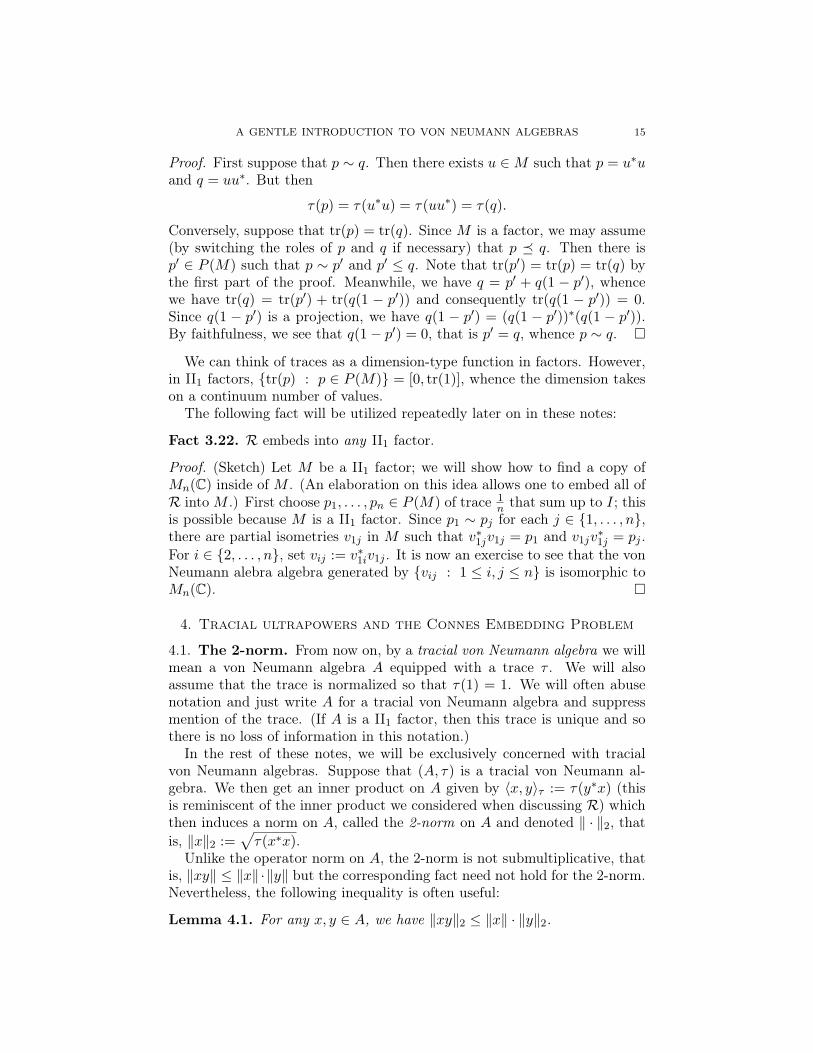
A GENTLE INTRODUCTION TO VON NEUMANN ALGEBRAS 15

Proof. First suppose that p ∼ q. Then there exists u ∈M such that p = u∗uand q = uu∗. But then

τ(p) = τ(u∗u) = τ(uu∗) = τ(q).

Conversely, suppose that tr(p) = tr(q). Since M is a factor, we may assume(by switching the roles of p and q if necessary) that p q. Then there isp′ ∈ P (M) such that p ∼ p′ and p′ ≤ q. Note that tr(p′) = tr(p) = tr(q) bythe first part of the proof. Meanwhile, we have q = p′ + q(1 − p′), whencewe have tr(q) = tr(p′) + tr(q(1 − p′)) and consequently tr(q(1 − p′)) = 0.Since q(1 − p′) is a projection, we have q(1 − p′) = (q(1 − p′))∗(q(1 − p′)).By faithfulness, we see that q(1− p′) = 0, that is p′ = q, whence p ∼ q.

We can think of traces as a dimension-type function in factors. However,in II1 factors, tr(p) : p ∈ P (M) = [0, tr(1)], whence the dimension takeson a continuum number of values.

The following fact will be utilized repeatedly later on in these notes:

Fact 3.22. R embeds into any II1 factor.

Proof. (Sketch) Let M be a II1 factor; we will show how to find a copy ofMn(C) inside of M . (An elaboration on this idea allows one to embed all ofR intoM .) First choose p1, . . . , pn ∈ P (M) of trace 1

n that sum up to I; thisis possible because M is a II1 factor. Since p1 ∼ pj for each j ∈ 1, . . . , n,there are partial isometries v1j in M such that v∗1jv1j = p1 and v1jv

∗1j = pj .

For i ∈ 2, . . . , n, set vij := v∗1iv1j . It is now an exercise to see that the vonNeumann alebra algebra generated by vij : 1 ≤ i, j ≤ n is isomorphic toMn(C).

4. Tracial ultrapowers and the Connes Embedding Problem

4.1. The 2-norm. From now on, by a tracial von Neumann algebra we willmean a von Neumann algebra A equipped with a trace τ . We will alsoassume that the trace is normalized so that τ(1) = 1. We will often abusenotation and just write A for a tracial von Neumann algebra and suppressmention of the trace. (If A is a II1 factor, then this trace is unique and sothere is no loss of information in this notation.)

In the rest of these notes, we will be exclusively concerned with tracialvon Neumann algebras. Suppose that (A, τ) is a tracial von Neumann al-gebra. We then get an inner product on A given by 〈x, y〉τ := τ(y∗x) (thisis reminiscent of the inner product we considered when discussing R) whichthen induces a norm on A, called the 2-norm on A and denoted ‖ · ‖2, thatis, ‖x‖2 :=

√τ(x∗x).

Unlike the operator norm on A, the 2-norm is not submultiplicative, thatis, ‖xy‖ ≤ ‖x‖ ·‖y‖ but the corresponding fact need not hold for the 2-norm.Nevertheless, the following inequality is often useful:

Lemma 4.1. For any x, y ∈ A, we have ‖xy‖2 ≤ ‖x‖ · ‖y‖2.

16 ISAAC GOLDBRING

Proof. We will need two standard bits of functional analysis. The first isthat in any C∗ algebra (and particular in a von Neumann algebra), we have‖yy∗‖ = ‖y‖2. Secondly, for any w ∈ A, we have w ≤ ‖w‖ · I (this followsfrom the functional calculus); consequently, if x ∈ A, then wx∗x ≤ ‖w‖x∗xsince x∗x is a positive element. We are now ready:

‖xy‖22 = τ(y∗x∗xy) = τ(yy∗x∗x) ≤ τ(‖yy∗‖x∗x) = ‖y‖2τ(x∗x) = ‖x‖22 ·‖y‖2.Note that the second equality follows from the trace property while theinequality follows from positivity and linearity.

In particular, by setting y = I, we have that ‖x‖2 ≤ ‖x‖ for all x ∈ A.

Fact 4.2. A is not complete with respect to the 2-norm. However, anyoperator norm closed and bounded subset of A is complete with respect tothe 2-norm.

We call a tracial von Neumann algebra separable if A is separable withrespect to the metric induced by the 2-norm. For example, R and L(Γ) areseparable.

4.2. Tracial ultraproducts. Operator algebraists like taking ultraprod-ucts/ultrapowers (almost) as much as model theorists do. Here is the defi-nition of the tracial ultraproduct.

Definition 4.3. Suppose that (An : n ∈ N) is a sequence of tracial vonNeumann algebras and U is a nonprincipal ultrafilter on N. Set

F((An)) := (an) ∈∏

An : supn‖an‖ <∞,

andI((An)) := (an) ∈

∏An : lim

U‖an‖2 → 0.

F and I are to remind us of the words finite and infinitesimal. It is straight-forward to check that F((An)) is an algebra and I((An)) is an operatornorm closed two-sided ideal. The quotient F((An))/I((An)) is referred toas the tracial ultraproduct of (An) with respect to U and is denoted

∏U An.

If An = A for each n, then we refer to the tracial ultraproduct as the tracialultrapower of A and denote it by AU .

Remarks 4.4.(1) Recall that if (rn) is a bounded sequence of real numbers, then

limU rn = r means, for every ε > 0, we have n ∈ N : |rn−r| < ε ∈U . It is a standard fact that the ultralimit of a bounded sequence ofreal numbers always exist.

(2) It is relatively straightforward to show that∏U An is once again a

tracial von Neumann algebra whose trace is given by tr = limU trn.Less trivially, if each An is a factor (resp. II1 factor), then so is∏U An. This will also follow from the ability to axiomatize these

concepts in (continuous) first-order logic; see Subsection 5.1.

A GENTLE INTRODUCTION TO VON NEUMANN ALGEBRAS 17

(3) The uses of ‖·‖ in F((An)) and ‖·‖2 in I((An)) is not a typo. Indeed,if one replaced ‖ · ‖2 with ‖ · ‖ in the definition of I((An)), then onewould be performing the C∗ ultraproduct; unless one is in a trivialsituation, the C∗ ultraproduct of a sequence of von Neumann alge-bras is not a von Neumann algebra again. (See [13] for a wonderfuldiscussion of this issue.)

Remark 4.5. There are two bits of notational nuances that model theoristsshould be aware of. First of all, operator algebraists like to use the notationβN \ N to denote the set of all nonprincipal ultrafilters on N. Secondly,operator algebraists like to use the notation ω for an element of βN \N; thisclearly causes confusion for logicians and we will refrain from this practice.

We will see later that the tracial ultraproduct is precisely the model-theoretic ultraproduct in an appropriate continuous logic.

4.3. The Connes Embedding Problem. In 1976, Connes proved the fol-lowing result:

Theorem 4.6. Fix U ∈ βN \ N. Then L(Fn) embeds into RU .

He then remarked that the previous fact “ought to be true for any separa-ble II1 factor.” This remark has yet to be proven and the resulting problemis known as the Connes Embedding Problem (note the use of the word “prob-lem” rather than “conjecture”). It is arguably the most important unsolvedproblem in operator algebras. It has an unbelievable number of surprisingequivalent formulations (see [3]). It also has an interesting interaction withthe model theory of tracial von Neumann algebras, as we will see a bit later.

Let us introduce some terminology that will be useful. Once the model-theoretic appartus is set up in the next section, we will see that, for U ,V ∈βN \ N and A a separable tracial von Neumann algebra, A embeds intoRU if and only if A embeds into RV . For that reason, we will say thatA is Rω-embeddable if A embeds into some (equivalently any) nonprincipalultrapower of R. (Yes, I know, I am acquiescing to the operator algebraistnotation.) Thus, the Connes Embedding Problem (which we will abbreviateCEP) asks whether every separable II1 factor is Rω-embeddable.

Fact 4.7. Any tracial von Neumann algebra embeds into a II1 factor. In-deed, if A is a tracial von Neumann algebra, then A ∗L(Z) (free product) isa II1 factor and A ⊆ A ∗ L(Z).

Thus, we may replace the word “II1 factor” by “tracial von Neumann al-gebra” in the statement of the CEP.

5. Some Model Theory of tracial von Neumann algebras

In this section, we will highlight some of the most striking aspects of themodel theory of tracial von Neumann algebras. We should remark that weare still at the early stages of our understanding of the situation. We will

18 ISAAC GOLDBRING

be brief with our discussion, referring the reader to the appropriate parts ofthe literature where these things are discussed in greater detail.

5.1. Axiomatizability. The first task is to make the tracial von Neumannalgebras the models of a theory in an appropriate logic. The approach devel-oped in [7] is to work in a version of continuous logic (a la [1]) that contains“domains of quantification.” The metric on a structure is required to be com-plete with respect to each domain of quantification and the language has tospecify a modulus of uniform continuity for the symbols on each domain.

For tracial von Neumann algebras, the metric is the one induced by the2-norm. Since the 2-norm is complete with respect to operator norm closedand bounded sets, the domains of quantification Dn correspond to the ball ofradius n around 0 with respect to the operator norm. We include a symbolfor the 2-norm, but not the operator norm. Indeed, the operator norm is notuniformly continuous with respect to the metric induced by the 2-norm andcould thus not be asked to be a distinguished predicate.

However, writing down a set of axioms that captures all of the structuresthat are the result of viewing tracial von Neumann algebras in this way istricky business. Indeed, while asking that the structure is a tracial unital∗-algebra is not so difficult, requiring that the domains Dn correspond tothe operator norm balls is difficult considering that one is not allowed torefer to the operator norm in the axioms! Nevertheless, it is shown in [7]that one can axiomatize the class of structures that are the result of viewingtracial von Neumann algebras in the way specified above. Since the classof tracial von Neumann algebras are closed under subalgebras, the resultingaxiomatization should be universal. (This was not the case in the originalversion of [7].) We will henceforth refer to the theory of tracial von Neumannalgebras in this logic as TvNa.

We should mention that verifying the correctness of the axioms for tracialvon Neumann algebras is nontrivial and uses some facts from von Neumannalgebra theory, including functional calculus, the Kaplansky density theorem,the Russo-Dye theorem, and the GNS construction.

One feature of the logic used to study tracial von Neumann algebras isthat the corresponding ultraproduct construction, when applied to tracialvon Neumann algebras, is precisely the tracial ultraproduct construction.This yields a proof of the fact that the tracial ultraproduct of a family oftracial von Neumann algebras is once again a tracial von Neumann algebra.

Since the weak closure of a union of a chain of factors is once again afactor, the class of factors should be ∀∃-axiomatizable. An explicit set of∀∃-axioms is given in [7]; proving the correctness of these axioms requiresthe Dixmier Averaging Theorem. Once again, this yields as a corollary thatthe tracial ultraproduct of a family of factors is once again a factor.

Similarly, the class of II1 factors is also ∀∃-axiomatizable. The axiom oneneeds to add to the axioms for factors in order to get the axioms for II1

A GENTLE INTRODUCTION TO VON NEUMANN ALGEBRAS 19

factors is quite easy to write down. In fact, here it is:

infx∈D1

(‖xx∗ − (xx∗)2‖2 + | tr(xx∗)− 1π|) = 0.

IfM is a II1 factor, then by the remark following Lemma 3.21, we know thatthere is a projection in M of trace 1

π , whence this projection witnesses thatM satisfies this axiom. On the other hand, suppose thatM is a tracial factorthat satisfies the above axiom but is not a II1 factor. From our discussionin Section 3.3, we see that M is thus a type In factor for some n, whenceisomorphic to Mn(C) for some n. Since D1(Mn(C)) is compact, the infaxiom is actually realized rather than approximately realized, say by a ∈D1(Mn(C)). Let p = aa∗; then p is a projection of trace 1

π . However, thetraces of projections in Mn(C) are of the form k

n for k ∈ 0, 1, . . . , n, acontradiction. (We thus see that the actual value of 1

π was not relevant, onlythat it was irrational.) Once again, we see that the tracial ultraproduct of afamily of II1 factors is once again a II1 factor.

The fact that the class of II1 factors is ∀∃-axiomatizable has a very in-teresting model theoretic consequence. Recall that a model M of a theoryT is an existentially closed model of T if for any extension N ⊇ M that isalso a model of T and any formula ϕ(x) with parameters from M , we have(infx ϕ(x))M = (infx ϕ(x))N . Since any model of TvNa extends to a II1 factor(Lemma 4.7) and the theory of II1 factors is ∀∃-axiomatizable, we see that

Proposition 5.1. Any existentially closed tracial von Neumann algebra isa II1 factor.

This proposition was the model theoretic reason for appreciating II1 fac-tors alluded to at the end of Subsection 3.2.

We should mention that we only know of one concrete example of a sepa-rable existentially closed II1 factor, namely R, although we know that thereare continuum many separable existentially closed II1 factors; see [5].

While we are on the topic of axiomatizability, let us discuss one interestingside note. In order to show thatR and L(F2) are not isomorphic, Murray andvon Neumann isolated a property of II1 factors that R has and that L(F2)does not. The property, called property (Γ), says that, for every finite tuplex and every ε > 0, there is a trace 0 unitary u such that [xi, u] := xiu− uxihas 2-norm less than ε. It turns out that property (Γ) is axiomatizable incontinuous first-order logic. Indeed, for each n ≥ 1, let σn be the sentence

supx

infy

(‖y∗y − I‖2 + |τ(y)|+n∑i=1

‖[xi, y]‖2),

where x is an n-tuple. Notice that σMn = 0 does not at first glance guaran-tee that there exists a trace 0 unitary that almost commutes with each xi,but that there is an “almost” unitary of small trace that almost commuteswith each xi (as inf’s are not necessarily realized in an arbitrary structure);however, a standard functional calculus trick allows one to move that near

20 ISAAC GOLDBRING

witness to an actual trace 0 unitary with the desired property. It followsthat a II1 factor satisfies property (Γ) if and only if it makes each σn equalto 0. As a consequence, we see that R 6≡ L(F2).

The following weaker version of Question 2.9 is still open:

Question 5.2. If m,n ≥ 2 are distinct, is L(Fm) ≡ L(Fn)?

5.2. The model theoretic version of CEP. Suppose that A is an Rω-embeddable tracial von Neumann algebra. Then, by standard model theory,we have that A |= Th∀(R). Conversely, suppose that A |= Th∀(R) is sepa-rable. Let M |= Th(R) be separable such that A embeds into M ; we maychoose M separable by Downward Löwenheim-Skolem. Then since RU is anℵ1-saturated model of Th(R), we have that M embeds into RU , whence Ais Rω-embeddable. In other words:

Lemma 5.3. If A |= TvNa is separable, then A is Rω-embeddable if and onlyif A |= Th∀(R).

Since TvNa is universally axiomatizable, we see that:

Corollary 5.4. CEP is equivalent to the statement TvNa = Th∀(R).

We should mention that, using “abstract model-theoretic nonsense,” Hart,Farah, and Sherman proved in [8] that there exists a separable II1 factorS such that TvNa = Th∀(S); they call such an S locally universal. In fact,once there exists one locally universal II1 factor, then there exists manylocally universal II1 factors, e.g. if S is locally universal, so is S ∗A for anyA |= TvNa. CEP asks whether or not R is locally universal.

5.3. Model companions and connection to CEP. Based on work ofNate Brown [2], the following appears in [9]:

Theorem 5.5. Th(R) does not have quantifier elimination.

We also noticed that the proof of the preceding theorem applied to awider class of von Neumann algebras. First, we need a definition. Call a II1factor A McDuff if A ⊗ R ∼= R. (We have not defined the tensor productof von Neumann algebras, but it works as one might guess; see [10] for moredetails.) For example, R is McDuff. Indeed, a fancier way of describingour construction of R was that R =

⊗∞n=1M2(C); it seems quite plausible

(and is in fact the truth) that the tensor product of two infinite tensorpowers of M2(C) would be isomorphic to one such infinite tensor power.More generally, if A is a II1 factor, then A embeds into a McDuff II1 factor,namely A⊗R.

Theorem 5.6. If S is locally universal and McDuff, then Th(S) does nothave quantifier elimination.

In [8], it is shown that, for separable II1 factors, being McDuff is an ∀∃-axiomatizable property. Since every II1 factor embeds into a McDuff II1factor (by tensoring with R), it follows that every existentially closed II1

A GENTLE INTRODUCTION TO VON NEUMANN ALGEBRAS 21

factor is McDuff. (On a side note, if S is locally universal, so are S ⊗R andS ∗ R; since the first is McDuff and the second is not, we see that not alllocally universal II1 factors are elementarily equivalent.)

The previous observation, combined with the fact that TvNa has the amal-gamation property, yields the following negative result:

Theorem 5.7 (G., Hart, Sinclair [9]). TvNa does not have a model compan-ion.

Proof. Suppose that Th(S) is the model companion of TvNa, where S is sepa-rable. Since Th(S) is model complete, it follows that S is existentially closed,whence a McDuff II1 factor. Moreover, since TvNa = Th∀(S), we see thatS is locally universal. On the other hand, since TvNa has the amalgamationproperty, it follows that the model companion has quantifier elimination, acontradiction.

Instead of asking for a model companion of TvNa, one might ask for a modelcomplete theory of II1 factors. This question has an interesting connectionto CEP. First, two preparatory results.

Fact 5.8. Every embedding R → RU is unitarily conjugate to the diagonalembedding. In particular, every embedding R → RU is elementary.

Exercise 5.9. Use Fact 5.8 to prove that R is the prime model of its theory.

Lemma 5.10 ([9]). IfM is an Rω-embeddable II1 factor such that Th(M) is∀∃-axiomatizable (in particular, if Th(M) is model-complete), then M ≡ R.

Proof. (Sketch) This is a “sandwiching chain” argument. To begin the ar-gument, one embeds R into M (Fact 3.22) and M into RU and uses thefact that the composition of these embeddings is elementary by Fact 5.8.One continues the chain by taking the ultrapowers of the aforementionedmaps.

Thus, the only possible ∀∃-axiomatizable complete theory of II1 factors isTh(R). It is still currently unknown whether or not Th(R) is ∀∃-axiomatizable.

Theorem 5.11. If CEP has a positive solution, then there is no model com-plete theory of II1 factors.

Proof. Suppose that Th(M) is model complete, where M is a II1 factor. ByCEP, M is Rω-embeddable, whence, by Lemma 5.10, Th(M) = Th(R). ByCEP again, we see that Th(R) is the model companion of TvNa, contradictingTheorem 5.7.

A more careful analysis led to the following sharpening of the Theorem5.11:

Theorem 5.12 (Farah, G., Hart [5]). If Th∀(R) has the amalgamationproperty, then there is no model complete theory of II1 factors.

22 ISAAC GOLDBRING

The previous result is indeed sharper than Theorem 5.11 as the fact thatTvNa has the amalgamation property shows that CEP implies that Th∀(R)has the amalgamation property. In fact, in [5], we exhibit a concrete Rω-embeddable tracial von Neumann algebra such that the ability to amalga-mate over it while staying Rω-embeddable yields the fact that there is nomodel complete theory of II1 factors.

5.4. Stability. A major impetus for understanding the model theory of tra-cial von Neumann algebras stemmed from many questions of the form: “Howcanonical are tracial ultraproducts and ultrapowers” For example, if M is aseparable tracial von Neumann algebra and U ,V ∈ βN \ N, is MU ∼= MV?(There were many variants of this questions asked by many different peo-ple, but let us focus on this particular question.) Now, if the continuumhypothesis holds, then MU and MV are saturated elementarily equivalentstructures of the same uncountable density character. Thus, a familiar backand forth argument shows that they are isomorphic. Thus, the question isonly interesting if we assume the negation of the continuum hypothesis.

The following theorem (in its classical form) is model-theoretic folklore,but a proof can be found in [7]:

Theorem 5.13. Suppose that the continuum hypothesis fails and M is aseparable structure in a countable language. Then the following are equiva-lent:

(1) For every U ,V ∈ βN \ N, we have MU ∼= MV .(2) Th(M) is stable.

A word about the proof: the direction (1) ⇒ (2) proceeds by showingthat a witness to the order property allows one to encode the partial or-der on increasing sequences of natural numbers (modulo almost everywhereagreement) by almost everywhere domination into the structure and thenuse the fact that there are nonprincipal ultrafilters whose associated partialorders have distinct coinitalities (a result due independently to Dow andShelah). The other direction proceeds by showing that stability still allowsone to conclude that MU is saturated: one realizes a type over a large set byfinding Morley sequences for its restriction to a countable set of size contin-uum in MU and then using some forking calculus and statonarity of typesto find an actual realization of the original type.

Suppose that M is a II1 factor. By Fact 3.22, one can find arbitrarilylarge matrix algebras in M . A straightforward computation with matricesallows one to find an order in M , whence II1 factors are unstable and hencehave nonisomorphic ultrapowers (assuming the negation of the continuumhypothesis). Similar reasoning allows one to show that there are nonisomor-phic ultraproducts of matrix algebras. (Details for these two facts can befound in [6].)

Which tracial von Neumann algebras are stable? That question is alsoanswered in [6]:

A GENTLE INTRODUCTION TO VON NEUMANN ALGEBRAS 23

Theorem 5.14 (Farah, Hart, Sherman). If M |= TvNa, then M is stable ifand only if it is of type I.

A word is in order about the statement of Theorem 5.14. We only definedthe type classification for factors, but there is also a type classification forarbitrary von Neumann algebras. We will not explain this in detail, but onlysay as much as is needed to understand the previous result. A tracial vonNeumann algebra M can be written M = MII1 ⊕MI2 ⊕MI3 ⊕ · · · , wherethe subscript tells us the type of the algebra. A type In A algebra is of theform Mn(C) ⊗ Z(A) and M as above is said to be of type I if its type II1component is 0.

A word about the proof of Theorem 5.14. If M is not of type I1, thenby our earlier discussion, M is unstable. It remains to show that type Ialgebras are stable; equivalently, we show that all ultrapowers of type I al-gebras are isomorphic. It can be shown that ultrapowers and direct sums“commute”, so it suffices to show that ultrapowers of type In algebras are iso-morphic. It can be shown that (Mn(C)⊗Z(A))U ∼= Mn(C)U⊗Z(A)U . Since(Mn(C))U ∼= Mn(C) (compact things are isomorphic to their ultrapowers),it suffices to show that the ultrapowers of abelian von Neumann algebras areall isomorphic. There are many ways to explain this, but perhaps the easiestis to recall that there is an equivalence of categories between the category ofabelian von Neumann algebras and the category of atomless probability al-gebras, respecting the ultraproduct construction; the latter theory is knownto be stable (see [1]), finishing the proof of the thoerem.

References

[1] I. Ben Yaacov, A. Berenstein, C. W. Henson, A. Usvyatsov, Model theory for metricstructures

[2] N. Brown, Topological dynamical systems associated to II1 factors, Adv. Math. 227(2011), 1665-1699.

[3] V. Capraro, A survey on Connes’ embedding conjecture, arXiv 1003.2076.[4] J. Conway, A course in functional analysis, GTM 96.[5] I. Farah, I. Goldbring, B. Hart, Amalgamating, Rω-embeddable II1 factors, note avail-

able at http:///www.math.uic.edu/ isaac[6] I. Farah, B. Hart, D. Sherman, Model theory of operator algebras I: Stability, to appear

in the Bulletin of the London Mathematical Society.[7] I. Farah, B. Hart, D. Sherman, Model theory of operator algebras II: Model theory,

preprint.[8] I. Farah, B. Hart, D. Sherman, Model theory of operator algebras III: Elementary

equivalence and II1 factors, preprint.[9] I. Goldbring, B. Hart, T. Sinclair, The theory of tracial von Neumann algebras does

not have a model companion, to appear in the Journal of Symbolic Logic.[10] V. Jones, Von Neumann algebras, lecture notes from his webpage.[11] M. Lupini and A. Tornquist, Set theory and von Neumann al-

gebras, lecture notes from Appalachian set theory. Available athttp://www.math.cmu.edu/ eschimme/Appalachian/AsgerMartino.pdf

[12] J. Lurie, Course notes on von Neumann algebras, available athttp://www.math.harvard.edu/ lurie/

24 ISAAC GOLDBRING

[13] V. Pestov, Hyperlinear and sofic groups: a brief guide, Bull. Symb. Logic, 14, Number4 (2008).

Department of Mathematics, Statistics, and Computer Science, Universityof Illinois at Chicago, Science and Engineering Offices M/C 249, 851 S.Morgan St., Chicago, IL, 60607-7045

E-mail address: isaac@math.uic.eduURL: http://www.math.uic.edu/~isaac