Introduction · Web viewEach statistical process: Starts with sending the request file with...

Table Structure Definitions and Queriesfor SDMX Data

Prepared by: Jan Kaczanowski

Reviewed by: Maria Leopold

Contact person:

Jan Kaczanowski, e-mail: [email protected]

Department of Statistics

Narodowy Bank Polski

Świętokrzyska 11/21, 00-919 Warszawa, Poland

1

mailto:[email protected]

Spis treściI. Introduction...................................................................................................4

I.1. Explanation of applied description rules and symbols............................6II. Overview of Table Definition Structures......................................................7

II.1. SDMX identification of unique observation.........................................7II.2. Statistical data and metadata business processes...................................8II.3. Request Data Table..............................................................................10II.4. Result Data Table................................................................................12II.5. Identification of the group of SDMX observations for the same date.13II.6. Table Definition Query........................................................................15

III. SDMX formula notations...........................................................................19III.1. SDMX date formulas...........................................................................19III.2. SDMX transformation formula notation............................................22III.3. Notation of Validation Rules...............................................................27

IV. The Table Definitions and Fields...............................................................29IV.1. Mapping of table to xml elements.......................................................29IV.2. Different types of table fields..............................................................31

IV.2.1. Field <EMPTY>............................................................................31IV.2.2. Field <CAPTION>.........................................................................32IV.2.3. Field <LABEL>.............................................................................32IV.2.4. Field <DATE>...............................................................................33IV.2.5. Field <CELL>................................................................................34IV.2.5. Element <OBS_VAR> belonging to <CELL> field......................36

IV.3. The functionality of <CELL> element................................................37IV.3.1. Simple Example.........................................................................37IV.3.1. Complicated Example................................................................39

IV.4. The xml structure of Request Data Table (simple case)......................44IV.5. The xml structure of Result Data Table (simple case)........................47IV.6. The xml structures of Request and Result Data Table (complicated case). 51

V. SDMX Table Definition Query...................................................................55

2

V.1. Introduction.........................................................................................55V.2. Simple example of Table Definition Query........................................55

VI. Application for processing of Table Definition Queries............................79VI.1. Prototype application...........................................................................79VI.2. Instruction for running of the application............................................79VI.3. List of files...........................................................................................83

3

I. Introduction

SDMX is widely used standard for exchanging of statistical data by Central Banks, National Statistical Offices and International Statistical Institutions.

The current version SDMX standard solves two problems: exchange of statistical data messages and supplies method for systematic time series classification.

The new challenges for SDMX standard are effective production of statistical information and user-friendly presentation of SDMX statistical data.

There were elaborated three new xml structures for SDMX data presentation and statistical information production:

1) Request Data Table The business task of Request Data Table is user-friendly presentation of requirements for SDMX data.The Request Data Table is a xml structure containing the following information:

- template of table for data presentation, - requirements for SDMX data, - transformation formulas and validation rules.

2) Result Data TableIts business functionality is user-friendly presentation of statistical SDMX data and calculated economic indicators.The Result Data Table is a xml structure containing the following information:

- template of table for data presentation, - values of SDMX data and calculated values of economic

indicators,- transformation formulas and validation rules.

3) Table Definition QueryIts business purpose is effective statistical information production.The Table Definition Query is a xml compact structure containing all necessary information for creating:

- Request Data Table- Result Data Table.

The advantage of newly developed solution is based on integration of the following features:

- SDMX data identification,

4

- user-friendly presentation of statistical data and metadata,- transformation formulas, - validation rules,- method of effective statistical information production:

SDMX data base querying.

It is proposed to include newly developed structures (Table Definition Queries, Request Data Table and Result Data Table) in a new version of SDMX standard.

5

I.1. Explanation of applied description rules and symbols.

All examples presented in the paper are based on SDMX statistical data imported from Statistical Data Warehouse of European Central Bank. There are used the same time series identifiers as in Statistical Data Warehouse ECB.

The names of xml elements are marked in the text as follow:

<Element_Name>

where “Element_Name” means element name.

The names of xml attributes are marked in the text as follow:

@Attribute_Name

where “Attribute_Name” means attribute name.

The names of SDMX parameters and date parameters are marked in the xml structure in the following way:

[?Parameter_Name?]

where “Parameter_Name” means parameter name.

6

II. Overview of Table Definition Structures.

II.1. SDMX identification of unique observation.

A Time Series is a series of observations collected according to some frequency of dates. An Observation is a value of a statistical indicator measured in a given date.

The important achievement of SDMX standard is development of a method for systematic classification of Time Series.

Therefore multidimensional identifier of Time Series identifies univocally Time Series. In order to identify univocally the observation two parameters are necessary:

1) SDMX Time Series Identifier,2) Date of the observation.

Thus the request for observation should contain these two parameters.

For example request for the value of Gross Domestic Product of Poland in market prices for 2016 year contains:

1) SDMX Time Series IdentifierMNA.A.N.PL.W2.S1.S1.B.B1GQ._Z._Z._Z.EUR.V.N

2) Date2016-12-31

and as a result of the request one gests value of observation equal:

424.269 billion Euro

Such method of request for SDMX observation values is used by SDMX Web-Services RestFul technology.

The method of request for observation value and next getting feedback with result value of observation is a crucial procedure for processing of Structure Table Definitions and Queries.

7

II.2. Statistical data and metadata business processes.

There are three main types of statistical data business processes:

1) Data Collection.When the International Organization sends the request with requirements for SDMX statistical data to State Institution and next gets feedback in the form of the SDMX file with data.

2) Data Transformation.When the administrator of the data calculates from existing SDMX data new SDMX data and save the results into SDMX data base (for example new economic indicator).

3) Data Retrieving from Statistical Data Base.When the end-user (economist) retrieves from SDMX Data Base the data, calculates economic indicators and presents the results in the ad-hoc designed table.

1) Statistical Data Collection (from State Institutions)

2) Statistical Data Transformation (calculation of new Time Series from existing data in DB)

3) Statistical Data Retreiving (production of report tables)

InternationalOrganization

State StatisticalInstitution

RequirementsResult: SDMX data file

User Economist

SDMXDate Base

Requirements

Result: SDMX data file

Admin SDMXDate Base

SDMXDate Base

Requirements Result: SDMX data file

SDMXDate Base

Figure 1. Schema of the main statistical data business processes.

Each statistical process:

1) Starts with sending the request file with requirements for data,2) Ends with receiving the result file with data.

Therefore it would be worthy to elaborate SDMX structures for:

1) Sending the request 2) Receiving the result.

8

The proposed SDMX structures for these purposes are:

1) Request Data Table for sending the requirements for data,2) Result Data Table for receiving the statistical results.

The overview of proposed above structures is described in chapters II.3 and II.4 and the more detail information are in chapters III and IV.

The very important SDMX process is:

- Statistical Information Production.

Statistical information production means creating the reports containing tables based on SDMX data from large SDMX data warehouses.

The Statistical Information consists of the following components:

- requirements for SDMX data,- formulas for calculation of economic indicator,- validation rules for values of calculated formulas,- templates for the statistical data presentation.

The process of statistical information production should be transparent, effective and user-friendly.

Therefore there is a demand to develop metadata structure integrating above mentioned components.

The Table Definition Query is a xml compact structure containing all necessary information for creating:

- Request Data Table- Result Data Table.

The advantage of the Table Definition Query structure is its compactness. Thus it is possible to create and modify its manually.

The overview of the structures is described in chapters II.5 and II.6 and the detail information are in chapter V.

9

II.3. Request Data Table.

The Request Data Table is an xml structure containing requirements for import of SDMX data and for transformation of SDMX data which is prepared for visualization in the table.

The requirements for the data are sent very often in the form of table with cells marked by SDMX Time Series Identifiers. The simple example of such table is presented in fig.2.

Credit (Resources) Debit (Uses) Balance (Credits minus Debits)DATE_BASE DATE_BASE DATE_BASE

Current account BP6.M.N.PL.W1.S1.S1.T.C.CA._Z._Z._Z.EUR._T._X.N BP6.M.N.PL.W1.S1.S1.T.D.CA._Z._Z._Z.EUR._T._X.N BP6.M.N.PL.W1.S1.S1.T.B.CA._Z._Z._Z.EUR._T._X.NGoods BP6.M.N.PL.W1.S1.S1.T.C.G._Z._Z._Z.EUR._T._X.N BP6.M.N.PL.W1.S1.S1.T.D.G._Z._Z._Z.EUR._T._X.N BP6.M.N.PL.W1.S1.S1.T.B.G._Z._Z._Z.EUR._T._X.NServices BP6.M.N.PL.W1.S1.S1.T.C.S._Z._Z._Z.EUR._T._X.N BP6.M.N.PL.W1.S1.S1.T.D.S._Z._Z._Z.EUR._T._X.N BP6.M.N.PL.W1.S1.S1.T.B.S._Z._Z._Z.EUR._T._X.NPrimary income BP6.M.N.PL.W1.S1.S1.T.C.IN1._Z._Z._Z.EUR._T._X.N BP6.M.N.PL.W1.S1.S1.T.D.IN1._Z._Z._Z.EUR._T._X.N BP6.M.N.PL.W1.S1.S1.T.B.IN1._Z._Z._Z.EUR._T._X.NSecondary income BP6.M.N.PL.W1.S1.S1.T.C.IN2._Z._Z._Z.EUR._T._X.N BP6.M.N.PL.W1.S1.S1.T.D.IN2._Z._Z._Z.EUR._T._X.N BP6.M.N.PL.W1.S1.S1.T.B.IN2._Z._Z._Z.EUR._T._X.N

DATE_BASE 2016-06-30

Current Account BOPmln. EUR

Figure 2. Request Data Table for data collection process of current account and its main components (monthly).

In practice the request for data is sent often in the form of Excel tables. Such tables are very useful because they contain user-friendly presentation of requirements (in the form of table) and are easy to operate by IT tools.

This type presentation of SDMX data requirements has been practiced by ECB and Eurostat for more than ten years.

The header and lateral cells of the table contain descriptions. The cells inside the table contain SDMX Time Series Identifiers. Additionally it is given the date for the requested data.

The request for one cell value consists of two parameters:

1) Time Series Identifier of the cell2) Date of the table.

In a given above example the request for the cell observation of “Goods, Credit for Jun 2016” (yellow marked cell) contains two attributes:

1) Time Series Identifier equal BP6.M.N.PL.W1.S1.S1.T.C.G._Z._Z._Z.EUR._T._X.N

2) Date for all observations is equal “2016-06-31”

These parameters univocally define the request for observation value. The table could be filled with the data values (for identified observations).

10

Date of requested data

Time Series Identifier

However, there are several disadvantages of such specification of requirements for SDMX data:

1) it is limited to Ms Excel tool,2) it does not comply with SDMX standard.

Therefore it is a demand for the xml-structure with functionality:

user-friendly specification of request for SDMX data.

The newly designed xml-structure is called Request Data Table and covers the following information:

- template of the table,- requirements for SDMX data, - transformation formulas and validation rules.

The xml structure should be prepared for presentation in internet, loading to Excel and printing in PDF.

The xml-structure was built by mapping presentation table fields into xml-elements and its features into attributes. The detail description of xml structure of Request Data Table will be given later.

The simplified example of mapping cell containing request for “Goods for Credit of Jun 2016” (cell marked with yellow) to xml is presented below:<CELL TS_TEMP="BP6.M.N.PL.W1.S1.S1.T.C.G._Z._Z._Z.EUR._T._X.N" FORMULA="_C14" >

<OBS_VAR OBS_ID="_C14" TS_TEMP=" BP6.M.N.PL.W1.S1.S1.T.C.G._Z._Z._Z.EUR._T._X.N" DATE_VAL="2016-06-30"/>

</CELL>The parameters of observation variable <OBS_VAR> are following:

1) Time Series Identifier in attribute @TS_TEMP1 BP6.M.N.PL.W1.S1.S1.T.C.G._Z._Z._Z.EUR._T._X.N

1) Date of observation equal in attribute @DATE_VAL“2016-06-31”

The SDMX Time Series Identifier identifies univocally the time series and the date parameter univocally observation.

The attribute @OBS_ID is an identifier of observation. In the current example the attribute @FORMULA is equal “_C14” points the observation variable <OBS_VAR> element with @OBS_ID attribute equal “_C14” . By

1 The xml attributes are marked in text by “@”.

11

substitution in formula the variable “_C14” with pointed observation value one gets the value of cell.

II.4. Result Data Table.

The Result Data Table is an xml structure designed for easy visualization in form of table the SDMX data values and calculated economic indicators.

The Excel table containing requirements for SDMX could be filled with the data by the data supplier. In the cells for dates are presented values of dates. The cells with Time Series Identifiers are filled by observation values relevant to Time Series Identifiers and date of the table (DATE_BASE). The example is presented below.

Credit (Resources) Debit (Uses) Balance (Credits minus Debits)2016-06-30 2016-06-30 2016-06-30

Current account 20427 21144 -717Goods 15185 14548 637Services 3818 2490 1328Primary income 1020 3704 -2685Secondary income 404 402 2


Figure 3. The feedback of Request Data Table filled with data is called Result Data Table. The current account for Poland monthly.

The presentation of data is user-friendly and easy to use because it is in Excel. Unfortunately it has some disadvantages (similar to mentioned in previous chapter):

1) it is limited to Ms Excel tool,2) it does not comply with SDMX standard.

In order to overcome these disadvantages the new xml-structure called Result Data Table was designed. The new structure contains the following information:

- template of the table,- transformation formulas and validation rules,- SDMX values and dates values.

The xml structure is well prepared for presentation in internet, for loading to Excel and printing in PDF.

12

The xml-structure of Result Data Table is pretty similar to Request Data Table. The main difference is that the Result Data Table contains not only formulas and metadata but also values of dates, values of observations and values of calculated economic indicators.

Here is presented simplified example of mapping cell containing result value for “Current Account for Credit for Jun 2016” (cell marked with yellow in fig.3) to xml: <CELL TS_TEMP="BP6.M.N.PL.W1.S1.S1.T.C.G._Z._Z._Z.EUR._T._X.N" FORMULA="_C14" DATE_VAL="2016-06-30" CELL_VAL="15185" OBS_CONF="F">

<OBS_VAR OBS_ID="_C14" TS_TEMP="BP6.M.N.PL.W1.S1.S1.T.C.G._Z._Z._Z.EUR._T._X.N" DATE_VAL="2016-06-30" OBS_VAL="15185"/>

</CELL>The detail description of xml structure of Result Data Table will be described later.

II.5. Identification of the group of SDMX observations for the same date

The idea of sub-set of codes was developed for RestFul notation. In order to use the sub-set of codes in Table Definition Queries structures the sub-sets should get names.

The group of observations for the same date is identified by the list of SDMX Time Series Identifiers.

For example 7 observations of Balance of Payment Current Account for Credit in Euro for December 2016 for countries :

Germany, France, Poland, Spain, Italy, Netherlands, Romania are identified by Time Series Identifiers:

BP6.M.N.DE.W1.S1.S1.T.C.CA._Z._Z._Z.EUR._T._X.NBP6.M.N.FR.W1.S1.S1.T.C.CA._Z._Z._Z.EUR._T._X.NBP6.M.N.PL.W1.S1.S1.T.C.CA._Z._Z._Z.EUR._T._X.NBP6.M.N.ES.W1.S1.S1.T.C.CA._Z._Z._Z.EUR._T._X.NBP6.M.N.IT.W1.S1.S1.T.C.CA._Z._Z._Z.EUR._T._X.NBP6.M.N.NL.W1.S1.S1.T.C.CA._Z._Z._Z.EUR._T._X.NBP6.M.N.RO.W1.S1.S1.T.C.CA._Z._Z._Z.EUR._T._X.N

13

and one date 2016-12-31.

In SDMX Web-Services RestFul notation such group of time series identifiers could be presented by the string:

BP6.M.N./

DE+FR+PL+ES+IT+NL+RO

/.W1.S1.S1.T.C.CA._Z._Z._Z.EUR._T._X.N

where

/DE+FR+PL+ES+IT+NL+RO/ is sub-set of code list CL_AREA_EE.

The following notation could be modified by adding named parameter

“PAR_1”:

BP6.M.N.[?PAR_1?].W1.S1.S1.T.C.CA._Z._Z._Z.EUR._T._X.N

where

PAR_1 - name of parameter which should be substituted by the codes DE, FR, PL,ES, IT, NL, RO,

[? parameter name ?] – the square bracket and question mark means that inside is a parameter

The list of SDMX codes which could be substituted for [?PAR_1?] consists of :

DE, FR, PL, ES, IT, NL, RO. The above described notation with parameter is very useful for Table Definitions Queries.

The group SDMX Time Series Identifiers can be constructed using not only one parameter but two or more parameters and each parameter should have relevant sub-set of SDMX codes. The above presented group of time series could be extended from Time Series for Credit to Time Series for Credit, Debit and Balance.

In Web-Services RestFul notation such extended group of time series identifiers could be presented by the formula:

BP6.M.N./DE+FR+PL+ES+IT+NL+RO/.W1.S1.S1.T.

/C+D+B/.CA._Z._Z._Z.EUR._T._X.N

where

/C+D+B/ is the second sub-set of codes from SDMX code list.

The notation with named sub-sets [?PAR_1?] and [?PAR_2?] looks like:14

BP6.M.N.[?PAR_1?].W1.S1.S1.T.[?PAR_2?].CA._Z._Z._Z.EUR._T._X.N

where

PAR_1 - name of parameter which should be substituted by DE, FR, PL,

ES, IT, NL, RO

PAR_2 - name of parameter which should be substituted by C,D,B.

The above presented notation is relevant to the table presented in fig.1.

Also date could be a parameter and in such case the notation of date parameter is following:

[?Date_1?]

where

Date_1 – name of date parameter

[?Date_1?] – the square bracket and question mark means that it is a parameter

and the parameter [?Date_1?] should be substituted by list of relevant dates.

The SDMX Web-Service RestFul notation is very useful and very well designed but this notation is not prepared for the named parameters. The named parameters are necessary for notation of Table Definition Queries. This is the reason that modification of RestFul notation has been introduced.

II.6. Table Definition Query.

Usually Request Data Table (or Result Data Table) consists of several rows and columns. Therefore the number of fields in table could range from 10 to 150 or more. Very often the data fields of table contain the economic indicators which are calculated by substitution several values of observations. The number of required observations for calculation of one economic indicator could range from 1 up to 10 or more. And each observation variable contains several parameters.

Therefore the xml-structure which contains the Request Table Structure could contain about 1000 xml elements with 5000 xml attributes. The xml-structure for Result Data Table could contain about 1000 elements and about 7000 attributes.

15

Thus preparing such complicated xml-structures manually is very cumbersome.

In order to overcome the problem the compact xml notation of table was elaborated. The new structure is called Table Definition Query. The inspiration for the idea of Table Definition Queries was taken from SQL (Structure Query Language).

The Request Data Table presented in fig. 2 consists of 15 time series belonging to Balance of Payment Key Family.

The general formula for these 15 time series could be presented by the following notation:

TS_TEMP="BP6.M.N.PL.W1.S1.S1.T.[?COLS_1?].[?ROWS_1?]._Z._Z._Z.EUR._T._X.N"

with two parameters:

[?COLS_1?] – which can take one value from the sub-set of codes from code

list CL_ACCOUNT_ENTRY:

C – Credit(Resources)D – Debit(Uses)B – Balance(Credits-Debits)

[?ROWS_1?] – which can take one value from the sub-set of codes from code list CL_ACCOUNTS_ITEM:

CA - Current Account BOPG – GoodsS – ServicesIN1- Primary incomeIN2 - Secondary income

Therefore it is possible to prepare table where in columns are different values of sub-set [?COLS_1?] and in rows are different values of sub-set [?ROWS_1?]. The table could be defined by the Table Definition Query where element <LABEL_LIST DESC_ID="BOP_ENTRY" CL_LIST="CL_ACCOUNT_ENTRY" >contains list of values of Account Entry (“C”, “D”,”B”)

and<LABEL_LIST DESC_ID="BOP_ITEM" CL_LIST="CL_ACCOUNTS_ITEM">contains the list of values of BOP items (“CA,”G”,”S”,”IN1”,”IN2”).

16

The first label list is spread over for columns and second label list is spread over rows. <SELECT> <FOR_COLUMNS> <CAPTION DESC_VAL ="Current Account BOP" > <CAPTION DESC_VAL="mln. EUR" > <SPREAD_OVER_LABELS DIM_ID="COLS_1" TYPE="DEF_DESC" DESC_ID="BOP_ENTRY"> <SPREAD_OVER_DATES DIM_DATE_ID="COLS_3">

<CELL TS_TEMP="BP6.M.N.PL.W1.S1.S1.T.[?COLS_1?].[?ROWS_1?]._Z._Z._Z.EUR._T._X.N" DATE_ID="[?COLS_3?]"

FORMULA="_C14"><OBS_VAR OBS_ID="_C14" TS_TEMP="BP6.M.N.PL.W1.S1.S1.T.[?COLS_1?].[?ROWS_1?]._Z._Z._Z.EUR._T._X.N" DATE_FORM="[?DATE_CELL?]" />

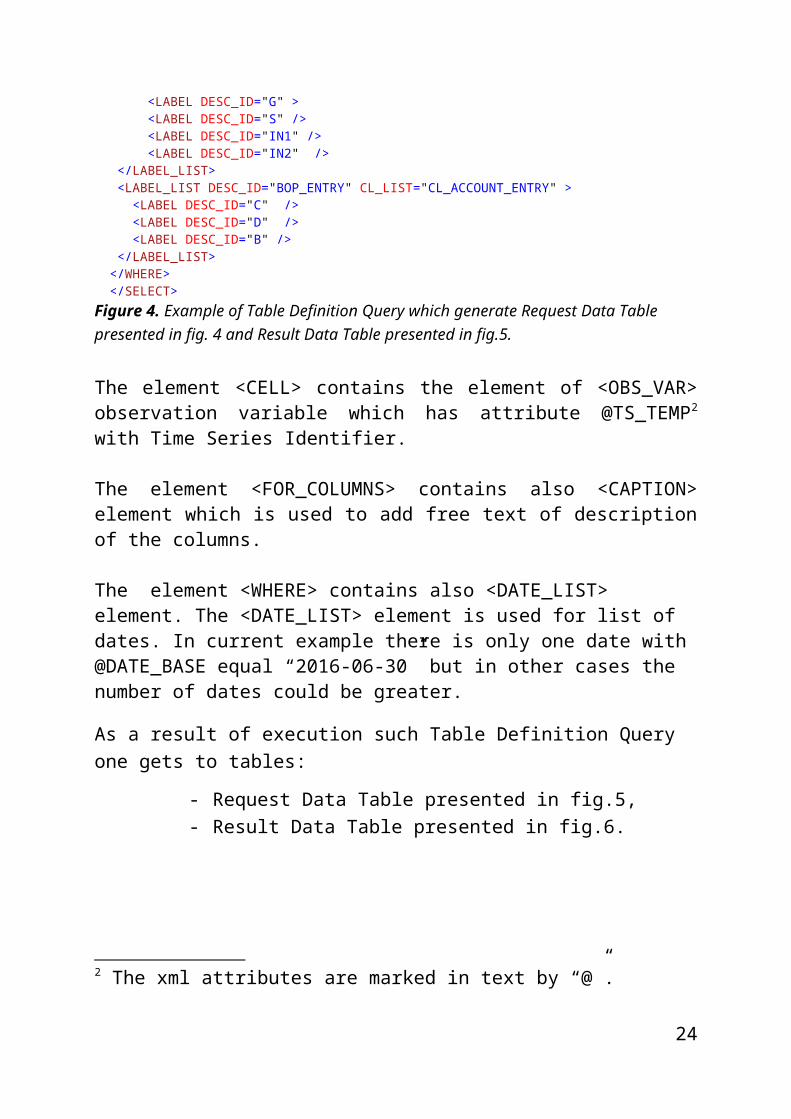
</CELL> </SPREAD_OVER_DATES> </SPREAD_OVER_LABELS> </CAPTION> </CAPTION> </FOR_COLUMNS> <FOR_ROWS> <SPREAD_OVER_LABELS DIM_ID="ROWS_1" TYPE="DEF_DESC" DESC_ID="BOP_ITEM"> </SPREAD_OVER_LABELS></FOR_ROWS> <WHERE> <DATE_LIST DATE_BASE="2016-06-30"> <DATE DATE_FORM="[?DATE_BASE?]" /> </DATE_LIST> <LABEL_LIST DESC_ID="BOP_ITEM" CL_LIST="CL_ACCOUNTS_ITEM"> <LABEL DESC_ID="CA" /> <LABEL DESC_ID="G" > <LABEL DESC_ID="S" /> <LABEL DESC_ID="IN1" /> <LABEL DESC_ID="IN2" /> </LABEL_LIST> <LABEL_LIST DESC_ID="BOP_ENTRY" CL_LIST="CL_ACCOUNT_ENTRY" > <LABEL DESC_ID="C" /> <LABEL DESC_ID="D" /> <LABEL DESC_ID="B" /> </LABEL_LIST> </WHERE> </SELECT>Figure 4. Example of Table Definition Query which generate Request Data Table presented in fig. 4 and Result Data Table presented in fig.5.

The element <CELL> contains the element of <OBS_VAR> observation variable which has attribute @TS_TEMP2 with Time Series Identifier.

The element <FOR_COLUMNS> contains also <CAPTION> element which is used to add free text of description of the columns.

The element <WHERE> contains also <DATE_LIST> element. The <DATE_LIST> element is used for list of dates. In current example there is only 2 The xml attributes are marked in text by “@”.

17

one date with @DATE_BASE equal “2016-06-30” but in other cases the number of dates could be greater.

As a result of execution such Table Definition Query one gets to tables:

- Request Data Table presented in fig.5,- Result Data Table presented in fig.6.





Figure 5. Request Data Table of current account and its main components (as presented in fig.2).




Figure 6. The feedback of Request Data Table filled with data called Result Data Table (as presented in fig.3).

Both tables were briefly described in the chapter II.

18

III. SDMX formula notations.

III.1. SDMX date formulas.

The relative date to the input date is value of date shifted by defined period.

There are economic indicators which are calculated on the basis of several observations of different time series and for different dates. Thus there is a need to introduce the notation of the formulas for calculation relative dates.

Let imagine the input date value is 2015-12-31. Below is presented notation of formulas to calculate the relative date shifted by a defined period. The value of time period could be expressed as a sum of years, quarters, months and days.

For the presented examples the input date saved in attribute @DATE_BASE was

DATE_BASE="2015-12-31"

Examples of relative date formulas and calculated result dates are presented below:

1) adding 1 year to date baseDATE_FORM="[?DATE_BASE?]+1*Y"

the calculated date value is DATE_VAL="2016-12-31"

2) subtracting 1 year to date baseDATE_FORM="[?DATE_BASE?]-1*Y


3) adding 2 quarters to date baseDATE_FORM="[?DATE_BASE?]+2*Q


4) subtracting 2 quarters from date baseDATE_FORM="[?DATE_BASE?]-2*Q


5) adding 5 months to date baseDATE_FORM="[?DATE_BASE?]+5*M


6) subtracting 5 months from date baseDATE_FORM="[?DATE_BASE?]-5*M

the calculated date value is

19

DATE_VAL="2015-07-31"7) adding 5 days from date base (this notation hasn’t been yet introduced in

prototype program for Table Definition Queries)DATE_FORM="[?DATE_BASE?]+5*D


and more complicated formulas

8) adding 1 year and 2 quarters to date baseDATE_FORM="[?DATE_BASE?]+1*Y+2*Q"


9) subtracting 2 years and adding 1 quarter to date baseDATE_FORM="[?DATE_BASE?]-2*Y+1*Q"


10) subtracting 2 years and adding 5 months to date baseDATE_FORM="[?DATE_BASE?]-2*Y+5*M"


By applying such notation the dates could be defined by formulas with one input date value substituted for [?DATE_BASE?].

Below is presented <DATE_LIST> element which contains elements <DATE>. The <DATE> element has two attributes:

@DATE_FORM – formula for date calculation,

@DATE_VAL – date value.

The <DATE_LIST> defined by the formulas where date base value is equal 2015-12-31 (@DATE_BASE attribute in xml):<DATE_LIST DATE_BASE="2015-12-31"><DATE DATE_FORM="[?DATE_BASE?]-4*Y" /><DATE DATE_FORM="[?DATE_BASE?]-3*Y" /><DATE DATE_FORM="[?DATE_BASE?]-2*Y" /><DATE DATE_FORM="[?DATE_BASE?]-1*Y" /><DATE DATE_FORM="[?DATE_BASE?]" /><DATE DATE_FORM="[?DATE_BASE?]+2*Q" /></DATE_LIST>and when the formulas are calculated<DATE_LIST DATE_BASE="2015-12-31"><DATE DATE_FORM="[?DATE_BASE?]-4*Y" DATE_VAL="2011-12-31"/><DATE DATE_FORM="[?DATE_BASE?]-3*Y" DATE_VAL="2012-12-31"/><DATE DATE_FORM="[?DATE_BASE?]-2*Y" DATE_VAL="2013-12-31"/><DATE DATE_FORM="[?DATE_BASE?]-1*Y" DATE_VAL="2014-12-31"/><DATE DATE_FORM="[?DATE_BASE?]" DATE_VAL="2015-12-31"/><DATE DATE_FORM="[?DATE_BASE?]+2*Q" DATE_VAL="2016-06-30"/></DATE_LIST>

20

The same list could be used for another value of date base value 2012-12-31 (@DATE_BASE attribute in xml):<DATE_LIST DATE_BASE="2012-12-31"><DATE DATE_FORM="[?DATE_BASE?]-4*Y" /><DATE DATE_FORM="[?DATE_BASE?]-3*Y" /><DATE DATE_FORM="[?DATE_BASE?]-2*Y" /><DATE DATE_FORM="[?DATE_BASE?]-1*Y" /><DATE DATE_FORM="[?DATE_BASE?]" /><DATE DATE_FORM="[?DATE_BASE?]+2*Q" /></DATE_LIST>and when the formulas are calculated<DATE_LIST DATE_BASE="2012-12-31"><DATE DATE_FORM="[?DATE_BASE?]-4*Y" DATE_VAL="2008-12-31"/><DATE DATE_FORM="[?DATE_BASE?]-3*Y" DATE_VAL="2009-12-31"/><DATE DATE_FORM="[?DATE_BASE?]-2*Y" DATE_VAL="2010-12-31"/><DATE DATE_FORM="[?DATE_BASE?]-1*Y" DATE_VAL="2011-12-31"/><DATE DATE_FORM="[?DATE_BASE?]" DATE_VAL="2012-12-31"/><DATE DATE_FORM="[?DATE_BASE?]+2*Q" DATE_VAL="2013-06-30"/></DATE_LIST>The presented date formulas give a hint for creating lists of date values calculated according to some rules with one input date given in attribute @DATE_BASE.

21

III.2. SDMX transformation formula notation.

The transformation formula is a formula for calculation of new Time Series’ observation taking as an input existing Time Series’ observations.

Economic indicators are applied for quantitative presentation of some economic phenomenon. The important economic indicators are stored in data base as new Time Series. The calculation of new Time Series using the observations from existing Time Series is called transformation formula or transformations.

The transformations are very often performed by statisticians and economists. Thus there is a demand for the notation of transformation formulas in SDMX Standard.

The example of such indicator is International Investment Position Net Value presented as a percentage of Gross Domestic Product. In order to perform the calculation one should apply the following formula:

FORMULA="(_C14/(_A11+_A12+_A13+_A14))*100"

where

_C14 – is an observation variable identifier containing value of International Investment Position Net Value in Euro in the end of the one year period,

_A11 – is an observation variable identifier containing Gross Domestic Product in Euro for 1 quarter,



_A14 – is an observation variable identifier containing Gross Domestic Product in Euro for 4 quarter._A11+_A12+_A13+_A14

The sum of Gross Domestic product for sequence of four quarters gives the Gross Domestic Product for one year.

22

Below is presented example of calculation of such economic indicator for Germany for 2013-12-31.

Here is formula and calculated resultFORMULA="(_C14/(_A11+_A12+_A13+_A14))*100" CELL_VAL="34.3492"

and below are observations values identified by the symbols: OBS_ID="_A11" OBS_VAL="685460.00"

OBS_ID="_A12" OBS_VAL="698330.00"

OBS_ID="_A13" OBS_VAL="723160.00"

OBS_ID="_A14" OBS_VAL="719290.00"

OBS_ID="_C14" OBS_VAL="970792"

The above presented notation of the formula could be generalized for any date of the formula:FORMULA

two parameters time series identifier of output value and formula for calculation of date with input value date passed via parameter [?DATE_BASE?]:

TS_TEMP="BP6.Q.N.DE.W1.S1.S1.LE.N.FA._Z._Z._Z.XDC_R_B1GQ_CY._T._X.N" DATE_FORM="[?DATE_BASE?]"

and similar parametrization could be done for observations:OBS_ID="_A11" TS_TEMP="MNA.Q.N.DE.W2.S1.S1.B.B1GQ._Z._Z._Z.EUR.V.N" DATE_FORM="[?DATE_CELL?]-3*Q”OBS_ID="_A12" TS_TEMP="MNA.Q.N.DE.W2.S1.S1.B.B1GQ._Z._Z._Z.EUR.V.N" DATE_FORM="[?DATE_CELL?]-2*Q”

OBS_ID="_A13" TS_TEMP="MNA.Q.N.DE.W2.S1.S1.B.B1GQ._Z._Z._Z.EUR.V.N" DATE_FORM="[?DATE_CELL?]-1*Q”

OBS_ID="_A14" TS_TEMP="MNA.Q.N.DE.W2.S1.S1.B.B1GQ._Z._Z._Z.EUR.V.N" DATE_FORM="[?DATE_CELL?]”

OBS_ID="_C14" TS_TEMP="BP6.Q.N.DE.W1.S1.S1.LE.N.FA._T.F._Z.EUR._T._X.N" DATE_FORM="[?DATE_CELL?]”

where [?DATE_CELL?] is input date parameter equal to date calculated by DATE_FORM for the FORMULA.

The transformation formula and its parameters are saved in <CELL> element in of Request Table Definition. The cell has attribute @TS_TEMP which contains the Time Series Identifier of new time series calculated by transformation formula.

23

The observation variables which are used for calculation of the formula are in <OBS_VAR> elements. <CELL TS_TEMP="BP6.Q.N.DE.W1.S1.S1.LE.N.FA._Z._Z._Z.XDC_R_B1GQ_CY._T._X.N" FORMULA="(_C14/(_A11+_A12+_A13+_A14))*100" DATE_FORM="[?DATE_BASE?]">

<OBS_VAR OBS_ID="_A11" TS_TEMP="MNA.Q.N.DE.W2.S1.S1.B.B1GQ._Z._Z._Z.EUR.V.N" DATE_FORM="[?DATE_CELL?]-3*Q” /><OBS_VAR OBS_ID="_A12" TS_TEMP="MNA.Q.N.DE.W2.S1.S1.B.B1GQ._Z._Z._Z.EUR.V.N" DATE_FORM="[?DATE_CELL?]-3*Q” /><OBS_VAR OBS_ID="_A13" TS_TEMP="MNA.Q.N.DE.W2.S1.S1.B.B1GQ._Z._Z._Z.EUR.V.N" DATE_FORM="[?DATE_CELL?]-3*Q” /><OBS_VAR OBS_ID="_A14" TS_TEMP="MNA.Q.N.DE.W2.S1.S1.B.B1GQ._Z._Z._Z.EUR.V.N" DATE_VAL="2013-12-31" /><OBS_VAR OBS_ID="_C14" TS_TEMP="BP6.Q.N.DE.W1.S1.S1.LE.N.FA._T.F._Z.EUR._T._X.N" DATE_FORM="[?DATE_CELL?]-3*Q” />

</CELL>

When the [?DATE_BASE?] is equal 2013-12-31 the element <CELL> with calculated date values gets form:<CELL TS_TEMP="BP6.Q.N.DE.W1.S1.S1.LE.N.FA._Z._Z._Z.XDC_R_B1GQ_CY._T._X.N" FORMULA="(_C14/(_A11+_A12+_A13+_A14))*100" DATE_VAL="2013-12-31">

<OBS_VAR OBS_ID="_A11" TS_TEMP="MNA.Q.N.DE.W2.S1.S1.B.B1GQ._Z._Z._Z.EUR.V.N" DATE_VAL="2013-03-31" /><OBS_VAR OBS_ID="_A12" TS_TEMP="MNA.Q.N.DE.W2.S1.S1.B.B1GQ._Z._Z._Z.EUR.V.N" DATE_VAL="2013-06-30" /><OBS_VAR OBS_ID="_A13" TS_TEMP="MNA.Q.N.DE.W2.S1.S1.B.B1GQ._Z._Z._Z.EUR.V.N" DATE_VAL="2013-09-30" /><OBS_VAR OBS_ID="_A14" TS_TEMP="MNA.Q.N.DE.W2.S1.S1.B.B1GQ._Z._Z._Z.EUR.V.N" DATE_VAL="2013-12-31" /><OBS_VAR OBS_ID="_C14" TS_TEMP="BP6.Q.N.DE.W1.S1.S1.LE.N.FA._T.F._Z.EUR._T._X.N" DATE_VAL="2013-12-31" />

</CELL>

In each <OBS_VAR> element are saved with parameters:

1) Time Series Identifier in @TS_TEMP2) Date value in @DATE_VAL

Thus the values for each observation variable can be imported from data supplier (in this example from Statistical Data Warehouse ECB).

The value of attribute @OBS_ID points the variable in formula which should be substituted by the value of the observation.

Below is presented the simplified example of <CELL> element notation with result data from Result Table Structure (this <CELL> is a feedback to previously presented request <CELL>).

24

<CELL TS_TEMP="BP6.Q.N.DE.W1.S1.S1.LE.N.FA._Z._Z._Z.XDC_R_B1GQ_CY._T._X.N" DATE_ID="DATE_34" FORMULA="(_C14/(_A11+_A12+_A13+_A14))*100" DATE_VAL="2013-12-31" CELL_VAL="34.3492" CONDITION_VAL="TRUE" OBS_CONF="F">

<OBS_VAR OBS_ID="_A11" TS_TEMP="MNA.Q.N.DE.W2.S1.S1.B.B1GQ._Z._Z._Z.EUR.V.N" DATE_VAL="2013-03-31" OBS_VAL="685460.00"/><OBS_VAR OBS_ID="_A12" TS_TEMP="MNA.Q.N.DE.W2.S1.S1.B.B1GQ._Z._Z._Z.EUR.V.N" DATE_VAL="2013-06-30" OBS_VAL="698330.00"/><OBS_VAR OBS_ID="_A13" TS_TEMP="MNA.Q.N.DE.W2.S1.S1.B.B1GQ._Z._Z._Z.EUR.V.N" DATE_VAL="2013-09-30" OBS_VAL="723160.00"/><OBS_VAR OBS_ID="_A14" TS_TEMP="MNA.Q.N.DE.W2.S1.S1.B.B1GQ._Z._Z._Z.EUR.V.N" DATE_VAL="2013-12-31" OBS_VAL="719290.00"/><OBS_VAR OBS_ID="_C14" TS_TEMP="BP6.Q.N.DE.W1.S1.S1.LE.N.FA._T.F._Z.EUR._T._X.N" DATE_VAL="2013-12-31" OBS_VAL="970792"/>

</CELL>

Each observation variable <OBS_VAR> has its value saved in attribute @OBS_VAL and value of cell is calculated using values of observation and saved in attribute @CELL_VAL.

The same <CELL> element from Request Table Structure could be used in order to get the value if formula for input date 2016-12-31.

In such case [?DATE_BASE?] is equal to 2016-12-31.

The element <CELL> in Request Table Structure has not changed and thus it looks:<CELL TS_TEMP="BP6.Q.N.DE.W1.S1.S1.LE.N.FA._Z._Z._Z.XDC_R_B1GQ_CY._T._X.N" FORMULA="(_C14/(_A11+_A12+_A13+_A14))*100" DATE_FORM="[?DATE_BASE?]">

<OBS_VAR OBS_ID="_A11" TS_TEMP="MNA.Q.N.DE.W2.S1.S1.B.B1GQ._Z._Z._Z.EUR.V.N" DATE_FORM="[?DATE_CELL?]-3*Q” /><OBS_VAR OBS_ID="_A12" TS_TEMP="MNA.Q.N.DE.W2.S1.S1.B.B1GQ._Z._Z._Z.EUR.V.N" DATE_FORM="[?DATE_CELL?]-3*Q” /><OBS_VAR OBS_ID="_A13" TS_TEMP="MNA.Q.N.DE.W2.S1.S1.B.B1GQ._Z._Z._Z.EUR.V.N" DATE_FORM="[?DATE_CELL?]-3*Q” /><OBS_VAR OBS_ID="_A14" TS_TEMP="MNA.Q.N.DE.W2.S1.S1.B.B1GQ._Z._Z._Z.EUR.V.N" DATE_VAL="2013-12-31" /><OBS_VAR OBS_ID="_C14" TS_TEMP="BP6.Q.N.DE.W1.S1.S1.LE.N.FA._T.F._Z.EUR._T._X.N" DATE_FORM="[?DATE_CELL?]-3*Q” />

</CELL>

but the <CELL> in Result Table Structure now has different values of date and data:<CELL TS_TEMP="BP6.Q.N.DE.W1.S1.S1.LE.N.FA._Z._Z._Z.XDC_R_B1GQ_CY._T._X.N" FORMULA="(_C14/(_A11+_A12+_A13+_A14))*100" DATE_VAL="2016-12-31" CELL_VAL="55.11" CONDITION_VAL="TRUE" OBS_CONF="F">

25

<OBS_VAR OBS_ID="_A11" TS_TEMP="MNA.Q.N.DE.W2.S1.S1.B.B1GQ._Z._Z._Z.EUR.V.N" DATE_VAL="2016-03-31" OBS_VAL="763180.00"/><OBS_VAR OBS_ID="_A12" TS_TEMP="MNA.Q.N.DE.W2.S1.S1.B.B1GQ._Z._Z._Z.EUR.V.N" DATE_VAL="2016-06-30" OBS_VAL="780760.00"/><OBS_VAR OBS_ID="_A13" TS_TEMP="MNA.Q.N.DE.W2.S1.S1.B.B1GQ._Z._Z._Z.EUR.V.N" DATE_VAL="2016-09-30" OBS_VAL="794070.00"/><OBS_VAR OBS_ID="_A14" TS_TEMP="MNA.Q.N.DE.W2.S1.S1.B.B1GQ._Z._Z._Z.EUR.V.N" DATE_VAL="2016-12-31" OBS_VAL="796060.00"/><OBS_VAR OBS_ID="_C14" TS_TEMP="BP6.Q.N.DE.W1.S1.S1.LE.N.FA._T.F._Z.EUR._T._X.N" DATE_VAL="2016-12-31" OBS_VAL=" 1727439.00"/></CELL>

Thus the observation for date 2016-12-31 was calculated.

The <CELL> in Request Table Structure contains all necessary information for calculation of transformation formula saved in <CELL> with input date.

The <CELL> in Result Table Structure contains all calculated values of dates, all data of observations from <OBS_VAR> and calculated by the formula value of formula saved in @CELL_VAL.

26

III.3. Notation of Validation Rules.

The validation rule is a condition which should be checked on a calculated value of cell. If condition is true then validation rule value is true, if validation rule is false then validation rule is false.

The validation rule is saved in attribute @CONDITION.

The validation rule should be constructed from 5 basic type of comparison

marked by:

- EQ – equal to,- GT – greater than,- GE – greater or equal than,- LT – less than- LE – less or equal than.

The example of such validation rule is presented below:CONDITION="(CELL_VAL.GT.(-35))

where

CELL_VAL – is value saved in @CELL_VAL attribute.

The condition value is:

TRUE when CELL_VAL is greater than -35,

False when CELL_VAL is Lowe or equal to -35.

Here is the example of condition value notation:CONDITION_VAL="TRUE"

The validation rule could be a logical combination of few basic comparisons. Two logic operation can be included in the notation:

AND – logic conjunction

OR - logic alternative.

The example of validation rule containing logic conjunction:CONDITION="(CELL_VAL.GT.(-5))AND(CELL_VAL.LT.(5))

27

In this example when

CELL_VAL is between -5 to 5 the condition value is TRUE,

CELL_VAL is lower than -5 or greater than 5 condition value is FALSE.

The combination of transformation formulas and validation rules gives the method of validation even complicated cases.

28

IV. The Table Definitions and Fields.

IV.1. Mapping of table to xml elements.

The typical table consists of rows and each row consists of fields.

The first few rows are the rows containing the descriptions of the columns (columns’ headers) and the next several rows are rows containing fields with data (or requirements for data).




Figure 7. The Result Data Table for Balance of Payment for Poland with marked different types of table fields.

Thus there were introduced two type of xml elements for row definition:

<ROW_DESC> which is designed for description row,

<ROW_DATA> which is designed for row with data (or requirements for data).

The each row consists of several fields with different type of information. Thus different xml elements were designed for different information purposes.

There are following types of table fields tagged as an xml element:

<EMPTY> empty field which does not contain any value or text,

<CAPTION> caption field is applied for presentation of free text description used in the table,

<LABEL> label field is applied for presentation of SDMX code list description and contains information about the used code and SDMX code list,

<DATE> date field is applied for presentation of date, the field contains the formula for calculation of the date using the input variable [?BASE_DATE?],

29

Empty

Caption

DateLabel Cell

Label

<CELL> cell field is applied for presentation of data, it contains a formula for calculation of cell value, using the set of observation identified by calculated dates, the input variable for this field is also [?BASE_DATE?].

Each field is independent unit. The table is built from these fields like wall from different type of bricks.

It is presented the idea how to map table into xml structure. In order to simplify the schema the attributes of the fields were neglected.




<TABLE> <ROW_DESC> <EMPTY/><CAPTION COLSPAN=”3”/> </ROW_DESC> <ROW_DESC> <EMPTY/><CAPTION COLSPAN=”3”/> </ROW_DESC> <ROW_DESC> <EMPTY/><LABEL/><LABEL/><LABEL/> </ROW_DESC> <ROW_DESC> <EMPTY/><DATE/><DATE/><DATE/> </ROW_DESC>

<ROW_DATA> <LABEL/><CELL/><CELL/><CELL/> </ROW_DATA> <ROW_DATA> <LABEL/><CELL/><CELL/><CELL/> </ROW_DATA> <ROW_DATA> <LABEL/><CELL/><CELL/><CELL/> </ROW_DATA> <ROW_DATA> <LABEL/><CELL/><CELL/><CELL/> </ROW_DATA> <ROW_DATA> <LABEL/><CELL/><CELL/><CELL/> </ROW_DATA> <WHERE> <DATE_LIST DATE_BASE="2016-06-30"> </WHERE>

</TABLE>

Figure 8. General idea of mapping different types of table fields into the xml structure of Result Data Table. In order to simplify the figure the attributes of the fields were neglected.

The specific information for each type of field are saved in attributes.

There is an input date for the whole table saved in element <DATE_LIST> in attribute @DATE_BASE.

30

IV.2. Different types of table fields

The different type fields are tagged by different xml elements.




Figure 9. The Result Data table for Balance of Payment for Poland with marked different types of table fields (relevant to fig.8.).

In next sections are presented detail descriptions of different types of the fields.

IV.2.1. Field <EMPTY>

Field tagged by: <EMPTY>.

Functionality: The element <EMPTY> contains information about position of empty field in table.

Input: There is no input variable for the field.

Request Data Table attributes:

@ROW_NUM_VAL - row number for field in a table,

@COL_NUM_VAL - column number for field in a table,

@CELL_ID - cell ID generated according to Excel rules i.e. columns are marked by characters and rows by numbers,

31

<EMPTY ROW_NUM_VAL="1" COL_NUM_VAL="1" CELL_ID="A1"/> <CAPTION DESC_VAL="Current Account BOP" PL_DESC_VAL="Rachunek Bieżący" COLSPAN="3" LEVEL="1" ROW_NUM_VAL="1" COL_NUM_VAL="2" CELL_ID="B1">

<DATE DATE_FORM="[?BASE_DATE?]" DIM_DATE_ID="COLS_3" COLSPAN="1" LEVEL="4" ROW_NUM_VAL="4" COL_NUM_VAL="2" CELL_ID="B4"

<LABEL DESC_ID="S" PL_DESC_VAL="Rachunek Bieżący" DESC_VAL="Services" DIM_ID="ROWS_1" ROW_NUM_VAL="7" COL_NUM_VAL="1" CELL_ID="A7" CL_LIST="CL_ACCOUNTS_ITEM" />

<CELL TS_TEMP="BP6.M.N.PL.W1.S1.S1.T.D.S._Z._Z._Z.EUR._T._X.N" DATE_ID="DATE_14" FORMULA="_C14" ROW_NUM_VAL="7" COL_NUM_VAL="3" CELL_ID="C7" DATE_VAL="2016-06-30" CELL_VAL="2 490,00" OBS_CONF="F"><OBS_VAR OBS_ID="_C14" TS_TEMP="BP6.M.N.PL.W1.S1.S1.T.D.S._Z._Z._Z.EUR._T._X.N" DATE_FORM="[?DATE_CELL?]" DATE_VAL="2016-06-30" OBS_VAL="2490"/></CELL>

@COLSPAN - merge of several fields of column headers in one row (optional)

@CELL_ID - cell ID generated according to Excel rules.

Result Data Table attributes: the same as in Request Data Table.

Example:<EMPTY ROW_NUM_VAL="1" COL_NUM_VAL="1" CELL_ID="A1"/>

IV.2.2. Field <CAPTION>

Field tagged by: <CAPTION>.

Functionality: The element <CAPTION> is applied for presentation of free text description in table.



@DESC_VAL) - English text used for description,

@PL_DESC_VAL - translation of description to Polish language (optional)

@COLSPAN - merge of several fields of column headers in one row (optional),

@ROW_NUM_VAL - row number for field in table,

@COL_NUM_VAL - column number for field in table,

@CELL_ID - cell ID generated according to Excel rules.


Example:<CAPTION DESC_VAL="Current Account BOP" PL_DESC_VAL="Rachunek Bieżący" COLSPAN="3" LEVEL="1" ROW_NUM_VAL="1" COL_NUM_VAL="2" CELL_ID="B1">

IV.2.3. Field <LABEL>

Field tagged by: <LABEL>.

32

Functionality: The <LABEL> element contains information about the SDMX code, SDMX code description, SDMX code list and optionally translations of the description in to other languages.



@DESC_ID - the ID code from the SDMX code list,

@DESC_VAL - the English description from the SDMX code list,

@CL_LIST - the identifier of the SDMX code list,


@COL_NUM_VAL - column number of field in table,

@CELL_ID - cell ID generated according to Excel rules,

@PL_DESC_VAL - the description of code list element in Polish language (optional),

@COLSPAN - merge of several cells in row for column description (optional).

The notation could also be spread for other languages by introducing attributes for different languages as it was in case of <CAPTION>, for example:

@ES_DESC_VAL - translation of description to Spanish (optional),

@DE_DESC_VAL - translation of description to German (optional).


Example:<LABEL DESC_ID="S" PL_DESC_VAL="Usługi" DESC_VAL="Services" DIM_ID="ROWS1_ID" ROW_NUM_VAL="7" COL_NUM_VAL="1" CELL_ID="A7" CL_LIST="CL_ACCOUNTS_ITEM" />

IV.2.4. Field <DATE>

Field tagged by: <DATE>.

Functionality: The <DATE> contains the formula for calculation of date value using as an input the [?BASE_DATE?] variable.

Input: [?BASE_DATE?] variable, input date for whole table.

Request Data Table attributes:33

@DATE_FORM - attribute containing formula for date with input parameter [?DATE_BASE?],



@CELL_ID - cell ID created according to Excel rules,

@COLSPAN - merge of several cells in row for column description (optional).

Result Data Table attributes:

@DATE_FORM - attribute containing formula for date with input parameter [?DATE_BASE?],



@CELL_ID - cell ID created according to Excel rules,

@COLSPAN - merge of several cells in row for column description (optional),

additional for Result Data Table

@DATE_VAL – contains the calculated value of date.

Example:<DATE DATE_FORM="[?DATE_BASE?]" DIM_DATE_ID="COLS_1" COLSPAN="1" ROW_NUM_VAL="4" COL_NUM_VAL="3" CELL_ID="C4" DATE_VAL="2016-06-30"/>

The parametrization of <DATE> element will be explained later.

IV.2.5. Field <CELL>

Field tagged by: <CELL>.

Functionality: The <CELL> contains the formula for calculation of data presented in the cell of the table. The functionality of <CELL> is described in details in chapter IV.3.

Input: [?BASE_DATE?] variable, input date for whole table.

34


@FORMULA - the formula for calculation of cell value based on observations,

@TS_TEMP - the identifier of time series for <CELL> element,

@CONDITION - the validation rule,



@CELL_ID cell ID generated according to Excel rules (),

@DATE_FORM - the formula for calculation of date using as an input parameter [?DATE_BASE?]

Child elements:

List of <OBS_VAR> elements containing observation variables.


@FORMULA - the formula for calculation of cell value based on observations,

@TS_TEMP - the identifier of time series for <CELL> element,

@CONDITION - the validation rule,



@CELL_ID cell ID generated according to Excel rules (),

@DATE_FORM - the formula for calculation of date using as an input parameter [?DATE_BASE?]

additional for Result Data Table

@DATE_VAL - the date value,

@FORMULA_VAL - the formula value,

@CONDITION_VAL - the validation rule value true or false.

Child elements:

List of <OBS_VAR> elements containing observation variables.

Example:

35

<CELL TS_TEMP=" BP6.M.N.PL.W1.S1.S1.T.D.S._Z._Z._Z.EUR._T._X.N" DATE_FORM="[?DATE_BASE?]" FORMULA="_C14" ROW_NUM_VAL="7" COL_NUM_VAL="3" CELL_ID="C7" DATE_VAL="2016-06-30" CELL_VAL="2490" OBS_CONF="F">

<OBS_VAR OBS_ID="_C14" TS_TEMP="BP6.M.N.PL.W1.S1.S1.T.D.S._Z._Z._Z.EUR._T._X.N" DATE_FORM="[?DATE_CELL?]" DATE_VAL="2016-06-30" OBS_VAL="2490"/>

</CELL>

The element <CELL> contains <OBS_VAR> elements.

IV.2.5. Element <OBS_VAR> belonging to <CELL> field.

Element tagged by: <OBS_VAR>.

Functionality: The <OBS_VAR> contains all information necessary to identify univocally the value of observation.

Input: [?CELL_DATE?] variable marking the variable which should be substituted by value of @CELL_VAL attribute.


@TS_TEMP - the id of the time series of observation,

@DATE_FORM - the formula for calculation of date using as an input parameter [?CELL_DATE?],

@OBS_ID - the identifier of observation pointing the variable which should be substituted by observation value.


@TS_TEMP - the id of the time series of observation,

@DATE_FORM - the formula for calculation of date using as an input parameter [?CELL_DATE?],

@OBS_ID - the identifier of observation pointing the variable which should be substituted by observation value,

additional attributes for Result Data Table:

@DATE_VAL – calculated value of date for observation,

@OBS_VAL – observation value,

@OBS_CONF –observation confidentiality,

36

@OBS_STATUS – observation value status.

Example:<OBS_VAR OBS_ID="_C14" TS_TEMP="BP6.M.N.PL.W1.S1.S1.T.D.S._Z._Z._Z.EUR._T._X.N" DATE_FORM="[?DATE_CELL?]" DATE_VAL="2016-06-30" OBS_VAL="2490"/>

IV.3. The functionality of <CELL> element.

Request Table structure:

The element <CELL> contains information necessary for calculation the value of cell, having as an input value of date passed via parameter [?DATE_BASE?]. The parameter [?DATE_BASE?] contains the date value for all date formulas in whole table.

Result Table structure:

The element <CELL> contains additionally all values of dates, all values of observations and calculated value of cell and evaluated value of validation rule .

IV.3.1. Simple Example.

Below are presented steps of processing:

from <CELL> in Request Table Structure (input file),

to <CELL> in Result Table structure (output file).

In order to highlight the idea of each step the input attributes and values are marked with yellow color and output are marked with sky-blue color.

Simple example:

The example of <CELL> element in Table Request structure is presented below.<CELL TS_TEMP=" BP6.M.N.PL.W1.S1.S1.T.D.S._Z._Z._Z.EUR._T._X.N" DATE_FORM="[?DATE_BASE?]" FORMULA="_C14" ROW_NUM_VAL="7" COL_NUM_VAL="3" CELL_ID="C7" >

<OBS_VAR OBS_ID="_C14" TS_TEMP="BP6.M.N.PL.W1.S1.S1.T.D.S._Z._Z._Z.EUR._T._X.N" DATE_FORM="[?DATE_CELL?]" />

37

</CELL>

Step 1:

Evaluating attribute @DATE_VAL:

When the input value of [?DATE_BASE?] is equal 2016-06-30 then the attribute @DATE_VAL for <CELL> element gets value 2016-06-30. In such case the element <CELL> gets the form

<CELL TS_TEMP=" BP6.M.N.PL.W1.S1.S1.T.D.S._Z._Z._Z.EUR._T._X.N" DATE_FORM="[?DATE_BASE?]" DATE_VAL="2016-06-30" FORMULA="_C14" ROW_NUM_VAL="7" COL_NUM_VAL="3" CELL_ID="C7" >

<OBS_VAR OBS_ID="_C14" TS_TEMP="BP6.M.N.PL.W1.S1.S1.T.D.S._Z._Z._Z.EUR._T._X.N" DATE_FORM="[?DATE_CELL?]" />

</CELL>

Step 2:

Passing the [?CELL_DATE?] parameter to @DATE_FORM in <OBS_VAR> element and evaluating @DATE_VAL of <OBS_VAR>.

The value of input parameter [?CELL_DATE?] in <OBS_VAR> element is taken from <CELL> attribute @DATE_VAL. Therefore when this value is substituted in <OBS_VAR> elements in formulas saved in attribute @DATE_FORM the element <CELL> gets form:<CELL TS_TEMP=" BP6.M.N.PL.W1.S1.S1.T.D.S._Z._Z._Z.EUR._T._X.N" DATE_FORM="[?DATE_BASE?]" DATE_VAL="2016-06-30" FORMULA="_C14" ROW_NUM_VAL="7" COL_NUM_VAL="3" CELL_ID="C7" >

<OBS_VAR OBS_ID="_C14" TS_TEMP="BP6.M.N.PL.W1.S1.S1.T.D.S._Z._Z._Z.EUR._T._X.N" DATE_FORM="[?DATE_CELL?]" DATE_VAL="2016-06-30" />

</CELL>

Step 3:

Getting the value of observation.

There are a Time Series identifier saved in @TS_TEMP attribute and date of observation saved in @DATE_VALUE of element <OBS_VAR>. These two parameters point univocally the observation and its value. Therefore the value of observation is imported.

38

<CELL TS_TEMP=" BP6.M.N.PL.W1.S1.S1.T.D.S._Z._Z._Z.EUR._T._X.N" DATE_FORM="[?DATE_BASE?]" DATE_VAL="2016-06-30" FORMULA="_C14" ROW_NUM_VAL="7" COL_NUM_VAL="3" CELL_ID="C7" >

<OBS_VAR OBS_ID="_C14" TS_TEMP="BP6.M.N.PL.W1.S1.S1.T.D.S._Z._Z._Z.EUR._T._X.N" DATE_FORM="[?DATE_CELL?]" DATE_VAL="2016-06-30" OBS_VAL="2490" OBS_CONF="F" />

</CELL>

Step 4:

Substitution of observation value to @FORMULA of <CELL>.

The attribute @FORMULA contains the formula with identifiers of observation variables. In the current example the formula is equal to value of observation variable with id equal “_C14”. Therefore the <CELL> element gets value:<CELL TS_TEMP=" BP6.M.N.PL.W1.S1.S1.T.D.S._Z._Z._Z.EUR._T._X.N" DATE_FORM="[?DATE_BASE?]" DATE_VAL="2016-06-30" FORMULA="_C14" ROW_NUM_VAL="7" COL_NUM_VAL="3" CELL_ID="C7" CELL_VAL="2490" OBS_CONF="F" >

<OBS_VAR OBS_ID="_C14" TS_TEMP="BP6.M.N.PL.W1.S1.S1.T.D.S._Z._Z._Z.EUR._T._X.N" DATE_FORM="[?DATE_CELL?]" DATE_VAL="2016-06-30" OBS_VAL="2490" OBS_CONF="F" />

</CELL>

This the final version of <CELL> contains all dates calculated, observation values and cell value. The <CELL> element presented above belongs to Result Table structure.

IV.3.1. Complicated Example.

The more complicated example of <CELL> element in Request Table structure is presented below.<CELL TS_TEMP="BP6.Q.N.IE.W1.S1.S1.LE.N.FA._Z._Z._Z.XDC_R_B1GQ_CY._T._X.N" DATE_FORM="[?DATE_BASE?]" FORMULA="(_C14/(_A11+_A12+_A13+_A14))*100" CONDITION="(CELL_VAL.GT.(-35.0))" ROW_NUM_VAL="13" COL_NUM_VAL="2" CELL_ID="B13">

<OBS_VAR OBS_ID="_A11" TS_TEMP="MNA.Q.N.IE.W2.S1.S1.B.B1GQ._Z._Z._Z.EUR.V.N" DATE_FORM="[?DATE_CELL?]-3*Q"/><OBS_VAR OBS_ID="_A12" TS_TEMP="MNA.Q.N.IE.W2.S1.S1.B.B1GQ._Z._Z._Z.EUR.V.N" DATE_FORM="[?DATE_CELL?]-2*Q"/><OBS_VAR OBS_ID="_A13" TS_TEMP="MNA.Q.N.IE.W2.S1.S1.B.B1GQ._Z._Z._Z.EUR.V.N" DATE_FORM="[?DATE_CELL?]-1*Q"/>

39

<OBS_VAR OBS_ID="_A14" TS_TEMP="MNA.Q.N.IE.W2.S1.S1.B.B1GQ._Z._Z._Z.EUR.V.N" DATE_FORM="[?DATE_CELL?]"/><OBS_VAR OBS_ID="_C14" TS_TEMP="BP6.Q.N.IE.W1.S1.S1.LE.N.FA._T.F._Z.EUR._T._X.N" DATE_FORM="[?DATE_CELL?]"/>

</CELL>

Step 1:

Evaluating attribute @DATE_VAL:

When the input value of [?DATE_BASE?] is equal 2016-12-31 then the attribute @DATE_VAL for <CELL> element gets value 2016-12-31. In such case the element <CELL> gets the form<CELL TS_TEMP="BP6.Q.N.IE.W1.S1.S1.LE.N.FA._Z._Z._Z.XDC_R_B1GQ_CY._T._X.N" DATE_FORM="[?DATE_BASE?]" DATE_VAL="2016-12-31" FORMULA="(_C14/(_A11+_A12+_A13+_A14))*100" CONDITION="(CELL_VAL.GT.(-35.0))" ROW_NUM_VAL="13" COL_NUM_VAL="2" CELL_ID="B13">

<OBS_VAR OBS_ID="_A11" TS_TEMP="MNA.Q.N.IE.W2.S1.S1.B.B1GQ._Z._Z._Z.EUR.V.N" DATE_FORM="[?DATE_CELL?]-3*Q"/><OBS_VAR OBS_ID="_A12" TS_TEMP="MNA.Q.N.IE.W2.S1.S1.B.B1GQ._Z._Z._Z.EUR.V.N" DATE_FORM="[?DATE_CELL?]-2*Q"/><OBS_VAR OBS_ID="_A13" TS_TEMP="MNA.Q.N.IE.W2.S1.S1.B.B1GQ._Z._Z._Z.EUR.V.N" DATE_FORM="[?DATE_CELL?]-1*Q"/><OBS_VAR OBS_ID="_A14" TS_TEMP="MNA.Q.N.IE.W2.S1.S1.B.B1GQ._Z._Z._Z.EUR.V.N" DATE_FORM="[?DATE_CELL?]"/><OBS_VAR OBS_ID="_C14" TS_TEMP="BP6.Q.N.IE.W1.S1.S1.LE.N.FA._T.F._Z.EUR._T._X.N" DATE_FORM="[?DATE_CELL?]"/>

</CELL>

Step 2:

Passing the [?CELL_DATE?] parameter to @DATE_FORM in <OBS_VAR> elements and evaluating values of @DATE_VAL of <OBS_VAR>.

The value of input parameter [?CELL_DATE?] in <OBS_VAR> element is taken from <CELL> attribute @DATE_VAL. Therefore when this value is substituted in <OBS_VAR> element in date formulas (saved in attribute @DATE_FORM) the @DATE_VAL of <OBS_VAR> is calculated. Thus the element <CELL> gets form:

40

<CELL TS_TEMP="BP6.Q.N.IE.W1.S1.S1.LE.N.FA._Z._Z._Z.XDC_R_B1GQ_CY._T._X.N" DATE_FORM="[?DATE_BASE?]" DATE_VAL="2016-12-31" FORMULA="(_C14/(_A11+_A12+_A13+_A14))*100" CONDITION="(CELL_VAL.GT.(-35.0))" ROW_NUM_VAL="13" COL_NUM_VAL="2" CELL_ID="B13">

<OBS_VAR OBS_ID="_A11" TS_TEMP="MNA.Q.N.IE.W2.S1.S1.B.B1GQ._Z._Z._Z.EUR.V.N" DATE_FORM="[?DATE_CELL?]-3*Q" DATE_VAL="2016-03-31" /><OBS_VAR OBS_ID="_A12" TS_TEMP="MNA.Q.N.IE.W2.S1.S1.B.B1GQ._Z._Z._Z.EUR.V.N" DATE_FORM="[?DATE_CELL?]-2*Q" DATE_VAL="2016-06-30" /><OBS_VAR OBS_ID="_A13" TS_TEMP="MNA.Q.N.IE.W2.S1.S1.B.B1GQ._Z._Z._Z.EUR.V.N" DATE_FORM="[?DATE_CELL?]-1*Q" DATE_VAL="2016-09-30" /><OBS_VAR OBS_ID="_A14" TS_TEMP="MNA.Q.N.IE.W2.S1.S1.B.B1GQ._Z._Z._Z.EUR.V.N" DATE_FORM="[?DATE_CELL?]" DATE_VAL="2016-12-31" /><OBS_VAR OBS_ID="_C14" TS_TEMP="BP6.Q.N.IE.W1.S1.S1.LE.N.FA._T.F._Z.EUR._T._X.N" DATE_FORM="[?DATE_CELL?]" DATE_VAL="2016-12-31" />

</CELL>

Step 3:

Getting the values of observations.

There is a Time Series identifier saved in @TS_TEMP attribute and date of observation saved in @DATE_VALUE in each element <OBS_VAR>. These two parameters point univocally the observation and its value. Therefore the values of observations and its confidentiality status are imported.

<CELL TS_TEMP="BP6.Q.N.IE.W1.S1.S1.LE.N.FA._Z._Z._Z.XDC_R_B1GQ_CY._T._X.N" DATE_FORM="[?DATE_BASE?]" DATE_VAL="2016-12-31" FORMULA="(_C14/(_A11+_A12+_A13+_A14))*100" CONDITION="(CELL_VAL.GT.(-35.0))" ROW_NUM_VAL="13" COL_NUM_VAL="2" CELL_ID="B13">

<OBS_VAR OBS_ID="_A11" TS_TEMP="MNA.Q.N.IE.W2.S1.S1.B.B1GQ._Z._Z._Z.EUR.V.N" DATE_FORM="[?DATE_CELL?]-3*Q" DATE_VAL="2016-03-31" OBS_VAL="64114,93" OBS_CONF="F" /><OBS_VAR OBS_ID="_A12" TS_TEMP="MNA.Q.N.IE.W2.S1.S1.B.B1GQ._Z._Z._Z.EUR.V.N" DATE_FORM="[?DATE_CELL?]-2*Q" DATE_VAL="2016-06-30" OBS_VAL="60696,15" OBS_CONF="F" /><OBS_VAR OBS_ID="_A13" TS_TEMP="MNA.Q.N.IE.W2.S1.S1.B.B1GQ._Z._Z._Z.EUR.V.N" DATE_FORM="[?DATE_CELL?]-1*Q" DATE_VAL="2016-09-30" OBS_VAL="68927,83" OBS_CONF="F" /><OBS_VAR OBS_ID="_A14" TS_TEMP="MNA.Q.N.IE.W2.S1.S1.B.B1GQ._Z._Z._Z.EUR.V.N" DATE_FORM="[?DATE_CELL?]" DATE_VAL="2016-12-31" OBS_VAL="72095,88" OBS_CONF="F"/><OBS_VAR OBS_ID="_C14" TS_TEMP="BP6.Q.N.IE.W1.S1.S1.LE.N.FA._T.F._Z.EUR._T._X.N" DATE_FORM="[?DATE_CELL?]" DATE_VAL="2016-12-31" OBS_VAL="492505" OBS_CONF="F"/>

41

</CELL>

Step 4:

Substitution of observation values to @FORMULA of <CELL>.

The attribute @FORMULA in <CELL> contains the formula with observation variable identifiers. In order to calculate the value of @FORMULA one should substitute the ids of observation variables by its values.

The formula with ids of observation variables looks likeFORMULA="(_C14/(_A11+_A12+_A13+_A14))*100"

and after substitution values of observations it takes formFORMULA="(-492505/(64114,93+60696,15+68927,83+72095,88))*100"="-185,27"

Therefore the <CELL> element gets value:<CELL TS_TEMP="BP6.Q.N.IE.W1.S1.S1.LE.N.FA._Z._Z._Z.XDC_R_B1GQ_CY._T._X.N" DATE_FORM="[?DATE_BASE?]" DATE_VAL="2016-12-31" FORMULA="(_C14/(_A11+_A12+_A13+_A14))*100" CELL_VAL="-185,27" OBS_CONF="F" CONDITION="(CELL_VAL.GT.(-35.0))" ROW_NUM_VAL="13" COL_NUM_VAL="2" CELL_ID="B13">

<OBS_VAR OBS_ID="_A11" TS_TEMP="MNA.Q.N.IE.W2.S1.S1.B.B1GQ._Z._Z._Z.EUR.V.N" DATE_FORM="[?DATE_CELL?]-3*Q" DATE_VAL="2016-03-31" OBS_VAL="64114,93" OBS_CONF="F" /><OBS_VAR OBS_ID="_A12" TS_TEMP="MNA.Q.N.IE.W2.S1.S1.B.B1GQ._Z._Z._Z.EUR.V.N" DATE_FORM="[?DATE_CELL?]-2*Q" DATE_VAL="2016-06-30" OBS_VAL="60696,15" OBS_CONF="F" /><OBS_VAR OBS_ID="_A13" TS_TEMP="MNA.Q.N.IE.W2.S1.S1.B.B1GQ._Z._Z._Z.EUR.V.N" DATE_FORM="[?DATE_CELL?]-1*Q" DATE_VAL="2016-09-30" OBS_VAL="68927,83" OBS_CONF="F" /><OBS_VAR OBS_ID="_A14" TS_TEMP="MNA.Q.N.IE.W2.S1.S1.B.B1GQ._Z._Z._Z.EUR.V.N" DATE_FORM="[?DATE_CELL?]" DATE_VAL="2016-12-31" OBS_VAL="72095,88" OBS_CONF="F"/><OBS_VAR OBS_ID="_C14" TS_TEMP="BP6.Q.N.IE.W1.S1.S1.LE.N.FA._T.F._Z.EUR._T._X.N" DATE_FORM="[?DATE_CELL?]" DATE_VAL="2016-12-31" OBS_VAL="-492505" OBS_CONF="F"/>

</CELL>

Step 5:

Evaluation of the validation formula from @CONDITION attribute of CELL.

In current example the @CONDITION is followingCONDITION="(CELL_VAL.GT.(-35.0))".

42

Since the CELL_VAL is equal -185,27 therefore the attribute @CONDITION_VAL takes value “FALSE”.

<CELL TS_TEMP="BP6.Q.N.IE.W1.S1.S1.LE.N.FA._Z._Z._Z.XDC_R_B1GQ_CY._T._X.N" DATE_FORM="[?DATE_BASE?]" DATE_VAL="2016-12-31" FORMULA="(_C14/(_A11+_A12+_A13+_A14))*100" CELL_VAL="-185,27" OBS_CONF="F" CONDITION="(CELL_VAL.GT.(-35.0))" CONDITIONAL_VAL="FALSE" ROW_NUM_VAL="13" COL_NUM_VAL="2" CELL_ID="B13">

<OBS_VAR OBS_ID="_A11" TS_TEMP="MNA.Q.N.IE.W2.S1.S1.B.B1GQ._Z._Z._Z.EUR.V.N" DATE_FORM="[?DATE_CELL?]-3*Q" DATE_VAL="2016-03-31" OBS_VAL="64114,93" OBS_CONF="F" /><OBS_VAR OBS_ID="_A12" TS_TEMP="MNA.Q.N.IE.W2.S1.S1.B.B1GQ._Z._Z._Z.EUR.V.N" DATE_FORM="[?DATE_CELL?]-2*Q" DATE_VAL="2016-06-30" OBS_VAL="60696,15" OBS_CONF="F" /><OBS_VAR OBS_ID="_A13" TS_TEMP="MNA.Q.N.IE.W2.S1.S1.B.B1GQ._Z._Z._Z.EUR.V.N" DATE_FORM="[?DATE_CELL?]-1*Q" DATE_VAL="2016-09-30" OBS_VAL="68927,83" OBS_CONF="F" /><OBS_VAR OBS_ID="_A14" TS_TEMP="MNA.Q.N.IE.W2.S1.S1.B.B1GQ._Z._Z._Z.EUR.V.N" DATE_FORM="[?DATE_CELL?]" DATE_VAL="2016-12-31" OBS_VAL="72095,88" OBS_CONF="F"/><OBS_VAR OBS_ID="_C14" TS_TEMP="BP6.Q.N.IE.W1.S1.S1.LE.N.FA._T.F._Z.EUR._T._X.N" DATE_FORM="[?DATE_CELL?]" DATE_VAL="2016-12-31" OBS_VAL="-492505" OBS_CONF="F"/>

</CELL>

This the final version of <CELL> containing all dates calculated, observation values and cell values. The <CELL> element presented above belongs to Result Table structure.

43

IV.4. The xml structure of Request Data Table (simple case).

The International Organizations very often send to National Institutions the reporting requirements in the form of Excel file with cells identified by Time Series Identifiers.





Figure 10. Presentation of Request Data Table for simple example.

The xml structure of Request Data Table in such case is presented below.<TABLE>

<ROW_DESC><EMPTY ROW_NUM_VAL="1" COL_NUM_VAL="1" CELL_ID="A1"/><CAPTION DESC_VAL="Current Account BOP" PL_DESC_VAL="Rachunek Bieżący" COLSPAN="3" LEVEL="1" ROW_NUM_VAL="1" COL_NUM_VAL="2" CELL_ID="B1"></CAPTION>

</ROW_DESC><ROW_DESC>

<EMPTY ROW_NUM_VAL="2" COL_NUM_VAL="1" CELL_ID="A2"/><CAPTION DESC_VAL="mln. EUR" PL_DESC_VAL="mln. Eur" COLSPAN="3" LEVEL="2" ROW_NUM_VAL="2" COL_NUM_VAL="2" CELL_ID="B2"></CAPTION>


<EMPTY ROW_NUM_VAL="3" COL_NUM_VAL="1" CELL_ID="A3"/>

44

<LABEL DESC_ID="C" PL_DESC_VAL="Kredyt" DESC_VAL="Credit (Resources)" DIM_ID="COLS_1" COLSPAN="1" LEVEL="3" ROW_NUM_VAL="3" COL_NUM_VAL="2" CELL_ID="B3"/><LABEL DESC_ID="D" PL_DESC_VAL="Debet" DESC_VAL="Debit (Uses)" DIM_ID="COLS_1" COLSPAN="1" LEVEL="3" ROW_NUM_VAL="3" COL_NUM_VAL="3" CELL_ID="C3"/><LABEL DESC_ID="B" PL_DESC_VAL="Saldo" DESC_VAL="Balance (Credits minus Debits)" DIM_ID="COLS_1" COLSPAN="1" LEVEL="3" ROW_NUM_VAL="3" COL_NUM_VAL="4" CELL_ID="D3"/></ROW_DESC>

<ROW_DESC><EMPTY ROW_NUM_VAL="4" COL_NUM_VAL="1" CELL_ID="A4"/><DATE DATE_FORM="[?DATE_BASE?]" DIM_DATE_ID="COLS_3" COLSPAN="1" LEVEL="4" ROW_NUM_VAL="4" COL_NUM_VAL="2" CELL_ID="B4"/><DATE DATE_FORM="[?DATE_BASE?]" DIM_DATE_ID="COLS_3" COLSPAN="1" LEVEL="4" ROW_NUM_VAL="4" COL_NUM_VAL="3" CELL_ID="C4"/><DATE DATE_FORM="[?DATE_BASE?]" DIM_DATE_ID="COLS_3" COLSPAN="1" LEVEL="4" ROW_NUM_VAL="4" COL_NUM_VAL="4" CELL_ID="D4"/>

</ROW_DESC>

<GROUP_ROW_LEVEL LEVEL="1">

<ROW_DATA LEVEL="1">

<LABEL DESC_ID="CA" PL_DESC_VAL="Rachunek Bieżący" DESC_VAL="Current account" DIM_ID="ROWS_1" ROW_NUM_VAL="5" COL_NUM_VAL="1" CELL_ID="A5"/><CELL TS_TEMP="BP6.M.N.PL.W1.S1.S1.T.C.CA._Z._Z._Z.EUR._T._X.N" DATE_FORM="[?DATE_BASE?]" FORMULA="_C14" ROW_NUM_VAL="5" COL_NUM_VAL="2" CELL_ID="B5"><OBS_VAR OBS_ID="_C14" TS_TEMP="BP6.M.N.PL.W1.S1.S1.T.C.CA._Z._Z._Z.EUR._T._X.N" DATE_FORM="[?DATE_CELL?]"/></CELL>

<CELL TS_TEMP="BP6.M.N.PL.W1.S1.S1.T.D.CA._Z._Z._Z.EUR._T._X.N" DATE_FORM="[?DATE_BASE?]" FORMULA="_C14" ROW_NUM_VAL="5" COL_NUM_VAL="3" CELL_ID="C5"><OBS_VAR OBS_ID="_C14" TS_TEMP="BP6.M.N.PL.W1.S1.S1.T.D.CA._Z._Z._Z.EUR._T._X.N" DATE_FORM="[?DATE_CELL?]"/></CELL><CELL TS_TEMP="BP6.M.N.PL.W1.S1.S1.T.B.CA._Z._Z._Z.EUR._T._X.N" DATE_FORM="[?DATE_BASE?]" FORMULA="_C14" ROW_NUM_VAL="5" COL_NUM_VAL="4" CELL_ID="D5"><OBS_VAR OBS_ID="_C14" TS_TEMP="BP6.M.N.PL.W1.S1.S1.T.B.CA._Z._Z._Z.EUR._T._X.N" DATE_FORM="[?DATE_CELL?]"/></CELL>

</ROW_DATA>

<ROW_DATA LEVEL="1"><LABEL DESC_ID="G" PL_DESC_VAL="Towary" DESC_VAL="Goods" DIM_ID="ROWS_1" ROW_NUM_VAL="6" COL_NUM_VAL="1" CELL_ID="A6"/><CELL TS_TEMP="BP6.M.N.PL.W1.S1.S1.T.C.G._Z._Z._Z.EUR._T._X.N" DATE_FORM="[?DATE_BASE?]" FORMULA="_C14" ROW_NUM_VAL="6" COL_NUM_VAL="2" CELL_ID="B6"><OBS_VAR OBS_ID="_C14" TS_TEMP="BP6.M.N.PL.W1.S1.S1.T.C.G._Z._Z._Z.EUR._T._X.N" DATE_FORM="[?DATE_CELL?]"/></CELL><CELL TS_TEMP="BP6.M.N.PL.W1.S1.S1.T.D.G._Z._Z._Z.EUR._T._X.N" DATE_FORM="[?DATE_BASE?]" FORMULA="_C14" ROW_NUM_VAL="6" COL_NUM_VAL="3" CELL_ID="C6">

45

<OBS_VAR OBS_ID="_C14" TS_TEMP="BP6.M.N.PL.W1.S1.S1.T.D.G._Z._Z._Z.EUR._T._X.N" DATE_FORM="[?DATE_CELL?]"/></CELL><CELL TS_TEMP="BP6.M.N.PL.W1.S1.S1.T.B.G._Z._Z._Z.EUR._T._X.N" DATE_FORM="[?DATE_BASE?]" FORMULA="_C14" ROW_NUM_VAL="6" COL_NUM_VAL="4" CELL_ID="D6"><OBS_VAR OBS_ID="_C14" TS_TEMP="BP6.M.N.PL.W1.S1.S1.T.B.G._Z._Z._Z.EUR._T._X.N" DATE_FORM="[?DATE_CELL?]"/></CELL>

</ROW_DATA><ROW_DATA LEVEL="1">

<LABEL DESC_ID="S" PL_DESC_VAL="Usługi" DESC_VAL="Services" DIM_ID="ROWS_1" ROW_NUM_VAL="7" COL_NUM_VAL="1" CELL_ID="A7"/><CELL TS_TEMP="BP6.M.N.PL.W1.S1.S1.T.C.S._Z._Z._Z.EUR._T._X.N" DATE_FORM="[?DATE_BASE?]" FORMULA="_C14" ROW_NUM_VAL="7" COL_NUM_VAL="2" CELL_ID="B7"><OBS_VAR OBS_ID="_C14" TS_TEMP="BP6.M.N.PL.W1.S1.S1.T.C.S._Z._Z._Z.EUR._T._X.N" DATE_FORM="[?DATE_CELL?]"/></CELL><CELL TS_TEMP="BP6.M.N.PL.W1.S1.S1.T.D.S._Z._Z._Z.EUR._T._X.N" DATE_FORM="[?DATE_BASE?]" FORMULA="_C14" ROW_NUM_VAL="7" COL_NUM_VAL="3" CELL_ID="C7"><OBS_VAR OBS_ID="_C14" TS_TEMP="BP6.M.N.PL.W1.S1.S1.T.D.S._Z._Z._Z.EUR._T._X.N" DATE_FORM="[?DATE_CELL?]"/></CELL><CELL TS_TEMP="BP6.M.N.PL.W1.S1.S1.T.B.S._Z._Z._Z.EUR._T._X.N" DATE_FORM="[?DATE_BASE?]" FORMULA="_C14" ROW_NUM_VAL="7" COL_NUM_VAL="4" CELL_ID="D7"><OBS_VAR OBS_ID="_C14" TS_TEMP="BP6.M.N.PL.W1.S1.S1.T.B.S._Z._Z._Z.EUR._T._X.N" DATE_FORM="[?DATE_CELL?]"/></CELL>

</ROW_DATA><ROW_DATA LEVEL="1"><LABEL DESC_ID="IN1" PL_DESC_VAL="Dochody Pierowtne" DESC_VAL="Primary income" DIM_ID="ROWS_1" ROW_NUM_VAL="8" COL_NUM_VAL="1" CELL_ID="A8"/><CELL TS_TEMP="BP6.M.N.PL.W1.S1.S1.T.C.IN1._Z._Z._Z.EUR._T._X.N" DATE_FORM="[?DATE_BASE?]" FORMULA="_C14" ROW_NUM_VAL="8" COL_NUM_VAL="2" CELL_ID="B8"><OBS_VAR OBS_ID="_C14" TS_TEMP="BP6.M.N.PL.W1.S1.S1.T.C.IN1._Z._Z._Z.EUR._T._X.N" DATE_FORM="[?DATE_CELL?]"/></CELL><CELL TS_TEMP="BP6.M.N.PL.W1.S1.S1.T.D.IN1._Z._Z._Z.EUR._T._X.N" DATE_FORM="[?DATE_BASE?]" FORMULA="_C14" ROW_NUM_VAL="8" COL_NUM_VAL="3" CELL_ID="C8"><OBS_VAR OBS_ID="_C14" TS_TEMP="BP6.M.N.PL.W1.S1.S1.T.D.IN1._Z._Z._Z.EUR._T._X.N" DATE_FORM="[?DATE_CELL?]"/></CELL><CELL TS_TEMP="BP6.M.N.PL.W1.S1.S1.T.B.IN1._Z._Z._Z.EUR._T._X.N" DATE_FORM="[?DATE_BASE?]" FORMULA="_C14" ROW_NUM_VAL="8" COL_NUM_VAL="4" CELL_ID="D8"><OBS_VAR OBS_ID="_C14" TS_TEMP="BP6.M.N.PL.W1.S1.S1.T.B.IN1._Z._Z._Z.EUR._T._X.N" DATE_FORM="[?DATE_CELL?]"/></CELL></ROW_DATA><ROW_DATA LEVEL="1">

46

<LABEL DESC_ID="IN2" PL_DESC_VAL="Rachunek Bieżący" DESC_VAL="Secondary income" DIM_ID="ROWS_1" ROW_NUM_VAL="9" COL_NUM_VAL="1" CELL_ID="A9"/><CELL TS_TEMP="BP6.M.N.PL.W1.S1.S1.T.C.IN2._Z._Z._Z.EUR._T._X.N" DATE_FORM="[?DATE_BASE?]" FORMULA="_C14" ROW_NUM_VAL="9" COL_NUM_VAL="2" CELL_ID="B9"><OBS_VAR OBS_ID="_C14" TS_TEMP="BP6.M.N.PL.W1.S1.S1.T.C.IN2._Z._Z._Z.EUR._T._X.N" DATE_FORM="[?DATE_CELL?]"/></CELL><CELL TS_TEMP="BP6.M.N.PL.W1.S1.S1.T.D.IN2._Z._Z._Z.EUR._T._X.N" DATE_FORM="[?DATE_BASE?]" FORMULA="_C14" ROW_NUM_VAL="9" COL_NUM_VAL="3" CELL_ID="C9"><OBS_VAR OBS_ID="_C14" TS_TEMP="BP6.M.N.PL.W1.S1.S1.T.D.IN2._Z._Z._Z.EUR._T._X.N" DATE_FORM="[?DATE_CELL?]"/></CELL><CELL TS_TEMP="BP6.M.N.PL.W1.S1.S1.T.B.IN2._Z._Z._Z.EUR._T._X.N" DATE_FORM="[?DATE_BASE?]" FORMULA="_C14" ROW_NUM_VAL="9" COL_NUM_VAL="4" CELL_ID="D9"><OBS_VAR OBS_ID="_C14" TS_TEMP="BP6.M.N.PL.W1.S1.S1.T.B.IN2._Z._Z._Z.EUR._T._X.N" DATE_FORM="[?DATE_CELL?]"/></CELL>

</ROW_DATA></GROUP_ROW_LEVEL><WHERE><DATE_LIST DATE_BASE="2016-06-30">

<DATE DATE_FORM="[?DATE_BASE?]" DATE_VAL="2016-06-30"/></DATE_LIST></WHERE></TABLE>Figure 11. The xml notation of Request Table for table presented in fig.10.

The <TABLE> consists of elements <ROW_DESC> and <ROW_DATA> and <WHERE> element. The <ROW_DESC> and <ROW_DATA> elements consists of different type of fields. The fields and its attributes are described in chapter IV.2. <WHERE><DATE_LIST DATE_BASE="2016-06-30">

<DATE DATE_FORM="[?DATE_BASE?]" DATE_VAL="2016-06-30"/></DATE_LIST></WHERE>

The element <WHERE> is a section which contains the <DATE_LIST> element. The <DATE_LIST> element is described in section III.1. The input date for list of the dates is given in the attribute @BASE_DATE.

The value of @BASE_DATE parameter is an input to all date formulas in <DATE> and <CELL> elements.

In order to group the rows into group for sorting there was introduced the grouping element <GROUP_ROW_LEVEL> with attribute @LEVEL. Thus the hierarchical grouping structures could be introduced.

47

IV.5. The xml structure of Result Data Table (simple case).

The Result Data Table is feedback for the Request Data Table with values of observations and calculated economic indicators. Below is presented feedback for the Request Data Table written with xml structure given in fig. 10.




Figure 12. Presentation of Result Data Table for simple example of fig.9.

Below is presented xml structure for Result Data Table which is presented in fig. 12.<TABLE><ROW_DESC>

<EMPTY ROW_NUM_VAL="1" COL_NUM_VAL="1" CELL_ID="A1"/><CAPTION DESC_VAL="Current Account BOP" PL_DESC_VAL="Rachunek Bieżący" COLSPAN="3" LEVEL="1" ROW_NUM_VAL="1" COL_NUM_VAL="2" CELL_ID="B1"></CAPTION>


<EMPTY ROW_NUM_VAL="2" COL_NUM_VAL="1" CELL_ID="A2"/><CAPTION DESC_VAL="mln. EUR" PL_DESC_VAL="mln. Eur" COLSPAN="3" LEVEL="2" ROW_NUM_VAL="2" COL_NUM_VAL="2" CELL_ID="B2"></CAPTION>


<EMPTY ROW_NUM_VAL="3" COL_NUM_VAL="1" CELL_ID="A3"/><LABEL DESC_ID="C" PL_DESC_VAL="Kredyt" DESC_VAL="Credit (Resources)" DIM_ID="COLS_1" COLSPAN="1" LEVEL="3" ROW_NUM_VAL="3" COL_NUM_VAL="2" CELL_ID="B3"/><LABEL DESC_ID="D" PL_DESC_VAL="Debet" DESC_VAL="Debit (Uses)" DIM_ID="COLS_1" COLSPAN="1" LEVEL="3" ROW_NUM_VAL="3" COL_NUM_VAL="3" CELL_ID="C3"/><LABEL DESC_ID="B" PL_DESC_VAL="Saldo" DESC_VAL="Balance (Credits minus Debits)" DIM_ID="COLS_1" COLSPAN="1" LEVEL="3" ROW_NUM_VAL="3" COL_NUM_VAL="4" CELL_ID="D3"/></ROW_DESC>

<ROW_DESC><EMPTY ROW_NUM_VAL="4" COL_NUM_VAL="1" CELL_ID="A4"/><DATE DATE_FORM="[?DATE_BASE?]" DIM_DATE_ID="COLS_3" COLSPAN="1" LEVEL="4" ROW_NUM_VAL="4" COL_NUM_VAL="2" CELL_ID="B4" DATE_VAL="2016-06-30"/><DATE DATE_FORM="[?DATE_BASE?]" DIM_DATE_ID="COLS_3" COLSPAN="1" LEVEL="4" ROW_NUM_VAL="4" COL_NUM_VAL="3" CELL_ID="C4" DATE_VAL="2016-06-30"/><DATE DATE_FORM="[?DATE_BASE?]" DIM_DATE_ID="COLS_3" COLSPAN="1" LEVEL="4" ROW_NUM_VAL="4" COL_NUM_VAL="4" CELL_ID="D4" DATE_VAL="2016-06-30"/></ROW_DESC>

<GROUP_ROW_LEVEL LEVEL="1"><ROW_DATA LEVEL="1">

48

<LABEL DESC_ID="CA" PL_DESC_VAL="Rachunek Bieżący" DESC_VAL="Current account" DIM_ID="ROWS_1" ROW_NUM_VAL="5" COL_NUM_VAL="1" CELL_ID="A5"/><CELL TS_TEMP="BP6.M.N.PL.W1.S1.S1.T.C.CA._Z._Z._Z.EUR._T._X.N" DATE_FORM="[?DATE_BASE?]" FORMULA="_C14" ROW_NUM_VAL="5" COL_NUM_VAL="2" CELL_ID="B5" DATE_VAL="2016-06-30" CELL_VAL="20 427,00" OBS_CONF="F"><OBS_VAR OBS_ID="_C14" TS_TEMP="BP6.M.N.PL.W1.S1.S1.T.C.CA._Z._Z._Z.EUR._T._X.N" DATE_FORM="[?DATE_CELL?]" DATE_VAL="2016-06-30" OBS_VAL="20427"/></CELL><CELL TS_TEMP="BP6.M.N.PL.W1.S1.S1.T.D.CA._Z._Z._Z.EUR._T._X.N" DATE_FORM="[?DATE_BASE?]" FORMULA="_C14" ROW_NUM_VAL="5" COL_NUM_VAL="3" CELL_ID="C5" DATE_VAL="2016-06-30" CELL_VAL="21 144,00" OBS_CONF="F"><OBS_VAR OBS_ID="_C14" TS_TEMP="BP6.M.N.PL.W1.S1.S1.T.D.CA._Z._Z._Z.EUR._T._X.N" DATE_FORM="[?DATE_CELL?]" DATE_VAL="2016-06-30" OBS_VAL="21144"/></CELL><CELL TS_TEMP="BP6.M.N.PL.W1.S1.S1.T.B.CA._Z._Z._Z.EUR._T._X.N" DATE_FORM="[?DATE_BASE?]" FORMULA="_C14" ROW_NUM_VAL="5" COL_NUM_VAL="4" CELL_ID="D5" DATE_VAL="2016-06-30" CELL_VAL="-717,0000" OBS_CONF="F"><OBS_VAR OBS_ID="_C14" TS_TEMP="BP6.M.N.PL.W1.S1.S1.T.B.CA._Z._Z._Z.EUR._T._X.N" DATE_FORM="[?DATE_CELL?]" DATE_VAL="2016-06-30" OBS_VAL="-717"/></CELL>


<LABEL DESC_ID="G" PL_DESC_VAL="Rachunek Bieżący" DESC_VAL="Goods" DIM_ID="ROWS_1" ROW_NUM_VAL="6" COL_NUM_VAL="1" CELL_ID="A6"/><CELL TS_TEMP="BP6.M.N.PL.W1.S1.S1.T.C.G._Z._Z._Z.EUR._T._X.N" DATE_FORM="[?DATE_BASE?]" FORMULA="_C14" ROW_NUM_VAL="6" COL_NUM_VAL="2" CELL_ID="B6" DATE_VAL="2016-06-30" CELL_VAL="15 185,00" OBS_CONF="F"><OBS_VAR OBS_ID="_C14" TS_TEMP="BP6.M.N.PL.W1.S1.S1.T.C.G._Z._Z._Z.EUR._T._X.N" DATE_FORM="[?DATE_CELL?]" DATE_VAL="2016-06-30" OBS_VAL="15185"/></CELL><CELL TS_TEMP="BP6.M.N.PL.W1.S1.S1.T.D.G._Z._Z._Z.EUR._T._X.N" DATE_FORM="[?DATE_BASE?]" FORMULA="_C14" ROW_NUM_VAL="6" COL_NUM_VAL="3" CELL_ID="C6" DATE_VAL="2016-06-30" CELL_VAL="14 548,00" OBS_CONF="F"><OBS_VAR OBS_ID="_C14" TS_TEMP="BP6.M.N.PL.W1.S1.S1.T.D.G._Z._Z._Z.EUR._T._X.N" DATE_FORM="[?DATE_CELL?]" DATE_VAL="2016-06-30" OBS_VAL="14548"/></CELL><CELL TS_TEMP="BP6.M.N.PL.W1.S1.S1.T.B.G._Z._Z._Z.EUR._T._X.N" DATE_FORM="[?DATE_BASE?]" FORMULA="_C14" ROW_NUM_VAL="6" COL_NUM_VAL="4" CELL_ID="D6" DATE_VAL="2016-06-30" CELL_VAL="637,00" OBS_CONF="F"><OBS_VAR OBS_ID="_C14" TS_TEMP="BP6.M.N.PL.W1.S1.S1.T.B.G._Z._Z._Z.EUR._T._X.N" DATE_FORM="[?DATE_CELL?]" DATE_VAL="2016-06-30" OBS_VAL="637"/></CELL>


<LABEL DESC_ID="S" PL_DESC_VAL="Rachunek Bieżący" DESC_VAL="Services" DIM_ID="ROWS_1" ROW_NUM_VAL="7" COL_NUM_VAL="1" CELL_ID="A7"/><CELL TS_TEMP="BP6.M.N.PL.W1.S1.S1.T.C.S._Z._Z._Z.EUR._T._X.N" DATE_FORM="[?DATE_BASE?]" FORMULA="_C14" ROW_NUM_VAL="7" COL_NUM_VAL="2" CELL_ID="B7" DATE_VAL="2016-06-30" CELL_VAL="3 818,00" OBS_CONF="F"><OBS_VAR OBS_ID="_C14" TS_TEMP="BP6.M.N.PL.W1.S1.S1.T.C.S._Z._Z._Z.EUR._T._X.N" DATE_FORM="[?DATE_CELL?]" DATE_VAL="2016-06-30" OBS_VAL="3818"/></CELL><CELL TS_TEMP="BP6.M.N.PL.W1.S1.S1.T.D.S._Z._Z._Z.EUR._T._X.N" DATE_FORM="[?DATE_BASE?]" FORMULA="_C14" ROW_NUM_VAL="7" COL_NUM_VAL="3" CELL_ID="C7" DATE_VAL="2016-06-30" CELL_VAL="2 490,00" OBS_CONF="F">

49

<OBS_VAR OBS_ID="_C14" TS_TEMP="BP6.M.N.PL.W1.S1.S1.T.D.S._Z._Z._Z.EUR._T._X.N" DATE_FORM="[?DATE_CELL?]" DATE_VAL="2016-06-30" OBS_VAL="2490"/></CELL><CELL TS_TEMP="BP6.M.N.PL.W1.S1.S1.T.B.S._Z._Z._Z.EUR._T._X.N" DATE_FORM="[?DATE_BASE?]" FORMULA="_C14" ROW_NUM_VAL="7" COL_NUM_VAL="4" CELL_ID="D7" DATE_VAL="2016-06-30" CELL_VAL="1 328,00" OBS_CONF="F"><OBS_VAR OBS_ID="_C14" TS_TEMP="BP6.M.N.PL.W1.S1.S1.T.B.S._Z._Z._Z.EUR._T._X.N" DATE_FORM="[?DATE_CELL?]" DATE_VAL="2016-06-30" OBS_VAL="1328"/></CELL>


<LABEL DESC_ID="IN1" PL_DESC_VAL="Rachunek Bieżący" DESC_VAL="Primary income" DIM_ID="ROWS_1" ROW_NUM_VAL="8" COL_NUM_VAL="1" CELL_ID="A8"/><CELL TS_TEMP="BP6.M.N.PL.W1.S1.S1.T.C.IN1._Z._Z._Z.EUR._T._X.N" DATE_FORM="[?DATE_BASE?]" FORMULA="_C14" ROW_NUM_VAL="8" COL_NUM_VAL="2" CELL_ID="B8" DATE_VAL="2016-06-30" CELL_VAL="1 020,00" OBS_CONF="F"><OBS_VAR OBS_ID="_C14" TS_TEMP="BP6.M.N.PL.W1.S1.S1.T.C.IN1._Z._Z._Z.EUR._T._X.N" DATE_FORM="[?DATE_CELL?]" DATE_VAL="2016-06-30" OBS_VAL="1020"/></CELL><CELL TS_TEMP="BP6.M.N.PL.W1.S1.S1.T.D.IN1._Z._Z._Z.EUR._T._X.N" DATE_FORM="[?DATE_BASE?]" FORMULA="_C14" ROW_NUM_VAL="8" COL_NUM_VAL="3" CELL_ID="C8" DATE_VAL="2016-06-30" CELL_VAL="3 704,00" OBS_CONF="F"><OBS_VAR OBS_ID="_C14" TS_TEMP="BP6.M.N.PL.W1.S1.S1.T.D.IN1._Z._Z._Z.EUR._T._X.N" DATE_FORM="[?DATE_CELL?]" DATE_VAL="2016-06-30" OBS_VAL="3704"/></CELL><CELL TS_TEMP="BP6.M.N.PL.W1.S1.S1.T.B.IN1._Z._Z._Z.EUR._T._X.N" DATE_FORM="[?DATE_BASE?]" FORMULA="_C14" ROW_NUM_VAL="8" COL_NUM_VAL="4" CELL_ID="D8" DATE_VAL="2016-06-30" CELL_VAL="-2685,0000" OBS_CONF="F"><OBS_VAR OBS_ID="_C14" TS_TEMP="BP6.M.N.PL.W1.S1.S1.T.B.IN1._Z._Z._Z.EUR._T._X.N" DATE_FORM="[?DATE_CELL?]" DATE_VAL="2016-06-30" OBS_VAL="-2685"/></CELL>


<LABEL DESC_ID="IN2" PL_DESC_VAL="Rachunek Bieżący" DESC_VAL="Secondary income" DIM_ID="ROWS_1" ROW_NUM_VAL="9" COL_NUM_VAL="1" CELL_ID="A9"/><CELL TS_TEMP="BP6.M.N.PL.W1.S1.S1.T.C.IN2._Z._Z._Z.EUR._T._X.N" DATE_FORM="[?DATE_BASE?]" FORMULA="_C14" ROW_NUM_VAL="9" COL_NUM_VAL="2" CELL_ID="B9" DATE_VAL="2016-06-30" CELL_VAL="404,00" OBS_CONF="F"><OBS_VAR OBS_ID="_C14" TS_TEMP="BP6.M.N.PL.W1.S1.S1.T.C.IN2._Z._Z._Z.EUR._T._X.N" DATE_FORM="[?DATE_CELL?]" DATE_VAL="2016-06-30" OBS_VAL="404"/></CELL><CELL TS_TEMP="BP6.M.N.PL.W1.S1.S1.T.D.IN2._Z._Z._Z.EUR._T._X.N" DATE_FORM="[?DATE_BASE?]" FORMULA="_C14" ROW_NUM_VAL="9" COL_NUM_VAL="3" CELL_ID="C9" DATE_VAL="2016-06-30" CELL_VAL="402,00" OBS_CONF="F"><OBS_VAR OBS_ID="_C14" TS_TEMP="BP6.M.N.PL.W1.S1.S1.T.D.IN2._Z._Z._Z.EUR._T._X.N" DATE_FORM="[?DATE_CELL?]" DATE_VAL="2016-06-30" OBS_VAL="402"/></CELL><CELL TS_TEMP="BP6.M.N.PL.W1.S1.S1.T.B.IN2._Z._Z._Z.EUR._T._X.N" DATE_FORM="[?DATE_BASE?]" FORMULA="_C14" ROW_NUM_VAL="9" COL_NUM_VAL="4" CELL_ID="D9" DATE_VAL="2016-06-30" CELL_VAL="2,0000" OBS_CONF="F"><OBS_VAR OBS_ID="_C14" TS_TEMP="BP6.M.N.PL.W1.S1.S1.T.B.IN2._Z._Z._Z.EUR._T._X.N" DATE_FORM="[?DATE_CELL?]" DATE_VAL="2016-06-30" OBS_VAL="2"/></CELL>

</ROW_DATA></GROUP_ROW_LEVEL>

50

<WHERE><DATE_LIST DATE_BASE="2016-06-30"><DATE DATE_FORM="[?DATE_BASE?]" DATE_VAL="2016-06-30"/></DATE_LIST>

</WHERE></TABLE>Figure 13. The xml structure of Result Data Table for example of fig.12.

The structure of Result Data Table is very similar to Request Data Table but Result Data Table elements have additional attributes with its values.

Particularly, table fields <DATA> have the additional attribute:

@DATE_VAL with values of date.

The Table fields <CELL> have the additional attributes:

@DATE_VAL with value of date,

@CELL_VAL with value for field <CELL>.

The observation variable elements <OBS_VAR> have the additional attributes:

@DATE_VAL with value of date,

@OBS_VAL with value of observation.

The above mentioned information are necessary for presentation the table with values of economic observations and dates.

IV.6. The xml structures of Request and Result Data Table (complicated case).

Up to now the examples concern the case where in cells were presented observations but in many tables instead of observations are presented the economic indicators.

Below is presented example of Net International Position containing indicators of Current Account for different countries. The yellow background marks the fields which values are lower than safety condition value of -35% of GDP.

51

The presented table is a second table of the report of “Macroeconomic Imbalances Procedure” elaborated by European Commission.

2011-12-31 2012-12-31 2013-12-31 2014-12-31 2015-12-31 2016-12-31EUROPEAN MONETARY UNION Netherlands 20,3585 27,0145 31,0337 57,8474 56,0546 68,7019 Germany 23,2232 28,3977 34,3492 40,752 49,5559 54,9431 Belgium 60,8983 51,7559 52,0255 59,3225 61,1774 49,5007 Malta 6,2652 19,6346 26,997 44,5673 52,0873 47,5569 Luxembourg 28,9056 51,9835 44,1964 33,0193 35,0442 23,2191 Austria -1,9233 -3,202 1,2988 2,2429 2,8953 7,4168 Finland 15,0984 11,7151 3,8527 -3,18 0,5401 7,0983 Italy -19,1696 -23,8568 -25,3182 -24,445 -23,5285 -14,9928 France -8,6639 -12,8305 -16,5695 -15,6313 -15,6753 -15,7476 Estonia -54,7589 -51,1296 -50,1162 -46,7196 -40,9003 -37,4296 Slovenia -45,1942 -50,1632 -47,5735 -46,1235 -40,0337 -37,4663 Lithuania -52,5366 -53,3581 -46,9715 -45,8376 -44,7221 -43,2896 Slovakia -64,4398 -61,4427 -62,3056 -63,7108 -60,4787 -57,5866 Latvia -74,4201 -67,2424 -66,3935 -64,1907 -62,4542 -58,1663 Spain -91,9404 -89,88 -94,3494 -97,4817 -91,3022 -85,7202 Portugal -100,7263 -116,5293 -116,341 -117,7011 -112,0463 -105,0961 Cyprus -129,8832 -129,2245 -138,9022 -147,3451 -130,3234 -125,4266 Greece -88,8097 -115,8802 -130,4182 -132,4791 -134,6018 -136,0867 Ireland -139,1724 -137,4291 -131,6008 -160,9996 -203,0584 -178,7242NON EUROPEAN MONETARY UNION Denmark 27,8122 36,0244 37,2371 44,1762 34,0033 55,9317 Sweden -8,0636 -14,8236 -12,2517 1,1192 3,376 15,6996 Czech Republic -43,1004 -45,9154 -39,195 -36,3033 -33,2118 -24,6401 Romania -64,2191 -67,7973 -61,9048 -56,7878 -53,8492 -48,8862 Bulgaria -82,7617 -77,886 -73,3204 -75,1949 -63,4891 -51,3216 Poland -57,7547 -67,0688 -69,6453 -67,6668 -61,2698 -61,0123 Hungary -94,4056 -92,9054 -83,4211 -75,4848 -63,1742 -61,4211 Croatia -90,5238 -90,3007 -88,3707 -86,49 -77,058 -70,5657

Net Inernational Investment PositionGDP %

Figure 14. Table of Net International Position Indicators from Report for Macroeconomic Imbalances Procedure.

The lateral description of rows contains structure of labels with names of the countries and grouping captions dividing countries in two groups “European Monetary Union” and “Non European Monetary Union”. Each row correspond to one country (except grouping rows).

In figure. 15 it is presented Request Data Table for the table presented above in fig. 14.

The cells of the table are empty but the template of the table is the same.

52

DATE_14 DATE_24 DATE_34 DATE_44 DATE_54 DATE_64 EUROPEAN MONETARY UNION Germany France Italy Spain Netherlands Belgium Austria Finland Ireland Greece Portugal Slovakia Luxembourg Slovenia Latvia Lithuania Cyprus Estonia Malta NON EUROPEAN MONETARY UNION United Kingdom Poland Denmark Czech Republic Sweden Romania Hungary Bulgaria Croatia


Figure 15. Template of Request data table for International Investment Position given as percentage of GDP with marked different types of fields.

In fig. 15 are shown different types of the fields. Thus general idea of xml structure for this table is presented below.<TABLE> <ROW_DESC>

<EMPTY/><CAPTION/><CAPTION/><CAPTION/><CAPTION/><CAPTION/><CAPTION/></ROW_DESC>

<ROW_DESC>

<EMPTY/><CAPTION/><CAPTION/><CAPTION/><CAPTION/><CAPTION/><CAPTION/></ROW_DESC>

<ROW_DESC> <EMPTY/><DATE/><DATE/><DATE/><DATE/><DATE/><DATE/>

</ROW_DESC>

<GROUP_ROW_LEVEL LEVEL="1"><ROW_DATA>

<CAPTION/><CELL/><CELL/><CELL/><CELL/><CELL/><CELL/></ROW_DATA><GROUP_ROW_LEVEL LEVEL="2"><ROW_DATA>

<LABEL/><CELL/><CELL/><CELL/><CELL/><CELL/><CELL/></ROW_DATA><ROW_DATA>

<LABEL/><CELL/><CELL/><CELL/><CELL/><CELL/><CELL/></ROW_DATA></GROUP_ROW_LEVEL><GROUP_ROW_LEVEL LEVEL="2"><ROW_DATA>

53

Empty Caption Date

Label Cell

<LABEL/><CELL/><CELL/><CELL/><CELL/><CELL/><CELL/></ROW_DATA>.<ROW_DATA>

<LABEL/><CELL/><CELL/><CELL/><CELL/><CELL/><CELL/></ROW_DATA><ROW_DATA>

<LABEL/><CELL/><CELL/><CELL/><CELL/><CELL/><CELL/></ROW_DATA></GROUP_ROW_LEVEL></GROUP_ROW_LEVEL><WHERE>

<DATE_LIST/></WHERE>

</TABLE>

Figure 16. Structure of Request Data Table with different types of table fields (general idea).

The most complicated fields are <CELL> fields which contain the formulas. The <CELL> element is presented below.<CELL TS_TEMP="BP6.Q.N.IE.W1.S1.S1.LE.N.FA._Z._Z._Z.XDC_R_B1GQ_CY._T._X.N" DATE_FORM="[?DATE_BASE?]-4*Y" FORMULA="(_C14/(_A11+_A12+_A13+_A14))*100" CONDITION="(CELL_VAL.GT.(-35.0))" ROW_NUM_VAL="13" COL_NUM_VAL="2" CELL_ID="B13">

<OBS_VAR OBS_ID="_A11" TS_TEMP="MNA.Q.N.IE.W2.S1.S1.B.B1GQ._Z._Z._Z.EUR.V.N" DATE_FORM="[?DATE_CELL?]-3*Q"/><OBS_VAR OBS_ID="_A12" TS_TEMP="MNA.Q.N.IE.W2.S1.S1.B.B1GQ._Z._Z._Z.EUR.V.N" DATE_FORM="[?DATE_CELL?]-2*Q"/><OBS_VAR OBS_ID="_A13" TS_TEMP="MNA.Q.N.IE.W2.S1.S1.B.B1GQ._Z._Z._Z.EUR.V.N" DATE_FORM="[?DATE_CELL?]-1*Q"/><OBS_VAR OBS_ID="_A14" TS_TEMP="MNA.Q.N.IE.W2.S1.S1.B.B1GQ._Z._Z._Z.EUR.V.N" DATE_FORM="[?DATE_CELL?]"/><OBS_VAR OBS_ID="_C14" TS_TEMP="BP6.Q.N.IE.W1.S1.S1.LE.N.FA._T.F._Z.EUR._T._X.N" DATE_FORM="[?DATE_CELL?]"/>

</CELL>Figure 17. The <CELL> element contains several <OBS_VAR> observation variable elements.

The <CELL> element contains parameter [?DATE_BASE?] equal in current example 2015-12-31. Thus the value of @DATE_VAL of <CELL> can be calculated.

The <CELL> element has also @FORMULA attribute which contains formula for calculation of economic indicator value of cell. The formula consists of identifiers of observation variables <OBS_VAR>. Each identifier points one <OBS_VAR> child element with @OBS_ID equal to identifier.

In order to perform such calculation one should apply the following formula:FORMULA="(_C14/(_A11+_A12+_A13+_A14))*100"

54

where

_C14 – is an identifier pointing <OBS_VAR> of international investment position (net value in Euro in the end of the year),

_A11 – is an identifier pointing <OBS_VAR> of Gross Domestic Product in Euro for 1 quarter,



_A14 – is an identifier pointing <OBS_VAR> of Gross Domestic Product in Euro for 4 quarter.

The sum of Gross Domestic product for sequence of four quarters gives the gross domestic product for one year. The calculation could be performed when the dates of observations are established and values of observations are imported.

When dates are calculated and saved in @DATE_VAL attributes and observation values are imported and saved in @OBS_VAL the cell values can be calculated. As a result one gets the Result Data Table with calculated values presented in fig. 14.

The <CELL> element in Result Data Table contains additionally to <CELL> of Request Data Table: values of dates of observation, value date of cell, values of observations and value of cell. Thus the notation of <CELL> element from Request Data Table is presented below.<CELL TS_TEMP="BP6.Q.N.IE.W1.S1.S1.LE.N.FA._Z._Z._Z.XDC_R_B1GQ_CY._T._X.N" DATE_FORM="[?DATE_BASE?]" FORMULA="(_C14/(_A11+_A12+_A13+_A14))*100" CONDITION="(CELL_VAL.GT.(-35.0))" ROW_NUM_VAL="13" COL_NUM_VAL="2" CELL_ID="B13" DATE_VAL="2011-12-31" CELL_VAL="-138,2630" CONDITION_VAL="FALSE" OBS_CONF="F">

<OBS_VAR OBS_ID="_A11" TS_TEMP="MNA.Q.N.IE.W2.S1.S1.B.B1GQ._Z._Z._Z.EUR.V.N" DATE_FORM="[?DATE_CELL?]-3*Q" DATE_VAL="2011-03-31" OBS_VAL="41812.50"/><OBS_VAR OBS_ID="_A12" TS_TEMP="MNA.Q.N.IE.W2.S1.S1.B.B1GQ._Z._Z._Z.EUR.V.N" DATE_FORM="[?DATE_CELL?]-2*Q" DATE_VAL="2011-06-30" OBS_VAL="43663.25"/><OBS_VAR OBS_ID="_A13" TS_TEMP="MNA.Q.N.IE.W2.S1.S1.B.B1GQ._Z._Z._Z.EUR.V.N" DATE_FORM="[?DATE_CELL?]-1*Q" DATE_VAL="2011-09-30" OBS_VAL="44080.83"/><OBS_VAR OBS_ID="_A14" TS_TEMP="MNA.Q.N.IE.W2.S1.S1.B.B1GQ._Z._Z._Z.EUR.V.N" DATE_FORM="[?DATE_CELL?]" DATE_VAL="2011-12-31" OBS_VAL="43513.63"/>

55

<OBS_VAR OBS_ID="_C14" TS_TEMP="BP6.Q.N.IE.W1.S1.S1.LE.N.FA._T.F._Z.EUR._T._X.N" DATE_FORM="[?DATE_CELL?]" DATE_VAL="2011-12-31" OBS_VAL="-239292"/>

</CELL>Figure 18. The xml notation of <CELL> element from Result Data Table relevant to <CELL> element with notation presented in fig. 17.

The xml Result Data Table with observation values and values of economic indicators can be presented in internet using xsl style-sheets or by using java-script in HTML.

V. SDMX Table Definition Query

V.1. Introduction

The table Definition Query structure was introduced in order to speed-up the statistical information production.

The Table Definition Query structure is a compact notation containing the following information:

- requirements for SDMX data- formulas for calculation of the economic indicators,- validation rules for calculated values of economic indicators,- template for data presentation table.

The main idea of Table Definition Queries is similar to Structure Query Language (SQL). The Table Definition Query is send to application working on SDMX Data Warehouse and as a feedback one gets two xml structures:

- Request Data Table,- Result Data Table.

The Result Data Table is a table with values of economic indicators. Such table could be inserted into the statistical reports.

V.2. Simple example of Table Definition Query

The idea of SDMX Table Definition Query takes the advantage of the fact that the values of table cells are calculated by the same procedure but with different parameters relevant to header descriptions and row descriptions.

56

The example of simple Table DEFINITION query is presented in fig. 19.

The Table Definition Query is saved in element <SELECT> and consists of three parts:

<FOR_COLUMNS> contains definition of columns and cells belonging to the columns,

<FOR_ROWS> contains definition of rows ,

<WHERE> lists of captions, labels and dates.

Example 1. <SELECT> <FOR_COLUMNS> <SPREAD_OVER_LABELS DIM_ID="COLS_1" TYPE="DEF_DESC" DESC_ID="BOP_ENTRY"> <SPREAD_OVER_DATES > <CELL TS_TEMP="BP6.Q.N.PL.W1.S1.S1.T.[?COLS_1?].[?ROWS_1?]._Z._Z._Z.EUR._T._X.N" FORMULA="_C14"> <OBS_VAR OBS_ID="_C14" TS_TEMP="BP6.Q.N.PL.W1.S1.S1.T.[?COLS_1?].[?ROWS_1?]._Z._Z._Z.EUR._T._X.N" DATE_FORM="[?DATE_CELL?]" /> </CELL> </SPREAD_OVER_DATES> </SPREAD_OVER_LABELS> </FOR_COLUMNS> <FOR_ROWS> <SPREAD_OVER_LABELS DIM_ID="ROWS_1" TYPE="DEF_DESC" DESC_ID="BOP_ITEM"> </SPREAD_OVER_LABELS></FOR_ROWS> <WHERE> <DATE_LIST DATE_BASE="2016-06-30"> <DATE DATE_FORM="[?DATE_BASE?]" DATE_VAL="2016-06-30"/> </DATE_LIST> <LABEL_LIST DESC_ID="BOP_ITEM" CL_LIST="CL_ACCOUNTS_ITEM"> <LABEL DESC_ID="CA" DESC_VAL="Current Account" PL_DESC_VAL="Rachunek Bieżący" /> <LABEL DESC_ID="G" PL_DESC_VAL="Towary" /> <LABEL DESC_ID="S" PL_DESC_VAL="Usługi"/> <LABEL DESC_ID="IN1" PL_DESC_VAL="Dochody Pierwotne" /> <LABEL DESC_ID="IN2" PL_DESC_VAL="Dochody wtórne" /> </LABEL_LIST> <LABEL_LIST DESC_ID="BOP_ENTRY" CL_LIST="CL_ACCOUNT_ENTRY" > <LABEL DESC_ID="C" PL_DESC_VAL="Kredyt" /> <LABEL DESC_ID="D" PL_DESC_VAL="Debet" /> <LABEL DESC_ID="B" PL_DESC_VAL="Saldo"/> </LABEL_LIST> </WHERE> </SELECT>

Figure 19. The example 1 of simple Table Definition Query for Current Account of Poland

for 2016-06-30.

In the example 1 the element <FOR_COLUMNS> has child element: <SPREAD_OVER_LABELS DIM_ID="COLS_1" TYPE="DEF_DESC" DESC_ID="BOP_ENTRY">

The element <SPREAD_OVER_LABELS> is an instruction to spread columns over the <LABEL_LIST> pointed by @DESC_ID=”BOP_ENTRY”.

The pointed <LABEL_LIST> contains three labels with code ids equal:

57

“C” for Credit (Resources),

”D” for Debit (Uses) ,

”B” for Balance (Credits minus Debits).

Therefore the column should be spread into three columns with description of headers as mentioned above (fig.19).

The element <SPREAD_OVER_LABELS> has also attribute @DIM_ID=COLS_1. This attribute points the parameter in @TS_TEMP attribute in <CELL> and <OBS_VAR> elements. It means that parameter [?COLS_1?] should be substituted by ids from relevant <LABEL_LIST> (in the current example <LABEL_LIST> pointed by @DESC_ID=”BOP_ENTRY”).

The <CELL > element has attribute @TS_TEMP equal:TS_TEMP="BP6.M.N.PL.W1.S1.S1.T.[?COLS_1?].[?ROWS_1?]._Z._Z._Z.EUR._T._X.N"

where

[?COLS_1?] should be substituted by code id “C”,”D” and “B”.

The <OBS_VAR > element has attribute @TS_TEMP equal:TS_TEMP="BP6.M.N.PL.W1.S1.S1.T.[?COLS_1?].[?ROWS_1?]._Z._Z._Z.EUR._T._X.N"

where

[?COLS_1?] should be also substituted by code id “C”,”D” and “B”.

The <SPREAD_OVER_DATES> is a child of <SPREAD_OVER_LABELS>. Since the <DATE_LIST> contains only one <DATE> element, thus only one date is added in headers of columns (in fig.20 it is date “2016-06-30”).

The last descendent element is <CELL> element which defines the cells with data of the table. In the current example the <CELL> contains only one child element <OBS_VAR>.

Another element is <FOR_ROWS> which contains the rows structure definition. The child element of <FOR_ROWS> element is <SPREAD_OVER_LABELS> element which points the <LABEL_LIST> pointed by @DESC_ID=”BOP_ITEM”.

The element <SPREAD_OVER_LABELS> has also attribute @DIM_ID=ROWS_1. This attribute is points the parameter in @TS_TEMP attribute of <CELL> and <OBS_VAR> elements. In the current example it means that parameter [?ROWS_1?] should be substituted by ids from relevant

58

<LABEL_LIST> (in the current example <LABEL_LIST> pointed by @DESC_ID=”BOP_ITEM”).

The Result Data Table for Table Definition Query for example 1 is presented in fig.20.

Credit (Resources) Debit (Uses) Balance (Credits minus Debits)

2016-06-30 2016-06-30 2016-06-30Current account 59536 58200 1336Goods 43927 42445 1482Services 10984 7264 3720Primary income 3297 7215 -3918Secondary income 1328 1275 53

Figure 20. The Result Data Table for query example 1: Current Account of Poland quarterly

for 2016-06-30.

In many cases it is convenient to have some additional comments for headers of the columns. In example 2 the element <FOR_COLUMNS> has been modified.

Example 2: <SELECT> <FOR_COLUMNS> <CAPTION DESC_VAL ="Current Account BOP" PL_DESC_VAL="Rachunek Bieżący"> <CAPTION DESC_VAL="mln. EUR" PL_DESC_VAL="mln. Eur"> <SPREAD_OVER_LABELS DIM_ID="COLS_1" TYPE="DEF_DESC" DESC_ID="BOP_ENTRY"> <SPREAD_OVER_DATES > <CELL TS_TEMP="BP6.Q.N.PL.W1.S1.S1.T.[?COLS_1?].[?ROWS_1?]._Z._Z._Z.EUR._T._X.N" FORMULA="_C14"> <OBS_VAR OBS_ID="_C14" TS_TEMP="BP6.Q.N.PL.W1.S1.S1.T.[?COLS_1?].[?ROWS_1?]._Z._Z._Z.EUR._T._X.N" DATE_FORM="[?DATE_CELL?]" /> </CELL> </SPREAD_OVER_DATES> </SPREAD_OVER_LABELS> </CAPTION> </CAPTION>

</FOR_COLUMNS> <FOR_ROWS> <SPREAD_OVER_LABELS DIM_ID="ROWS_1" TYPE="DEF_DESC" DESC_ID="BOP_ITEM"> </SPREAD_OVER_LABELS></FOR_ROWS> <WHERE> <DATE_LIST DATE_BASE="2016-06-30"> <DATE DATE_FORM="[?DATE_BASE?]" DATE_VAL="2016-06-30"/> </DATE_LIST> <LABEL_LIST DESC_ID="BOP_ITEM" CL_LIST="CL_ACCOUNTS_ITEM"> <LABEL DESC_ID="CA" DESC_VAL="Current Account" PL_DESC_VAL="Rachunek Bieżący" /> <LABEL DESC_ID="G" PL_DESC_VAL="Towary" /> <LABEL DESC_ID="S" PL_DESC_VAL="Usługi"/> <LABEL DESC_ID="IN1" PL_DESC_VAL="Dochody Pierwotne" /> <LABEL DESC_ID="IN2" PL_DESC_VAL="Dochody wtórne" /> </LABEL_LIST> <LABEL_LIST DESC_ID="BOP_ENTRY" CL_LIST="CL_ACCOUNT_ENTRY" > <LABEL DESC_ID="C" PL_DESC_VAL="Kredyt" /> <LABEL DESC_ID="D" PL_DESC_VAL="Debet" /> <LABEL DESC_ID="B" PL_DESC_VAL="Saldo"/> </LABEL_LIST> </WHERE>

59

</SELECT>Figure 21. The example 2 of simple Table Definition Query for Current Account of Poland

for 2016-06-30 with additional descriptions in <CAPTION> elements.

The element <FOR_COLUMNS> contains two additional elements: <CAPTION>. The first <CAPTION> element contains attribute @DESC_VAL=”Current Account BOP”, which is common description for 3 columns.

Next descendant element <CAPTION> contains @ DESC_VAL=”mln. Eur” , which is common unit for 3 columns and next are labels descriptions and date. As a result one gets Result Data Table presented in fig. 22.


2016-06-30 2016-06-30 2016-06-30Current account 59536 58200 1336Goods 43927 42445 1482Services 10984 7264 3720Primary income 3297 7215 -3918Secondary income 1328 1275 53


Figure 22. The Result Data Table for query example 2: Current Account of Poland quarterly

for 2016-06-30 with additional descriptions.

Let imagine that we would like to have the same data but for several dates. Therefore the element <DATE_LIST> should contain several <DATE> elements. In example 3 the <DATE_LIST> contains four <DATE> elements.

The position of the element <SPREAD_OVER_DATES> has been changed and now is placed in <FOR_ROWS> element as a child element of <SPREAD_OVER_LABELS> element.

Therefore the rows will be firstly spread over the labels and next spread over the dates.

The result of such query is presented in fig. 24.

Example 3:

<SELECT> <FOR_COLUMNS> <CAPTION DESC_VAL ="Current Account BOP" PL_DESC_VAL="Rachunek Bieżący"> <CAPTION DESC_VAL="mln. EUR" PL_DESC_VAL="mln. Eur"> <SPREAD_OVER_LABELS DIM_ID="COLS_1" TYPE="DEF_DESC" DESC_ID="BOP_ENTRY"> <CELL TS_TEMP="BP6.Q.N.PL.W1.S1.S1.T.[?COLS_1?].[?ROWS_1?]._Z._Z._Z.EUR._T._X.N"

60

FORMULA="_C14"> <OBS_VAR OBS_ID="_C14" TS_TEMP="BP6.Q.N.PL.W1.S1.S1.T.[?COLS_1?].[?ROWS_1?]._Z._Z._Z.EUR._T._X.N" DATE_FORM="[?DATE_CELL?]" /> </CELL> </SPREAD_OVER_LABELS> </CAPTION> </CAPTION>

</FOR_COLUMNS> <FOR_ROWS> <SPREAD_OVER_LABELS DIM_ID="ROWS_1" TYPE="DEF_DESC" DESC_ID="BOP_ITEM"> <SPREAD_OVER_DATES /> </SPREAD_OVER_LABELS></FOR_ROWS> <WHERE> <DATE_LIST DATE_BASE="2016-06-30"> <DATE DATE_FORM="[?DATE_BASE?]-3*Y" DATE_VAL="2016-06-30"/> <DATE DATE_FORM="[?DATE_BASE?]-2*Y" DATE_VAL="2016-06-30"/> <DATE DATE_FORM="[?DATE_BASE?]-1*Y" DATE_VAL="2016-06-30"/> <DATE DATE_FORM="[?DATE_BASE?]" DATE_VAL="2016-06-30"/> </DATE_LIST> <LABEL_LIST DESC_ID="BOP_ITEM" CL_LIST="CL_ACCOUNTS_ITEM"> <LABEL DESC_ID="CA" DESC_VAL="Current Account" PL_DESC_VAL="Rachunek Bieżący" /> <LABEL DESC_ID="G" PL_DESC_VAL="Towary" /> <LABEL DESC_ID="S" PL_DESC_VAL="Usługi"/> <LABEL DESC_ID="IN1" PL_DESC_VAL="Dochody Pierwotne" /> <LABEL DESC_ID="IN2" PL_DESC_VAL="Dochody wtórne" /> </LABEL_LIST> <LABEL_LIST DESC_ID="BOP_ENTRY" CL_LIST="CL_ACCOUNT_ENTRY" > <LABEL DESC_ID="C" PL_DESC_VAL="Kredyt" /> <LABEL DESC_ID="D" PL_DESC_VAL="Debet" /> <LABEL DESC_ID="B" PL_DESC_VAL="Saldo"/> </LABEL_LIST> </WHERE> </SELECT>

Figure 23. The example 3 of simple Table Definition Query for Current Account of Polandfor 4 dates (spread over labels first and next spread over dates).

The position of the element <SPREAD_OVER_DATES> has been changed and now is placed in <FOR_ROWS> element as a child element of <SPREAD_OVER_LABELS> element.

Therefore the rows will be firstly spread over the labels and next spread over the dates.The result of such query is presented in fig. 24.

61


Current account 2013-06-30 50866 50641 225 2014-06-30 53646 56161 -2515 2015-06-30 57589 57209 381 2016-06-30 59536 58200 1336Goods 2013-06-30 35503 34979 524 2014-06-30 39270 40107 -836 2015-06-30 41891 41576 314 2016-06-30 43927 42445 1482Services 2013-06-30 8309 6009 2300 2014-06-30 9255 6689 2567 2015-06-30 10133 7100 3033 2016-06-30 10984 7264 3720Primary income 2013-06-30 5440 8123 -2683 2014-06-30 3702 7811 -4108 2015-06-30 3645 6977 -3333 2016-06-30 3297 7215 -3918Secondary income 2013-06-30 1613 1529 84 2014-06-30 1418 1555 -137 2015-06-30 1921 1555 366 2016-06-30 1328 1275 53


Figure 24. The example 3 of simple Result Data Table for Current Account of Polandfor 4 dates.Let imagine that we would like to have different structure of rows:

the rows will be firstly spread over dates and next spread over the labels.

The Table Definition Query takes in such case form as presented in fig. 25.

Example 4: <SELECT> <FOR_COLUMNS> <CAPTION DESC_VAL ="Current Account BOP" PL_DESC_VAL="Rachunek Bieżący"> <CAPTION DESC_VAL="mln. EUR" PL_DESC_VAL="mln. Eur"> <SPREAD_OVER_LABELS DIM_ID="COLS_1" TYPE="DEF_DESC" DESC_ID="BOP_ENTRY"> <CELL TS_TEMP="BP6.Q.N.PL.W1.S1.S1.T.[?COLS_1?].[?ROWS_1?]._Z._Z._Z.EUR._T._X.N" FORMULA="_C14"> <OBS_VAR OBS_ID="_C14" TS_TEMP="BP6.Q.N.PL.W1.S1.S1.T.[?COLS_1?].[?ROWS_1?]._Z._Z._Z.EUR._T._X.N" DATE_FORM="[?DATE_CELL?]" /> </CELL> </SPREAD_OVER_LABELS> </CAPTION> </CAPTION> </FOR_COLUMNS> <FOR_ROWS> <SPREAD_OVER_DATES > <SPREAD_OVER_LABELS DIM_ID="ROWS_1" TYPE="DEF_DESC" DESC_ID="BOP_ITEM"> </SPREAD_OVER_LABELS> </SPREAD_OVER_DATES>

62

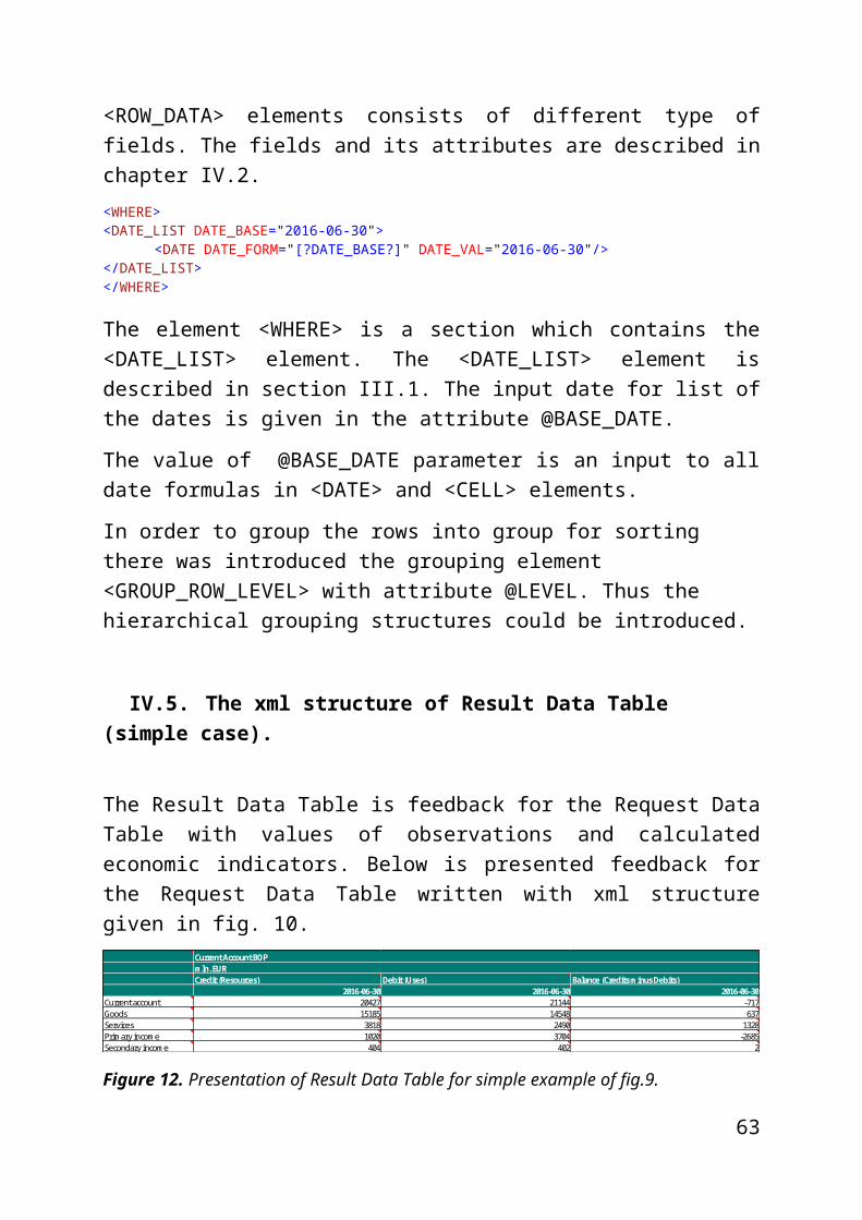
</FOR_ROWS> <WHERE> <DATE_LIST DATE_BASE="2016-06-30"> <DATE DATE_FORM="[?DATE_BASE?]-3*Y" /> <DATE DATE_FORM="[?DATE_BASE?]-2*Y" /> <DATE DATE_FORM="[?DATE_BASE?]-1*Y" /> <DATE DATE_FORM="[?DATE_BASE?]" /> </DATE_LIST> <LABEL_LIST DESC_ID="BOP_ITEM" CL_LIST="CL_ACCOUNTS_ITEM"> <LABEL DESC_ID="CA" DESC_VAL="Current Account" PL_DESC_VAL="Rachunek Bieżący" /> <LABEL DESC_ID="G" PL_DESC_VAL="Towary" /> <LABEL DESC_ID="S" PL_DESC_VAL="Usługi"/> <LABEL DESC_ID="IN1" PL_DESC_VAL="Dochody Pierwotne" /> <LABEL DESC_ID="IN2" PL_DESC_VAL="Dochody wtórne" /> </LABEL_LIST> <LABEL_LIST DESC_ID="BOP_ENTRY" CL_LIST="CL_ACCOUNT_ENTRY" > <LABEL DESC_ID="C" PL_DESC_VAL="Kredyt" /> <LABEL DESC_ID="D" PL_DESC_VAL="Debet" /> <LABEL DESC_ID="B" PL_DESC_VAL="Saldo"/> </LABEL_LIST> </WHERE> </SELECT>

Figure 25. The example 4 of simple Table Definition Query for Current Account of Polandfor 4 dates (spread over dates first and next spread over labels).

In example 4 the rows are grouped by dates and the group for one date consist of

several balance of payment items (components).

63


2013-06-30 Current account 50866 50641 225 Goods 35503 34979 524 Services 8309 6009 2300 Primary income 5440 8123 -2683 Secondary income 1613 1529 84

2014-06-30 Current account 53646 56161 -2515 Goods 39270 40107 -836 Services 9255 6689 2567 Primary income 3702 7811 -4108 Secondary income 1418 1555 -137




Figure 26. The example 4 of Result Data Table for Current Account of Poland

for 4 dates (spread over dates first and next spread over labels).

Let imagine we want to get similar table (to fig. 26) but with data for Germany.

Therefore in query instead of code “PL” for Poland should be put code “DE” for

Germany. The TDQ query for such case table is presented in example 5.

Example 5: <SELECT> <FOR_COLUMNS> <CAPTION DESC_VAL ="Current Account BOP" PL_DESC_VAL="Rachunek Bieżący"> <CAPTION DESC_VAL="mln. EUR" PL_DESC_VAL="mln. Eur"> <SPREAD_OVER_LABELS DIM_ID="COLS_1" TYPE="DEF_DESC" DESC_ID="BOP_ENTRY"> <CELL TS_TEMP="BP6.Q.N.DE.W1.S1.S1.T.[?COLS_1?].[?ROWS_1?]._Z._Z._Z.EUR._T._X.N" FORMULA="_C14"> <OBS_VAR OBS_ID="_C14" TS_TEMP="BP6.Q.N.DE.W1.S1.S1.T.[?COLS_1?].[?ROWS_1?]._Z._Z._Z.EUR._T._X.N" DATE_FORM="[?DATE_CELL?]" /> </CELL> </SPREAD_OVER_LABELS> </CAPTION> </CAPTION> </FOR_COLUMNS> <FOR_ROWS> <SPREAD_OVER_DATES > <SPREAD_OVER_LABELS DIM_ID="ROWS_1" TYPE="DEF_DESC" DESC_ID="BOP_ITEM">

64

</SPREAD_OVER_LABELS> </SPREAD_OVER_DATES></FOR_ROWS> <WHERE> <DATE_LIST DATE_BASE="2016-06-30"> <DATE DATE_FORM="[?DATE_BASE?]-3*Y" /> <DATE DATE_FORM="[?DATE_BASE?]-2*Y" /> <DATE DATE_FORM="[?DATE_BASE?]-1*Y" /> <DATE DATE_FORM="[?DATE_BASE?]" /> </DATE_LIST> <LABEL_LIST DESC_ID="BOP_ITEM" CL_LIST="CL_ACCOUNTS_ITEM"> <LABEL DESC_ID="CA" DESC_VAL="Current Account" PL_DESC_VAL="Rachunek Bieżący" /> <LABEL DESC_ID="G" PL_DESC_VAL="Towary" /> <LABEL DESC_ID="S" PL_DESC_VAL="Usługi"/> <LABEL DESC_ID="IN1" PL_DESC_VAL="Dochody Pierwotne" /> <LABEL DESC_ID="IN2" PL_DESC_VAL="Dochody wtórne" /> </LABEL_LIST> <LABEL_LIST DESC_ID="BOP_ENTRY" CL_LIST="CL_ACCOUNT_ENTRY" > <LABEL DESC_ID="C" PL_DESC_VAL="Kredyt" /> <LABEL DESC_ID="D" PL_DESC_VAL="Debet" /> <LABEL DESC_ID="B" PL_DESC_VAL="Saldo"/> </LABEL_LIST> </WHERE> </SELECT>Figure 27. The example 5 of simple Table Definition Query for Current Account of Germanyfor 4 dates (spread over dates first and next spread over labels).

The introduced changes of codes were marked by yellow color.


2013-06-30 Current account 383326 338305 45022 Goods 270749 215595 55153 Services 49980 60122 -10142 Primary income 47363 39933 7430 Secondary income 15235 22654 -7420





Figure 28. The example 5 of Result Data Table for Current Account of Germany

65

for 4 dates (spread over dates first and next spread over labels).

The values in table 28 are greater than in table 26 because economy of Germany

is greater than economy of Poland.

The next example is presentation of similar table but for two countries Germany

and Italy.

Example 6: <SELECT> <FOR_COLUMNS> <CAPTION DESC_VAL ="Current Account BOP" PL_DESC_VAL="Rachunek Bieżący"> <CAPTION DESC_VAL="mln. EUR" PL_DESC_VAL="mln. Eur"> <SPREAD_OVER_LABELS DIM_ID="COLS_1" TYPE="DEF_DESC" DESC_ID="BOP_ENTRY"> <CELL TS_TEMP="BP6.Q.N.[?ROWS_2?].W1.S1.S1.T.[?COLS_1?].[?ROWS_1?]._Z._Z._Z.EUR._T._X.N" FORMULA="_C14"> <OBS_VAR OBS_ID="_C14" TS_TEMP="BP6.Q.N.[?ROWS_2?].W1.S1.S1.T.[?COLS_1?].[?ROWS_1?]._Z._Z._Z.EUR._T._X.N" DATE_FORM="[?DATE_CELL?]" /> </CELL> </SPREAD_OVER_LABELS> </CAPTION> </CAPTION> </FOR_COLUMNS> <FOR_ROWS> <SPREAD_OVER_LABELS DIM_ID="ROWS_2" TYPE="DEF_DESC" DESC_ID="REGION"> <SPREAD_OVER_LABELS DIM_ID="ROWS_1" TYPE="DEF_DESC" DESC_ID="BOP_ITEM"> <SPREAD_OVER_DATES /> </SPREAD_OVER_LABELS> </SPREAD_OVER_LABELS></FOR_ROWS> <WHERE> <DATE_LIST DATE_BASE="2016-06-30"> <DATE DATE_FORM="[?DATE_BASE?]-3*Y" /> <DATE DATE_FORM="[?DATE_BASE?]-2*Y" /> <DATE DATE_FORM="[?DATE_BASE?]-1*Y" /> <DATE DATE_FORM="[?DATE_BASE?]" /> </DATE_LIST> <LABEL_LIST DESC_ID="BOP_ITEM" CL_LIST="CL_ACCOUNTS_ITEM"> <LABEL DESC_ID="CA" DESC_VAL="Current Account" PL_DESC_VAL="Rachunek Bieżący" /> <LABEL DESC_ID="G" PL_DESC_VAL="Towary" /> <LABEL DESC_ID="S" PL_DESC_VAL="Usługi"/> </LABEL_LIST> <LABEL_LIST DESC_ID="BOP_ENTRY" CL_LIST="CL_ACCOUNT_ENTRY" > <LABEL DESC_ID="C" PL_DESC_VAL="Kredyt" /> <LABEL DESC_ID="D" PL_DESC_VAL="Debet" /> <LABEL DESC_ID="B" PL_DESC_VAL="Saldo"/> </LABEL_LIST> <LABEL_LIST DESC_ID="REGION" CL_LIST="CL_AREA_EE"> <LABEL DESC_ID="DE" PL_DESC_VAL="Niemcy" /> <LABEL DESC_ID="IT" DESC_VAL="ITALY" PL_DESC_VAL="Włochy" /> </LABEL_LIST> </WHERE> </SELECT>

Figure 29. The example 6 Table Definition Query for Current Account of Germany and Italy quarterly frequency (spread over reference area, bop items and dates).

The table contain hierarchy of row descriptions starting from reference area labels, next with bop items and finally with sequence of dates.

66


Germany Current account 2013-06-30 383326 338305 45022 2014-06-30 394117 348158 45959 2015-06-30 425477 366121 59356 2016-06-30 434984 364978 70006 Goods 2013-06-30 270749 215595 55153 2014-06-30 274840 219956 54885 2015-06-30 297852 229193 68659 2016-06-30 306352 228488 77864 Services 2013-06-30 49980 60122 -10142 2014-06-30 54656 59466 -4811 2015-06-30 60096 62967 -2871 2016-06-30 62787 66862 -4075Italy Current account 2013-06-30 137235 132450 4785 2014-06-30 140438 134373 6065 2015-06-30 146192 142610 3581 2016-06-30 148061 136617 11444 Goods 2013-06-30 97117 86076 11041 2014-06-30 98735 87000 11735 2015-06-30 105147 93067 12079 2016-06-30 106101 89465 16636 Services 2013-06-30 22001 20867 1134 2014-06-30 22197 21380 818 2015-06-30 23301 22239 1062 2016-06-30 23405 23214 192


Figure 30. The example 6 Result Data Table for Current Account of Germany, Italy annual.

The example 7 presents transformation of data from quarter frequency to annual

frequency. The example contains the data for Current Account for Poland which

are aggregated from quarters to years.

Example 7: <SELECT> <FOR_COLUMNS> <CAPTION DESC_VAL ="Current Account BOP" PL_DESC_VAL="Rachunek Bieżący"> <CAPTION DESC_VAL="mln. EUR" PL_DESC_VAL="mln. Eur"> <SPREAD_OVER_LABELS DIM_ID="COLS_1" TYPE="DEF_DESC" DESC_ID="BOP_ENTRY"> <CELL TS_TEMP="BP6.A.N.PL.W1.S1.S1.T.[?COLS_1?].[?ROWS_1?]._Z._Z._Z.EUR._T._X.N" FORMULA="_C11+_C12+_C13+_C14">

<OBS_VAR OBS_ID="_C11" DATE_FORM="[?DATE_CELL?]-3*Q" TS_TEMP="BP6.Q.N.PL.W1.S1.S1.T.[?COLS_1?].[?ROWS_1?]._Z._Z._Z.EUR._T._X.N" /><OBS_VAR OBS_ID="_C12" DATE_FORM="[?DATE_CELL?]-2*Q" TS_TEMP="BP6.Q.N.PL.W1.S1.S1.T.[?COLS_1?].[?ROWS_1?]._Z._Z._Z.EUR._T._X.N" />

67

<OBS_VAR OBS_ID="_C13" DATE_FORM="[?DATE_CELL?]-1*Q" TS_TEMP="BP6.Q.N.PL.W1.S1.S1.T.[?COLS_1?].[?ROWS_1?]._Z._Z._Z.EUR._T._X.N" /><OBS_VAR OBS_ID="_C14" DATE_FORM="[?DATE_CELL?]" TS_TEMP="BP6.Q.N.PL.W1.S1.S1.T.[?COLS_1?].[?ROWS_1?]._Z._Z._Z.EUR._T._X.N" />

</CELL> </SPREAD_OVER_LABELS> </CAPTION> </CAPTION> </FOR_COLUMNS> <FOR_ROWS> <SPREAD_OVER_DATES > <SPREAD_OVER_LABELS DIM_ID="ROWS_1" TYPE="DEF_DESC" DESC_ID="BOP_ITEM"> </SPREAD_OVER_LABELS> </SPREAD_OVER_DATES> </FOR_ROWS> <WHERE> <DATE_LIST DATE_BASE="2016-12-31"> <DATE DATE_FORM="[?DATE_BASE?]-3*Y" /> <DATE DATE_FORM="[?DATE_BASE?]-2*Y" /> <DATE DATE_FORM="[?DATE_BASE?]-1*Y" /> <DATE DATE_FORM="[?DATE_BASE?]" /> </DATE_LIST> <LABEL_LIST DESC_ID="BOP_ITEM" CL_LIST="CL_ACCOUNTS_ITEM"> <LABEL DESC_ID="CA" DESC_VAL="Current Account" PL_DESC_VAL="Rachunek Bieżący" /> <LABEL DESC_ID="G" PL_DESC_VAL="Towary" /> <LABEL DESC_ID="S" PL_DESC_VAL="Usługi"/> <LABEL DESC_ID="IN1" PL_DESC_VAL="Dochody Pierwotne" /> <LABEL DESC_ID="IN2" PL_DESC_VAL="Dochody wtórne" /> </LABEL_LIST> <LABEL_LIST DESC_ID="BOP_ENTRY" CL_LIST="CL_ACCOUNT_ENTRY" > <LABEL DESC_ID="C" PL_DESC_VAL="Kredyt" /> <LABEL DESC_ID="D" PL_DESC_VAL="Debet" /> <LABEL DESC_ID="B" PL_DESC_VAL="Saldo"/> </LABEL_LIST> </WHERE> </SELECT>

Figure 31. The example 7 Table Definition Query for transformation from quarters to years for Current Account for Poland.

The cell should contain value of sum of four sequential quarters observations. In

such case (fig. 31) the <CELL> element contains 4 <OBS_VAR> elements

which are summarized into one year.

The <CELL> element contains attribute

@FORMULA=”_C11+_C12+_C13+_C14” which contains formula for sum of

4 observations pointed by attribute @OBS_ID. The value of cell @CELL_VAL

is calculated by substitution of observation values in the formula. Therefore the

cell value is calculated as sum of four observations.

68




2015-12-31 Current account 229087 231707 -2617 Goods 171643 169386 2256 Services 40502 29630 10872 Primary income 11166 26031 -14864 Secondary income 5776 6657 -881

2016-12-31 Current account 237964 238869 -905 Goods 176984 175063 1921 Services 44299 30595 13705 Primary income 11006 26463 -15456 Secondary income 5675 6748 -1073


Figure 32. The example 7 Result Data Table for transformation from quarters to years for Current Account for Poland.

The example 8 presents transformation of values of current account components for Poland from million Euro to percentage of GDP. Such data are well prepared for international comparison.

Example 8:<SELECT> <FOR_COLUMNS> <CAPTION DESC_VAL ="Current Account BOP" PL_DESC_VAL="Rachunek Bieżący"> <CAPTION DESC_VAL="% GDP" PL_DESC_VAL="% PKB"> <SPREAD_OVER_LABELS DIM_ID="COLS_1" TYPE="DEF_DESC" DESC_ID="BOP_ENTRY"> <CELL FORMULA="((_C11+_C12+_C13+_C14)/(_A11+_A12+_A13+_A14))*100" TS_TEMP="BP6.Q.N.PL.W1.S1.S1.T.[?COLS_1?].[?ROWS_1?]._Z._Z._Z.XDC_R_B1GQ_CY._T._X.N" >

<OBS_VAR OBS_ID="_C11" DATE_FORM="[?DATE_CELL?]-3*Q" TS_TEMP="BP6.Q.N.PL.W1.S1.S1.T.[?COLS_1?].[?ROWS_1?]._Z._Z._Z.EUR._T._X.N" /><OBS_VAR OBS_ID="_C12" DATE_FORM="[?DATE_CELL?]-2*Q" TS_TEMP="BP6.Q.N.PL.W1.S1.S1.T.[?COLS_1?].[?ROWS_1?]._Z._Z._Z.EUR._T._X.N" /><OBS_VAR OBS_ID="_C13" DATE_FORM="[?DATE_CELL?]-1*Q" TS_TEMP="BP6.Q.N.PL.W1.S1.S1.T.[?COLS_1?].[?ROWS_1?]._Z._Z._Z.EUR._T._X.N" /><OBS_VAR OBS_ID="_C14" DATE_FORM="[?DATE_CELL?]" TS_TEMP="BP6.Q.N.PL.W1.S1.S1.T.[?COLS_1?].[?ROWS_1?]._Z._Z._Z.EUR._T._X.N" /><OBS_VAR OBS_ID="_A11" TS_TEMP="MNA.Q.N.PL.W2.S1.S1.B.B1GQ._Z._Z._Z.EUR.V.N" DATE_FORM="[?DATE_CELL?]-3*Q" /><OBS_VAR OBS_ID="_A12" TS_TEMP="MNA.Q.N.PL.W2.S1.S1.B.B1GQ._Z._Z._Z.EUR.V.N" DATE_FORM="[?DATE_CELL?]-2*Q" />

69

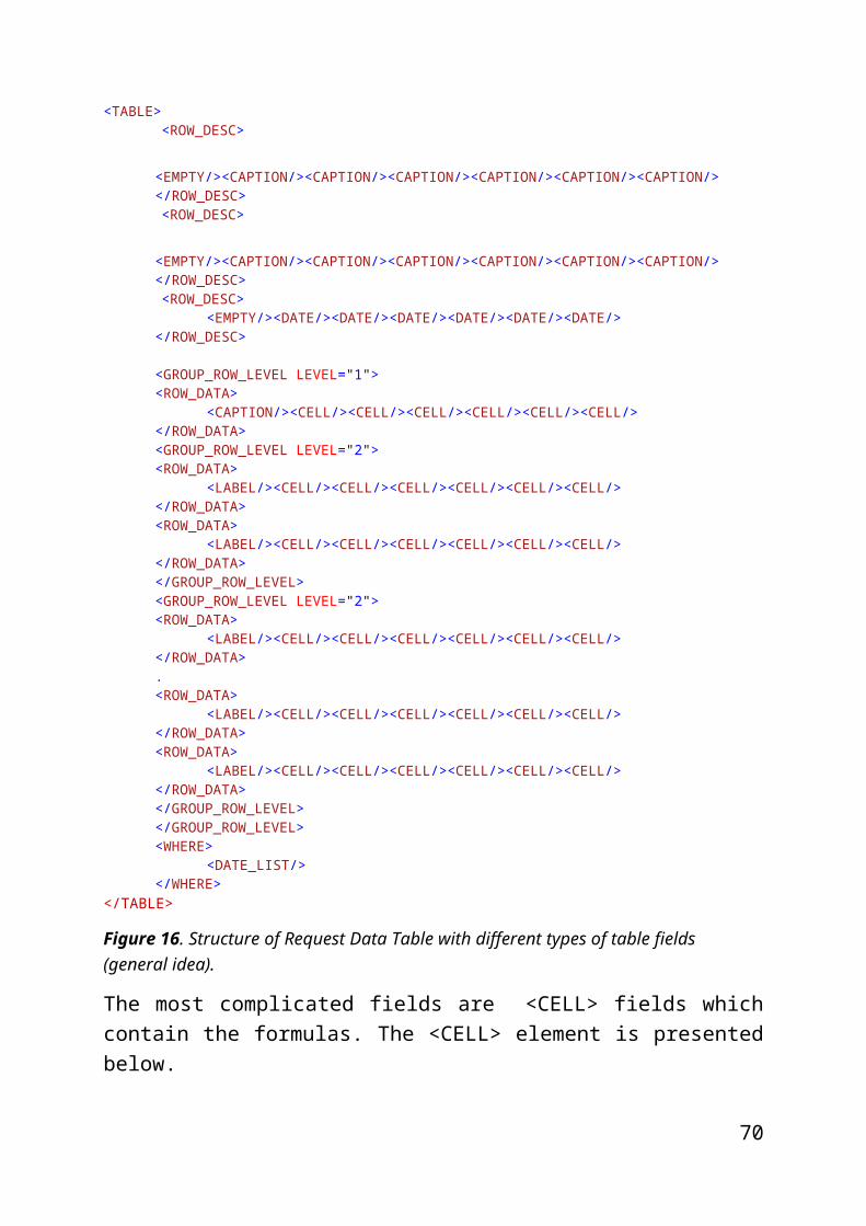
<OBS_VAR OBS_ID="_A13" TS_TEMP="MNA.Q.N.PL.W2.S1.S1.B.B1GQ._Z._Z._Z.EUR.V.N" DATE_FORM="[?DATE_CELL?]-1*Q" /><OBS_VAR OBS_ID="_A14" TS_TEMP="MNA.Q.N.PL.W2.S1.S1.B.B1GQ._Z._Z._Z.EUR.V.N" DATE_FORM="[?DATE_CELL?]" />

</CELL> </SPREAD_OVER_LABELS> </CAPTION> </CAPTION> </FOR_COLUMNS> <FOR_ROWS> <SPREAD_OVER_DATES > <SPREAD_OVER_LABELS DIM_ID="ROWS_1" TYPE="DEF_DESC" DESC_ID="BOP_ITEM"> </SPREAD_OVER_LABELS> </SPREAD_OVER_DATES> </FOR_ROWS> <WHERE> <DATE_LIST DATE_BASE="2016-12-31"> <DATE DATE_FORM="[?DATE_BASE?]-3*Y" /> <DATE DATE_FORM="[?DATE_BASE?]-2*Y" /> <DATE DATE_FORM="[?DATE_BASE?]-1*Y" /> <DATE DATE_FORM="[?DATE_BASE?]" /> </DATE_LIST> <LABEL_LIST DESC_ID="BOP_ITEM" CL_LIST="CL_ACCOUNTS_ITEM"> <LABEL DESC_ID="CA" DESC_VAL="Current Account" PL_DESC_VAL="Rachunek Bieżący" /> <LABEL DESC_ID="G" PL_DESC_VAL="Towary" /> <LABEL DESC_ID="S" PL_DESC_VAL="Usługi"/> <LABEL DESC_ID="IN1" PL_DESC_VAL="Dochody Pierwotne" /> <LABEL DESC_ID="IN2" PL_DESC_VAL="Dochody wtórne" /> </LABEL_LIST> <LABEL_LIST DESC_ID="BOP_ENTRY" CL_LIST="CL_ACCOUNT_ENTRY" > <LABEL DESC_ID="C" PL_DESC_VAL="Kredyt" /> <LABEL DESC_ID="D" PL_DESC_VAL="Debet" /> <LABEL DESC_ID="B" PL_DESC_VAL="Saldo"/> </LABEL_LIST> </WHERE> </SELECT>

Figure 33. The example 8 Table Definition Query for transformation for Current Account for Poland (yearly) from million Euro to percentage of GDP.

The formula for calculation of cell value is following: FORMULA="((_C11+_C12+_C13+_C14)/(_A11+_A12+_A13+_A14))*100"

where

_C11,_C12,_C13,_C14 are sequence of 4 vales quarter observations for balance of payment item,

_A11,_A12,_A13,_A14 are sequence of 4 vales quarter observations for gross domestic product,

In order to get the value in percent the ratio is multiplied by 100.

70


2013-12-31 Current account 50,4003 51,6781 -1,2781 Goods 37,5343 37,6217 -0,0874 Services 8,454 6,5346 1,9195 Primary income 2,8921 5,8962 -3,0044 Secondary income 1,5195 1,6254 -0,1056

2014-12-31 Current account 51,6861 53,7602 -2,0741 Goods 38,5084 39,2974 -0,7885 Services 8,9163 6,7159 2,2004 Primary income 2,8188 6,2119 -3,3929 Secondary income 1,4426 1,5353 -0,093

2015-12-31 Current account 53,288 53,8975 -0,6087 Goods 39,926 39,401 0,5248 Services 9,4212 6,8922 2,5289 Primary income 2,5973 6,0551 -3,4575 Secondary income 1,3436 1,5485 -0,2049

2016-12-31 Current account 56,0961 56,3094 -0,2133 Goods 41,721 41,2682 0,4528 Services 10,4428 7,2123 3,2307 Primary income 2,5945 6,2382 -3,6435 Secondary income 1,3378 1,5907 -0,2529

Current Account BOP% GDP

Figure 34. The example 8 Result Data Table for Current Account for Poland in percent of GDP.

The example 9 presents comparison of balance of current account as a percentage of GDP for different countries of Europe. The results are sorted in descending order for the data from last column.

Example 9: <SELECT> <FOR_COLUMNS> <CAPTION DESC_VAL ="Current Account BOP" PL_DESC_VAL="Rachunek Bieżący"> <CAPTION DESC_VAL="% GDP" PL_DESC_VAL="% PKB"> <SPREAD_OVER_DATES> <CELL TS_TEMP="BP6.Q.N.[?ROWS_1?].W1.S1.S1.T.B.CA._Z._Z._Z.XDC_R_B1GQ_CY._T._X.N"

FORMULA="((_C11+_C12+_C13+_C14)/(_A11+_A12+_A13+_A14))*100" SORT="DESC" COL_SORT="LAST">

<OBS_VAR OBS_ID="_C11" TS_TEMP="BP6.Q.N.[?ROWS_1?].W1.S1.S1.T.B.CA._Z._Z._Z.EUR._T._X.N" DATE_FORM="[?DATE_CELL?]-3*Q" /> <OBS_VAR OBS_ID="_C12" TS_TEMP="BP6.Q.N.[?ROWS_1?].W1.S1.S1.T.B.CA._Z._Z._Z.EUR._T._X.N" DATE_FORM="[?DATE_CELL?]-2*Q" /> <OBS_VAR OBS_ID="_C13" TS_TEMP="BP6.Q.N.[?ROWS_1?].W1.S1.S1.T.B.CA._Z._Z._Z.EUR._T._X.N" DATE_FORM="[?DATE_CELL?]-1*Q" /> <OBS_VAR OBS_ID="_C14" TS_TEMP="BP6.Q.N.[?ROWS_1?].W1.S1.S1.T.B.CA._Z._Z._Z.EUR._T._X.N" DATE_FORM="[?DATE_CELL?]" /> <OBS_VAR OBS_ID="_A11" TS_TEMP="MNA.Q.N.[?ROWS_1?].W2.S1.S1.B.B1GQ._Z._Z._Z.EUR.V.N" DATE_FORM="[?DATE_CELL?]-3*Q" />

71

<OBS_VAR OBS_ID="_A12" TS_TEMP="MNA.Q.N.[?ROWS_1?].W2.S1.S1.B.B1GQ._Z._Z._Z.EUR.V.N" DATE_FORM="[?DATE_CELL?]-2*Q" /> <OBS_VAR OBS_ID="_A13" TS_TEMP="MNA.Q.N.[?ROWS_1?].W2.S1.S1.B.B1GQ._Z._Z._Z.EUR.V.N" DATE_FORM="[?DATE_CELL?]-1*Q" /> <OBS_VAR OBS_ID="_A14" TS_TEMP="MNA.Q.N.[?ROWS_1?].W2.S1.S1.B.B1GQ._Z._Z._Z.EUR.V.N" DATE_FORM="[?DATE_CELL?]" /> </CELL> </SPREAD_OVER_DATES > </CAPTION> </CAPTION> </FOR_COLUMNS> <FOR_ROWS> <SPREAD_OVER_LABELS DIM_ID="ROWS_1" TYPE="DEF_DESC" DESC_ID="REGION"> </SPREAD_OVER_LABELS> </FOR_ROWS> <WHERE> -<DATE_LIST DATE_BASE="2015-12-31"> <DATE DATE_FORM="[?DATE_BASE?]-4*Y" DATE_VAL="2011-12-31"/> <DATE DATE_FORM="[?DATE_BASE?]-3*Y" DATE_VAL="2012-12-31"/> <DATE DATE_FORM="[?DATE_BASE?]-2*Y" DATE_VAL="2013-12-31"/> <DATE DATE_FORM="[?DATE_BASE?]-1*Y" DATE_VAL="2014-12-31"/> <DATE DATE_FORM="[?DATE_BASE?]" DATE_VAL="2015-12-31"/> <DATE DATE_FORM="[?DATE_BASE?]+1*Y" DATE_VAL="2016-12-31"/> </DATE_LIST> -<LABEL_LIST DESC_ID="REGION" CL_LIST="CL_AREA_EE"> -<CAPTION PL_DESC_VAL="Unia Monetarna" DESC_VAL="EUROPEAN MONETARY UNION" DESC_ID="EMU"> <LABEL PL_DESC_VAL="Niemcy" DESC_ID="DE"/> <LABEL PL_DESC_VAL="Francja" DESC_ID="FR"/> <LABEL PL_DESC_VAL="Włochy" DESC_VAL="ITALY" DESC_ID="IT"/> <LABEL PL_DESC_VAL="Hiszpania" DESC_VAL="SPAIN" DESC_ID="ES"/> <LABEL PL_DESC_VAL="Holandia" DESC_VAL="NETHERLAND" DESC_ID="NL"/> <LABEL PL_DESC_VAL="Belgia" DESC_VAL="BELGIUM" DESC_ID="BE"/> <LABEL PL_DESC_VAL="Austria" DESC_VAL="AUSTRIA" DESC_ID="AT"/> <LABEL PL_DESC_VAL="Finlandia" DESC_VAL="FINLAND" DESC_ID="FI"/> <LABEL PL_DESC_VAL="Irlandia" DESC_VAL="IRELAND" DESC_ID="IE"/> <LABEL PL_DESC_VAL="Grecja" DESC_VAL="GRECE" DESC_ID="GR"/> <LABEL PL_DESC_VAL="Portugalia" DESC_VAL="PORTUGAL" DESC_ID="PT"/> <LABEL PL_DESC_VAL="Słowacja" DESC_VAL="SLOVAKIA" DESC_ID="SK"/> <LABEL PL_DESC_VAL="Luksemburg" DESC_VAL="LUXEMBURG" DESC_ID="LU"/> <LABEL PL_DESC_VAL="Słowenia" DESC_VAL="SLOVENIA" DESC_ID="SI"/> <LABEL PL_DESC_VAL="Łotwa" DESC_VAL="LATVIA" DESC_ID="LV"/> <LABEL PL_DESC_VAL="Litwa" DESC_VAL="LITHUANIA" DESC_ID="LT"/> <LABEL PL_DESC_VAL="Cypr" DESC_VAL="CYPRUS" DESC_ID="CY"/>= <LABEL PL_DESC_VAL="Estonia" DESC_VAL="ESTONIA" DESC_ID="EE"/> <LABEL PL_DESC_VAL="Malta" DESC_VAL="MALTA" DESC_ID="MT"/> </CAPTION> -<CAPTION PL_DESC_VAL="Poza Unią Monetarną" DESC_VAL="NON EUROPEAN MONETARY UNION" DESC_ID="NON_EMU"> <LABEL PL_DESC_VAL="Polska" DESC_VAL="POLAND" DESC_ID="PL"/> <LABEL PL_DESC_VAL="Dania" DESC_VAL="DENMARK" DESC_ID="DK"/> <LABEL PL_DESC_VAL="Czechy" DESC_VAL="CZECH" DESC_ID="CZ"/> <LABEL PL_DESC_VAL="Szwecja" DESC_VAL="SWEDEN" DESC_ID="SE"/> <LABEL PL_DESC_VAL="Rumunia" DESC_VAL="ROMANIA" DESC_ID="RO"/> <LABEL PL_DESC_VAL="Węgry" DESC_VAL="HUNGARY" DESC_ID="HU"/> <LABEL PL_DESC_VAL="Bułgaria" DESC_VAL="BULGARY" DESC_ID="BG"/> <LABEL PL_DESC_VAL="Chorwacja" DESC_VAL="CROATIA" DESC_ID="HR"/> </CAPTION> </LABEL_LIST> </WHERE> </SELECT>

Figure 35. The example 8 Table Definition Query for Balance of Current Account as a percent of GDP for different countries of Europe sorted according to value from last column.

The example 9 presents the Balance of Current Account as a percentage of GDP for different European countries.

72

The results are sorted in descending order for values from last column. The instruction for sorting is placed in <CELL> element in attributes @COL_SORT=”LAST” and the order of sorting @SORT=”DESC”.

2011-12-31 2012-12-31 2013-12-31 2014-12-31 2015-12-31 2016-12-31EUROPEAN MONETARY UNION Netherlands 8,6965 10,3386 9,8664 8,8904 8,5934 8,4763 Germany 6,1069 7,0185 6,7092 7,4349 8,5412 8,3071 Malta -0,2049 1,691 2,6604 10,1618 5,1979 6,9931 Slovenia 0,1843 2,1554 4,438 5,8368 4,4024 5,2981 Luxembourg 6,0489 5,8759 5,5487 5,0229 5,1204 4,7139 Ireland -2,3654 -2,623 2,1381 1,6465 9,9822 4,5521 Italy -3,0108 -0,3609 0,9629 1,8808 1,4424 2,5608 Estonia 1,3379 -1,9515 -0,3547 0,9161 2,2023 2,0462 Spain -3,1801 -0,2312 1,5201 1,0844 1,3689 1,9281 Austria 1,6385 1,49 1,9514 2,3894 1,9085 1,7181 Latvia -3,1726 -3,5992 -2,7204 -1,9593 -0,7756 1,4747 Portugal -6,0017 -1,7922 1,5622 0,0607 0,0696 0,8414 Belgium -1,0728 -0,0542 -0,3183 -0,6742 0,4419 -0,3961 Greece -10,0049 -3,8305 -2,0398 -1,6387 0,1172 -0,6356 Slovakia -4,9513 0,9394 1,8592 1,1455 0,1652 -0,7288 France -0,9888 -1,2205 -0,8738 -1,2671 -0,4386 -0,8509 Lithuania -3,8625 -1,1785 1,5371 3,5993 -2,3359 -0,8852 Finland -1,7794 -1,934 -1,6028 -1,259 -0,5936 -1,0621 Cyprus -4,1103 -5,9691 -4,9452 -4,3261 -2,9143 -5,2622NON EUROPEAN MONETARY UNION Denmark 6,5887 6,2775 7,0356 8,905 9,1502 7,9356 Hungary 0,779 1,7702 3,7644 2,0446 3,2811 5,375 Sweden 5,5156 5,6201 5,2679 4,6016 4,7283 4,5091 Bulgaria 0,3318 -0,8535 1,2735 0,0818 -0,1347 4,1994 Croatia -0,8388 -0,1206 0,945 2,0613 4,9521 2,5397 Czech Republic -2,1024 -1,5463 -0,5283 0,1851 0,2249 1,1022 Poland -5,052 -3,7519 -1,2781 -2,0741 -0,6087 -0,2133 Romania -4,8889 -4,7988 -1,0657 -0,6738 -1,2221 -2,3235

Current Account BOP% GDP

Figure 36. The example 9 Result Data Table for Current Account as a percent of GDP for different countries of Europe sorted according to value from last column.

The results of query of example 9 is presented in fig. 29.

Example 10: <SELECT> <FOR_COLUMNS> <CAPTION DESC_VAL ="Net Inernational Investment Position" PL_DESC_VAL="Międzynarodowa Pozycja Inwestycyjna"> <CAPTION DESC_VAL="GDP %" PL_DESC_VAL="PKB %"> <SPREAD_OVER_DATES > <CELL TS_TEMP="BP6.Q.N.[?ROWS1_ID?].W1.S1.S1.LE.N.FA._Z._Z._Z.XDC_R_B1GQ_CY._T._X.N" COL_SORT="LAST" SORT="DESC" FORMULA="(_C14/(_A11+_A12+_A13+_A14))*100" CONDITION="(CELL_VAL.GT.(-35.0))"> <OBS_VAR OBS_ID="_A11" TS_TEMP="MNA.Q.N.[?ROWS1_ID?].W2.S1.S1.B.B1GQ._Z._Z._Z.EUR.V.N" DATE_FORM="[?DATE_CELL?]-3*Q" /> <OBS_VAR OBS_ID="_A12" TS_TEMP="MNA.Q.N.[?ROWS1_ID?].W2.S1.S1.B.B1GQ._Z._Z._Z.EUR.V.N" DATE_FORM="[?DATE_CELL?]-2*Q" /> <OBS_VAR OBS_ID="_A13" TS_TEMP="MNA.Q.N.[?ROWS1_ID?].W2.S1.S1.B.B1GQ._Z._Z._Z.EUR.V.N" DATE_FORM="[?DATE_CELL?]-1*Q" /> <OBS_VAR OBS_ID="_A14" TS_TEMP="MNA.Q.N.[?ROWS1_ID?].W2.S1.S1.B.B1GQ._Z._Z._Z.EUR.V.N" DATE_FORM="[?DATE_CELL?]" /> <OBS_VAR OBS_ID="_C14" TS_TEMP="BP6.Q.N.[?ROWS1_ID?].W1.S1.S1.LE.N.FA._T.F._Z.EUR._T._X.N" DATE_FORM="[?DATE_CELL?]" /> </CELL> </SPREAD_OVER_DATES> </CAPTION> </CAPTION> </FOR_COLUMNS> <FOR_ROWS> <SPREAD_OVER_LABELS DIM_ID="ROWS1_ID" TYPE="DEF_DESC" DESC_ID="REGION"> </SPREAD_OVER_LABELS></FOR_ROWS>

73

<WHERE> <DATE_LIST DATE_BASE="2015-12-31"> <DATE DATE_FORM="[?DATE_BASE?]-4*Y" DATE_VAL="2011-12-31"/> <DATE DATE_FORM="[?DATE_BASE?]-3*Y" DATE_VAL="2012-12-31"/> <DATE DATE_FORM="[?DATE_BASE?]-2*Y" DATE_VAL="2013-12-31"/> <DATE DATE_FORM="[?DATE_BASE?]-1*Y" DATE_VAL="2014-12-31"/> <DATE DATE_FORM="[?DATE_BASE?]" DATE_VAL="2015-12-31"/> <DATE DATE_FORM="[?DATE_BASE?]+1*Y" DATE_VAL="2016-12-31"/> </DATE_LIST> <LABEL_LIST DESC_ID="REGION" CL_LIST="CL_AREA_EE"> <CAPTION DESC_ID="EMU" DESC_VAL="EUROPEAN MONETARY UNION" PL_DESC_VAL="Unia Monetarna"> <LABEL DESC_ID="DE" PL_DESC_VAL="Niemcy" /> <LABEL DESC_ID="FR" PL_DESC_VAL="Francja"/> <LABEL DESC_ID="IT" DESC_VAL="ITALY" PL_DESC_VAL="Włochy" /> <LABEL DESC_ID="ES" DESC_VAL="SPAIN" PL_DESC_VAL="Hiszpania" /> <LABEL DESC_ID="NL" DESC_VAL="NETHERLAND" PL_DESC_VAL="Holandia" /> <LABEL DESC_ID="BE" DESC_VAL="BELGIUM" PL_DESC_VAL="Belgia" /> <LABEL DESC_ID="AT" DESC_VAL="AUSTRIA" PL_DESC_VAL="Austria" /> <LABEL DESC_ID="FI" DESC_VAL="FINLAND" PL_DESC_VAL="Finlandia" /> <LABEL DESC_ID="IE" DESC_VAL="IRELAND" PL_DESC_VAL="Irlandia" /> <LABEL DESC_ID="GR" DESC_VAL="GRECE" PL_DESC_VAL="Grecja" /> <LABEL DESC_ID="PT" DESC_VAL="PORTUGAL" PL_DESC_VAL="Portugalia" /> <LABEL DESC_ID="SK" DESC_VAL="SLOVAKIA" PL_DESC_VAL="Słowacja"/> <LABEL DESC_ID="LU" DESC_VAL="LUXEMBURG" PL_DESC_VAL="Luksemburg" /> <LABEL DESC_ID="SI" DESC_VAL="SLOVENIA" PL_DESC_VAL="Słowenia"/> <LABEL DESC_ID="LV" DESC_VAL="LATVIA" PL_DESC_VAL="Łotwa"/> <LABEL DESC_ID="LT" DESC_VAL="LITHUANIA" PL_DESC_VAL="Litwa"/> <LABEL DESC_ID="CY" DESC_VAL="CYPRUS" PL_DESC_VAL="Cypr"/> <LABEL DESC_ID="EE" DESC_VAL="ESTONIA" PL_DESC_VAL="Estonia"/> <LABEL DESC_ID="MT" DESC_VAL="MALTA" PL_DESC_VAL="Malta"/> </CAPTION> <CAPTION DESC_ID="NON_EMU" DESC_VAL="NON EUROPEAN MONETARY UNION" PL_DESC_VAL="Poza Unią Monetarną"> <LABEL DESC_ID="PL" DESC_VAL="POLAND" PL_DESC_VAL="Polska"/> <LABEL DESC_ID="DK" DESC_VAL="DENMARK" PL_DESC_VAL="Dania"/> <LABEL DESC_ID="CZ" DESC_VAL="CZECH" PL_DESC_VAL="Czechy"/> <LABEL DESC_ID="SE" DESC_VAL="SWEDEN" PL_DESC_VAL="Szwecja" /> <LABEL DESC_ID="RO" DESC_VAL="ROMANIA" PL_DESC_VAL="Rumunia"/> <LABEL DESC_ID="HU" DESC_VAL="HUNGARY" PL_DESC_VAL="Węgry"/> <LABEL DESC_ID="BG" DESC_VAL="BULGARY" PL_DESC_VAL="Bułgaria"/> <LABEL DESC_ID="HR" DESC_VAL="CROATIA" PL_DESC_VAL="Chorwacja"/> </CAPTION> </LABEL_LIST> </WHERE> </SELECT>Figure 37. The example 10 Table Definition Query for Net Investment Position as a percent of GDP for different countries of Europe sorted according to value from last column in descending order. The example contains validation rule which is True when value is larger than -35%.

The example 10 presents the Net Investment Position as a percentage of GDP for different European countries.

The results are sorted in descending order for values from last column. The instruction for sorting is placed in <CELL> element in attributes @COL_SORT=”LAST” and the order of sorting @SORT=”DESC”.

The validation rule is saved in attribute @CONDITION=”(CELL_VAL.GT.(-35.0))”.

74

2011-12-31 2012-12-31 2013-12-31 2014-12-31 2015-12-31 2016-12-31EUROPEAN MONETARY UNION Netherlands 20,3585 27,0145 31,0337 57,8474 56,0546 68,7019 Germany 23,2232 28,3977 34,3492 40,752 49,5559 54,9431 Belgium 60,8983 51,7559 52,0255 59,3225 61,1774 49,5007 Malta 6,2652 19,6346 26,997 44,5673 52,0873 47,5569 Luxembourg 28,9056 51,9835 44,1964 33,0193 35,0442 23,2191 Austria -1,9233 -3,202 1,2988 2,2429 2,8953 7,4168 Finland 15,0984 11,7151 3,8527 -3,18 0,5401 7,0983 Italy -19,1696 -23,8568 -25,3182 -24,445 -23,5285 -14,9928 France -8,6639 -12,8305 -16,5695 -15,6313 -15,6753 -15,7476 Estonia -54,7589 -51,1296 -50,1162 -46,7196 -40,9003 -37,4296 Slovenia -45,1942 -50,1632 -47,5735 -46,1235 -40,0337 -37,4663 Lithuania -52,5366 -53,3581 -46,9715 -45,8376 -44,7221 -43,2896 Slovakia -64,4398 -61,4427 -62,3056 -63,7108 -60,4787 -57,5866 Latvia -74,4201 -67,2424 -66,3935 -64,1907 -62,4542 -58,1663 Spain -91,9404 -89,88 -94,3494 -97,4817 -91,3022 -85,7202 Portugal -100,7263 -116,5293 -116,341 -117,7011 -112,0463 -105,0961 Cyprus -129,8832 -129,2245 -138,9022 -147,3451 -130,3234 -125,4266 Greece -88,8097 -115,8802 -130,4182 -132,4791 -134,6018 -136,0867 Ireland -139,1724 -137,4291 -131,6008 -160,9996 -203,0584 -178,7242NON EUROPEAN MONETARY UNION Denmark 27,8122 36,0244 37,2371 44,1762 34,0033 55,9317 Sweden -8,0636 -14,8236 -12,2517 1,1192 3,376 15,6996 Czech Republic -43,1004 -45,9154 -39,195 -36,3033 -33,2118 -24,6401 Romania -64,2191 -67,7973 -61,9048 -56,7878 -53,8492 -48,8862 Bulgaria -82,7617 -77,886 -73,3204 -75,1949 -63,4891 -51,3216 Poland -57,7547 -67,0688 -69,6453 -67,6668 -61,2698 -61,0123 Hungary -94,4056 -92,9054 -83,4211 -75,4848 -63,1742 -61,4211 Croatia -90,5238 -90,3007 -88,3707 -86,49 -77,058 -70,5657


Figure 38. The example 10 Result Data Table for Net Investment Position as a percent of GDP for different countries of Europe sorted according to value from last column in descending order. The example contains validation rule which is True when value is larger than -35%.

The values which do not fulfill the condition are marked with yellow color.

The next example is very similar to 10 but the instruction for sorting order is in opposite direction in ascending order.

Example 11: <SELECT> <FOR_COLUMNS> <CAPTION DESC_VAL ="Net Inernational Investment Position" PL_DESC_VAL="Międzynarodowa Pozycja Inwestycyjna"> <CAPTION DESC_VAL="GDP %" PL_DESC_VAL="PKB %"> <SPREAD_OVER_DATES > <CELL TS_TEMP="BP6.Q.N.[?ROWS1_ID?].W1.S1.S1.LE.N.FA._Z._Z._Z.XDC_R_B1GQ_CY._T._X.N" COL_SORT="LAST" SORT="ASC" FORMULA="(_C14/(_A11+_A12+_A13+_A14))*100" CONDITION="(CELL_VAL.GT.(-35.0))"> <OBS_VAR OBS_ID="_A11" TS_TEMP="MNA.Q.N.[?ROWS1_ID?].W2.S1.S1.B.B1GQ._Z._Z._Z.EUR.V.N" DATE_FORM="[?DATE_CELL?]-3*Q" /> <OBS_VAR OBS_ID="_A12" TS_TEMP="MNA.Q.N.[?ROWS1_ID?].W2.S1.S1.B.B1GQ._Z._Z._Z.EUR.V.N" DATE_FORM="[?DATE_CELL?]-2*Q" /> <OBS_VAR OBS_ID="_A13" TS_TEMP="MNA.Q.N.[?ROWS1_ID?].W2.S1.S1.B.B1GQ._Z._Z._Z.EUR.V.N" DATE_FORM="[?DATE_CELL?]-1*Q" /> <OBS_VAR OBS_ID="_A14" TS_TEMP="MNA.Q.N.[?ROWS1_ID?].W2.S1.S1.B.B1GQ._Z._Z._Z.EUR.V.N" DATE_FORM="[?DATE_CELL?]" /> <OBS_VAR OBS_ID="_C14" TS_TEMP="BP6.Q.N.[?ROWS1_ID?].W1.S1.S1.LE.N.FA._T.F._Z.EUR._T._X.N" DATE_FORM="[?DATE_CELL?]" /> </CELL> </SPREAD_OVER_DATES> </CAPTION> </CAPTION> </FOR_COLUMNS> <FOR_ROWS> <SPREAD_OVER_LABELS DIM_ID="ROWS1_ID" TYPE="DEF_DESC" DESC_ID="REGION"> </SPREAD_OVER_LABELS></FOR_ROWS> <WHERE>

75

<DATE_LIST DATE_BASE="2015-12-31"> <DATE DATE_FORM="[?DATE_BASE?]-4*Y" DATE_VAL="2011-12-31"/> <DATE DATE_FORM="[?DATE_BASE?]-3*Y" DATE_VAL="2012-12-31"/> <DATE DATE_FORM="[?DATE_BASE?]-2*Y" DATE_VAL="2013-12-31"/> <DATE DATE_FORM="[?DATE_BASE?]-1*Y" DATE_VAL="2014-12-31"/> <DATE DATE_FORM="[?DATE_BASE?]" DATE_VAL="2015-12-31"/> <DATE DATE_FORM="[?DATE_BASE?]+1*Y" DATE_VAL="2016-12-31"/> </DATE_LIST> <LABEL_LIST DESC_ID="REGION" CL_LIST="CL_AREA_EE"> <CAPTION DESC_ID="EMU" DESC_VAL="EUROPEAN MONETARY UNION" PL_DESC_VAL="Unia Monetarna"> <LABEL DESC_ID="DE" PL_DESC_VAL="Niemcy" /> <LABEL DESC_ID="FR" PL_DESC_VAL="Francja"/> <LABEL DESC_ID="IT" DESC_VAL="ITALY" PL_DESC_VAL="Włochy" /> <LABEL DESC_ID="ES" DESC_VAL="SPAIN" PL_DESC_VAL="Hiszpania" /> <LABEL DESC_ID="NL" DESC_VAL="NETHERLAND" PL_DESC_VAL="Holandia" /> <LABEL DESC_ID="BE" DESC_VAL="BELGIUM" PL_DESC_VAL="Belgia" /> <LABEL DESC_ID="AT" DESC_VAL="AUSTRIA" PL_DESC_VAL="Austria" /> <LABEL DESC_ID="FI" DESC_VAL="FINLAND" PL_DESC_VAL="Finlandia" /> <LABEL DESC_ID="IE" DESC_VAL="IRELAND" PL_DESC_VAL="Irlandia" /> <LABEL DESC_ID="GR" DESC_VAL="GRECE" PL_DESC_VAL="Grecja" /> <LABEL DESC_ID="PT" DESC_VAL="PORTUGAL" PL_DESC_VAL="Portugalia" /> <LABEL DESC_ID="SK" DESC_VAL="SLOVAKIA" PL_DESC_VAL="Słowacja"/> <LABEL DESC_ID="LU" DESC_VAL="LUXEMBURG" PL_DESC_VAL="Luksemburg" /> <LABEL DESC_ID="SI" DESC_VAL="SLOVENIA" PL_DESC_VAL="Słowenia"/> <LABEL DESC_ID="LV" DESC_VAL="LATVIA" PL_DESC_VAL="Łotwa"/> <LABEL DESC_ID="LT" DESC_VAL="LITHUANIA" PL_DESC_VAL="Litwa"/> <LABEL DESC_ID="CY" DESC_VAL="CYPRUS" PL_DESC_VAL="Cypr"/> <LABEL DESC_ID="EE" DESC_VAL="ESTONIA" PL_DESC_VAL="Estonia"/> <LABEL DESC_ID="MT" DESC_VAL="MALTA" PL_DESC_VAL="Malta"/> </CAPTION> <CAPTION DESC_ID="NON_EMU" DESC_VAL="NON EUROPEAN MONETARY UNION" PL_DESC_VAL="Poza Unią Monetarną"> <LABEL DESC_ID="PL" DESC_VAL="POLAND" PL_DESC_VAL="Polska"/> <LABEL DESC_ID="DK" DESC_VAL="DENMARK" PL_DESC_VAL="Dania"/> <LABEL DESC_ID="CZ" DESC_VAL="CZECH" PL_DESC_VAL="Czechy"/> <LABEL DESC_ID="SE" DESC_VAL="SWEDEN" PL_DESC_VAL="Szwecja" /> <LABEL DESC_ID="RO" DESC_VAL="ROMANIA" PL_DESC_VAL="Rumunia"/> <LABEL DESC_ID="HU" DESC_VAL="HUNGARY" PL_DESC_VAL="Węgry"/> <LABEL DESC_ID="BG" DESC_VAL="BULGARY" PL_DESC_VAL="Bułgaria"/> <LABEL DESC_ID="HR" DESC_VAL="CROATIA" PL_DESC_VAL="Chorwacja"/> </CAPTION> </LABEL_LIST> </WHERE> </SELECT>Figure 39. The example 11 Table Definition Query for Net Investment Position as a percent of GDP for different countries of Europe sorted according to value from last column in ascending order. The example contains validation rule which is True when value is larger than -35%.

76

2011-12-31 2012-12-31 2013-12-31 2014-12-31 2015-12-31 2016-12-31EUROPEAN MONETARY UNION Ireland -139,1724 -137,4291 -131,6008 -160,9996 -203,0584 -178,7242 Greece -88,8097 -115,8802 -130,4182 -132,4791 -134,6018 -136,0867 Cyprus -129,8832 -129,2245 -138,9022 -147,3451 -130,3234 -125,4266 Portugal -100,7263 -116,5293 -116,341 -117,7011 -112,0463 -105,0961 Spain -91,9404 -89,88 -94,3494 -97,4817 -91,3022 -85,7202 Latvia -74,4201 -67,2424 -66,3935 -64,1907 -62,4542 -58,1663 Slovakia -64,4398 -61,4427 -62,3056 -63,7108 -60,4787 -57,5866 Lithuania -52,5366 -53,3581 -46,9715 -45,8376 -44,7221 -43,2896 Slovenia -45,1942 -50,1632 -47,5735 -46,1235 -40,0337 -37,4663 Estonia -54,7589 -51,1296 -50,1162 -46,7196 -40,9003 -37,4296 France -8,6639 -12,8305 -16,5695 -15,6313 -15,6753 -15,7476 Italy -19,1696 -23,8568 -25,3182 -24,445 -23,5285 -14,9928 Finland 15,0984 11,7151 3,8527 -3,18 0,5401 7,0983 Austria -1,9233 -3,202 1,2988 2,2429 2,8953 7,4168 Luxembourg 28,9056 51,9835 44,1964 33,0193 35,0442 23,2191 Malta 6,2652 19,6346 26,997 44,5673 52,0873 47,5569 Belgium 60,8983 51,7559 52,0255 59,3225 61,1774 49,5007 Germany 23,2232 28,3977 34,3492 40,752 49,5559 54,9431 Netherlands 20,3585 27,0145 31,0337 57,8474 56,0546 68,7019NON EUROPEAN MONETARY UNION Croatia -90,5238 -90,3007 -88,3707 -86,49 -77,058 -70,5657 Hungary -94,4056 -92,9054 -83,4211 -75,4848 -63,1742 -61,4211 Poland -57,7547 -67,0688 -69,6453 -67,6668 -61,2698 -61,0123 Bulgaria -82,7617 -77,886 -73,3204 -75,1949 -63,4891 -51,3216 Romania -64,2191 -67,7973 -61,9048 -56,7878 -53,8492 -48,8862 Czech Republic -43,1004 -45,9154 -39,195 -36,3033 -33,2118 -24,6401 Sweden -8,0636 -14,8236 -12,2517 1,1192 3,376 15,6996 Denmark 27,8122 36,0244 37,2371 44,1762 34,0033 55,9317


Figure 40. The example 11 Result Data Table for Net Investment Position as a percent of GDP for different countries of Europe sorted according to value from last column in ascending order. The example contains validation rule which is True when value is larger than -35%.

The values which do not fulfill the condition are marked with yellow color.

Another example 12 is for sorting according to the values from first column.<SELECT> <FOR_COLUMNS> <CAPTION DESC_VAL ="Net Inernational Investment Position" PL_DESC_VAL="Międzynarodowa Pozycja Inwestycyjna"> <CAPTION DESC_VAL="GDP %" PL_DESC_VAL="PKB %"> <SPREAD_OVER_DATES > <CELL TS_TEMP="BP6.Q.N.[?ROWS1_ID?].W1.S1.S1.LE.N.FA._Z._Z._Z.XDC_R_B1GQ_CY._T._X.N" COL_SORT="FIRST" SORT="DESC" FORMULA="(_C14/(_A11+_A12+_A13+_A14))*100" CONDITION="(CELL_VAL.GT.(-35.0))"> <OBS_VAR OBS_ID="_A11" TS_TEMP="MNA.Q.N.[?ROWS1_ID?].W2.S1.S1.B.B1GQ._Z._Z._Z.EUR.V.N" DATE_FORM="[?DATE_CELL?]-3*Q" /> <OBS_VAR OBS_ID="_A12" TS_TEMP="MNA.Q.N.[?ROWS1_ID?].W2.S1.S1.B.B1GQ._Z._Z._Z.EUR.V.N" DATE_FORM="[?DATE_CELL?]-2*Q" /> <OBS_VAR OBS_ID="_A13" TS_TEMP="MNA.Q.N.[?ROWS1_ID?].W2.S1.S1.B.B1GQ._Z._Z._Z.EUR.V.N" DATE_FORM="[?DATE_CELL?]-1*Q" /> <OBS_VAR OBS_ID="_A14" TS_TEMP="MNA.Q.N.[?ROWS1_ID?].W2.S1.S1.B.B1GQ._Z._Z._Z.EUR.V.N" DATE_FORM="[?DATE_CELL?]" /> <OBS_VAR OBS_ID="_C14" TS_TEMP="BP6.Q.N.[?ROWS1_ID?].W1.S1.S1.LE.N.FA._T.F._Z.EUR._T._X.N" DATE_FORM="[?DATE_CELL?]" /> </CELL> </SPREAD_OVER_DATES> </CAPTION> </CAPTION> </FOR_COLUMNS> <FOR_ROWS> <SPREAD_OVER_LABELS DIM_ID="ROWS1_ID" TYPE="DEF_DESC" DESC_ID="REGION"> </SPREAD_OVER_LABELS></FOR_ROWS> <WHERE> <DATE_LIST DATE_BASE="2015-12-31"> <DATE DATE_FORM="[?DATE_BASE?]-4*Y" DATE_VAL="2011-12-31"/> <DATE DATE_FORM="[?DATE_BASE?]-3*Y" DATE_VAL="2012-12-31"/> <DATE DATE_FORM="[?DATE_BASE?]-2*Y" DATE_VAL="2013-12-31"/>

77

<DATE DATE_FORM="[?DATE_BASE?]-1*Y" DATE_VAL="2014-12-31"/> <DATE DATE_FORM="[?DATE_BASE?]" DATE_VAL="2015-12-31"/> <DATE DATE_FORM="[?DATE_BASE?]+1*Y" DATE_VAL="2016-12-31"/> </DATE_LIST> <LABEL_LIST DESC_ID="REGION" CL_LIST="CL_AREA_EE"> <CAPTION DESC_ID="EMU" DESC_VAL="EUROPEAN MONETARY UNION" PL_DESC_VAL="Unia Monetarna"> <LABEL DESC_ID="DE" PL_DESC_VAL="Niemcy" /> <LABEL DESC_ID="FR" PL_DESC_VAL="Francja"/> <LABEL DESC_ID="IT" DESC_VAL="ITALY" PL_DESC_VAL="Włochy" /> <LABEL DESC_ID="ES" DESC_VAL="SPAIN" PL_DESC_VAL="Hiszpania" /> <LABEL DESC_ID="NL" DESC_VAL="NETHERLAND" PL_DESC_VAL="Holandia" /> <LABEL DESC_ID="BE" DESC_VAL="BELGIUM" PL_DESC_VAL="Belgia" /> <LABEL DESC_ID="AT" DESC_VAL="AUSTRIA" PL_DESC_VAL="Austria" /> <LABEL DESC_ID="FI" DESC_VAL="FINLAND" PL_DESC_VAL="Finlandia" /> <LABEL DESC_ID="IE" DESC_VAL="IRELAND" PL_DESC_VAL="Irlandia" /> <LABEL DESC_ID="GR" DESC_VAL="GRECE" PL_DESC_VAL="Grecja" /> <LABEL DESC_ID="PT" DESC_VAL="PORTUGAL" PL_DESC_VAL="Portugalia" /> <LABEL DESC_ID="SK" DESC_VAL="SLOVAKIA" PL_DESC_VAL="Słowacja"/> <LABEL DESC_ID="LU" DESC_VAL="LUXEMBURG" PL_DESC_VAL="Luksemburg" /> <LABEL DESC_ID="SI" DESC_VAL="SLOVENIA" PL_DESC_VAL="Słowenia"/> <LABEL DESC_ID="LV" DESC_VAL="LATVIA" PL_DESC_VAL="Łotwa"/> <LABEL DESC_ID="LT" DESC_VAL="LITHUANIA" PL_DESC_VAL="Litwa"/> <LABEL DESC_ID="CY" DESC_VAL="CYPRUS" PL_DESC_VAL="Cypr"/> <LABEL DESC_ID="EE" DESC_VAL="ESTONIA" PL_DESC_VAL="Estonia"/> <LABEL DESC_ID="MT" DESC_VAL="MALTA" PL_DESC_VAL="Malta"/> </CAPTION> <CAPTION DESC_ID="NON_EMU" DESC_VAL="NON EUROPEAN MONETARY UNION" PL_DESC_VAL="Poza Unią Monetarną"> <LABEL DESC_ID="PL" DESC_VAL="POLAND" PL_DESC_VAL="Polska"/> <LABEL DESC_ID="DK" DESC_VAL="DENMARK" PL_DESC_VAL="Dania"/> <LABEL DESC_ID="CZ" DESC_VAL="CZECH" PL_DESC_VAL="Czechy"/> <LABEL DESC_ID="SE" DESC_VAL="SWEDEN" PL_DESC_VAL="Szwecja" /> <LABEL DESC_ID="RO" DESC_VAL="ROMANIA" PL_DESC_VAL="Rumunia"/> <LABEL DESC_ID="HU" DESC_VAL="HUNGARY" PL_DESC_VAL="Węgry"/> <LABEL DESC_ID="BG" DESC_VAL="BULGARY" PL_DESC_VAL="Bułgaria"/> <LABEL DESC_ID="HR" DESC_VAL="CROATIA" PL_DESC_VAL="Chorwacja"/> </CAPTION> </LABEL_LIST> </WHERE> </SELECT>

Figure 41. The example 11 Table Definition Query for Net Investment Position as a percent of GDP for different countries of Europe sorted according to value from first column in descending order. The example contains validation rule which is True when value is larger than -35%.

78

2011-12-31 2012-12-31 2013-12-31 2014-12-31 2015-12-31 2016-12-31EUROPEAN MONETARY UNION Belgium 60,8983 51,7559 52,0255 59,3225 61,1774 49,5007 Luxembourg 28,9056 51,9835 44,1964 33,0193 35,0442 23,2191 Germany 23,2232 28,3977 34,3492 40,752 49,5559 54,9431 Netherlands 20,3585 27,0145 31,0337 57,8474 56,0546 68,7019 Finland 15,0984 11,7151 3,8527 -3,18 0,5401 7,0983 Malta 6,2652 19,6346 26,997 44,5673 52,0873 47,5569 Austria -1,9233 -3,202 1,2988 2,2429 2,8953 7,4168 France -8,6639 -12,8305 -16,5695 -15,6313 -15,6753 -15,7476 Italy -19,1696 -23,8568 -25,3182 -24,445 -23,5285 -14,9928 Slovenia -45,1942 -50,1632 -47,5735 -46,1235 -40,0337 -37,4663 Lithuania -52,5366 -53,3581 -46,9715 -45,8376 -44,7221 -43,2896 Estonia -54,7589 -51,1296 -50,1162 -46,7196 -40,9003 -37,4296 Slovakia -64,4398 -61,4427 -62,3056 -63,7108 -60,4787 -57,5866 Latvia -74,4201 -67,2424 -66,3935 -64,1907 -62,4542 -58,1663 Greece -88,8097 -115,8802 -130,4182 -132,4791 -134,6018 -136,0867 Spain -91,9404 -89,88 -94,3494 -97,4817 -91,3022 -85,7202 Portugal -100,7263 -116,5293 -116,341 -117,7011 -112,0463 -105,0961 Cyprus -129,8832 -129,2245 -138,9022 -147,3451 -130,3234 -125,4266 Ireland -139,1724 -137,4291 -131,6008 -160,9996 -203,0584 -178,7242NON EUROPEAN MONETARY UNION Denmark 27,8122 36,0244 37,2371 44,1762 34,0033 55,9317 Sweden -8,0636 -14,8236 -12,2517 1,1192 3,376 15,6996 Czech Republic -43,1004 -45,9154 -39,195 -36,3033 -33,2118 -24,6401 Poland -57,7547 -67,0688 -69,6453 -67,6668 -61,2698 -61,0123 Romania -64,2191 -67,7973 -61,9048 -56,7878 -53,8492 -48,8862 Bulgaria -82,7617 -77,886 -73,3204 -75,1949 -63,4891 -51,3216 Croatia -90,5238 -90,3007 -88,3707 -86,49 -77,058 -70,5657 Hungary -94,4056 -92,9054 -83,4211 -75,4848 -63,1742 -61,4211


Figure 42. The example 12 Result Data Table for Net Investment Position as a percent of GDP for different countries of Europe sorted according to value from first column in descending order. The example contains validation rule which is True when value is larger than -35%.

The Result Data Tables are available in 3 formats:

Excel format,

PDF format,

Xml-format which can be ease transform using xsl style sheets to HTML.

Thus the technique of Table Definition Queries is an effective method of production of Request Data Tables and Result Data Tables.

79

VI. Application for processing of Table Definition Queries

VI.1. Prototype application

It was prepared prototype Excel application TDQ_ESCB_V0_1.xlsm for processing of Table Definition Queries. The application was written in Visual Basic for Application.

The application imports data from Statistical Data Warehouse ESCB version. In order to use the application one should have the IAM login.

The input file for application is xml file containing Table Definition Query.

The output files are following:

- XML Request Data Table file- XML Result Data Table file- Excel Result Data Table file- PDF Result Data File.

Prepared application speed up the production of production of tables based on SDMX data imported from SDW-ESCB.

VI.2. Instruction for running of the application

Step 1:

Open (start) Excel application TDQ_ESCB_V0_1.xlsm on the computer.

Figure 35. The user interface contains short instruction and button “Run TDQ Query”

80

Step 2:

Press button “Run TDQ Query”. The application open navigation window in which user can point the input file containing Table Definition Query.

Figure 36. The navigation window in which one could point the Table Definition Query.

Step 3:

Point the input file containing XML table Definition Query for example

TDQ_1_BOP_CA_5.xml and press Enter.

81

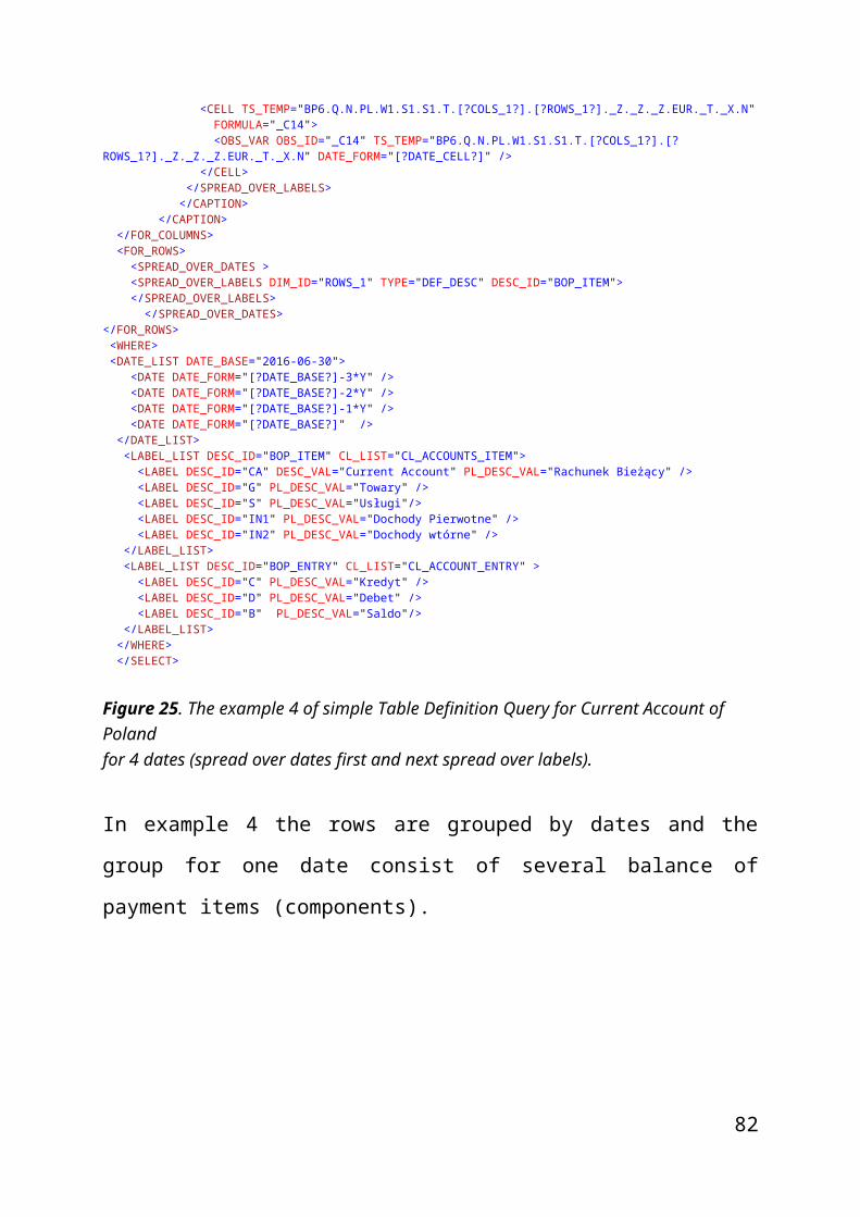
Figure 37. The input file TDQ_5_BOP_CA.xml has been pointed.

Step 4:

Log-in to the connection with Statistical Data Warehouse ESCB using IAM login.

Figure 38. The window for Log in.

Step 5:

Waite a moment until application process the query.

82

Figure 39. The Excel Result Data Table for query TDQ_BOB_5_CA.xml. The name of the output file is Excel_TDQ_5_BOP_CA.xlsx.

Step 6:

Find the files produced by the application:

- Req_TDQ_5_BOP_CA.xml,- Result_TDQ_5_BOP_CA.xml,- Excel_TDQ_5_BOP_CA.xlsx,- Result_TDQ_5_BOP_CA.pdf

and additional file containing list of imported observations

- sdw_ws_TDQ_5_BOP_CA.xml.

In order to have HTML presentation of the files:

- Req_TDQ_5_BOP_CA.xml,- Result_TDQ_5_BOP_CA.xml,

one should apply the xslt style sheets (in current example TDQ_Result.xsl, NBP_logo_zielone_RGB_WWW.png).

83

VI.3. List of files.

All files should be copied into one directory.

Application file is:

TDQ_ESCB_V0_1.xlsm

The following examples of input Table Definition Queries were prepared:

- TDQ_1_BOP_CA.xml,- TDQ_2_BOP_CA.xml,- TDQ_3_BOP_CA.xml,- TDQ_4_BOP_CA.xml,- TDQ_5_BOP_CA.xml,- TDQ_6_BOP_CA.xml,- TDQ_7_BOP_CA.xml,- TDQ_8_BOP_CA.xml,- TDQ_9_BOP_CA.xml,- TDQ_10_BOP_IIP.xml,- TDQ_11_BOP_IIP.xml,- TDQ_12_BOP_IIP.xml,

The style sheets file (to convert to HTML) are:

- TDQ_Result.xsl for English language presentation- TDQ_PL_Result.xsl for Polish language presentation.

The file containing logo of National bank of Poland:

- NBP_logo_zielone_RGB_WWW.png

84

Introduction · Web viewEach statistical process: Starts with sending the request file with...

Documents

Transcript of Introduction · Web viewEach statistical process: Starts with sending the request file with...