Introduction - TUM

Introduction

Contents

Parametric curves 10

Power basis form of a curve 11

10 INTRODUCTION

Among the different representations to describe a quarter of circle(of radius 1 and centered at the origin), one can use an implicit formusing the equation

f (x, y) := x2 + y2 − 1 = 0, x ≥ 0 and y ≥ 0

In practice, implicit forms are well adapted for unbounded geome-tries. On the other hand, given a point, it is easy to determine if it ison the curve or a surface. Although, this is an important question, ingeneral, we are interested in geometric manipulations in CAD sys-tems, such as improving the resolution, smoothness and having localcontrol of a given curve or surface. These properties are very difficultto ensure when using an implicit form; at the end, a computer needsdiscrete values in order to plot or manipulate a CAD object, which isin opposition with the analytical form represented by an equation.

Parametric curves

Another way of representing a quarter of circle is to consider theparametric curve define in 1, where θ ∈

�0, π

2�

C(θ) =�

x(θ)y(θ)

�=

�cos θ

sin θ

�(1)

Figure 1: Quarter of circle of radius 1,using polar coordinates.

in which case we can compute its derivative as

C �(θ) =

�− sin θ

cos θ

�(2)

The tangent at θ = 0 and θ = π2 are then given by C �(θ := 0) =

�01

�

and C �(θ := π2 ) =

�−10

�.

Another way to represent the quarter of circle, is to introduce thevariable t := tan θ

2 , then we get the following rational form 3, wheret ∈ [0, 1],

C(t) =�

x(t)y(t)

�=

�1−t2

1+t22t

1+t2

�(3)

Exercise 1 Compare the CPU cost for an evaluation for the presentedrepresentations.

There are different advantages for having a parametric form:

• Extending a 2D curve to 3D,

• Ideal for bounded curves and surfaces,

POWER BASIS FORM OF A CURVE 11

• Natural orientation of curves and surfaces,

• Appropriate representation for design on a computer. In someparticular cases, the coefficients in a parametric form possess inter-esting geometric significance,

• Computing a point on a curve is easy, while finding its parametricvalue is a in general a non-linear problem,

Remark 1 Notice that in some cases, this representation may introducesingularities that are unrelated to the described geometry.

Remark 2 Computing the derivatives (tangent or normal vectors at theextremeties) needs an evaluation. We shall be more interested in representa-tion where such informations can be extracted directly from the parametricrepresentations.

Although one can use any parametric representation for CADsystems, it is important to restrict to a representation that is

• capable of reproducing a wild class of curves/surfaces

• easy to implement

• efficient and accurate evaluation

• numerical stable evaluation

• easy evaluation of points and their derivatives

• evaluation complexity of the same or comparable order as polyno-mials

• small memory storage

Power basis form of a curve

If we restrict our representation to polynomials, one naive way wouldbe to use power basis, i.e. monomials as in 4

C(t) =n

∑i=0

aiti (4)

where ai =

axi

ayi

azi

are 2D or 3D vectors.

Using the Taylor expansion, we get C �(t)|t=0 = i!ai, which leads toai =

C �(t)|t=0i! . We then have a direct access to the derivative at t = 0,

but only at this point.

12 INTRODUCTION

The evaluation of such a form can be done using the Horner algo-rithm as described in 5:

C(t) = a0 + t (a1 + t (a2 + t (· · ·+ t (an−1 + tan)))) (5)

Exercise 2 Compute the CPU cost for the Horner algorithm.

Exercise 3 Write a Python implementation for the Horner algorithm.

Exercise 4 (Parallel evaluation) Let us consider a polynomial P of degreen, defined as P(t) = ∑n

i=0 aiti. Using the form

P(t) =k−1

∑j=0

xjPj(xk)

as a splitting into k independent parts, write a Python code for the parallelevaluation and compute its complexity.

Remark 3 The use of power basis form is not suited for shape and ge-ometric design; the coefficients do not have any geoemtric meaning andmodifying them do not allow for a good control of a curve or a surface,

Bézier curves

Contents

Bernstein polynomials 14

Bézier curves 15

Rational Bézier curves 17

Composite Bézier curves 18

14 BÉZIER CURVES

Bernstein polynomials

In 1885, Weierstrass proved that the set of polynomial functions on[0, 1] is dense in C ([0, 1]). In 1912, Sergei Bernstein gave a simpleproof to this result by introducing the now-famous Bernstein polyno-mials 6:

Bnk (x) =

�nk

�xk(1 − x)n−k, where k ∈ [0, n] and x ∈ [0, 1] (6)

In figure Fig. 2, we plot Bernstein polynomials of degrees 1 to 5.From these plots, we see that Bernstein polynomials are positive, thefirst and last polynomials are equal to 1 on the 0 and 1 respectivaly.More properties will be discussed in the sequel.

Figure 2: Bernstein polynomials ofdegree n = 1, 2, 3, 4, 5.

Properties of Bernstein polynomials

• Bnk (x) ≥ 0, for all k ∈ [0, n] and x ∈ [0, 1] [positivity]

• ∑nk=0 Bn

k (x) = 1, for all x ∈ [0, 1] [partition of unity]

• Bn0 (0) = Bn

n(1) = 1

BÉZIER CURVES 15

• Bnk has exactly one maximum on the interval [0, 1], at k

n

•�

Bnk (x)

�0≤k≤n is symmetric with respect to x = 1

2 [symmetry]

• Bernstein polynomials can be defined recursively using the formu-lae 7

Bnk (x) = (1 − x)Bn−1

k (x) + xBn−1k−1 (x) (7)

where we assume Bnk (x) = 0 is k < 0 or k > n

Figure 3: General evaluation triangulardiagram for a Bernstein polynomials.

• Bernstein derivatives can be computed using the formulae 8

Bnk�(x) = n

�Bn−1

k−1 (x)− Bn−1k (x)

�(8)

using the same assumption as before.

Exercise 5 Show all Bernstein properties.

Bézier curves

Rather than taking the power basis as in 4, Pierre Bézier used Bern-stein polynomials, in the 1960s while working at Renault. This leadsto the following definition of a polynomial curve 14

C(t) =n

∑k=0

PkBnk (t) (9)

The vector coefficients (P)0≤k≤n are called Bézier points or controlpoints. The reason for this will become clear in the sequel.

Examples

Example 1. A linear (n = 1) Bézier curve (fig. 4) is defined as

C(t) = P0B10(t) + P1B1

1(t)

which describes a straight line from P0 to P1, since B10(t) = 1 − t

and B11(t) = t.

Figure 4: Example of a linear Béziercurve.

Example 2. A quadratic (n = 2) Bézier curve (fig. 5) is defined as

C(t) = (1 − t)2P0 + 2t(1 − t)P1 + t2P2

Figure 5: Example of a quadratic Béziercurve.

We remark that

- the curve starts at P0 and ends at P2,

- the curve does not pass through the point P1,

16 BÉZIER CURVES

- the tangent directions to the curves at its extremeties are paral-lel to P1 − P0 and P2 − P1,

- the curve is contained in the polygone (triangle) formed byP0P1P2. This polygone is called the control polygon and it ap-proximates the shape of the curve.

Example 3. A cubic (n = 3) Bézier curve (figures 6,7,8) is defined as

C(t) = (1 − t)3P0 + 3t(1 − t)2P1 + 3t2(1 − t)P2 + t3P3

Figure 6: Example of a cubic Béziercurve.



We remark that

- the curves start at P0 and end at P3,

- the curves do not pass through the points P1 and P2,

- the tangents directions to the curves at their extremeties areparallel to P1 − P0 and P3 − P2,

- the control polygons approximate the shape of the curves,

- the curves follow the orientation of the control polygons,

- the curves are contained in the convex hulls of their controlpolygons (convex hull property).

Derivatives of a Bézier curveUsing the formulae 8, we have

C �(t) =n

∑k=0

PkBnk�(t) =

n

∑k=0

nPk

�Bn−1

k−1 (x)− Bn−1k (x)

�

by reordering the indices, we get 10

C �(t) =n−1

∑k=0

n (Pk+1 − Pk) Bn−1k (t) (10)

Therefor, we get the direct acces to the first order derivatives at theextremeties of a Bézier curve using the formulae 11

C �(0) = n (P1 − P0)

C �(1) = n (Pn − Pn−1)(11)

Second derivatives can also be computed directly from the controlpoints using the formulae 12

C ��(0) = n(n − 1) (P0 − 2P1 + P2)

C ��(1) = n(n − 1) (Pn − 2Pn−1 + Pn−2)(12)

RATIONAL BÉZIER CURVES 17

Properties of Bézier curvesBecause of the symmetry of the Bernstein polynomials, we have

• ∑nk=0 PkBn

k = ∑nk=0 PkBn

n−k

Thanks to the interpolation property, for Bn0 and Bn

n , of the Bernsteinpolynomials at the endpoints, we get

• C(0) = P0 and C(1) = Pn

Using the partition unity property of the Bernstein polynomials, weget

• any point C(t) is an affine combination of the control points

Therefor,

• Bézier curves are affinely invariant; i.e. the image curve Φ(∑nk=0 PkBn

k )

of a Bézier curve, by an affine mapping Φ, is the Bézier curve hav-ing (Φ(Pi))0≤i≤n as control points.

due to the partition unity of the Bernstein polynomials and theirnon-negativity,

• any point C(t) is a convex combination of the control points

finally, we get the convex hull property,

• A Bézier curve lies in the convex hull of its control points

Rational Bézier curves

We first introduce the notion of Rational Bernstein polynomials de-fined as, and wi > 0, ∀i ∈ [0, n]

Rnk (t) :=

wiBnk (t)

∑ni=0 wiBn

i (t)(13)

Properties of Rational Bernstein polynomials

• Rnk (x) ≥ 0, for all k ∈ [0, n] and x ∈ [0, 1] [positivity]

• ∑nk=0 Rn

k (x) = 1, for all x ∈ [0, 1] [partition of unity]

• Rn0 (0) = Rn

n(1) = 1

• Rnk has exactly one maximum on the interval [0, 1],

• Bernstein polynomials are Rational Bernstein polynomials whenall weights are equal

Definition 1 (Rational Bézier curve)

C(t) =n

∑k=0

PkRnk (t) (14)

where Rnk (t) := wi Bn

k (t)∑n

i=0 wi Bni (t)

and wi > 0, ∀i ∈ [0, n]

18 BÉZIER CURVES

Examples

Example 1. We consider the quadratic Rational Bézier curve,

Figure 9: Circular arc using quadraticRational Bézier curve.

where the weights are given by w0 = 1, w1 = 1 and w2 = 2 and the

control points are P0 =

�10

�, P1 =

�11

�and P2 =

�01

�.

This leads to a representation of the circular arc, using the para-

metric form C(t) =�

1−t2

1+t22t

1+t2

�.

Composite Bézier curves

A composite Bézier curve is a piecewise Bézier curve that is at leastcontinuous at the interpolant control points. An example is givenin Fig. 10. The global curve inherit all the nice properties of Béziercurves however, it has a major drawback: when moving an inter-polant control point, we must ensure that the associated regularity isnot broken, unless it is what we want. This means that a good repre-sentation of a curve needs to have the locality control through controlpoints, but also the control points must be associated to some givenregularity.

Figure 10: A composite Bézier curveusing 3 quadratic Bézier curves.

Since Bernstein polynomials are defined locally on the interval [0, 1],and they do not encode any global redularity of the curve, we needanother representation, in terms of other functions, while keepingin mind that these functions must be polynomials on every sub-interval. Such representation is provided by the Schoenberg spaces,for which B-Splines form a basis. In the next chapter, we will firstintroduce the uniform Splines, also known as Cardinal Splines, showtheir advantages and limitations, then we will introduce the generaldefinition of B-Splines.

B-Splines

Contents

Knot vector families 20

Examples 22

B-Splines properties 27

Derivatives of B-Splines 30

20 B-SPLINES

In general, one needs to design curves with given regularities atsome specific locations. For this purpose, rather than consideringpiecewise Bézier curves with additional constraints on the controlpoints, we can enforce these constraints on a given space of functions.The Schoenberg spaces [1946] are perfect for this purpose. Before giv-ing more details about Schoenberg spaces, which will be covered inthe Approximation Theory part, let us for the moment, use a formaldefinition, as the following: given a subdivision {x0 < x1 < · · · < xr}of the interval I = [x0, xr], the Schoenberg space is the space of piece-wise polynomials of degree p, on the interval I and given regularities{k1, k2, · · · , kr−1} at the internal points {x1, x2, · · · , xr−1}.

Given m and p as natural numbers, let us consider a sequenceof non decreasing real numbers T = {ti}0�i�m. T is called knotssequence. From a knots sequence, we can generate a B-splines familyusing the reccurence formula 15.

Definition 2 (B-Splines using Cox-DeBoor Formula) The j-th B-spline of degree p is defined by the recurrence relation:

Npj =

t − tj

tj+p − tjNp−1

j +tj+p+1 − t

tj+p+1 − tj+1Np−1

j+1 , (15)

whereN0

j (t) = χ[tj ,tj+1[(t)

for 0 ≤ j ≤ m − p − 1.

Remark 4 When working with Bernstein polynomials, we introduced theconvention Bn

i = 0 for all i < 0 or i > n. For B-Splines, we have a similarconvetion Np

j = 0 if j < 0 or j > n. In addition, we also assume 00 = 0,

when using the formula 15 and N0j = 0 if tj = tj+1.

Remark 5 k = p + 1 is called the order of the B-Splines.

Figure 11: General evaluation triangulardiagram for a B-Spline.

In figure Fig. 12, we plot the quadratic B-Splines functions associ-ated to the knots sequence {0, 0, 0, 1, 2, 2, 3, 4, 5, 5, 5}. As we can see,there are 8 B-Splines functions and we recover the interpolation prop-erty at the first and last knot. In addition, while all the B-Splines aresmooth at the internal knots, N2

3 is only C0 at the grid point 2.Now if we look for the cubic B-Splines that are associated to the sameknots sequence {0, 0, 0, 1, 2, 2, 3, 4, 5, 5, 5}, we see that the interpolationproperty is no longer true 13.

Knot vector families

There are two kind of knot vectors, called clamped and unclamped.Both families contains uniform and non-uniform sequences. In figure

KNOT VECTOR FAMILIES 21

Figure 12: Quadratic B-Splines gen-erated using the knots sequence{0, 0, 0, 1, 2, 2, 3, 4, 5, 5, 5}.

Figure 13: Cubic B-Splines gen-erated using the knots sequence{0, 0, 0, 1, 2, 2, 3, 4, 5, 5, 5}.

Fig. 14, we show examples of clamped uniform knots. Fig. 15, weshow examples of clamped non-uniform knots, while figures Fig. 16and Fig. 17 are examples of unclamped knots sequences for uniformand non-uniform cases, respectively.The special case of clamped sequences, where the first and the last

22 B-SPLINES

knots are repeated p + 1 times exactly is known as open knot vector.

Figure 14: Clamped uniformknots (left) quadratic B-Splines us-ing T = {0, 0, 0, 1, 2, 3, 4, 5, 5, 5},(right) quadratic B-Splines usingT = {−0.2,−0.2, 0.0, 0.2, 0.4, 0.6, 0.8, 0.8}.

Figure 15: Clamped non-uniformknots (left) quadratic B-Splinesusing T = {0, 0, 0, 1, 3, 4, 5, 5, 5},(right) quadratic B-Splines usingT = {−0.2,−0.2, 0.4, 0.6, 0.8, 0.8}.

Figure 16: Unclamped uniformknots (left) quadratic B-Splinesusing T = {0, 1, 2, 3, 4, 5, 6, 7, 8},(right) quadratic B-Splines usingT = {−0.2, 0.0, 0.2, 0.4, 0.6, 0.8, 1.0}.

Figure 17: Unclamped non-uniformknots (left) quadratic B-Splinesusing T = {0, 0, 3, 4, 7, 8, 9},(right) quadratic B-Splines usingT = {−0.2, 0.2, 0.4, 0.6, 1.0, 2.0, 2.5}.

Examples

Before stating some B-Splines properties, let us take a look to someexamples.

Example 1. Let T = {0, 1, 2} and p = 1.

Figure 18: Evaluation diagram forexamples 1, 2 and 3.

We first compute the B-Splines of degrees 0

N00 =

1, 0 ≤ t < 1

0, otherwise

N01 =

1, 1 ≤ t < 2

0, otherwise

EXAMPLES 23

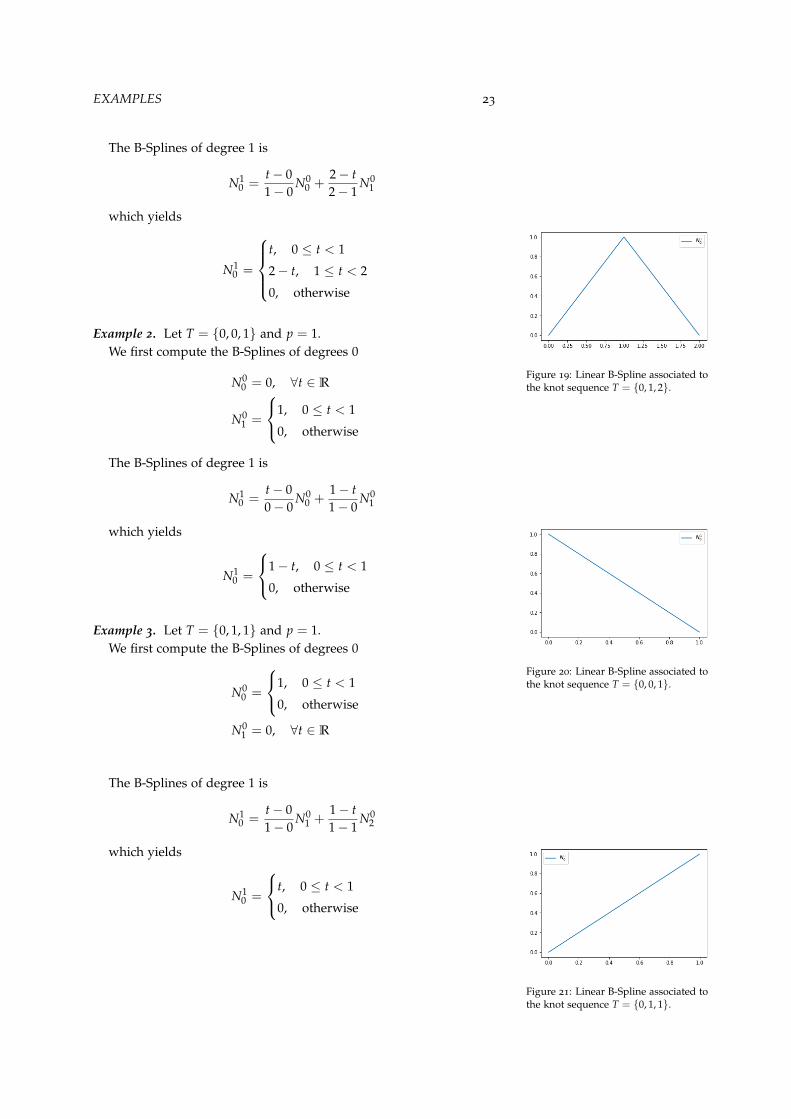
The B-Splines of degree 1 is

N10 =

t − 01 − 0

N00 +

2 − t2 − 1

N01

which yields

N10 =

t, 0 ≤ t < 1

2 − t, 1 ≤ t < 2

0, otherwise

Figure 19: Linear B-Spline associated tothe knot sequence T = {0, 1, 2}.

Example 2. Let T = {0, 0, 1} and p = 1.We first compute the B-Splines of degrees 0

N00 = 0, ∀t ∈ R

N01 =

1, 0 ≤ t < 1

0, otherwise


N10 =

t − 00 − 0

N00 +

1 − t1 − 0

N01

which yields

N10 =

1 − t, 0 ≤ t < 1

0, otherwise


Example 3. Let T = {0, 1, 1} and p = 1.We first compute the B-Splines of degrees 0

N00 =

1, 0 ≤ t < 1

0, otherwise

N01 = 0, ∀t ∈ R


N10 =

t − 01 − 0

N01 +

1 − t1 − 1

N02

which yields

N10 =

t, 0 ≤ t < 1

0, otherwise


24 B-SPLINES

Example 4. Let T = {0, 0, 1, 1} and p = 1.

Figure 22: Evaluation diagram forexamples 4 and 5.

In the examples 2 and 3 we computed the linear B-Splines asso-ciated to the knots sequences {0, 0, 1} and {0, 1, 1}. Then we getimmediatly that the knots sequens {0, 0, 1, 1} will exactly generatethe same B-Splines, i.e.

N10 =

1 − t, 0 ≤ t < 1

0, otherwise

N11 =

t, 0 ≤ t < 1

0, otherwise

Figure 23: Linear B-Splines associatedto the knots sequence T = {0, 0, 1, 1}.

Example 5. Let T = {0, 0, 1, 2} and p = 1.In the examples 2 and 1 we computed the linear B-Splines asso-ciated to the knots sequences {0, 0, 1} and {0, 1, 2}. Then we getimmediatly that the knots sequens {0, 0, 1, 2} will exactly generatethe same B-Splines, i.e.

N10 =

1 − t, 0 ≤ t < 1

0, otherwise

N11 =

t, 0 ≤ t < 1

2 − t, 1 ≤ t < 2

0, otherwise

Figure 24: Linear B-Splines associatedto the knot sequence T = {0, 0, 1, 2}.

EXAMPLES 25

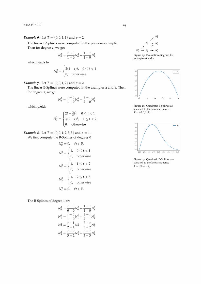
Example 6. Let T = {0, 0, 1, 1} and p = 2.

Figure 25: Evaluation diagram forexamples 6 and 7.

The linear B-Splines were computed in the previous example.Then for degree 2, we get

N20 =

t − 01 − 0

N10 +

1 − t1 − 0

N11

which leads to

N20 =

2(1 − t)t, 0 ≤ t < 1

0, otherwise

Figure 26: Quadratic B-Splines as-sociated to the knots sequenceT = {0, 0, 1, 1}.

Example 7. Let T = {0, 0, 1, 2} and p = 2.The linear B-Splines were computed in the examples 2 and 1. Thenfor degree 2, we get

N20 =

t − 01 − 0

N10 +

2 − t2 − 0

N11

which yields

N20 =

2t − 32 t2, 0 ≤ t < 1

12 (2 − t)2, 1 ≤ t < 2

0, otherwise

Figure 27: Quadratic B-Splines as-sociated to the knots sequenceT = {0, 0, 1, 2}.

Example 8. Let T = {0, 0, 1, 2, 3, 3} and p = 1.We first compute the B-Splines of degrees 0

N00 = 0, ∀t ∈ R

N01 =

1, 0 ≤ t < 1

0, otherwise

N02 =

1, 1 ≤ t < 2

0, otherwise

N03 =

1, 2 ≤ t < 3

0, otherwise

N04 = 0, ∀t ∈ R

The B-Splines of degree 1 are

N10 =

t − 00 − 0

N00 +

1 − t1 − 0

N01

N11 =

t − 01 − 0

N01 +

2 − t2 − 1

N02

N12 =

t − 12 − 1

N02 +

3 − t3 − 2

N03

N13 =

t − 23 − 2

N03 +

3 − t3 − 3

N04

26 B-SPLINES

which gives

N10 =

1 − t, 0 ≤ t < 1

0, otherwise

N11 =

t, 0 ≤ t < 1

2 − t, 1 ≤ t < 2

0, otherwise

N12 =

t − 1, 1 ≤ t < 2

3 − t, 2 ≤ t < 3

0, otherwise

N13 =

t − 2, 2 ≤ t < 3

0, otherwise

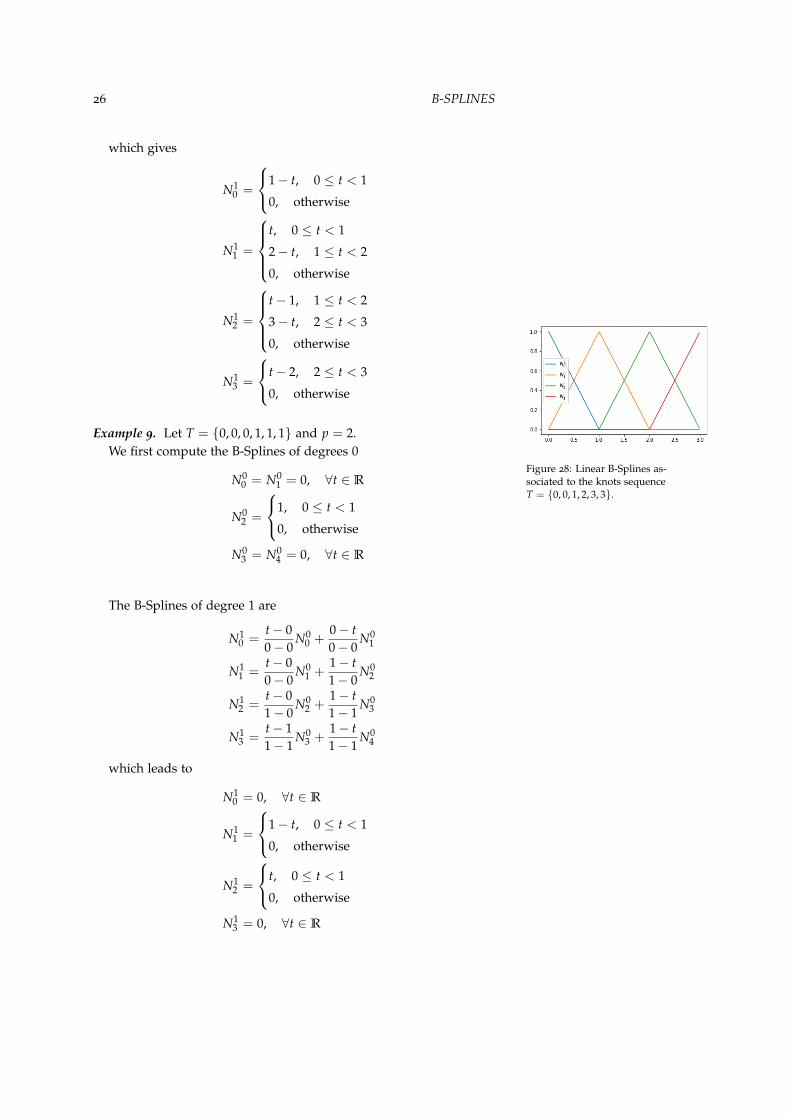
Figure 28: Linear B-Splines as-sociated to the knots sequenceT = {0, 0, 1, 2, 3, 3}.

Example 9. Let T = {0, 0, 0, 1, 1, 1} and p = 2.We first compute the B-Splines of degrees 0

N00 = N0

1 = 0, ∀t ∈ R

N02 =

1, 0 ≤ t < 1

0, otherwise

N03 = N0

4 = 0, ∀t ∈ R


N10 =

t − 00 − 0

N00 +

0 − t0 − 0

N01

N11 =

t − 00 − 0

N01 +

1 − t1 − 0

N02

N12 =

t − 01 − 0

N02 +

1 − t1 − 1

N03

N13 =

t − 11 − 1

N03 +

1 − t1 − 1

N04

which leads to

N10 = 0, ∀t ∈ R

N11 =

1 − t, 0 ≤ t < 1

0, otherwise

N12 =

t, 0 ≤ t < 1

0, otherwise

N13 = 0, ∀t ∈ R

B-SPLINES PROPERTIES 27


N20 =

t − 00 − 0

N10 +

1 − t1 − 0

N11

N21 =

t − 01 − 0

N11 +

1 − t1 − 0

N12

N22 =

t − 01 − 0

N12 +

1 − t1 − 1

N13

which leads to

N20 =

(1 − t)2, 0 ≤ t < 1

0, otherwise

N21 =

2t(1 − t), 0 ≤ t < 1

0, otherwise

N22 =

t2, 0 ≤ t < 1

0, otherwise

In this case, we recover the Bernstein polynomials of degree 2.

Figure 29: Linear B-Splines as-sociated to the knots sequenceT = {0, 0, 0, 1, 1, 1}.

Exercise 6 Compute the B-Splines generated by the knots sequences:

- T = {0, 0, 0, 1, 2, 2, 3, 4, 5, 5, 5} with p = 2

- T = {0, 1, 2, 2, 3, 4, 5, 5, 6} with p = 2

B-Splines properties

B-Splines have many interesting properties that are listed below. Ingeneral, most of the proofs are done by induction on the B-Splinedegree.

Proposition 1 B-splines are piecewise polynomial of degree p

Proof. We proceed by induction. When p = 0, B-Splines are either the0 or the characteristic functions, which are constant polynomials. Forp = 1, the Cox-DeBoor formula shows that the generated B-Splinesare piecewise linear functions, because of the weights that multplythe constant functions (B-Splines of degree p = 0).Now assume that B-Splines of degree p − 1 are piecewise polynomi-als of degree p − 1. Again using the Cox-DeBoor formula, we see thatthe degree will be increased by 1 because of the linear weights, oneach sub-interval. This completes the proof.

Remark 6 The B-splines functions associated to open knots sequenceswithout internal knots, i.e. the length of the knots sequence is exactly 2p +

2, are the Bernstein polynomials of degreep.

28 B-SPLINES

Proposition 2 (compact support) Npj (t) = 0 for all t /∈ [tj, tj+p+1).

Proof. By taking a look at the triangular diagram 11 for the evalua-tion of the jth B-Spline of degree p. We see that Np

j depends only on

the B-Splines {N0j , N0

j+1, · · · , N0j+p}. The laters are exactly the charac-

teristic functions on the intervals [ti, ti+1), ∀i ∈ {j, j + 1, · · · , j + p}.Therefor, Np

j (t) = 0, for all t /∈ [tj, tj+p+1).

Proposition 3 If t ∈ [tj, tj+1), then only the B-splines {Npj−p, · · · , Np

j }are non vanishing at t.

Proof. Using the last proposition, the support of Npi is defined as

supp�

Npi

�= [ti, ti+p+1) for every i ∈ {j − p, · · · , j}. Therefor,

on the interval [tj, tj+1) =�

j−p≤i≤jsupp

�Np

i

�, only the B-Splines

{Npj−p, · · · , Np

j } are non-zeros.

Proposition 4 (non-negativity) Npj (t) ≥ 0, ∀t ∈ [tj, tj+p+1)

Proof. This can be proved by induction. It is true for p = 0, sinceall B-Splines are either 0 or the characteristic function. Assume theproperty holds for p − 1, using the Cox-DeBoor formula we have:

Npj =

x − tj

tj+p − tjNp−1

j +tj+p+1 − x


j+1

since, t ∈ [tj, tj+p+1), we havex−tj

tj+p−tj≥ 0 and

tj+p+1−xtj+p+1−tj+1

≥ 0 when-ever tj+p > tj and tj+p+1 > tj+1, otherwise these terms are identicalyequal to 0, by convention.

On the other hand, Np−1j ≥ 0 and Np−1

j+1 ≥ 0. Therefor there linearcombination is also positive.

Proposition 5 (Partition of unity) ∑ Npi (t) = 1, ∀t ∈ R

Remark 7 The previous sum ∑ Npi (t) has a meaning since for every t ∈

R, only p + 1 B-Splines are non-vanishing.

Proof. We prove this result by induction again. For p = 0, the prop-erty is true. Now let us assume it is true for p − 1.

Let j denotes the span of t. We know that ∑ Npi (t) =

j∑

i=j−pNp

i (t).

Now, using the Cox-DeBoor formula, we have

j

∑i=j−p

Npi (t) =

j

∑i=j−p

�t − ti

ti+p − tiNp−1

i (t) +ti+p+1 − t

ti+p+1 − ti+1Np−1

i+1 (t)

�

by changing the summation index in the second part, we get

j

∑i=j−p

Npi (t) =

j

∑i=j−p

t − titi+p − ti

Np−1i (t) +

j+1

∑i=j−p+1

ti+p − tti+p − ti

Np−1i (t)

B-SPLINES PROPERTIES 29

On the other hand, we know that the only B-Splines of degree p − 1that are non-vanishing on the interval [tj, tj+1) are {Np−1

j−p+1, · · · , Np−1j },

meaning that Np−1j−p = Np−1

j+1 = 0. Therefor,

j

∑i=j−p

Npi (t) =

j

∑i=j−p+1

�t − ti

ti+p − ti+

ti+p − tti+p − ti

�Np−1

i (t)

hence,

j

∑i=j−p

Npi (t) =

j

∑i=j−p+1

Np−1i (t)

Finaly, we use the induction assumtion to complete the proof.

Remark 8 For the sake of simplicity, we shall avoid using summationindices on linear expansion of B-Splines.

Lemma 1

∑ ajNpj = ∑

�tj+p − ttj+p − tj

aj−1 +t − tj

tj+p − tjaj

�Np−1

j (16)

Proof. Using the Cox-DeBoor formula, we have

∑ ajNpj = ∑

�aj

t − tj

tj+p − tjNp−1

j + ajtj+p+1 − t


j+1

�

By changing the summation index in the second part of the righthand side, we get

∑ ajNpj = ∑ aj

t − tj

tj+p − tjNp−1

j + ∑ aj−1tj+p − ttj+p − tj

Np−1j

which yields

∑ ajNpj = ∑

�aj

t − tj

tj+p − tj+ aj−1

tj+p − ttj+p − tj

�Np−1

j

Proposition 6 (Marsden’s idenity)

(x − y)p = ∑j

ρpj (y)Np

j (x) (17)

where

ρpj (y) =

j+p

∏i=j+1

(ti − y) (18)

30 B-SPLINES

Proof. Seting aj := ρpj (y) in the lemma 1, we get

∑ ρpj (y)Np

j (x) = ∑�

tj+p − xtj+p − tj

ρpj−1(y) +

x − tj

tj+p − tjρ

pj (y)

�Np−1

j (x)

on the other hand, by introducing αp−1j =

j+p−1∏

i=j+1(ti − y), we have

tj+p − xtj+p − tj

ρpj−1(y) +

x − tj

tj+p − tjρ

pj (y) = α

p−1j

�tj+p − xtj+p − tj

(tj − y) +x − tj

tj+p − tj(tj+p − y)

�

= (x − y)ρp−1j (y)

Therefor,

∑ ρpj (y)Np

j (x) = (x − y)∑ ρp−1j (y)Np−1

j (x)

By repeating the same computation p − 1 times (one can also use aninduction for this), we get the desired result.

Thanks to Marsden’s identity and the proposition 3, we now areable to prove the local linear independence of the B-Splines basisfunctions.

Proposition 7 (Local linear independence) On each interval [tj, tj+1),the B-Splines are lineary independent.

Proof. On the interval [tj, tj+1), there are only p + 1 non-vanishingB-Splines. On the other hand, these B-Splines reproduce polynomi-als, thanks to the Marsden’s identity. Hence, {Np

j−p, · · · , Npj } are a

basis for polynomials of degree at most p, and are therefor, linearyindependent.

Remark 9 We will see in the Approximation theory part, that the B-Splines family has also a global linear independence property.

Derivatives of B-Splines

The derivative of B-Splines can be computed reccursivly by derivingthe formula 15, which gives

Proposition 8

Npj�=

ptj+p − tj

Np−1j − p


j+1 (19)

Proof. We prove this by induction on p.For p = 1, Np−1

j and Np−1j+1 are either 0 or 1, then Np

j�

is either1

tj+1−tjor − 1

tj+2−tj+1.

DERIVATIVES OF B-SPLINES 31

Now assume that 19, is true for p − 1, where p > 1. Deriving theCox-DeBoor formula leads to

Npj�=

1tj+p − tj

Np−1j +

t − tj

tj+p − tjNp−1

j�

− 1tj+p+1 − tj+1

Np−1j+1 +

tj+p+1 − ttj+p+1 − tj+1

Np−1j+1

�

Using the induction assumption on Np−1j

�and Np−1

j+1�

and subtitutingin the last equation yields

Npj�=

1tj+p − tj

Np−1j − 1


j+1

+t − tj

tj+p − tj

�p − 1

tj+p−1 − tjNp−2

j − p − 1tj+p − tj+1

Np−2j+1

�

+tj+p+1 − t

tj+p+1 − tj+1

�p − 1

tj+p − tj+1Np−2

j+1 − p − 1tj+p+1 − tj+2

Np−2j+2

�

=1

tj+p − tjNp−1

j − 1tj+p+1 − tj+1

Np−1j+1

+p − 1

tj+p − tj

t − tj


j

+p − 1

tj+p − tj+1

�tj+p+1 − t

tj+p+1 − tj+1− t − tj

tj+p − tj

�Np−2

j+1

− p − 1tj+p+1 − tj+1

tj+p+1 − ttj+p+1 − tj+2

Np−2j+2

Since,

tj+p+1 − ttj+p+1 − tj+1

− t − tj

tj+p − tj=

tj+p − ttj+p − tj

− t − tj+1

tj+p+1 − tj+1

we get

Npj�=

1tj+p − tj

Np−1j − 1


j+1

+p − 1

tj+p − tj

�t − tj


j +tj+p − ttj+p − tj

Np−2j+1

�

− p − 1tj+p+1 − tj+1

�t − tj+1

tj+p − tj+1Np−2

j+1 +tj+p+1 − t


j+2

�

By applying the Cox-DeBoor formula for Np−1j and Np−1

j+1 we get thedesired result.

Exercise 7 Show that the r-th derivative of Npj is given by

Npj(r)

=p

tj+p − tjNp−1

j(r−1) − p


j+1(r−1)

Cardinal B-Splines

Contents

Cardinal B-Splines 34

Cardinal B-Splines properties 36

Cardinal B-Spline series 38

Scaled and translated Cardinal B-Splines 38

Cardinal Splines 38

34 CARDINAL B-SPLINES

Cardinal B-Splines

Cardinal B-Splines play an important role in the approximation the-ory (multi-resolution approximation, . . . ). In the sequel, we shall givea definition of the Cardinal B-Spline using the convolution operator.Then, we will present some of the most important properties, at leastneeded when using uniform B-Splines in a Finite Elements method.

Definition 3 A cardinal B-spline of zero degree, denoted by φ0, is thecharacteristic function over the interval [0, 1), i.e.,

φ0(t) :=

�1, t ∈ [0, 1)0, otherwise

(20)

A cardinal B-Spline of degree p, p ∈ N, denoted by φp, is defined byconvolution as

φp(t) =�φp−1 ∗ φ0

�(t) =

�

Rφp−1(t − s)φ0(s) ds (21)

Example 1: When p = 1, it is easy to show that

φ1(t) :=

t, t ∈ [0, 1)2 − t, t ∈ [1, 2)0, otherwise

(22)

When p = 2, it is easy to show that

φ2(t) :=

12 x2, t ∈ [0, 1)12 + (x − 1)− (x − 1)2, t ∈ [1, 2)12 − (x − 2) + 1

2 (x − 2)2, t ∈ [2, 3)0, otherwise

(23)

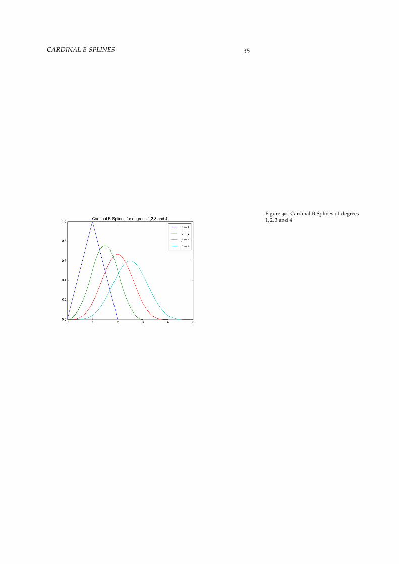
In figure (Fig. 30), we plot the Cardinal B-Splines of degrees 1, 2, 3and 4.

Remark 10 The colored area under the graph of φ2 represents the average� xx−1 φ2(t)dt which is the value φ3(x).

CARDINAL B-SPLINES 35

Figure 30: Cardinal B-Splines of degrees1, 2, 3 and 4


Cardinal B-Splines properties

Let φp be a cardinal B-Spline of degree p, p ∈ N. The followingproperties can be proved by induction on the B-Spline degree p.

Theorem 8 (Minimal support) the support of φp is [0, p + 1]

Theorem 9 (Positivity) φp(s) ≥ 0, ∀s ∈ [0, p + 1]

Theorem 10 φp ∈ C p−1

Theorem 11 φp is a piecewise-polynomial of degree p at each interval[i, i + 1], ∀i ∈ {0, 1, . . . , p}

The sequence {0, 1, 2, . . . , p} is known as the breaks of the cardinalB-Spline of degree p.

Theorem 12 ∀t ∈ [0, p + 1] and p ≥ 1, we have

φ̇p(t) = φp−1(t)− φp−1(t − 1) (24)

Theorem 13 (Symmetry) φp is symmetric on the interval [0, p + 1], i.e.

φp(t) = φp(p + 1 − t), ∀t ∈ [0, p + 1] (25)

The following theorem was proved in 1972 by both Cox and Deboorseparatly.

Theorem 14 (Cox-Deboor) ∀t ∈ [0, p + 1] and p ≥ 1, we have

φp(t) =tp

φp−1(t) +p + 1 − t

pφp−1(t − 1) (26)

Proof. Let φpi (t) := φp(t − i), ∀t ∈ [0, p + 1]. We will proof the

result by induction. Since both sides vanish at t = 0, we will use theequivalence to the formula for the derivative 12.

φp−10 − φ

p−11 =

1p

�φ

p−10 − φ

p−11

�+

�tp

�φ

p−20 − φ

p−21

�+

p + 1 − tp

�φ

p−21 − φ

p−22

��

(27)

The last term of the previous relation, can be written as

p − 1p

��t

p − 1φ

p−20 +

p − tp − 1

φp−21

�−

�t − 1p − 1

φp−21 +

p − (t − 1)p − 1

φp−22

��

(28)

CARDINAL B-SPLINES 37

Now, if we assume that the recursion is valid up to p − 1, then thelast terms is equal to

p − 1p

�φ

p−10 − φ

p−11

�(29)

For any Cardinal B-Spline of degree p, we denote by αpi =

�α

p0,i, α

p1,i, . . . , α

pp,i

�

the sequence of its mononial coefficients on [i, i + 1]

φp(t) = αp0,i + α

p1,it

2 + . . . + αpp,it

p, ∀t ∈ [i, i + 1] (30)

When i, j /∈ [0, p], we set αpi,j

Theorem 15 (Taylor Coefficients)

αpl,k =

kp

αp−1l,k +

1p

αp−1l−1,k +

p + 1 − kp

αp−1l,k−1 −

1p

αp−1l−1,k−1 (31)

Proof. Using the Cox-Deboor theorem (14), if x = i + t where t ∈[0, 1], we have

xp

φp−1(x) =�

kp+

tp

��α

p−10,i−1 + α

p−11,i−1t2 + . . . + α

p−1p,i−1tp

�

p + 1 − xp

φp−1(x − 1) =�

p + 1 − kp

− tp

��α

p−10,i−1 + α

p−11,i−1t2 + . . . + α

p−1p,i−1tp

�

Adding the last expressions together, we get the the expected relationfor α

pp,i.

Corollary 1 (Cardinal B-Splines evaluation using pp-form) Thanksto the theorem (15), we can compute analyticaly the Taylor coefficients forlow B-Splines order (Tables 1, 2 and 3).

Interval Taylor coefficients

[0, 1] 0 1 α0,1

[1, 2] 1 −1 α1,1

Table 1: The linear Cardinal B-SplineTaylor coefficients.


[0, 1] 0 0 12 α0,2

[1, 2] 12 1 −1 α1,2

[2, 3] 12 −1 1

2 α2,2

Table 2: The quadratic Cardinal B-Spline Taylor coefficients.


[0, 1] 0 0 0 16 α0,3

[1, 2] 16

12

12 − 1

2 α1,3

[2, 3] 23 0 −1 1

2 α2,3

[3, 4] 16 − 1

212 − 1

6 α1,3

Table 3: The cubic Cardinal B-SplineTaylor coefficients.

Theorem 16 (Inner product)�

Rφ(r)p (t)φ(s)

q (t + k) dt = (−1)rφ(r+s)p+q+1(p + 1 + k) = (−1)sφ

(r+s)p+q+1(q + 1 − k)

(32)


Cardinal B-Spline series

Scaled and translated Cardinal B-Splines

From now on, h > 0 will denote the mesh step. hZ is the uniformgrid of width h. The scaled and translated Cardinal B-Spline of de-gree p is defined by

φi,h,p(x) := φp

� xh− i

�(33)

The support of φi,h,p is [i, i + p + 1]h. We introduce the sequence(ti)i∈Z, where ti = ih, ∀i ∈ Z. The following result is another versionof the Cox-Deboor theorem (14).

Theorem 17 (Cox-Deboor) ∀t ∈ R and p ≥ 1, we have

φi,h,p(t) =t − ti

ti+p − tiφi,h,p−1(t) +

ti+p+1 − tti+p+1 − ti+1

φi+1,h,p−1(t) (34)

with φi,h,p(t) = 0, ∀t /∈ [ti, ti+p+1].

Proof. Using the definition of the scaled and translated CardinalB-Spline and the theorem (14), we have

φi,h,p(t) =t − ih

hpφi,h,p−1(t) +

h(p + 1 + i)− thp

φi+1,h,p−1(t) (35)

The result is straightforward, using the fact that ti+p − ti = ti+p+1 −ti+1 = hp.

Cardinal Splines

Definition 4 (Cardinal Spline) A Cardinal Spline, or cardinal B-Splineserie, of degree p on the grid hZ is the linear combination

∑k∈Z

ckφk,h,p (36)

In figure (Fig. 31), we plot all non-vanishing Cardinal B-Splines onthe interval [2, 3]. In figure (Fig. 32), we plot a Cardinal B-Splineserie.

Proposition 9 (Marsden’s identity)

∀x, t ∈ R, (x − t)p = ∑k∈Z

mk,h,p(t)φk,h,p(x) (37)

where mk,h,p(t) = hpΠpi=1

�k + i − t

h�

Proof.

CARDINAL B-SPLINE SERIES 39

Figure 31: Non-vanishing CardinalB-Splines on the interval [2, 3]

Figure 32: Example of a cubic CardinalB-Spline serie.

Proposition 10 (Partition of unity)

1 = ∑k∈Z

φk,h,p(t), ∀t ∈ R (38)

Proposition 11 (Linear independence) For any element [i, i + 1]h, theCardinal B-Splines

�φk,h,p

�i−p≤k≤i

are linearly independent.

Proposition 12 (Representation of Polynomials)

Proof.

B-Splines curves

Contents

B-Splines curves 42

Derivtive of a B-spline curve 44

Rational B-Splines (NURBS) curves 44

Modeling conics using NURBS 45

Fundamental geometric operations 48

Knot insertion 48

Degree elevation 50

42 B-SPLINES CURVES

B-Splines curves

Let (Pi)0�i�n ∈ Rd be a sequence of control points. Following thesame approach as for Bézier curves, we define B-Splines curves as

Definition 5 (B-Spline curve) The B-spline curve in Rd associated toT = (ti)0�i�n+p+1 and (Pi)0�i�n is defined by :

C(t) =n

∑i=0

Npi (t)Pi

Remark 11 The use of open knot vector leads to an interpolating curve atthe endpoints.

Examples

Example 1. We consider quadratic B-Spline curve on the knot vectorT = {0, 0, 0, 1, 1, 1}. This leads to a quadratic Bézier curve.

Figure 33: Quadratic B-Spline curveusing the knot vector T = {0, 0, 0, 1, 1, 1}

Example 2. We consider cubic B-Spline curve on the knot vectorT = {0, 0, 0, 0, 1, 1, 1, 1}. This leads to a cubic Bézier curve.

Figure 34: Cubic B-Spline curve usingthe knot vector T = {0, 0, 0, 0, 1, 1, 1, 1}

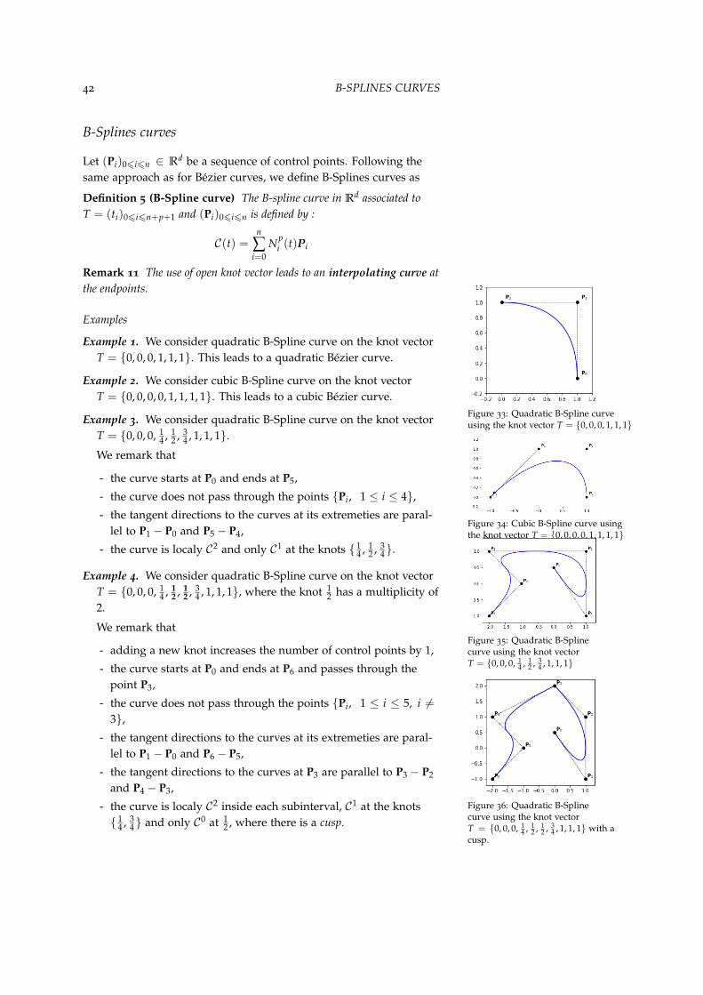
Example 3. We consider quadratic B-Spline curve on the knot vectorT = {0, 0, 0, 1

4 , 12 , 3

4 , 1, 1, 1}.

We remark that

- the curve starts at P0 and ends at P5,

- the curve does not pass through the points {Pi, 1 ≤ i ≤ 4},


- the curve is localy C2 and only C1 at the knots { 14 , 1

2 , 34}.

Figure 35: Quadratic B-Splinecurve using the knot vectorT = {0, 0, 0, 1

4 , 12 , 3

4 , 1, 1, 1}


4 , 12 , 1

2 , 34 , 1, 1, 1}, where the knot 1

2 has a multiplicity of2.


4 , 12 , 1

2 , 34 , 1, 1, 1} with a

cusp.

We remark that

- adding a new knot increases the number of control points by 1,

- the curve starts at P0 and ends at P6 and passes through thepoint P3,

- the curve does not pass through the points {Pi, 1 ≤ i ≤ 5, i �=3},


- the tangent directions to the curves at P3 are parallel to P3 − P2

and P4 − P3,

- the curve is localy C2 inside each subinterval, C1 at the knots{ 1

4 , 34} and only C0 at 1

2 , where there is a cusp.

B-SPLINES CURVES 43


4 , 12 , 1

2 , 34 , 1, 1, 1}, where the knot 1

2 has a multiplicity of2.


4 , 12 , 1

2 , 34 , 1, 1, 1} with-

out a cusp.

We remark that although the knot 12 has a multiplicity of 2, the

curve is visualy smooth. In fact, it still has the same properties asin the previous example, except that the curve is more than justC0 at the double knot 1

2 , but not C1. To be more specific, it has aregularity of G1 at the knot 1

2 .

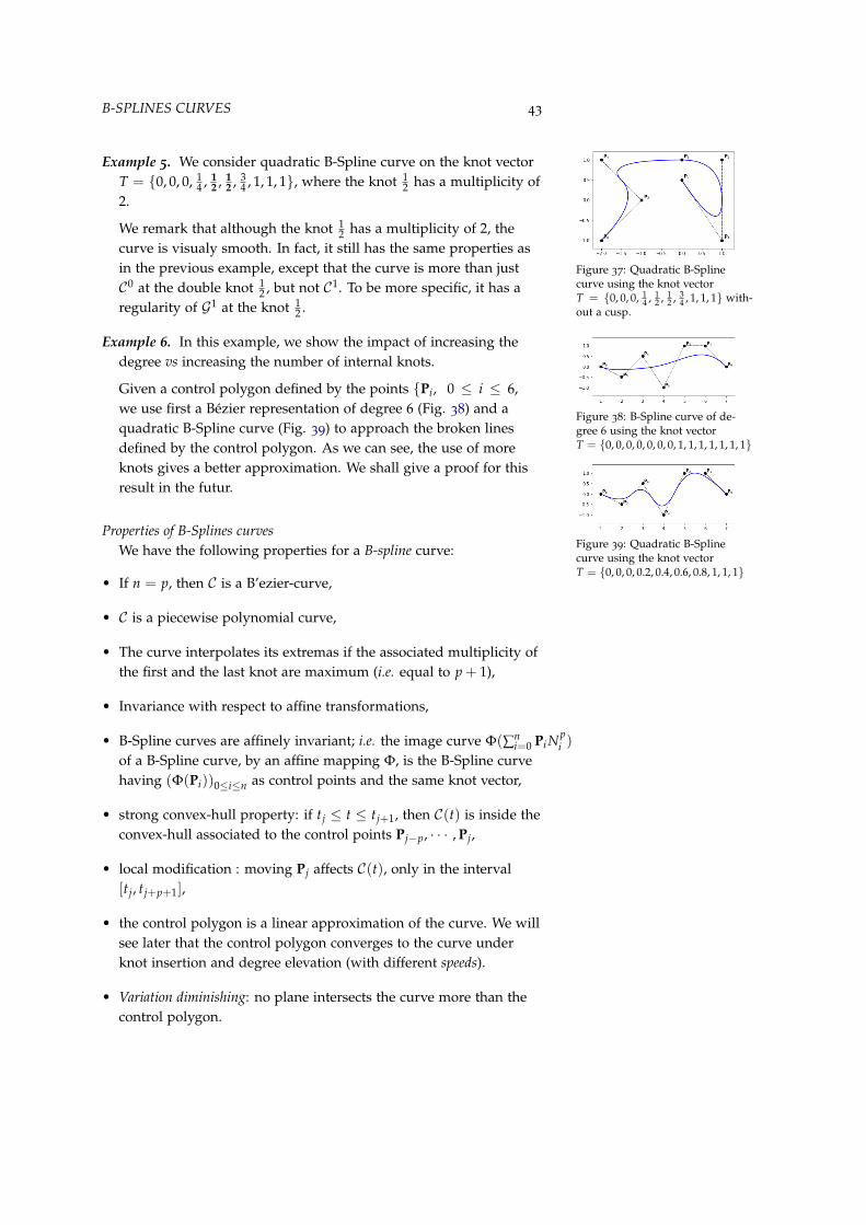
Example 6. In this example, we show the impact of increasing thedegree vs increasing the number of internal knots.

Figure 38: B-Spline curve of de-gree 6 using the knot vectorT = {0, 0, 0, 0, 0, 0, 0, 1, 1, 1, 1, 1, 1, 1}

Figure 39: Quadratic B-Splinecurve using the knot vectorT = {0, 0, 0, 0.2, 0.4, 0.6, 0.8, 1, 1, 1}

Given a control polygon defined by the points {Pi, 0 ≤ i ≤ 6,we use first a Bézier representation of degree 6 (Fig. 38) and aquadratic B-Spline curve (Fig. 39) to approach the broken linesdefined by the control polygon. As we can see, the use of moreknots gives a better approximation. We shall give a proof for thisresult in the futur.

Properties of B-Splines curvesWe have the following properties for a B-spline curve:

• If n = p, then C is a B’ezier-curve,

• C is a piecewise polynomial curve,

• The curve interpolates its extremas if the associated multiplicity ofthe first and the last knot are maximum (i.e. equal to p + 1),

• Invariance with respect to affine transformations,

• B-Spline curves are affinely invariant; i.e. the image curve Φ(∑ni=0 Pi N

pi )

of a B-Spline curve, by an affine mapping Φ, is the B-Spline curvehaving (Φ(Pi))0≤i≤n as control points and the same knot vector,

• strong convex-hull property: if tj ≤ t ≤ tj+1, then C(t) is inside theconvex-hull associated to the control points Pj−p, · · · , Pj,

• local modification : moving Pj affects C(t), only in the interval[tj, tj+p+1],

• the control polygon is a linear approximation of the curve. We willsee later that the control polygon converges to the curve underknot insertion and degree elevation (with different speeds).

• Variation diminishing: no plane intersects the curve more than thecontrol polygon.

44 B-SPLINES CURVES

Derivtive of a B-spline curve

Using the derivative formula for B-spline, we can compute the deriva-tive of a B-Spline curve:

C �(t) =n

∑i=0

�Np

i�(t)Pi

�

=n

∑i=0

�p

ti+p − tiNp−1

i (t)Pi −p

ti+1+p − ti+1Np−1

i+1 (t)Pi

�

=n

∑i=0

pti+p − ti

Np−1i (t)Pi −

n+1

∑i=1

pti+p − ti

Np−1i (t)Pi−1

= ∑i

Np−1i (t)

pti+p − ti

(Pi − Pi−1)

= ∑i

Np−1i (t)

pti+p − ti

∇Pi

where we introduced the first backward difference operator ∇Pi :=Pi − Pi−1.

Examples

Example 1. we consider a quadratic B-Spline curve with the knotvector T = {000 2

535 111}. We have C(t) = ∑4

i=0 N2i�(t)Pi, then

C �(t) = ∑i

N1i (t)Qi

whereQ0 = 5{P2 − P1} Q1 =

103{P3 − P2}

Q2 =103{P4 − P3} Q3 = 5{P5 − P4}

the B-splines {N1i , 0 ≤ i ≤ 3} are associated to the knot vector

T∗ = {00 25

35 11}.

Rational B-Splines (NURBS) curves

Let ω = (ωi)0�i�n be a sequence of non-negative reals. The NURBSfunctions are defined by a projective transformation:

Definition 6 (NURBS function) The i-th NURBS of order k, associatedto the knot vector T and the weights ω, is defined by

Rpi =

ωi Npi

∑j

ωjNpj

(39)

RATIONAL B-SPLINES (NURBS) CURVES 45

Remark 12 Notice that when the weights are equal to 1 the NURBS areB-splines.

Remark 13 NURBS functions inherit most of B-splines properties. Remarkthat in the interior of a knot span, all derivatives exist, and are rationalfunctions with non vanishing denominator.

Definition 7 (NURBS curve) The NURBS curve of degree p associatedto the knot vector T, the control points (Pi)0�i�n and the weights ω, isdefined by

C(t) =n

∑i=0

Rpi (t)Pi (40)

Remark 14 (NURBS using perspective mapping) Notice that aNURBS curve in Rd can be described as a NURBS curve in Rd+1 usingthe control points:

Pωi = (ωiPi, ωi) (41)

This remark is used for the evaluation and also to extend most of the B-Splines fundamental geometric operations to NURBS curves.

Remark 15 NURBS functions allow us to model, exactly, much moredomains than B-splines. In fact, all conics can be exactly represented withNURBS.

Modeling conics using NURBS

In this section, we will show how to construct an arc of conic, usingrational B-splines. Let us consider the following knot vector : T =

{000 111}, the generated B-splines are Bernstein polynomials. Thegeneral form of a rational Bézier curve of degree 2 is:

C(t) = ω0N20 (t)P0 + ω1N2

1 (t)P1 + ω2N22 (t)P2

ω0N20 (t) + ω1N2

1 (t) + ω2N22 (t)

(42)

Remark 16 Because of the multiplicity of the knots 0 and 1, the curve C islinking the control point P0 to P2.

Let us consider the case ω1 = ω3 = 1, in which case the curve willhave the following form:

C(t) = N20 (t)P0 + ωN2

1 (t)P1 + N22 (t)P2

N20 (t) + ωN2

1 (t) + N22 (t)

(43)

Depending on the value of ω the resulting Bézier arc is either a line,ellipse, parabolic or hyperbolic arcs (Tab. 4).

ω = 0 line0 < ω < 1 ellipse arc

ω = 1 parabolic arcω > 1 hyperbolic arc

Table 4: Modeling conics using NURBS.Possible values of ω and the corre-sponding conic arc.

46 B-SPLINES CURVES

Examples

Example 1. (Quarter circle) A quarter circle can be described by aquadratic Bézier arc with the control points (Tab. 5).

Figure 40: Quarter circle using aquadratic Bézier curve.

Pi ωi0 (1, 0) 11 (1, 1) 1√

22 (0, 1) 1

Table 5: Control points and theirassociated weights to model a quartercircle quadratic Bézier arc.

In figure Fig. 40, we plot the resulting NURBS curve and its con-trol polygon.

Example 2. (Circular arc 120) A circular arc of length 120 can bedescribed with a quadratic Bézier curve, using the control pointsgiven in Tab. 6.

Figure 41: A circular arc of length 120using a quadratic Bézier curve.

Pi ωi0 (cos( π

6 ),12 ) 1

1 (0, 2) 12

2 (− cos( π6 ),

12 ) 1

Table 6: Control points and theirassociated weights to model a circulararc of length 120.


Example 3. (half circle) In this example we show how to constructhalf of a circle using a cubic Bézier arc. The control points aregiven in the Tab. 7.

Figure 42: Half circle as a cubic Béziercurve.

Pi ωi0 (1, 0) 11 (1, 2) 1

32 (−1, 2) 1

33 (−1, 0) 1

Table 7: Control points and theirassociated weights to model a halfcircle using a cubic Bézier arc.


RATIONAL B-SPLINES (NURBS) CURVES 47

Example 4. (Circle as four arcs) One can draw a circle using fourquadratic Bézier arcs, 9 control points (Tab. 8) and the knot se-quence T = {000, 1

4 , 14 , 1

2 , 12 , 3

4 , 34 , 111}.

Figure 43: Circle as four Béziercurves described by a B-Splinecurve using the knot vectorT = {0, 0, 0, 1

4 , 14 , 1

2 , 12 , 3

4 , 34 , 1, 1, 1}

Pi ωi0 (1, 0) 11 (1, 1) 1√

22 (0, 1) 13 (−1, 1) 1√

24 (−1, 0) 15 (−1,−1) 1√

26 (0,−1) 17 (1,−1) 1√

28 (1, 0) 1

Table 8: Control points and theirassociated weights to model a circleusing 4 quadratic Bézier arcs.


Example 5. (Circle as three arcs) One can draw a circle using threequadratic Bézier arcs of length 120, 7 control points (Tab. 9) andthe knot sequence T = {000, 1

313 , 2

3 , 23 , 111}.

Figure 44: Circle as three Bézier curvesdescribed by a B-Spline curve using theknot vector T = {000, 1

313 , 2

3 , 23 , 111}

Pi ωi0 (cos( π

6 ),12 ) 1

1 (0, 2) 12

2 (− cos( π6 ),

12 ) 1

3 (−2 cos( π6 ),−1) 1

24 (0,−1) 15 (2 cos( π

6 ),−1) 12

6 (cos( π6 ),

12 ) 1

Table 9: Control points and theirassociated weights to model a circleusing 3 quadratic Bézier arcs of length120.


48 B-SPLINES CURVES

Fundamental geometric operations

When designing complex CAD models we usually start from simplegeometries then manipulate them using different algorithms thatare now well established. For example, one may need to have morecontrol on a curve, by adding new control points. This can be done intwo different ways:

• insert new knots

• elevate the polynomial degree

In general, one way need to use both approaches.

Remark 17 Notice that these two operations keep the B-Spline curve un-changed.

In the sequel, we will give two algorithms for knot insertion anddegree elevation. In fact, there are many algorithms that implementthese operations, but we shall only consider one for each operation.

Knot insertion

Assuming an initial B-Spline curve defined by:

• its degree p

• knot vector T = (ti)0�i�n+p+1

• control points (Pi)0�i�n

We are interested in the new B-Spline curve as the result of the inser-tion of the knot t, m times (with a span j, i.e. tj � t < tj+1).After such operation, the degree is remain unchanged, while the knotvector is enriched by t, m times. The aim is then to compute the newcontrol points (Qi)0�i�n+m

For this purpose we use the DeBoor algorithm:

n := n + m (44)

p := p (45)

T := {t0, .., tj, t, ..., t� �� m

, tj+1, .., tn+k} (46)

Qi := Qmi (47)

where,

Q0i = Pi (48)

Qri = αr

i Qr−1i + (1 − αr

i )Qr−1i−1 (49)

FUNDAMENTAL GEOMETRIC OPERATIONS 49

with,

αri =

1 i � j − p + r − 1t−ti

ti+p−r+1−tij − p + r � i � j − m

0 j − m + 1 � i

(50)

Examples

Example 1. We consider a cubic B-Spline curve on the knot vectorT = {0, 0, 0, 0, 1, 1, 1, 1}.

Figure 45: A cubic Bézier curve and thenew B-Spline curve after inserting theknot 1

2 with a multiplicity of 1.





In this example, we first insert the knot 12 with a multiplicity of 1.

The result is given in Fig. 45.In figures 46 and 47, we chose a multplicity of 2 and 3 for the newknot. As a result, we notice

• whenever we insert a new knot, a new control point appears,

• the curve is unchanged after knot insertion,

• Q1 ∈ [P0P1] and Q3 ∈ [P2P3].

• in Fig. 47, the curve pass through the point Q3, which corre-sponds to the knot 1

2 with a multiplicity of 3. In this case, wesubdivided the initial Bézier curve into two Bézier curves.

Example 2. We consider again a cubic B-Spline curve on the knotvector T = {0, 0, 0, 0, 1, 1, 1, 1}.

In this example, we show the impact of inserting knots on the con-trol polygon. As we see in figures 48 and 49, the control polygonconverges to the initial curve. We shall prove this result in theApproximation theory part.

Figure 48: A cubic Bézier curve and thenew B-Spline curve after inserting theknots { 1

4 , 12 , 3

4 }.

Figure 49: A cubic Bézier curve and thenew B-Spline curve after inserting theknots { i

10 , i ∈ {1, 2, · · · , 9}}.

50 B-SPLINES CURVES

Degree elevation

In the sequel, we shall restrict our study to the case of open knotvectors. There are also many algorithms for degree elevation of a B-Spline curve. In the sequel, we will be using the one developped byHuand, Hu and Martin 1. 1

Since some knots may be duplicated, we shall assume that the break-points are denoted by {t�i , 0 ≤ i ≤ s}, in which case the knot vectorhas the following form

T = {t�0, ..., t�0� �� m0

, t�1, ..., t�1� �� m1

, . . . , t�s−1, ..., t�s−1� �� ms−1

, t�s , ..., t�s� �� ms

, } (51)

Elevating the degree by m will lead to the new description (the curvedoes not change):

n := n + sm (52)

p := p + m (53)

T := {t�0, ..., t�0� �� m0+m

, t�1, ..., t�1� �� m1+m

, . . . , t�s−1, ..., t�s−1� �� ms−1+m

, t�s , ..., t�s� �� ms+m

, } (54)

Qi := �Q0i (55)

where the control points �Q0i are given by the following algorithm,

1. we define

βi =i

∑l=1

ml ∀1 � i � s − 1 (56)

αi =i

∏l=1

p − lp + m − l

∀1 � i � p − 1 (57)

and set

�P0i = �Pi (58)

2. compute the (scaled) differential coefficients �Pli , for l > 0 as

�Pli =

�Pl−1i+1−�Pl−1

iti+p−ti+l

, ti+p > ti+l

0 , ti+p = ti+l

(59)

3. compute for all j ∈ {0, · · · , p}

�Pj0 (60)

4. compute for all l ∈ {1, · · · , s − 1} and i ∈ {p + 1 − ml , · · · , p}

�Piβl

(61)

FUNDAMENTAL GEOMETRIC OPERATIONS 51

5. compute for all j ∈ {0, . . . , p}

�Qj0 =

j

∏l=1

p + 1 − lp + 1 + m − l

�Pj0 (62)

6. compute for all l ∈ {1, . . . , s − 1} and i ∈ {p + 1 − ml , . . . , p}

�Qjβl+ml =

j

∏l=1

p + 1 − lp + 1 + m − l

�Pjβl

(63)

7. compute for all l ∈ {1, . . . , s − 1} and i ∈ {1, . . . , m}

�Qpβl+ml+i = �Q(p)

βl+ml (64)

8. compute �Q0i

52 B-SPLINES CURVES

Examples

Example 1. In this example we consider a cubic B-Spline curve withthe following knot vector T = {0, 0, 0, 0, 1

2 , 12 , 1, 1, 1, 1}.

In Fig. 50, we plot the curve before and after raising the B-Splinedegree by 1.

Figure 50: A cubic B-Spline curvebefore and after raising the polynomialdegree by 1.

We notice that

• in opposition to the knot insertion, elevating the degree by 1adds two control points rather than 1.

• the curve is unchanged after degree elevation,

• Q1 ∈ [P0P1] and Q6 ∈ [P4P5].

Example 2. In this example we show the convergence of the controlpolygon under degree elevation. In figures 51, 52 and 53, we plotthe control polygon after raising the degree by 2, 4 and 8 respec-tively.




Introduction - TUM

Documents

Transcript of Introduction - TUM