Introduction - Trieste Universitygozzi/int-fis-teo2.pdf · Introduction To TheoreticalPhysics ......
103
I ntroduction T o T heoretical P hysics W ith Examples Of Solved P roblems by E. Gozzi and D. Mauro Department of Theoretical Physics University of Trieste Strada Costiera 11, Trieste, Italy
Transcript of Introduction - Trieste Universitygozzi/int-fis-teo2.pdf · Introduction To TheoreticalPhysics ......

IntroductionT o
T heoretical Physics
With Examples Of Solved Problems
by
E. Gozzi and D. Mauro
Department of Theoretical Physics
University of Trieste
Strada Costiera 11, Trieste, Italy


Preface
This is the text of a course delivered in the second semester of the second year toundergraduate students majoring in physics in Italy.
It should expose students for the first time to some aspects of theoretical physics.The aspects that we have chosen are Analytical Mechanics and Introductory QuantumMechanics.
We used to tell the students to whom we deliver these lectures that “this bookletis like the one they may have used to get the driving licence”. The meaning of thissentence is that this booklet wants to give an introductory working knowledge of ClassicalAnalytical Mechanics (CM) and of Quantum Mechanics (QM) like the introductoryworking knowledge that students get from the driving -licence booklet they buy whenthey enroll in a driving school. From that booklet they do not get too many technicaldetails of how the engine, the clutch or the brakes work. They get some knowledge ofthese technical details but not to the point of becoming engineers able to design theengine, the clutch or the brakes. Analogously for the the readers of this book. They willget further skills and deeper knowledge , especially in QM, in more advanced courseswhere more mathematical structures will be presented and in a more rigorous way.
When a student learns how to drive a car he usually practices on his parents old caralong some country lanes with the help of the parents or of older brothers, likewise herethere are a lot of exercises worked out by us in class in order to help the student.Heshould anyhow practice later on at home by himself, and we listed below some very goodexercise books.The most important part of the exam will be the written one with 2-3problems to solve in 3-4 hours.
This book, besides being not too rigorous from the mathematical point of view, doesnot contain everything on CM and QM. In CM, for example, advanced problems on theHamilton-Jacobi methods, integrability concepts, ergodicity, chaos, classical scatteringtheory, classical perturbation theory, and in QM , for example the full operator theory,angular momentum, spin, systems of identical particles, perturbation theory, variationalmethods, quantum scattering etc. are left for more advanced courses, but we think thatthe essence of CM and QM is nevertheless captured here together with a good workingpractice on basic problems. Most books on CM and QM are 400 pages long plus a second300 page book on exercises for a total weight of at least 4 Kg. We wanted instead tocreate a book which was “lighter” in every sense...... Our ideal was the slim book byLandau on Classical Mechanics and the handwritten lecture notes on QM by E. Fermi(recently republished by the Chicago University Press: E. Fermi, “Notes on QuantumMechanics” (Chicago, University Press, 1995)). For sure our result is not comparable

ii Preface
scientifically to these ones. In common we may only have the weight.
A lot of material, and especially the exercises, are taken from several books:
• L.D. Landau and E.M. Lisfitz, “Course of Theoretical Physics, vol.1: Mechanics”,(London, Pergamon Press,1976);
• H. Goldtstein, “Classical Mechanics”, (Reading, MA, Addison-Wesley. Pub.Co.1980);
• Y.K.Lim, “Problems and solutions on Mechanics”, Singapore, World Scientific,1994;
• Dare Wells, “Theory and Problems of Lagrangian Dynamics: with a treatment ofEuler’s equations of motion, Hamilton’s equation and Hamilton’s principle.”Schaum’soutline series, New York, MacGraw Hill 1967;
• R. Eisberg and R. Resnick, “Quantum Physics of Atoms, Molecules, Solids, Nucleiand Particles” (New York, Wiley, 1989);
• A. Messiah, “Quantum Mechanics” (Amsterdam, North-Holland, 1961);
• L.I. Schiff, “Quantum Mechanics” (New York, McGraw-Hill, 1968);
• V. Galitski, B. Karnakov and V. Kogan, “Problemes de Mecanique Quantique”(Moscow, MIR);
• Y.-K. Lim, “Problems and Solutions on Quantum Mechanics” (Singapore, WorldScientific, 1997).
Mistakes that we may have done in adapting the material from the books above areentirely our responsibility. We hope anyhow to have assembled the material taken fromthose books in a manner useful for the student. Besides the notes presented here thereis, on the same home-page, an appendix on the Noether theorem and one on the WKBmethod which is part of the course.In the future we may add other appendices.
The book is addressed not only to physics students who want to learn the basics ofanalytical CM and introductory QM but it is also addressed to engineering, chemistryand biology students for whom QM is becoming an increasingly important subject intheir field of study and research.
We would like to thank all those from whom we learned CM and QM: they are M.Berry, S.Fubini, G.Furlan, G.C. Ghirardi, C.Orzalesi, M. Pauri, M. Reuter and B. Sakita.
This book is dedicated to all those future students who maybe, by having learned todrive the car and to bring it to its speed limits, will find out that the “engine” has someproblems in the most extreme regimes. Maybe they will find a way to fix it or improvethe ”engine”, that means improve Quantum Mechanics, or find new experiments thatwill shed further light on QM. In that manner they will implement the dream of J. Bellwho, for all his life, wanted to be a “quantum engineer”.

Contents
1 Classical mechanics 1
1.1 Least Action Principle . . . . . . . . . . . . . . . . . . . . . . . . . . . . . 1
1.2 Lagrange equations . . . . . . . . . . . . . . . . . . . . . . . . . . . . . . . 3
1.3 Hamilton equations of motion . . . . . . . . . . . . . . . . . . . . . . . . . 6
1.4 The action functional . . . . . . . . . . . . . . . . . . . . . . . . . . . . . . 8
1.4.1 Use of the Hamilton-Jacobi equation to get the solution of theequations of motion . . . . . . . . . . . . . . . . . . . . . . . . . . 11
1.5 Poisson brackets . . . . . . . . . . . . . . . . . . . . . . . . . . . . . . . . 13
1.5.1 Constants of motion . . . . . . . . . . . . . . . . . . . . . . . . . . 14
1.6 Canonical transformations . . . . . . . . . . . . . . . . . . . . . . . . . . . 15
1.6.1 Example of canonical transformations . . . . . . . . . . . . . . . . 17
1.6.2 Identity transformation . . . . . . . . . . . . . . . . . . . . . . . . 17
1.6.3 Invariance of the pb under canonical transformations . . . . . . . . 18
1.7 Liouville theorem . . . . . . . . . . . . . . . . . . . . . . . . . . . . . . . . 20
1.8 Symmetries and their generators(Hyper-simplified treatment) . . . . . . . . . . . . . . . . . . . . . . . . . 23
2 Crisis of Classical Physics 26
2.1 Introduction . . . . . . . . . . . . . . . . . . . . . . . . . . . . . . . . . . . 26
2.2 Black Body Radiation . . . . . . . . . . . . . . . . . . . . . . . . . . . . . 27
2.3 Classical Derivation of the Black Body Radiation . . . . . . . . . . . . . . 29
2.4 Planck’s Hypothesis . . . . . . . . . . . . . . . . . . . . . . . . . . . . . . 31
2.5 Photoelectric Effect . . . . . . . . . . . . . . . . . . . . . . . . . . . . . . . 35
2.6 Compton Effect . . . . . . . . . . . . . . . . . . . . . . . . . . . . . . . . . 38
2.7 Spectral Lines of an Atom; Rutherford’s and Bohr’s Models . . . . . . . . 42
2.8 De Broglie’s idea . . . . . . . . . . . . . . . . . . . . . . . . . . . . . . . . 47
2.9 Wave-Particle Duality . . . . . . . . . . . . . . . . . . . . . . . . . . . . . 49
2.10 Heisenberg’s Uncertainty Principle . . . . . . . . . . . . . . . . . . . . . . 52
3 Schrodinger Equation 58
3.1 General Properties . . . . . . . . . . . . . . . . . . . . . . . . . . . . . . . 58

iv Contents
3.2 Solution of the Time-Dependent Schrodinger Equation . . . . . . . . . . . 60
3.3 Properties of the Solutions . . . . . . . . . . . . . . . . . . . . . . . . . . . 62
3.4 Quantization of the Energy Levels . . . . . . . . . . . . . . . . . . . . . . 66
3.5 Schrodinger Equation for a Free Particle . . . . . . . . . . . . . . . . . . . 70
3.6 One-dimensional Problems (Infinite Square Well, Step Potential, Har-monic Oscillator, etc etc) . . . . . . . . . . . . . . . . . . . . . . . . . . . 72
3.7 Problems with potentials involving Dirac Deltas. . . . . . . . . . . . . . . 88
3.8 Multidimensional Problems and Separation of Variables . . . . . . . . . . 93
Bibliography 97

Chapter 1
Classical mechanics
1.1 Least Action Principle
According to Newton, the acceleration ~ai of a particle of mass mi is given by the formula
mi~ai = ~F sourcei + ~F const
i (1.1.1)
where ~F sourcei are the forces exerted by internal sources like a potential (gravitational,
electromagnetic etc.) and the ~F consti are those exerted by constraints like for example a
table on which the particle rests and so on.
It is often difficult to solve Eq. (1.1.1) because it is hard to figure out the ~F consti .
Usually constraints are given by relations like
Ca(~r1, ~r2, . . .) = 0, a = 1, . . . , k, (1.1.2)
where Ca are functions of the positions ~r1, ~r2, . . . of the various particles and to findout from (1.1.2) the ~F const
i may be hard. So people (Bernoulli, d’Alambert, Maupertuis,Lagrange, Hamilton) tried to develop methods to get the equations of motion withoutknowing the force exerted by the constraints. These methods are known as variationalmethods and work also for systems without constraints. We will work out first thesesystems and later on we shall show how the same methods work also in case constraintsare present.
Let us introduce the following function of q, q, known as Lagrangian, for a pointparticle of mass m = 1 in a potential U(q)
L(q, q) = q2
2− U(q). (1.1.3)
Next let us introduce the following functional called the action
S[q(t)] =
∫ t2q2
t1q1
dtL (q(t), q(t)) (1.1.4)
where [q(t)] is a trajectory (any) between t1, q1 and t2, q2:

2 1. Classical mechanics
q1, t1
q2, t2
Fig. 1.1: Trajectories between q1, t1 and q2, t2.
So S[q(t)] gives you a number once you insert a “particular trajectory” in (1.1.4). Aparticular trajectory is a function q(t), so once you insert it in (1.1.4), the integrandL (q(t), q(t)) becomes a function of t and you can perform explicitly the integration in t.
The classical trajectory is just a particular one among the many present in Fig. 1.1.which one? We know that to solve the equation of Newton
q = −∂U∂q
(1.1.5)
we have to give two conditions that are either the initial position q(t1) and the initialvelocity q(t1) or the initial position q(t1) and the final one q(t2). Once these are giventhere is only one solution of the equation of motion (1.1.5), i.e. just one trajectory amongthose of Fig. 1.1 .
The principle of least action tells us that the classical trajectory is the one that “min-imize” the action functional S[q(t)].1. Basically we look where the first variation is zero,or where the functional derivative of the functional S[q(t)] is zero. It is the “analog” oflooking where the first derivative of a function is zero. These points are “minima” if thesecond derivative is positive. This is the case in CM unless there are “focal points”, i.e.two trajectories with the same q1, t1 and q2, t2.
Let us do a first variation of S, that means let us calculate S on q(t) + δq(t) and onq(t)
δS = S[q(t) + δq(t)] − S[q(t)] (1.1.6)
where the δq(t) have the properties pictured in Fig. 1.1.6 that δq(t1) = δq(t2) = 0, i.e.the trajectories have the same initial and final points. We will expand (1.1.6) in powersof δϕ and put the first term to zero
δS = S[q(t) + δq(t)]− S[q(t)] = δS
δqδq +
δ2S
δq2δ2q + · · · .
The variation of the action expressed in terms of the Lagrangian L is given by:
δS = δ
∫ t2q2
t1q1
dtL(q, q) =∫ t2q2
t1q1
dt
[∂L∂qδq(t) +
∂L∂qδq(t)
].
If we integrate by parts the last term of the previous equation we get
δS =
[∂L∂qδq
]t2
t1
+
∫ t2
t1
dt
(∂L∂q− d
dt
∂L∂q
)δq(t). (1.1.7)
1Actually one does not talk about “minimization” but “extremization” or “stationarity”

1.2 Lagrange equations 3
The first term on the RHS is zero because of the boundary conditions δq(t1) = δq(t2) = 0.As δq(t) is arbitrary, for δS to be zero in the first order in δq, we need the integrand tobe zero. This gives the following:
1.2 Lagrange equations
∂L∂q− d
dt
∂L∂q
= 0. (1.2.1)
Now if we use the explicit form of L, i.e. L =q2
2− U(q), we get
−∂U∂q− d
dtq = 0 =⇒ q = −∂U
∂q,
which are the standard equations of motion of classical mechanics.2 Are these minimaof the action or not? Up to now we have only proved that they are extremals of the
action. We should prove thatδ2S
δq(t)δq(t)> 0. Actually it is possible to prove this if
there is noconjugate point along the classical trajectory. A conjugate point is a pointwhere two classical trajectories meet. It happens in fact that for some system it is nottrue anymore that giving an initial and a final point there is only one solution. It istrue if you give the initial position and the initial velocity but not if you give the initialposition and the final one. The point where two trajectories meet again is called focalpoint. For infinitesimal times t1 − t2 ∼ dt then it is impossible to get focal points andwe are sure the trajectory is a minimum, see Schulman, “Techniques and application ofpath integration” (Wiley, 1981).
Why is the Lagrangian useful? Because for systems with constraints we do not needto insert in L the forces exerted by the constraints but just add the constraints Ca viasuitable Lagrangian multipliers λa:
L → L+∑
a
λaCa(r1, r2).
The variation with respect to λa gives the constraints:
Ca(r1, r2) = 0
and the equations of motion get modified by
d
dt
∂L∂q− ∂L∂q
+∑
a
λa∂Ca
∂q= 0.
The constraints which depend only on the configuration variables are called holonomic.The constraints which depend on the velocities are called unholonomic. The simpleconstraints like for example
aq1 = bq2 (1.2.2)
2As we will prove at the end of this section the Lagrangian is not uniquely determined by this principle.We can in fact add the derivative of any function F (q, t) to L.

4 1. Classical mechanics
can be inserted directly in the variation of the action. In particular, the infinitesimalversion of (1.2.2)
adq1dt
= bdq2dt
=⇒ aδq1 = bδq2
can be inserted into
δS′ = δS + λ [aδq1 − bδq2] .
This is possible because δS contains only the variations of δq1, δq2 when we do
δS′
δq1=
δS
∂q1+ λa,
δS′
δq2=
δS
∂q2− λb.
There is then a procedure to determine the Lagrange multipliers etc. (Dirac method)without even inserting the associated forces (see the problems).
Another approach is to pass from the 3N Cartesian coordinates to the 3N − k uncon-strained variables qi by solving the constraints:
Ca(r1, r2, . . .) = 0, a = 1, . . . k.
We get
r1 = r1(q1, · · · , q3N−k)
r2 = r2(q1, · · · , q3N−k)
· · · · · ·r3N = r3N (q1, · · · , q3N−k)
and then write L(r, r) in terms of q1, · · · , q3N−k where in L(r, r) we consider only theexternal potential and not the constraints (because we have already taken care of theconstraints by solving their equations).
Example. Study the motion of this double pendulum under the gravitational force.
m1
m2
l2
l1θ1
θ2
There are constraints among the six degrees of freedom: the ~r1 describing the massm1 and the ~r2 describing the mass m2. If we are on a plane the six degrees of freedombecomes 4, then we have also 2 constraints |r1|2 = l21 and |r2 − r1|2 = l22, so effectivelythere are just 2 degrees of freedom. The forces on m1 are its gravitational pull, plus the

1.2 Lagrange equations 5
force of the ropes l1 and l2. To calculate these forces is hard. Instead let us find out the2 independent variables which are θ1 and θ2. Now the kinetic energy for the particle 1 is
T1 =1
2m1r
21 =
1
2m1l
21 θ
21.
The potential energy for the particle 1 is U1 = −m1gl1 cos θ1. The Cartesian coordinatesof the particle 2 are:
x2 = l1 sin θ1 + l2 sin θ2, y2 = l1 cos θ1 + l2 cos θ2.
So the kinetic energy of the particle 2 is
T2 =1
2m2(x
22 + y22)
=1
2m2
[l21 θ
21 + l22 θ
22 + 2l1l2 cos(θ1 − θ2)θ1θ2
].
The potential energy is
U2 = −m2gy2 = −m2g [l1 cos θ1 + l2 cos θ2] .
Summing up everything we get
L =1
2(m1 +m2)l
21θ
21 +
1
2m2l2θ
22 +m2l1l
22θ1θ2 cos(θ1 − θ2) +
+(m1 +m2)gl1 cos θ1 +m2gl2 cos θ2.
So one sees that we avoided introducing the forces of the constraint but we consider onlythe external forces. The trick is
• Write the kinetic and potential terms in terms of the Cartesian coordinates withoutconstraints.
• Write the Cartesian coordinates in terms of the unconstrained variables.
Question: Given the equations of motion is there one and only one Lagrangian whichreproduces them?
No! Two Lagrangians which differ by a total derivative of a function of q, t, i.e. F (q, t)gives the same equations of motion.
Proof. Let us define the following Lagrangian:
L′(q, q) ≡ L(q, q) + dF (q, t)
dt.
The action is
S′ =∫ t2q2
t1q1
dtL′(q, q) =∫ t2q2
t1q1
dtL(q, q) +∫ t2q2
t1q1
dtdF (q, t)
dt,
which implies S′ = S + F (q2t2)− F (q1t1). Now when we do the variation of S′ we get
δS′ = δ
∫dtL+ δ [F (q1t1)− F (q2t2)] = δ
∫dtL+
∂F
∂q1δq1 −
∂F
∂q2δq2,

6 1. Classical mechanics
We know that the variation is such that the end points are fixed, so δq1 = δq2 = 0. sowe get zero that means
δS′ = δS
This implies δS′ = δS and if δS = 0 then the same is for δS′. So also from L′ we canreproduce the same equations of motion (1.2.1).
1.3 Hamilton equations of motion
The Lagrange equations are second order in the time derivative. One wonders if, likemany second order equations, they can be turned into two equations each first order inthe derivative w.r.t. t. The answer is yes. The procedure is the following. Define themomentum:
p(t) ≡ ∂L(q, q)∂q
(1.3.1)
which is a function of q and q, i.e.: p = F (q, q). Eq. (1.3.1) can be inverted and we have
q = G(p, q). (1.3.2)
Let us now build the function of q, p given by the Lagrangian with q replaced by (1.3.2)
L(q, q) = L (q,G(q, p)) = L′(q, p).
We can derive the following equations of motion:
d
dt
∂L∂q− ∂L∂q
= 0
d
dtp− ∂L
∂q= 0
The second equation implies
p =∂L∂q
= U(q, q).
Now if we replace q with (1.3.2) we have
p = U (q,G(q, p)) .
We need also an equation for q which is (1.3.2)
q = G(q, p).
Instead of this procedure, it is possible to get a simpler one introducing a function alreadyof p and q, the Hamiltonian. We get it this way: consider the differential of L
dL =∂L∂q
dq +∂L∂q
dq
which can be written as
dL = pdq + pdq
= pdq + d(pq)− qdp
1.3 Hamilton equations of motion 7
which implies
d(pq − L) = −pdq + qdp. (1.3.3)
On the LHS we have the differential of something which can be expressed in terms ofthe differentials of dq and dp, so it must be a function of q, p
pq − L ≡ H(q, p). (1.3.4)
One obtains it by replacing the q appearing on the LHS of (1.3.4) with q = G(q, p) of(1.3.2). H is called the Hamiltonian. So (1.3.3) can be rewritten as
dH(q, p) = −pdq + qdp.
So we get from here the equations
p = −dH
dq
q =dH
dp
(1.3.5)
These are the 2 Hamilton first order equations equivalent to the 1 second order equationof Lagrange. Replacing (1.3.2) into (1.3.4) and using the explicit expression of theLagrangian (1.1.3) we get
H(q, p) =p2
2+ U(q)
and the equations (1.3.5) can be rewritten as:
q =∂H
∂p, p = −∂H
∂q
H can be identified with the energy and it is a conserved quantity:
dH
dt=
dH
dqq +
dH
dpp
=dH
dq
dH
dp− dH
dp
dH
dq= 0.
We can derive the Hamilton equations from a variational principle. Let us start byrewriting the action in terms of the differentials in q and t:
S =
∫Ldt =
∫(pq −H)dt
=
∫pdq
dtdt−Hdt =
∫(pdq −Hdt)
Let us now make the variation in p, q with again δq(t1) = δq(t2) = 0. The δp insteadcan vary at both end points.
δS =
∫ (δpdq + pd(δq) − ∂H
∂qδqdt− ∂H
∂pδpdt
).

8 1. Classical mechanics
Integrating by parts the piece pd(δq) we get
δS =
∫δp
[dq − ∂H
∂pdt
]−
∫δq
[dp+
∂H
∂qdt
]+ pδq|t1t2 .
The last term is zero and so, as δp and δq are arbitrary in between, we get that, in orderfor δS to be zero, we need the integrands to be zero:
dq
dt=∂H
∂p,
dp
dt= −∂H
∂q.
Minimal Coupling There are forces, like the Lorentz force, which depend on thevelocity. There is a manner to provide a Hamiltonian formulation for them. The rule isto substitute ~p in H with ~p− e
c~A where ~A is the gauge vector potential associated to the
fields present in the system
H =p2
2m+ U(q) −→ H ′ =
(~p− e
c~A)2
2m+ U(q) + eϕ(q)
where ϕ(q) is the electric potential.
Exercise Prove that fromH ′ one can get the usual Lorentz force generated by a magneticfield ~F = 1
c~v ∧ ~B.
1.4 The action functional
Up to now we have defined the action functional S[q(t)] on a particular subset of trajec-tories that are those with fixed end points (q1, q2) at initial and final times (t1, t2). Theyare represented in the figure below:
q1, t1
q2, t2
The variation of the action δS on these set of paths was given in Eq. (1.1.7):
δS =
∫ t2
t1
dt
(∂L∂q− d
dt
∂L∂q
)δq(t). (1.4.1)
We got this expression because the end points q1, q2 and times t1, t2 were fixed so
δq1 = δq2 = 0δt1 = δt2 = 0.
(1.4.2)
Let us now enlarge the set of paths on which the action functional is defined as those forwhich t1 and t2 are fixed but q1, q2 are not fixed:

1.4 The action functional 9
q′′1 , t1
q′1, t1
q1, t1 q2, t2
q′2, t2
q′′2 , t2
Fig. 1.2: Paths without fixed end points.
The variation of S[q(t)] is now different and given by3
δS =
[∂L∂qδq
]t2
t1
+
∫ t2
t1
dt
(∂L∂q− d
dt
∂L∂q
)δq(t). (1.4.3)
Finally we could ask what is the variation of S if we work on all possible paths, thatmeans those for which even t1 and t2 are not fixed. Basically to the variation (1.4.3) wehave to add the piece which comes from the variation of t1 and t2. This is the following
δt1S + δt2S =
∫ t2
t1+∆t1
dtL−∫ t2
t1
dtL+
∫ t2+∆t2
t1
dtL −∫ t2
t1
dtL (1.4.4)
= −L∆t1 + L∆t2 = L∆t∣∣∣t2
t1. (1.4.5)
This is clearly the most general variation that S can undergo. We could write it in aslightly different form noting that q at the end points undergoes two types of variation,one indicated as δq that we performed without changing time, i.e.
δq1 = q′(t1)− q(t1)δq2 = q′(t2)− q(t2)
(1.4.6)
and another one due to the change of time t1 → t1 +∆t1, t2 → t2 +∆t2. This is q∆t, sothe overall change in q at the end points is
∆q1 ≡ δq1 + q1∆t1
∆q2 ≡ δq2 + q2∆t2.(1.4.7)
We indicated it with ∆ instead of δ. ∆ is the following variation defined not at the sametime
∆q1 = q′(t′1)− q(t1)∆q2 = q′(t′2)− q(t2).
(1.4.8)
Using (1.4.7) in the form δq1 = ∆q1 − q1∆t1δq2 = ∆q2 − q2∆t2
we get
δS =
∫ t2
t1
dt
(∂L∂q− d
dt
∂L∂q
)δq +
[(L − ∂L
)∆t+
∂L∂q
∆q
]t2
t1
3The first term on the RHS of (1.4.3) was zero in (1.4.1) because δq1 = δq2 = 0.

10 1. Classical mechanics
which can be rewritten as:
δS =
∫ t2
t1
dt
(∂L∂q− d
dt
∂L∂q
)δq + (p∆q −H∆t)
∣∣∣t2
t1. (1.4.9)
Note that if we restrict the paths in Fig. 1.2 to be the classical ones, i.e. those for which∂L∂q− d
dt
∂L∂q
= 0 we get from4 (1.4.9)
δScl = (p∆q −H∆t)|t2t1 . (1.4.10)
The “cl” is for classical. Note that this expression is not anymore a functional becausethere is no integration over the paths (while the δS in (1.4.9) was still a functional).From (1.4.10) if we restrict the paths further, to be the classical ones which start fromq1 at time t1 (so δq1 = δt1 = 0) we get
δScl = p2∆q2 −H∆t2 (1.4.11)
and from here we obtain
δScl∆q2
= p2
δScl∆t2
= −H.(1.4.12)
As the Scl is now a function we can turn the δ into a partial derivative, and, callingp2, q2, t2 as p, q, t, we can write (1.4.12) as
∂Scl∂q
= p
∂Scl∂t
= −H.(1.4.13)
From here we get that Scl is a function of q, t. These are the only things that can change,as all the classical paths start from q1, t1 as in the figure below:
qclq′clq1, t1
q2, t2
q′′cl
q′2, t2
q′′2 , t2
Fig. 1.3: Classical paths starting from q1, t1.
From (1.4.13) we get also that
dScl(q, t)
dt=
∂Scl∂t
+∂Scl∂q
q
= −H + pq,
4“cl” stands for classical.

1.4 The action functional 11
i.e.dScldt
= L. (1.4.14)
So the total derivative of Scl with respect to t is the Lagrangian while the partial deriva-
tive is minus the Hamiltonian. Note from (1.4.14) that it is not:dS
dt= L with S the
general functional we started from, butdScldt
= L where Scl is the “functional”
Scl =
∫ tq
t1q1
L[qcl(t), qcl(t)]dt. (1.4.15)
obtained by inserting in the integrand the classical trajectory which starts from (q1, t1)and ends up in (q, t). Scl can be calculated this way or by solving a differential equationbecause, after all, Scl turns out to be a function. The differential equation can be builtfrom (1.4.13):
∂Scl(q, t)
∂t= −H = −
(p2
2+ U(q)
).
Replacing p above with ∂Scl∂q we get
∂Scl(q, t)
∂t= −
(∂Scl∂q
)2
/2− U(q). (1.4.16)
This partial differential equation is called Hamilton-Jacobi (HJ) equation. It is possibleto show that if we write the wave function of the Schroedinger equation as
ψ(q, t) = A(q, t)ei/~S(q,t) (1.4.17)
then in the limit of ~ → 0 the Schroedinger equation goes into the Hamilton-Jacobiequation where the S in (1.4.17) becomes the Scl of (1.4.16).
1.4.1 Use of the Hamilton-Jacobi equation to get the solution of theequations of motion
We said that the HJ is a third way to get the classical motion of a particle, the othertwo being the Lagrange equation and the Hamilton equation. But while in these twoequations we get directly q(t) and q(t) by solving the associated differential equation,i.e.:
∂L∂q− d
dt
∂L∂q
= 0
or
q =∂H
∂p
p = −∂H∂q
in the HJ equation we get the function S(q, t) as solution of the equation
∂S
∂t+
1
2
(∂S
∂q
)2
+ U(q) = 0. (1.4.18)

12 1. Classical mechanics
How do we get the trajectories q(t) and q(t)? To solve (1.4.18) we have to give S(q, 0).
As∂S(q, 0)
∂q= p(0) we immediately see that giving S(q, 0) is equivalent to giving p(0).
If we then get a complete solution of (1.4.18) at any time t, i.e. S(q, t) we know that
∂S(q, t)
∂q= p(t),
i.e.∂S(q, t)
∂q= q(t).
The LHS will be a function F (q, t) i.e. F (q, t) = q(t). We can solve this equation bygiving q(0), as it is a first order equation. So we get the trajectory and all we have givenis q(0) and p(0), like in the Hamilton equations.
The S(q, t) actually must contain the constants q(0) because Scl was built from Lcalculated along the classical solutions which started from q(0) and ended up in a qwhich could change. So S(q, t) should actually be S(q, q(0), t). In general we can replaceq(0) with another constant α to get something like S(q, α, t). In fact, actually, the“complete solution” of the partial HJ differential equation for a theory of n degrees offreedom (q1, q2, · · · qn) is of the form S(q1, q2, · · · qn;α1 · · ·αn+1, t) with n + 1 constants.One of the constants is an additive constant. In fact if S is a solution also S = W − αtis a solution of the equation:
∂S
∂t+
(∂S
∂q
)2 1
2+ V (q) = 0
provided we fix the value of α as follows:
α =
(∂W
∂q
)2 1
2+ V (q).
α is basically the constant energy. W is called restricted characteristic function and Scharacteristic function.
Let us represent in q space the surfaces S(q, α, t):
S(q, α, t)
t1 t2 t3
Fig. 1.4: Surfaces S(q, α, t) in q space.
The trajectories of the point particle have momenta p =∂S
∂qor, in more than one
dimension ~p = ~∇qS. So ~p is perpendicular to S, or, in other words, S describes a familyof trajectories all perpendicular to S. The end point q can change, so the trajectoriesare more than one. S is like a wave-front. We will return on this at the end of the courseonce you have done optics in order to draw an analogy with that discipline.

1.5 Poisson brackets 13
1.5 Poisson brackets
If we take an observable O(p, q, t) and make its evolution in time5
dO
dt=
∂O
∂t+∂O
∂qq +
∂O
∂pp (1.5.1)
=∂O
∂t+∂O
∂q
∂H
∂p− ∂O
∂p
∂H
∂q(1.5.2)
=∂O
∂t+ O,Hpb, (1.5.3)
where O,Hpb =∂O
∂q
∂H
∂p− ∂O
∂p
∂H
∂q. If O is just p or q we get the equations of motion
for p and q:q = q,Hpbp = p,Hpb.
(1.5.4)
One sees that they are identical in form and one should not worry where to put the -sign which appears in the Hamilton equations. In general, the pb between two functionsf and g are defined as:
f, g ≡ ∂f
∂q
∂g
∂p− ∂f
∂p
∂g
∂q.
They have the following properties:
• f, g = −g, f
• If C is a constant than f,C = 0
• f1 + f2, g = f1, g + f2, g
• f1f2, g = f1f2, g+ f2f1, g
• ∂
∂tf, g =
∂f
∂t, g
+
f,∂g
∂t
.
• Constant of motion: If O does not depend explicitly on t we havedO
dt= O,H.
So ifdO
dt= 0 we get O,H = 0.
• qi, qj = 0, qi, pj = δij , pi, pj = 0.
•
f, q = −∂f∂p
f, p = ∂f
∂q
⇒
q, f = ∂f
∂p
p, f = −∂f∂q.
• Jacobi identity: As an exercise prove the following identity:
f, g, p + p, f, g + g, p, f = 0.
5pb stands for Poisson brackets.

14 1. Classical mechanics
• If O1 and O2 are constants of motion, also O1, O2 is a constant. In fact, usingthe Jacobi identity
H, O1, O2+ O2, H,O1+ O1, O2,H = 0
which implies H, O1, O2 = 0, so O1, O2 is a constant of motion.
• On the space of functions O(p, q) the Poisson brackets introduce the structure ofan algebra.
1.5.1 Constants of motion
In the previous section we talked about constants of motion and we would like here togive some more details. These are quantities O(p, q, t) which are constant in t once, andonly once, we insert in them the classical trajectories for p and q. So a classical constantof motion is of the form O(pcl, qcl(t), t) and not of the form O(p(t), q(t), t) where p(t)q(t) are generic trajectories and not classical ones. In fact if O does not depend on texplicitly we do the following steps to check whether it is a constant of motion or not:start from O(p(t), q(t)), do the time derivative:
dO
dt=∂O
∂q
∂q
∂t+∂O
∂p
∂p
∂t.
Now we insert in place of∂q
∂tand
∂p
∂tthe Hamiltonian equations and we get
∂O
∂q
∂q
∂t+∂O
∂p
∂p
∂t=∂O
∂q
∂H
∂p− ∂O
∂p
∂H
∂q.
This step implies that the q(t) and p(t) in O are classical trajectories because they satisfythe equations of motion. This means that if we calculate O along a classical trajectory(see Fig. 1) at different instants of times, we get the same constant quantity, for example25. This constant changes if we calculate it along a different classical trajectory:
t1 t2(q0, p0)
(q′0, p′0) ϕ
(2)cl
O = 25O = 25
O = 37 O = 37
ϕ(1)cl
Fig. 1.5: Values of a constant along different classical trajectories.
For example it is a different number like for example 37, but it remains the same
along this different trajectory ϕ(2)cl . One could ask why does it change the number in
passing from one classical trajectory to another. The reason is the following: the onlyconstant things we have on a trajectory are its initial positions and momenta q0, p0 andit is possible to prove that any other constant of motion O(q(t), p(t)) can be reduced toa function O(q0, p0) of the initial positions and momenta
O(pcl, qcl) = O(q0, p0).

1.6 Canonical transformations 15
This happens at least for those systems which are called “exactly integrable” (on whichwe will give more details later in the course). Because of (1.5.1) it is clear that if wechange the initial conditions (q0, p0) the value of O(q0, p0) changes and as a consequencealso the value of O(pcl(t), qcl(t)). This explains Fig. 1.5.
Let us instead consider a non-classical trajectory like in the figure below.
t1 t2(q0, p0)
(q′0, p′0) ϕ
(2)cl
O = 25O = 25
O = 7O = 71
ϕ(1)cl
Fig. 1.6: Comparison between a classical and a non-classical trajectory.
The non-classical trajectory, indicated with ϕnon cl, which starts from (q′0, p′0), has
different values along its evolution: for example O = 7 at t = t1, and O = 22 at timet2 and O = 71 at time t3, while on the classical trajectory it is always O = 25. Thenon-classical trajectories play a role in quantum mechanics as we will see at the end ofthis course.
1.6 Canonical transformations
Usually one considers, at the Lagrangian level, only the point canonical transformations:Q = Q(q, t) like for example a change of coordinates or similar. At the phase spacelevel the number of coordinates is doubled (p, q) and so we could consider a generalizedchange of variables of the form
Q = Q(q, p, t)
P = P (q, p, t).(1.6.1)
The point is that we would like that the equations of motion retain the same form, i.e.
q =∂H
∂p
p = −∂H∂q
=⇒
Q =∂H(q(Q,P ), p(Q,P )
∂P
p = −∂H(q(Q,P ), p(Q,P )
∂Q.
(1.6.2)
This is not the feature of all set of transformations of the form (1.6.1) but only of asubset called canonical transformations. Actually we could be a little more flexible andrequire not that the new H is the old one with q and p replaced by their expression interms of Q,P , but that is some function K(Q,P )
q =∂H
∂p
p = −∂H∂q
=⇒
Q =∂K
∂P
p = −∂K∂Q
.
(1.6.3)

16 1. Classical mechanics
Let us see which feature those transformations have. Let us remember that the two setsof equations can be derived from the variational principles
δ
∫ t2
t1
dt (pq −H) = 0, δ
∫ t2
t1
dt (PQ−K) = 0.
In order to describe the same physics it is not necessary that the two integrands are thesame but that they differ at most by a total derivative of a function F of the end pointswhich are not varied (so of q, Q)
PQ−K +dF (q,Q)
dt= pq −H. (1.6.4)
In that manner
δ
[∫ t2
t1
dtdF
dt
]= δ [F (q2, Q2)− F (q1Q1)]
but the last variation is zero and the total derivative does not contribute to the variation.From (1.6.4) we get
PQ−K +∂F
∂t+∂F
∂qq +
∂F
∂QQ = pq −H.
Since the old and new coordinates are independent, this equation holds if the coefficientsof q and Q vanish
∂F
∂q= p
∂F
∂Q= −P.
(1.6.5)
The other terms give:
H = K − ∂F
∂t. (1.6.6)
So one sees that K is not just H with q and p replaced by their expression in terms of Qand P , but it can have an extra piece. If we take F non explicitly dependent on t then weget H = K, which means that K(Q,P ) is obtained from H replacing q and p with theirexpression in terms of Q, P . F (q,Q) is called the generating function of the canonicaltransformation. This is not the only type of generating function: we could build othersdepending on other sets of variables, like q and P . We can proceed as follows: start from(1.6.4) and write it in the form:
PdQ−Kdt+ dF = pdq −Hdt. (1.6.7)
Let us add to F the expression PQ we get from (1.6.7)
d(F + PQ) = pdq +QdP + (K −H)dt.
This means that the LHS is effectively a function Φ of q and P because its differentialdepends only on q and P so it can be written as
dΦ(q, P, t) = pdq +QdP + (K −H)dt

1.6 Canonical transformations 17
which brings to
∂Φ
∂qdq +
∂Φ
∂PdP +
∂Φ
∂tdt = pdq +QdP + (K −H)dt.
So the transformations are
∂Φ
∂q= p
∂Φ
∂P= Q
∂Φ
∂t= K −H.
(1.6.8)
Φ is another generating function different from F . In the literature Φ is also indicatedwith F2(q, P ). All together, proceeding in the same manner, we can find two other typesof generating functions F3(p,Q) and F4(p, P ). Their manner to generate the “new”variables is different from (1.6.4) and (1.6.7). Exercise Find out the analog expressionsto (1.6.4) and (1.6.7) for F3 and F4.
1.6.1 Example of canonical transformations
Let us consider F1(q,Q) = qQ. We get from (1.6.5) and (1.6.6)
∂F
∂q= p⇒ Q = p
∂F
∂Q= −P ⇒ P = −q
H(p, q) = K(Q,P ).
So one see that this canonical transformation exchange q with p; what in one coordinatesystem was q becomes the momentum in the new system and vice versa. So, instead oftalking about position and momenta we talk about conjugate variables.
1.6.2 Identity transformation
A generating functional of the type F2(q, P ) can be used to generate the identity trans-formation. Take F2(q, P ) = qP then from (1.6.8) we get
p =∂F2
∂q= P, Q =
∂F2
∂P= q.
A simple generalization of this is the infinitesimal transformation
F2(q, P ) = qP + ǫG(q, P )
with ǫ an infinitesimal parameter. The transformations analogous of (1.6.7) gives
p = P + ǫ∂G
∂q(q, P )
Q = q + ǫ∂G
∂P(q, P )

18 1. Classical mechanics
which can be written, to order ǫ, as:
P = p− ǫ∂G∂q
(q, p)
Q = q + ǫ∂G
∂p(q, p).
(1.6.9)
In (1.6.9) we have put in the argument of G the small p because we consider things atthe first order in ǫ. (1.6.9) can also be written as
P = p− ǫ∂G∂q
(q, p) = p− ǫG, ppb
Q = q + ǫ∂G
∂p(q, p) = q − ǫG, qpb.
(1.6.10)
From this we immediately derive that the time evolution is a particular canonical trans-formation, in fact take Eq. (1.4.14)
q = q,Hp = p,H
⇒
dq = dtq,H = −dtH, qdp = dtp,H = −dtH, p
which impliesq(t+ dt)− q(t) = −dtH, qp(t+ dt)− p(t) = −dtH, p
⇒q(t+ dt) = q(t)− dtH, qp(t+ dt) = p(t)− dtH, p
(1.6.11)
If we compare (1.6.11) with (1.6.10) we see that we can identify ǫ with dt and G withH. So the time evolution for (1.6.11) is a canonical transformation, like (1.6.10).
1.6.3 Invariance of the pb under canonical transformations
In what follows we will prove that the Poisson brackets of two observables O1 and O2
are independent of which canonical variables we use to evaluate the pb, i.e.:
O1, O2(q,p)pb = O1, O2(Q,P )pb . (1.6.12)
Let us restrict ourselves to time-independent canonical transformations, i.e.Q = Q(q, p)
P = P (q, p)
or the inverse q = q(Q,P )
p = p(Q,P ).
Let us first introduce the symplectic matrix ωab. Let us introduce a compact notationfor the phase space variables ϕa = (q1, · · · qn, p1, · · · pn), where a = 1 · · · 2n. Then theHamilton equations can be written as:
ϕa = ωab ∂H
∂ϕb. (1.6.13)

1.6 Canonical transformations 19
Let us now perform a canonical transformation independent of t
ϕ′a = ϕ′a(ϕ)
As it is independent of t, we know that the new Hamiltonian is
K(ϕ′) = H(ϕ(ϕ′)).
First of all let us prove that the symplectic matrix is left invariant by the canonicaltransformation ϕ′a = ϕ′a(ϕ). As the transformation is canonical we must have the sameequations of motion in the transformed variables:
ϕ′a = ωab ∂H
∂ϕ′b . (1.6.14)
The LHS of (1.6.14) can be rewritten as:
ϕ′a = Cabϕ
b.
where Cab is the following matrix:
Cab ≡
∂ϕ′a
∂ϕb.
Using (1.6.13) we get:
ϕ′a = Cabω
bd ∂H
∂ϕd. (1.6.15)
Now∂H
∂ϕd=
∂H
∂ϕ′a∂ϕ′a
∂ϕd=∂H
∂ϕaCa
d = CT ∂H
∂ϕ′ .
Replacing the previous equation into (1.6.15) we get
ϕ′ = CωCT ∂H
∂ϕ′ . (1.6.16)
Comparing this with (1.6.14) we get
ω = CωCT ⇒ C−1ω(CT )−1 = ω. (1.6.17)
Let us now see the Poisson brackets of the observables O1O2
O1, O2(q,p)pb =∂O1
∂q
∂O2
∂p− ∂O1
∂p
∂O2
∂q
=∂O1
∂ϕaωab ∂O2
∂ϕb.
Analogously:
O1, O2(Q,P )pb =
∂O1
∂ϕ′aωab ∂O2
∂ϕ′b . (1.6.18)

20 1. Classical mechanics
Now
∂O1
∂ϕ′a =∂O1
∂ϕc
∂ϕc
∂ϕ′a =∂O1
∂ϕc(C−1)ca
∂O2
∂ϕ′b =∂O2
∂ϕk
∂ϕk
∂ϕ′b =∂O2
∂ϕk(C−1)kb = (C−1)T
∂O2
∂ϕ.
So replacing in (1.6.18) we have
O1, O2(Q,P )pb =
∂O1
∂ϕC−1ω(C−1)T
∂O2
∂ϕ.
Using (1.6.17) we get:
O1, O2(Q,P )pb =
∂O1
∂ϕω∂O2
∂ϕ= O1, O2(q,p)pb
which proves (1.6.12).
Now the equations of motion can be written via Poisson brackets
dq
dt= q,H dp
dt= p,H
and the RHS can be calculated in any system of canonical coordinates, so we can usethe best one. Using the invariance we get also that the new canonical variables have thesame brackets as the old ones
Q,P(q,p) = Q,P(Q,P )
but the RHS is one so alsoQ,P(Q,P ) = 1.
The same holds for the other Poisson brackets:
Q,Q(q,p) = Q,Q(Q,P ) = 0
P,P(q,p) = P,P(Q,P ) = 0.
1.7 Liouville theorem
Let us take a volume Γ in phase space
∫
Γ
2n∏
a=1
dϕa. (1.7.1)
We will now prove that this volume remains invariant under a canonical change of vari-ables
ϕa −→ ϕ′a.
We have proved before, Eq. (1.6.17) that the symplectic matrix ω does not change asfollows under a canonical transformation, i.e.:
ω = CωCT (1.7.2)

1.7 Liouville theorem 21
where C is the matrix given by
Cab ≡
∂ϕ′a
∂ϕb. (1.7.3)
If we take the determinant on the right and left hand side of (1.7.2) we have
detω = det(CωCT ) = detCdetω detCT
= (detω)(detC)2
which implies
detC = ±1. (1.7.4)
In the above derivation we have used the fact that detCT = detC.
Now, if the canonical transformation can be infinitesimally reduced to the identitywith a continuous transformation, then detC = 1. In fact, if we continuously deformthe transformation to the identity, the determinant must also change continuously andas the identity transformation has detC = 1, it means that also our canonical transfor-mation has determinant 1. It cannot have det = −1 otherwise it would have to changediscontinuously in approaching the identity from -1 to +1.
Let us now go back to the volume of (1.7.1)
∫
Γ
2n∏
a=1
dϕa and let us make a canonical
change of variables
ϕa → ϕ′a(ϕ).
In the new variables ϕ′a the volume becomes
∫
Γ′
2n∏
a=1
dϕ′a. If we write this in terms of the
old variables ϕ we get (Γ′ is the transformed surface surrounding the volume)
∫
Γ′
2n∏
a=1
dϕ′a =
∫
Γ
2n∏
a=1
dϕa
∣∣∣∣∂ϕ′b
∂ϕa
∣∣∣∣ , (1.7.5)
where
∣∣∣∣∂ϕ′b
∂ϕa
∣∣∣∣ is the determinant of the matrix∂ϕ′b
∂ϕa. This matrix is the CT of (1.7.3).
We have proved before that detCT = detC = 1. So (1.7.5) reduces to
∫
Γ′
2n∏
a=1
dϕ′a =
∫
Γ
2n∏
a=1
dϕadetC =
∫
Γ
2n∏
a=1
dϕa (1.7.6)
that is ∫
Γ′
2n∏
a=1
dϕ′a =
∫
Γ
2n∏
a=1
dϕa. (1.7.7)
This means that phase space volumes are left invariant by canonical transformations. Wehave proved in (1.6.11) that the Hamiltonian evolution is a canonical transformation, soif the ϕ′ variables in (1.7.7) are just the time-evolved variables with respect to ϕ
ϕ′(t) = ϕ(t+ dt)

22 1. Classical mechanics
then from (1.7.7) we get:
∫
Γ′
2n∏
a=1
dϕa(t+ dt) =
∫
Γ
2n∏
a=1
dϕa(t).
So we can say that during the time evolution the volume can change its shape (from Γto Γ′) but not its total value. This is the Liouville theorem.
Another form of the Liouville theorem is the following one: let us suppose we introducea “probability density in phase space” ρ(ϕa). Let us suppose we evaluate
∫ρ(ϕa)
2n∏
a=1
dϕa. (1.7.8)
Next let us change variables from ϕa(t) to ϕa(t+ dt)
∫ρ (ϕa(t+ dt))
2n∏
a=1
dϕa(t+ dt).
As the variables are integrated over, we can change them without changing the value ofthe integral (1.7.8) so
∫ρ(ϕa(t))
2n∏
a=1
dϕa(t) =
∫ρ(ϕa(t+ dt))
2n∏
a=1
dϕa(t+ dt).
As the volume is invariant we can write this as
∫ρ(ϕa(t))
2n∏
a=1
dϕa(t) = ρ(ϕa(t+ dt))
2n∏
a=1
dϕa(t).
This means ∫[ρ(ϕa(t))− ρ(ϕa(t+ dt)]
2n∏
a=1
dϕa = 0
which implies thatρ(ϕa(t)) = ρ(ϕa(t+ dt))
ordρ
dt= 0.
This can be written as
dρ
dt=
∂ρ
∂t+∂ρ
∂q
∂q
∂t+∂ρ
∂p
∂p
∂t
=∂ρ
∂t+∂ρ
∂q
∂H
∂p− ∂ρ
∂p
∂H
∂q= 0.
This equation can be written as
∂ρ
∂t=
(∂H
∂q
∂
∂p− ∂H
∂p
∂
∂q
)ρ

1.8 Symmetries and their generators(Hyper-simplified treatment) 23
and is called the Liouville equation. It can also be written as
∂ρ
∂t= iLρ
where
L ≡ i(∂H
∂p
∂
∂q− ∂H
∂q
∂
∂p
)
is called the Liouville operator.
1.8 Symmetries and their generators(Hyper-simplified treatment)
A symmetry is a set of transformations of q and p which leaves the equations of motioninvariant. Associated to any symmetry of the system there is a conserved quantity(Noether theorem). Let us work out some simple examples. Suppose our HamiltonianH does not depend on one of the generalized coordinates q1, · · · , qk, suppose q3. Then,if we do an infinitesimal transformation of q3, H does not change. That implies thatthe equations of motion remain invariant under an infinitesimal transformation of q3.The transformation is δq3 = ǫ. This can be put into the form (1.6.10) of a canonicaltransformation
δq3 = ǫq3, Gpb.
In our example G is nothing else than p3 and it is called the generator of the transfor-mation. We will now show that the conserved quantity under this symmetry is G, i.e.p3. In fact we have
∂H
∂q3= 0
that can be written as∂H
∂q3= H, p3 = 0.
Nowdp3dt
=∂p3∂t
+ p3,H = 0
so p3 is conserved.
In general we can prove that any generator of a symmetry transformation is conserved.The proof goes as follows: if δϕ = ǫϕ,G is a symmetry it means that δH = 0 underthat transformation i.e.
∂H
∂ϕδϕ = 0 =⇒ ∂H
∂ϕǫϕ,G = 0 =⇒
ǫ∂H
∂ϕaϕa, G = ǫ
∂H
∂ϕaωab ∂G
∂ϕb= ǫH,G = 0,
which implies:dG
dt=∂G
∂t+ G,H = 0

24 1. Classical mechanics
Examples of generators. The generator of the translation in q is p. The generatorsof rotations are the angular momenta. The generator of the time translations is H.The first statement above was proved above. The third one was also prove, see Eq.(1.6.11). From this we derive that the conservation of energy is related to the symmetryof translation in time.
Let us now proceed to prove the second statement. Let us do a rotation of dθ alongthe z axis. We get
δx = −ydθδy = xdθ
δz = 0
(1.8.1)
δpx = −pydθδpy = pxdθ
δpz = 0.
(1.8.2)
Let us now see if we can find a generator G such that (1.8.1) and (1.8.2) can be writtenas
δϕ = dθϕ,G.It is easy to see that G = xpy − ypx, which is the angular momentum along z.
Problem. Find the generator of the boosts in the Galilean transformation.
Another important symmetry is given by the charge conservation which is implied bythe gauge invariance.
Note: Most of the time the symmetries are not related to the fact that some variablesare missing from H, like for q3 in our first case. Most of the times there are combinationsof variables like (q3−q2) which are missing and this kind of symmetries are more difficultto detect.


Chapter 2
Crisis of Classical Physics
2.1 Introduction
The interplay between theories and experiments in physics, as well as in all other fieldsof science, is the following:
1. The need to go beyond an established theory starts when such a theory cannotexplain or justify some experimental data;
2. In this case it is necessary to look for a new theory able to explain the phenomenawhich cannot be set in the framework of the old theory;
3. The new theory must also predict new experimental facts;
4. Then such new experimental facts must be tested in laboratories.
Usually a lot of experimental data are already explained by old theories. Therefore it iscrucial for the new theories to include the old ones as limiting cases. For example:
1) non-relativistic Newton’s mechanics can be seen as a limiting case of relativistic me-chanics when the speeds involved are very small compared with the speed of light, i.e.v << c;
2) geometrical optics can be seen as a limiting case of optics when the wavelengthsinvolved are much smaller than the dimensions of the equipment used for their study.
The situation of physics at the end of the 19th century was more or less the following:there were three well-established theories, Newton’s mechanics, statistical mechanicsand thermodynamics, Maxwell’s electromagnetism, which were able to describe a hugeamount of experimental data and there was a clear distinction between the theory ofparticles on one side and the theory of waves on the other one. For example in thoseyears experiments of diffractions by crystals proved the wavelike nature of x-rays. Theparticlelike nature of electrons instead emerged by the analysis of their trajectories inelectric and magnetic fields which led Thompson to the well-known measurement of theratio e/m between the electric charge and the mass of the electron. Nevertheless theproblems began at the end of the 19th century when physicists realized that some newphenomena could not be explained by the three theories mentioned above. The main set

2.2 Black Body Radiation 27
of these phenomena concerned the interaction of matter with radiation, e.g. the blackbody spectrum and the emission and absorption of radiation from atoms.
2.2 Black Body Radiation
Every body at temperature T emits radiation. The energy emitted per unit of time andsurface, within a cone of solid angle dΩ whose axis forms an angle θ with the normal tothe surface, and in the interval of frequencies (ν, ν+ dν), is given by e(ν, T, x) cosθ dΩ dνwhere e(ν, T, x) is called the rate of emission of the body. Such a quantity changes frompoint to point of the body and depends on some parameters x of the body (material,form, internal structure, etc.). One can define also the rate of absorption of the body
Fig. 2.1: A cavity in a body with a small hole. The hole emits like a black body
a(ν, T, x) as the ratio between the energy absorbed by the body (in a fixed interval oftime and frequency and per unit of surface) and the associated incident energy. Alsoa(ν, T, x) depends on the parameters x of the body and from the definition itself it iseasy to realize that a(ν, T, x) ≤ 1. The property which defines a black body is that itsrate of absorption is just equal to one: a(ν, T, x) = 1, i.e. a black body absorbs all theincident radiation at every frequency ν and at very temperature T . A typical exampleof a black body is given by a very small hole of a cavity heated to temperature T . Wewant to stress the fact that the hole itself, and not the cavity, has the property of beinga black body.
From thermodynamics Kirchoff in 1859 proved that the ratio
e(ν, T, x)
a(ν, T, x)=
c
4πu(ν, T ) (2.2.1)
is a universal function, i.e. it does not depend on the variable x which is linked toparticular features of the body. In particular in the case of a black body a = 1 andtherefore Eq. (2.2.1) becomes
e(ν, T ) =c
4πu(ν, T ). (2.2.2)

28 1. Crisis of Classical Physics
This equation tells us that the rate of emission of a black body e(ν, T ) does not dependon the features x of the body and therefore can be identified with the universal functionu(ν, T ), modulo the conventional factor c
4π . If we heat the body, it will emit radiationvia the hole and what will escape from the cavity is just the radiation inside which is inequilibrium with the walls. If we integrate the RHS of (2.2.2) over all the emission angleswe find out the total energy irradiated from the hole per unit surface and frequency attemperature T :
E(ν, T ) = 2π
∫ π/2
0dθ sinθ cosθ
c
4πu(ν, T ) =
c
4u(ν, T ). (2.2.3)
The plot of E as a function of the wave length λ = c/ν is given in Fig. 2.2 for differentvalues of the temperature T . As it is clear from Fig. 2.2 the maximum in the emission of
Fig. 2.2: Plot of the energy E emitted from the hole for different values of the temper-ature T .
the black body corresponds to a particular value of the wavelength λmax which changeswith the temperature T . The position of this maximum obeys the following Wien’sdisplacement law (which is a phenomenological law):
λmaxT = const = 0.290 cm ·K. (2.2.4)
Therefore the hotter the black body is, the smaller the wavelength of the maximum is.This means that, by increasing the temperature, the colour of the black body shifts fromred to blue.
The total energy irradiated from the hole per unit surface and time will be given bythe integral of the function E(ν, T ) over all the frequencies ν:
∫ ∞
0dν E(ν, T ) = σT 4, σ = 5.66 · 10−5 erg · cm−2 · sec−1. (2.2.5)

2.3 Classical Derivation of the Black Body Radiation 29
This is the Stefan-Boltzmann’s law which was derived experimentally by Stefan in 1879and derived from the thermodynamical laws five years later by Boltzmann. The Stefan-Boltzmann’s law can be derived from the following phenomenological law discovered byWien:
E(ν, T ) = ν3F
(ν
T
). (2.2.6)
Even if the explicit form of the function F is not known the Stefan-Boltzmann’s law(2.2.5) can be derived from (2.2.6). In fact:
∫ ∞
0dν E(ν, T ) =
∫ ∞
0dν ν3F
(ν
T
)(2.2.7)
and if we perform the following change of variables ν/T = x we obtain, for the totalenergy, the correct dependence on T :
∫dν E(ν, T ) = T 4
∫ ∞
0dxx3F (x) = T 4σ. (2.2.8)
2.3 Classical Derivation of the Black Body Radiation
If we want to derive from classical statistical mechanics the spectrum of a black bodywe have to calculate the energy density E(ν, T ) within a cavity heated to temperature T .Since this energy density cannot depend on x we can choose a cubic cavity with metallicwalls, like the one of Fig. 2.3. The thermal motion of the electrons of the walls causes
Fig. 2.3: A metallic walled cubic cavity filled with electromagnetic radiation.
the emission of electromagnetic waves. In particular the radiation inside the cavity is inform of standing waves. The electric field E is perpendicular to the propagation directionof the wave and therefore it is parallel to the walls. At the walls E must be zero becauseotherwise the flow of charges always neutralizes the electric field.

30 1. Crisis of Classical Physics
Let us limit ourselves to the one-dimensional case. The electric field will be describedby the following function
E(x, t) = E0 sin
(2πx
λ
)sin 2πνt, ν =
c
λ. (2.3.1)
Besides the origin, the electric field (2.3.1) is zero at every point x satisfying2x
λ= n
where n = 1, 2, 3, · · · . Now let us suppose the distance between the walls is a; sinceE(a, t) must be zero for every time t, the standing waves will be characterized by a
wavelength given by2a
λ= n or, equivalently, by a frequency ν =
c
λ=cn
2a.
Fig. 2.4: Standing waves in a one-dimensional cavity.
Therefore there is a standing wave for each number n ∈ N. Now the questions is:
how many waves are there between the frequencies ν and ν + dν? Since2aν
c= n in the
interval (ν, ν + dν) there are N(ν)dν =2a
cdν waves as it is clear from Fig. 2.5. If we
take into account that for each frequency there are two independent polarizations of theelectric field, the total number of waves per unit of frequency is given by:
N(ν)dν =4a
cdν. (2.3.2)
Fig. 2.5: Allowed values of frequency in a one-dimensional cavity.
In three dimensions Eq. (2.3.2) becomes:
N(ν)dν =8πa3
c3ν2dν. (2.3.3)
Note that in (2.3.3) there appears a crucial factor ν2. It arises because, while in onedimension the number of waves with frequency between ν and ν + dν is proportionalto the length of the interval (ν, ν + dν) in three dimensions such a number will beproportional to the volume contained between the shells of radii ν + dν and ν. Nowevery wave has an energy proportional to the square of the amplitude of the electric field

2.4 Planck’s Hypothesis 31
E20 . Nevertheless since there is a great number of waves in equilibrium at temperature T
we have to use the laws of statistical mechanics in order to compute the energy density.In particular the theorem of equipartition of energy tells us that each molecule of a gas
in thermal equilibrium at temperature T has an average kinetic energy K =kT
2where
k = 1.38 · 10−23 joule/K is the Boltzmann’s constant. In our case the entities of theensemble are not molecules of a gas but sinusoidal waves which behave like harmonicoscillators and whose energy is not only kinetic but also potential. Therefore the averagetotal energy per standing wave is given by E = kT and the average energy density perunit volume becomes
u(ν, T )dν =EN(ν)
a3dν =
8πkT
c3ν2dν. (2.3.4)
Consequently the E(ν, T ) of Eq. (2.2.3) is given by:
E(ν, T ) =c
4u(ν, T ) =
2π
c2kTν2. (2.3.5)
This is the Rayleigh-Jeans law for the black body radiation.
The difference from the experimental data can be appreciated from Fig. 2.6. We can
Fig. 2.6: Comparison of the Rayleigh-Jeans law with the experimental data.
see how the Rayleigh-Jeans law agrees with the experimental data for the low frequenciesν ≈ 0 but not for the high ones. Moreover if we integrate the E(ν, T ) of (2.3.5) overall the frequencies we obtain
∫dνE(ν, T ) = ∞ for every temperature T instead of the
Stefan-Boltzmann’s law (2.2.5). This is the so called ultraviolet catastrophe. Somehowthis indicates that classical mechanics has problems in the high frequency regime whichis also the regime of smaller and smaller intervals of time.
2.4 Planck’s Hypothesis
A possible way to avoid the ultraviolet catastrophe mentioned above is to assume thatthe equipartition law is true only for low frequencies, i.e. E
−→ν→0 kT , while, for higher

32 1. Crisis of Classical Physics
frequencies, the average energy of a standing wave varies with the frequency itself. Inparticular in the limiting case ν →∞ the average energy E must tend to zero in order toreproduce the experimental data of Fig. 2.6. Now the equipartition theorem was derivedfrom the Boltzmann or canonical distribution. According to this distribution if a systemcontains a large number of entities in equilibrium at temperature T then the probabilityof finding a particular entity at energy E is:
p(E) =e−E/kT
kT(2.4.1)
from which we derive that the average value of energy is just given by
E =
∫∞
0
dE Ep(E)∫
∞
0
dE p(E)
= kT. (2.4.2)
Fig. 2.7: Plot of the Boltzmann’s distribution p(E) and of the curve Ep(E).
In December 1900 Planck presented at a meeting of the German Physical Society hisidea or trick, as he called it, that solves the ultraviolet catastrophe. He assumed that,in calculating E, the energy should have been treated as a discrete and not a continuousvariable. In other words E can assume only some discrete values:
E = 0,∆E, 2∆E, · · · , n∆E, · · · . (2.4.3)
If energy is discretized when we calculate its average value we must replace in (2.4.2)

2.4 Planck’s Hypothesis 33
integrals with sums according to the formula:
E =
∫dE Ep(E)
∫dE p(E)
=
∑
n
n∆E p(n∆E)
∑
n
p(n∆E). (2.4.4)
If ∆ is sufficiently small, i.e. if ∆E << kT , then the area under the curve Ep(E) is more
or less equal to the sum of the areas of the rectangles∑
n
n∆Ep(n∆E), i.e. the average
energy E is more or less equal to kT , as predicted by the equipartition theorem, see Fig.2.8.
Fig. 2.8: Evaluation of the mean value of energy when energy can assume only discretevalues in the three cases ∆E << kT , ∆E ≃ kT and ∆E >> kT .
If instead the rectangles are larger because ∆E ∼ kT we have that the average value

34 1. Crisis of Classical Physics
E calculated via the sum is smaller than kT . Planck’s choice was to identify ∆E = hνwhere h = 6.63 × 10⁻³⁴ joule · sec is called Planck’s constant. With this choice the onlypossible values of energy are given by En = nhν. If we replace Planck’s choice into Eq.(2.4.4) we obtain that the average energy of a standing wave is:
E =
∞∑
n=0
Enp(En)
∞∑
n=0
p(En)
=
∞∑
n=0
nhν
kTe−nhν/kT
∞∑
n=0
1
kTe−nhν/kT
= kT
∞∑
n=0
nα e−nα
∞∑
n=0
e−nα
. (2.4.5)
where we have put α ≡ hν
kT. Eq. (2.4.5) can be evaluated by noting that
−α d
dαln
∞∑
n=0
e−nα =
−α d
dα
∞∑
n=0
e−nα
∞∑
n=0
e−nα
=
∞∑
n=0
nα e−nα
∞∑
n=0
e−nα
. (2.4.6)
Therefore
E = kT
(−α d
dαln
∞∑
n=0
e−nα
)= −hν d
dαln
∞∑
n=0
e−nα. (2.4.7)
The series in (2.4.7) is the geometric one and therefore it can be evaluated explicitly:
∞∑
n=0
e−nα = 1 + e−α + (e−α)2 + . . . =1
1− e−α. (2.4.8)
By replacing (2.4.8) into (2.4.7) we obtain, for the average energy, the following distri-bution which is called Planck distribution:
E = −hν d
dαln
1
1− e−α=
hν
ehν/kT − 1. (2.4.9)
The energy density per unit of frequency would be given by
E(ν, T )dν =c
4
EN(ν)
a3dν =
2π
c2hν3
ehν/kT − 1dν (2.4.10)
or, using the wavelengths instead of the frequencies:
E(λ, T )dλ =2πhc2
λ51
ehc/λkT − 1dλ (2.4.11)
which fits exactly with the experimental data plotted in Fig. 2.2.
In a letter to R. W. Wood Planck called his act of discretizing energy “an act ofdespair” and for ten years he tried to set his idea within the framework of classicalphysics. In that same letter he wrote: “I knew that the problem (of the equilibrium ofmatter and radiation) is of fundamental significance for physics; I knew the formula that

2.5 Photoelectric Effect 35
reproduces the energy distribution in the normal spectrum; a theoretical interpretationhad to be found at any cost, no matter how high.”
Homework: exercise 1. Prove that for ν → 0 Eq. (2.4.9) reproduces the equipartitionlaw E = kT and that E
ν→∞−−−→ 0.
Homework: exercise 2. Derive the Stefan’s law (2.2.5) and the Wien displacement’slaw (2.2.4) from the Planck’s distribution (2.4.11).
Problem 1. A pendulum is made up of a mass m = 0.01 Kg hanged from a stringof length l = 0.1 m. The amplitude of an oscillation is such that the string in itsstarting position forms an angle θ = 0.1 rad with the vertical direction. The energy ofthe pendulum decreases because of the friction. Does the energy decrease continuously ornot?
Solution. The oscillation frequency of the pendulum is:
ν =1
2π
√g
l=
1
2π
√9.8 m/sec2
0.1 m= 1.6 sec−1. (2.4.12)
The energy of the pendulum is its initial potential energy:
E = mgl(1 − cos θ) = 0.01 Kg · 9.8 m/sec2 · 0.1 m · (1− cos 0.1)
= 5 · 10−5 joule. (2.4.13)
The gap between two consecutive energy levels is given by
∆E = hν = 6.63 · 10−34 joule · sec · 1.6 sec−1 = 10−33 joule. (2.4.14)
Therefore the ratio between ∆E and E is∆E
E= 2 · 10−29. This means that in order
to appreciate the discreteness of the quantum jumps we should measure the energywith a precision of at least two parts in 1029. None of the most precise measurementinstruments can give such a resolution. Therefore we cannot determine with a pendulumwhether the Planck law is true or not. It is necessary to study regimes where E ∼ ∆E,i.e. E ∼ hν. This will happen for very high frequencies ν, i.e. for very small wavelengthsλ = c/ν (order of magnitude 10−8 cm).
2.5 Photoelectric Effect
Hertz, who had already shown the electromagnetic nature of light, performed, togetherwith Lenard, the experiment which proved that light can have also a particlelike nature.Hertz realized that between the two electrodes of Fig. 2.10 a jump spark is more likelyif we send ultraviolet radiation over the electrode A. This is so because, when theelectromagnetic radiation arrives at the plate A of the electrode, it causes the emissionof electrons from the surface. Those electrons are attracted towards B by the potentialdifference V present between A and B. The ammeter G will measure a current which iscalled photoelectric current and which has the features shown in Fig. 2.9.

36 1. Crisis of Classical Physics
Fig. 2.9: The apparatus used to study the photoelectric effect.
By increasing the potential we soon obtain a saturation current, which means thatall the electrons emitted from A reach B. If we change the sign of the potential V thecurrent I does not tend to zero immediately. This suggests that the electrons emittedfrom the surface of A have a kinetic energy and some of them reach B even if thereis a potential against them. If we increase the potential furthermore then the currentbecomes zero, i.e. all the electrons stop. The particular value of the potential V0 whichproduces this situation is called stopping potential. If we multiply this quantity by e wecan measure the maximum kinetic energy of the electrons:
Kmax = eV0. (2.5.1)
Fig. 2.10: Intensity of the photoelectric current as a function of the potential V .

2.5 Photoelectric Effect 37
In Fig. 2.10 we have plotted two different curves which correspond to two differentintensities of the incident light. From this figure we can see that the value of the stoppingpotential V0 is independent of the intensity of the radiation. Millikan, after havingnoticed that Kmax, or equivalently V0, did not depend on the intensity, tried to seewhether it depended on the frequency of the incident radiation and he obtained thegraphic plotted in Fig. 2.11 which shows that there exists a frequency ν0 below whichno electron is emitted.
Fig. 2.11: Stopping potential as a function of the frequency.
This photoelectric effect cannot be explained via the wavelike and continuous theoryof light. In fact
1. The classical theory predicts that if we increase the intensity of light, i.e. if weincrease the electric field ~E, the force e ~E acting over the electrons should increaseas well as their kinetic energy and the stopping potential, but it is not so.
2. According to the wavelike nature of light there should be emission of electrons atevery frequency provided the intensity is sufficiently large but it is not so.
3. The energy is uniformly spreaded along the wavefront and, if the intensity is low,the time necessary to extract the electrons is long, but it not so: in fact the emissionof electrons is instantaneous.
Let us now see the explanation of the photoelectric effect given by Einstein. Heproposed that the electromagnetic waves at microscopic scales appear as particles calledphotons. Interference and diffraction of electromagnetic waves can then be explainedas statistical effects due to the presence of a large number of photons. In the caseof the photoelectric effect every photon has an energy proportional to its frequencyE = hν. Part of this energy is given to an electron of the plate A when the photon hitsit. Consequently the kinetic energy of the electron reaches its maximum when all theenergy of the photon is given to the electron. In such a case:
Kmax = hν −W0 (2.5.2)

38 1. Crisis of Classical Physics
where W0 is the work required to extract the electron from the metal. This hypothesisexplains the three open problems:
1. An increase of intensity of the incident radiation implies an increase of the numberof photons and consequently of the electrons which are extracted from the metal.Therefore the current intensity I increases, but the kinetic energy and the stoppingpotential do not increase because they depend only on the frequency of the incidentradiation: Kmax = hν −W0.
2. There is a limiting frequency below which electrons cannot be extracted from themetal: this is the frequency for which Kmax = 0, i.e. ν0 =W0/h.
3. Since the energy is not spreaded over a front but it appears in packets the emissionis instantaneous and there is no response time.
Since Kmax = eV0 from (2.5.2) we can derive that the stopping potential V0 is givenby:
V0 =h
eν − W0
e. (2.5.3)
So V0 as a function of ν is a straight line with slope h/e. In 1914 Millikan measuredthe charge of the electron e and therefore from Eq. (2.5.3) he could derive h. Not only,but the value he obtained agreed perfectly with the Planck’s one from the black bodyspectrum. It is remarkable that two different phenomena give the same value of h.
Problem 2. Calculate the energy of a photon of yellow light and the number of photonswhich corresponds to an intensity of light I = 5 · 1017 eV/m2sec.
Solution. The wavelength of a photon of yellow light is λ = 5.89 · 10−7 m = 5890 A.Consequently the energy of the photon is:
E = hν =hc
λ=
6.63 · 10−34 joule sec · 3 · 108 m/sec
5.89 · 10−7 m
= 3.4 · 10−19 joule = 2.1 eV. (2.5.4)
This energy is sufficient to win the work function necessary to extract electrons fromthe surface of a metal, e.g. of potassium. If we used microwaves the wavelength wouldbe 10 cm and the energy of the photons E = 10−5 eV would be too low to extract theelectrons from the surface. Even if the light intensity is I = 5 · 1017 eV/m2sec (whichis a low intensity of the order of 0.1 Watt/m2), the number N of photons per unit timeand surface is very large:
N =I
hν=
5 · 10172.1
= 2.4 · 1017photons/m2 · sec. (2.5.5)
2.6 Compton Effect
In 1923 Compton performed an experiment which confirmed the particlelike nature ofelectromagnetic radiation. In an experiment of scattering of x-rays by a plate of graphitehe noticed the presence of two different final frequencies for the x-rays.

2.6 Compton Effect 39
Fig. 2.12: Compton’s experimental arrangement.
According to the wavelike classical theory there should be only one frequency becauseelectrons in graphite oscillate with the same frequency of the incident photons and emitat the same frequency. If instead we consider photons as particles we can explain thephenomenon as an elastic collision between electrons and photons, dealing with themjust as they were billiard balls, see Fig. 2.13.
Fig. 2.13: Compton’s interpretation.
From the conservation of the momentum we obtain:
p0 = p1 cos θ + p cosϕ
p1 sin θ = p sinϕ(2.6.1)
where p0 (p1) is the initial (final) momentum of the photon, p is the final momentum ofthe electron, θ is the angle of deflection of the photon and ϕ is the recoil angle of theelectron. The square of the two equations of (2.6.1) gives:
(p0 − p1 cos θ)2 = p2 cos2 ϕ
p21 sin2 θ = p2 sin2 ϕ.
(2.6.2)
By summing the two equations above we obtain
p20 + p21 − 2p0p1 cos θ = p2. (2.6.3)

40 1. Crisis of Classical Physics
Fig. 2.14: Compton’s wavelength shift.
For the conservation of energy we have instead
E0 +m0c2 = E1 +K +m0c
2 (2.6.4)
where E0 (E1) is the initial (final) energy of the photon,m0c2 is the energy of the electron
at rest and K is its kinetic energy. From (2.6.4) we derive that
E0 − E1 = K. (2.6.5)
Remember that for a relativistic particle
E2 = c2p2 + (m0c2)2 (2.6.6)
but in the case of photons m0 = 0 and therefore
E = cp =⇒ p =E
c=hν
c=h
λ. (2.6.7)
Using (2.6.7) we can rewrite Eq. (2.6.5) as:
c(p0 − p1) = K. (2.6.8)
Since the photon gives some of its energy to the electron it changes its frequency fromν0 = E0/h to ν1 = E1/h. The scattered frequency ν1 is independent of the material.This confirms that the process of scattering does not involve the atoms of the materialbut only its electrons. Now replacing E = K +m0c
2 into (2.6.6) we obtain
(K +m0c2)2 = c2p2 + (m0c
2)2 (2.6.9)
which gives K2 + 2Km0c2 = c2p2 or
K2
c2+ 2Km0 = p2. (2.6.10)

2.6 Compton Effect 41
Now we can take p2 from (2.6.3) and K from (2.6.8) and put them in (2.6.10). What weobtain is:
(p0 − p1)2 + 2m0c(p0 − p1) = p20 + p21 − 2p0p1 cos θ (2.6.11)
which reduces to
m0c(p0 − p1) = p0p1(1− cos θ) ⇒ 1
p1− 1
p0=
1
m0c(1− cos θ), (2.6.12)
which, written in terms of the wavelengths λ = h/p, becomes:
∆λ = λ1 − λ0 = λC(1− cos θ) (2.6.13)
where λC ≡ h/m0c is the Compton wavelength. Let us notice that the Compton shift∆λ depends on the scattering angle θ but not on λ0.
The experiments showed also the appearance, together with the scattered photons ofwavelength given by (2.6.13), of some photons with the same frequency of the incidentradiation, see Fig. 2.15.
Fig. 2.15: Compton’s experimental results.
This phenomenon is due to the so-called Rayleigh scattering: some photons are scat-tered by atoms or heavy ions which do not recoil at all. In this case the mass m0 ofthe targets of the scattering process is very large, the associated Compton wavelength isapproximately zero and, from Eq. (2.6.13), the Compton shift is ∆λ = 0. The Rayleigh

42 1. Crisis of Classical Physics
scattering is the most common process for very large wavelengths λ→∞, while Comp-ton effects make their appearance at low wavelengths λ → 0, i.e. at high frequenciesν →∞. In this regime the energy of the x-rays is sufficiently large to free the electronsin the collisions. It is just in this regime that we can observe quantum effects such asthe granularity of energy.
2.7 Spectral Lines of an Atom; Rutherford’s and Bohr’s
Models
The dimensions of the atoms (r ∼ 10−8m) were first calculated starting from themeasurement of the mean free path λ in experiments of diffusion of molecules in a gas.In experiments such as the photoelectric effect and the x-rays diffusion it was seen thatinside the atoms there were electrons with a negative charge. Nevertheless the atomswere neutral and therefore there should be also positive charges. Thomson proposedthe so-called plum pudding model of atom in which electrons are uniformly distributedinside a sphere of positive charge.
Fig. 2.16: Thomson’s model of the atom-a sphere of positive charge embedded withelectrons.
According to this classical model the electron of a hydrogen atom would move likea harmonic oscillator with only one frequency associated with a ultraviolet wavelengthλ = 1200 A, see Problem 3. Unfortunately it is possible to show experimentally that thespectra of the hydrogen atoms have many lines.
Problem 3. Prove that the electrons in Thomson’s model of the atom move like har-monic oscillators.
Solution. If ρ is the density of the positive charge of the atom, then the total positive
charge inside a sphere of radius a is given by e =4
3πa3ρ. Therefore the Coulomb force
felt by the electron is
F ∼= − 1
4πǫ0
(4
3πa3ρ
)e
a2= −ρea
3ǫ0. (2.7.1)

2.7 Spectral Lines of an Atom; Rutherford’s and Bohr’s Models 43
So the force F over the electron of the hydrogen atom is proportional to the distance
F = −ka. The electrons moves like a harmonic oscillator with k =ρe
3ǫ0. If the total
positive charge is given by the charge of an electron e and it is distributed over a sphere
of radius r′ = 10−10 m then the charge density is ρ =e
4
3πr′3
and the frequency of the
harmonic oscillations becomes:
ν =1
2π
√k
m=
1
2π
√ρe
3ǫ0m=
1
2π
√e2
4πǫ0r′3m= 2.5 · 1015 sec−1. (2.7.2)
The associated wavelength becomes:
λ =c
ν= 1200 A (2.7.3)
which corresponds to the wavelength of ultraviolet radiation.
Fig. 2.17: Arrangement of an α-particle scattering experiment.
Rutherford in 1911 performed his well-known experiment of scattering of α-particlesby a thin golden foil. He realized that the motion of the α-particles could be explainedby a Coulomb scattering with pointlike sources of positive charges. Let us suppose thebeam has an intensity of n α-particles per second and unit surface and that N is thenumber of atoms reached by the beam. Then the number of particles dn deflected withangles between θ and θ + dθ is:
dn = nNZ2e404E2
1
sin4 θ2
dΩ (2.7.4)
where dΩ = 2π sin θ dθ, Ze0 is the charge of the nucleus and E is the energy of theincident α-particle. Eq. (2.7.4) holds if particles are pointlike and the interaction isCoulombian.
Nevertheless in his experiment Rutherford saw that when the impact parameter wasb ∼ 10−13 cm there were deviations from the law (2.7.4) and there were even α-particlesrebounding towards the source. This can be justified by admitting that the positivecharge was concentrated in an almost pointlike region of radius 10−13 cm.
After Rutherford’s experiment the picture of the atom was the following one: there isa central nucleus of radius 10−13 cm and positive charge Ze0 and there are Z electrons

44 1. Crisis of Classical Physics
Fig. 2.18: Two hyperbolic Rutherford trajectories for two different values of the impactparameters.
at a mean distance of about 10−8 cm. The electrons have a kinetic energy and movefollowing an orbit like planets around the Sun. Also this picture of the atom suffered abig problem: in fact the electrons are charged objects and, consequently, they irradiateenergy while accelerating. The energy irradiated per unit time is given by the so-calledHertz’s formula:
dE
dt=
2
3
e2
c3x2. (2.7.5)
So electrons should lose their energy and in about 10−8 sec they should fall down on thenucleus.
According to classical mechanics the radiation emitted from the electrons should havethe same frequency of the electrons themselves. If we equate the Coulomb force to thecentrifugal one:
mev2
r=e20r2
(2.7.6)
we obtain that the angular frequency is:
ω ≡ v
r=
e0√me
1
r3/2. (2.7.7)
Therefore the wavelength of the emitted radiation is given by:
λ =2πc
ω=
2π
(e20/mec2)1/2r3/2. (2.7.8)
If the electron changes the radius of its orbit from r ≈ 5 · 10−8 cm to r ≈ 10−10 cmthe emitted radiation is between λ = 104 A (infrared radiation) and λ = 1 A (x-rays).Therefore according to classical mechanics the spectrum of emission should contain allthe possible frequencies. Now the continuous spectrum of emission and the non-stabilityof the atoms predicted by classical mechanics did not agree at all with experiments.
In fact in the absorption and emission spectra of the hydrogen atom there were notall the frequencies but only some fixed and discrete ones. The emitted lines had the
following wave numbers ν ≡ ν
c=
1
λ:
ν = RH
(1
n′2− 1
n2
)(2.7.9)

2.7 Spectral Lines of an Atom; Rutherford’s and Bohr’s Models 45
whereRH = 109 678 cm−1 (2.7.10)
is the Rydberg constant. By varying n and n′ we obtain the following series:
• n′ = 1, n = 2, 3, 4, · · · , Lyman series (ultraviolet radiation);
• n′ = 2, n = 3, 4, 5, · · · , Balmer series (visible radiation);
• n′ = 3, n = 4, 5, 6, · · · , Paschen series (infrared radiation);
• n′ = 4, n = 5, 6, 7, · · · , Brackett series (infrared radiation).
By increasing the number n the lines are thickening around the lineRH
n′2. Therefore every
series have its limiting line. Behind this regularity there should be a beautiful model ortheory.
Fig. 2.19: Spectrum of the hydrogen atom.
A first attempt to explain such a regularity is given by the Bohr’s model of atom. Thisis an abstract model with ad hoc rules which violate the principles of classical mechanics.These rules are:
1. The electrons choose some allowed orbits on which they do not irradiate.
2. The emission and absorption happen when there is a transition of an electron froman allowed orbit to another one.
3. The frequency ν of the emitted and absorbed radiation is given by the Bohr’sformula:
En −E′n = hν (2.7.11)
which agrees with the quantization rule for the energy given by Planck.
It remains the problem of finding the rule which selects the allowed orbits. If energy isquantized also other physical quantities, like for example the angular momentum, can bequantized. Therefore for a hydrogen atom Bohr postulated that the angular momentumis quantized according to the rule:
mevr = n~ (2.7.12)
where ~ = h/2π. Therefore if we put the centrifugal force equal to the Coulomb one:
mev2
r=e20r2
(2.7.13)

46 1. Crisis of Classical Physics
and we eliminate the velocity v using (2.7.12), we obtain that:
rn = n2h2
4π2e20me. (2.7.14)
Now, using Eq. (2.7.13), the total energy becomes:
En =1
2mev
2 − e20rn
= −1
2
e20rn
(2.7.15)
and, if we use Eq. (2.7.14) for rn, we get that the energy levels are related with thequantum numbers n = 1, 2, 3, . . . by:
En =−Rhcn2
(2.7.16)
where R =2π2e40me
h3c= 109 700 cm−1 which is in quite good agreement with the experi-
mental value given by (2.7.10). This agreement can be improved further by taking intoaccount the mass of the nucleus mN and by replacing in all the formulas the mass of the
electron me with its reduced massmemN
me +mN.
Using Eq. (2.7.16) in (2.7.11) we can reproduce the Balmer’s formula (2.7.9):
hν = En′ − En = −Rhc[
1
n′2− 1
n2
]. (2.7.17)
Bohr’s model is an ad hoc phenomenological model which reproduces all the experimentaldata. Just to give some numerical values, the first orbit has energy
E1 = −Rhc = −13.6 eV (2.7.18)
and radius:
r1 =h2
4π2e20me= 0.5 A. (2.7.19)
This is the Bohr’s radius which is usually indicated with a0.
Actually the Bohr’s rules worked well only in the case of hydrogen; for more compli-cated atoms Sommerfeld imposed other quantization rules such as, for example:
Ji(E) ≡∮pi(E)dri = nih (2.7.20)
where the variables Ji are called action variables and can be defined every time we havea periodic orbit. Since there is an action variable for every degree of freedom thereare 3k quantum numbers where k is the total number of degrees of freedom. Also thismodel did not work very well. Furthermore was it possible to justify the Bohr’s orSommerfeld’s quantization rules? How was it possible that a particle did not irradiatewhile accelerating? Why only some particular orbits were allowed?

2.8 De Broglie’s idea 47
2.8 De Broglie’s idea
A first attempt to answer the previous questions was given in 1924 by Louis de Broglie(who had done undergraduate studies in history and whose brother, Maurice, was anexperimental physicist). In his Ph.D. thesis (which was sent by Langevin to Einsteinand accepted by him) de Broglie proposed that, as light has a particlelike nature besidesthe wavelike one, so matter should have a wavelike nature besides the particlelike one.For a photon, since E = hν = pc, the momentum p can be written as:
p = hν
c=h
λ. (2.8.1)
De Broglie proposed to use Eq. (2.8.1) also for particles, that means he associated toevery particle of momentum p a wavelength:
λ =h
p(2.8.2)
which is called de Broglie wavelength.
Problem 4. Calculate the de Broglie wavelength for a ball of mass m = 1 Kg and speedv = 10 m/sec. Calculate the wavelength of an electron of energy E = 100 eV.
Solution. It is sufficient to apply Eq. (2.8.2):
λ =h
p=
h
mv=
6.6 × 10⁻³⁴ joule · sec1 kg× 10 m/sec
= 6.6× 10⁻³⁵ m ∼ 6.6× 10⁻²⁵ A. (2.8.3)
For an electron of energy E = 100 eV we have instead:
λ =h
p=
h√2mE
=6.6× 10⁻³⁴ joule · sec√
2× 9.1× 10−31 × 100 · 1.6 · 10−19 Kg ·m/sec
= 1.2 A. (2.8.4)
Just to give a term of comparison for the results of Problem 4, the wavelength ofx-rays is 1 A, while the one of γ-rays is 10−12 cm = 10−2 A. Remember that in order tosee diffraction phenomena the slits must have a width a ∼ λ. In the case of the ball ofProblem 4 the wavelength is λ ≈ 10−25 A. This means that in order to see diffractionwith such a macroscopic baseball we should use slits of width a ∼ 10−25A!
Elsasser realized in 1926 that it should be possible to observe the wavelike nature ofelectrons with the same kind of experiments used to show the wavelike nature of x-rays,which have approximately the same wavelength, i.e. by diffraction from a crystallinesolid. In 1927 Davisson and Germer in the USA and G. P. Thomson (son of J. J. Thomsonwho had proved in 1897 the particlelike nature of electrons) in Scotland obtained a figureof diffraction by experiments with electrons scattered by golden crystals, confirming inthis way the de Broglie’s hypothesis.

48 1. Crisis of Classical Physics
Fig. 2.20: Diffraction of x-rays or electrons by a polycrystalline material.
These experiments were difficult to realize because the intensities of the atomic rayswere very small. In order to describe these diffraction effects physicists began to associateto every particle of energy E and momentum p a wave:
ψ(x, t) = Ae2πih
(px−Et). (2.8.5)
It is interesting to note that Bohr’s rules can be obtained from de Broglie’s hypothesis.
Fig. 2.21: A standing de Broglie wave in a Bohr orbit.
From Fig. 2.21 it is easy to get convinced that, in order to have a periodic wave, it isnecessary for the length of the circular orbit of radius r to be an integer multiple of the

2.9 Wave-Particle Duality 49
wavelength:
2πr = nλ = nh
pe(2.8.6)
from which we derive that
per = n~ (2.8.7)
which is just the Bohr’s quantization rule (2.7.12).
As we said before the first experiments confirming the wavelike nature of electrons wereobtained by diffraction from a slit or from a crystal lattice. This last experiment picturedin Fig. 2.22 had already been used by Bragg in order to prove the wavelike nature ofx-rays. Note that there is a constructive interference between the two diffracted wavesif 2d sin θ = nλ. In the case of electrons this interference is between different parts ofthe same wave (2.8.5) describing the system. Diffraction effects with molecules wereseen for the first time by Esterman, Stern e Frisch; diffraction effects with slow neutronswere seen for the first time by Fermi. If instead we want to see the particlelike natureof matter we have to decrease the intensity of the beam (it is even possible to have theemission of only one electron at once) and to use a detector.
Fig. 2.22: Diffraction from a crystal lattice.
2.9 Wave-Particle Duality
In the previous sections we have shown how the quantum description of nature is char-acterized by a sort of wave-particle duality in the sense that both matter and radiationhave both a wavelike and a particlelike nature.
1. For what concerns particles we have seen that every particle of momentum p has anassociated wavelength given by λ = h/p. Now the Planck’s constant is small, so ifwe want to observe the wavelike features of matter it is necessary to have particleswith small momenta p. The momentum of the electrons is usually sufficientlysmall in order to see, e.g., interference and diffraction phenomena. For macroscopicobjects instead the masses m and the momenta p are so large that the associatedwavelength is practically zero. We can also say that, since in classical mechanicsh = 0, classical particles cannot show their wavelike nature.

50 1. Crisis of Classical Physics
2. Waves show their particlelike nature when they are emitted or absorbed. Theirwavelike nature instead manifests itself when waves are transmitted. This phe-nomenon occurs also for matter: for example in the detectors we can see theparticlelike nature of electrons.
The wavelike and the particlelike features are complementary. This means that ev-ery experiment showing the wavelike nature never shows the particlelike one and viceversa. Therefore there is no contradiction1. This principle stated by N. Bohr is calledcomplementary principle and can be justified by the probabilistic interpretation of thewave-particle duality. Such a probabilistic interpretation was pioneered by Einstein inthe case of waves. Since the light from a source of an electric bulb contains a very largenumber of photons we can give, as in the kinetic theory of gases, only a statistical expla-nation of the phenomena. In the wave picture of light the intensity I is proportional toE2 which is the average value over one temporal cycle of the square of the electric field.In a particle picture the intensity of light is given by I = Nhν where N is the averagenumber of photons crossing unit surface perpendicular to the direction of propagationper unit time. The two pictures are consistent. In fact if we have a pointlike source ofradiation emitting randomly in all the directions then the number of photons emittedper unit time is fixed. The photons are spreaded over a sphere whose surface increaseswith the square of the distance r from the source. Consequently the number of photonsN crossing the unit surface decreases as 1/r2 and the intensity of light, which is propor-tional to N , decreases as 1/r2. This result is the same as in the wave picture where thespherical wave spreads from the source and the intensity decreases with 1/r2. Thereforewe can say that the two different pictures of light are consistent.
If the intensity of the light is large, i.e. if the number of photons N is large, then the
fluctuations are small in the sense that the ratio∆N
Nis approximately zero. Therefore in
this case fluctuations are not important and we can use an effective non-granular theory.
Vice versa if the intensity is low the ratio∆N
Nis large, fluctuations become relevant; this
confirms the granular nature of light which can be directly observed in these regimes oflow intensities.
Since the complementary principle can be explained by the probabilistic interpretationof the wave-particle duality, our theory must give the probability P (r, t) of having aphoton in r at time t. We want to prove that the knowledge of this probability is notsufficient in order to describe the situation. Suppose we have a source of photons. If wereduce the intensity of emission we can emit only one photon at once. The photons gothrough a two-slit plate and arrive on the final plate of Fig. 2.23. Since for low intensitiesthe particlelike nature of light should emerge, we expect to obtain on the final plate atotal probability like the one of Fig. 2.23-(b). In particular, because of the particlelikenature of the radiation, we should have a large probability in the region opposite thetwo slits and a low probability in the middle region. We should also have that the totalprobability PT must be given by the sum PT = P1 + P2 of the probabilities P1 and P2
that we would obtain by closing the hole 2 and the hole 1 separately. What we observeinstead on the final plate is an interference figure like in Fig. 2.23-(c) which implies thatthe two probabilities must not be summed: PT 6= P1 + P2.
1After all physicists must give explanations of the experiments and not of “nature” of things.

2.9 Wave-Particle Duality 51
Fig. 2.23: Arrangement of a two-slit experiment.
The previous problem can be solved by considering, instead of the probability P (r, t)of finding a particle in r at time t, its “square root” ψ(r, t):
|ψ(r, t)|2 = P (r, t) (2.9.1)
which is called wave function or probability amplitude. In general ψ(r, t) is a complexfunction and from
1 =
∫d3r P (r, t) =
∫d3r |ψ|2 (2.9.2)
we have that ψ(r, t) ∈ L2. In order to reproduce the interference figure we must sum theprobability amplitudes instead of the probabilities:
PT = |ψ1 + ψ2|2 = |ψ1|2 + |ψ2|2 + ψ∗1ψ2 + ψ∗
2ψ1
= P 21 + P 2
2 + ψ∗1ψ2 + ψ∗
2ψ1. (2.9.3)
It is just the extra term ψ∗1ψ2 + ψ∗
2ψ1 appearing in (2.9.3) which causes the appearanceof the interference figure. On the space of wave functions the following superpositionprinciple holds: if ψ1(r) and ψ2(r) are two allowed “configurations” then also every linearcombination with complex coefficients
ψαβ(r) = αψ1(r) + βψ2(r) (2.9.4)
is an allowed configuration. Only by allowing such a combination it is possible to sumconfigurations which are mutually exclusive, like the passage through the two slits in aninterference experiment. Since according to de Broglie’s idea there were waves associatednot only with radiation but also with particles, Born proposed that also for particles theψ(r) represents the probability amplitude of finding a particle in r. Therefore the ψ is nota material wave but a probability wave. The interference effects of matter are due bothto the complex character of the wave functions and to the fact the probability ampli-tudes and not the probabilities must be summed. In quantum mechanics moreover theprobabilistic ingredient does not come, like in statistical mechanics, from our ignorance

52 1. Crisis of Classical Physics
about the initial conditions but it is somehow intrinsic of the formalism itself of quantummechanics.
Is it possible to relate the probability amplitudes ψ(r) with the concept of possiblepaths followed by the particles? Let us consider the situation pictured in Fig. 2.24 wherewe have a source of radiation and a series of slits between the source and the final plate.Which is the probability amplitude of finding a particle in a certain point x on the finalplate? This amplitude will be given by the sum of the amplitudes each corresponding toa configuration in which only one slit per plate is open. We indicate this as:
ψ(r) =∑
ψA1B3C5D2 + ψA1B2C5D2 + ψA1B1C5D2 + · · · . (2.9.5)
where ψA1B3C5D2 means that the slit 1 is open in plate A, the slit 3 is open in plate B,etc.
Fig. 2.24: A generalization of the two-slit experiment.
Finally, with a little bit of imagination, we can consider the full open space betweenthe source and the screen as made up of an infinite number of plates with infinite slits.Notice from Fig. 2.24 that in such a way every amplitude ψi,j,k,... can be put in one-to-onecorrespondence with a path and the total wave function:
ψ(r) ←→∑
paths
A (2.9.6)
can be put in correspondence with a sum of the amplitudes over all the possible pathsconnecting the initial and the final configuration. It is important to stress that every pathwhich appears in (2.9.6) must be intended only as a series of indices, corresponding tothe numbers of slits which are left open, and not as a real path followed by the quantumparticle. Nevertheless this idea is the starting point for the well-known and useful pathintegral formulation of quantum mechanics proposed by R. P. Feynman.
2.10 Heisenberg’s Uncertainty Principle
As we have seen in the previous section the probabilistic features of quantummechanicsare somehow intrinsic in the formalism of the theory. In classical mechanics the situation

2.10 Heisenberg’s Uncertainty Principle 53
is very different: if we give the initial conditions q(0) and p(0), it is possible to reconstructthe trajectory (q(t), p(t)) and find the point it reaches at every later instant of time t.Even if we have a system with an infinite number of particles like in statistical mechanics,we could measure in principle all their positions and velocities and know everythingabout the system. We will not have the time to do it but in principle nothing forbidsus to measure with infinite precision all the coordinates of the particles in the phasespace and to know everything about their future. In quantum mechanics instead there issomething in principle which forbids us to know q(0) and p(0) with infinite precision evenfor a single particle. Basically this is the origin of all the intrinsic statistical features ofquantum mechanics and it is related to the fact that a quantum measurement disturbsthe physical system because of the interaction between the classical instrument and themeasured quantum object. This effect is small for macroscopic objects but becomesrelevant in quantum mechanics.
The situation at the beginning of quantum mechanics was similar to the one existingat the beginning of special relativity, when physicists spoke about simultaneity of eventswithout asking themselves how simultaneity could be physically established. Then Ein-stein showed that simultaneity of events is a relative concept: two events which aresimultaneous in a certain system can be not simultaneous in another one. In quantummechanics instead the problem was to give a set of operative rules in order to establishhow position and momentum could be measured. In particular the question was: canwe measure with absolute precision both the position and the momentum of a particle?The answer given by quantum mechanics is: No! The uncertainties in the measurementof positions and momenta satisfy the following inequality:
∆x∆px ≥~
2(2.10.1)
where ~ = h/2π. So the precision in the measurement of the position x is inverselyproportional to the precision in the measurement of the associated momentum px. Inparticular if we measure x with infinite precision then ∆x = 0 and therefore ∆px = ∞,i.e. the momentum px is totally undetermined. This is the well-known Heisenberg’suncertainty principle. This principle involves only canonically conjugate variables, so forexample ∆x∆py = 0, i.e. a measurement of x does not influence py while instead
∆E∆t ≥ ~
2(2.10.2)
which means that also the precision in a measurement of energy is inversely proportionalto the time required to perform the measurement. For example we can identify the ∆Eof (2.10.2) with the energy spread of the photons emitted in a time interval ∆t by anatom. Since Heisenberg’s relations can be derived from the wavelike nature of matterpostulated by de Broglie, they are confirmed by experiments just as the de Broglie’spostulate. If ~ = 0 from (2.10.1) we would obtain ∆x∆px ≥ 0, i.e. it would be possibleto measure with infinite precision the position and the momentum of a particle. We cansay that is just the smallness of ~ which implies the absence of an uncertainty principlein classical mechanics.
In order to verify (2.10.1) we can use a thought experiment proposed by N. Bohrand which is known as the Heisenberg’s microscope. Suppose we want to measure the

54 1. Crisis of Classical Physics
position and the momentum of an electron by illuminating it with a source of light orphotons and by using a microscope, like it is shown in Fig. 2.25.
Fig. 2.25: Bohr’s microscope thought experiment.
In order to reduce the disturbance of the measurement we can imagine of using onlyone photon; we cannot do better because at least one photon is necessary in order to viewthe electron. The interaction between the photon and the electron must be treated as theCompton effect: if the incident photon has a momentum p = h/λ then the photon which
is scattered by an angle θ has an x component of the momentum given by px =h
λsin θ

2.10 Heisenberg’s Uncertainty Principle 55
which is equal and opposite to the x component of the momentum of the recoilingelectron. If 2θ′ is the angle subtended by the lens at the electron the x componentof the momentum can vary from p sin θ′ to −p sin θ′. Therefore the uncertainty in themeasurement of the momentum of the photon in the x direction is:
∆px = 2p sin θ′ = 2h
λsin θ′. (2.10.3)
The electron recoils in the opposite direction and, for the conservation of the momentum,also the x component of the electron must be uncertain by the quantity (2.10.3). Nowthe image of a point at a microscope is not a point but a diffraction pattern, like shownin Fig. (2.25). The resolving power of the microscope determines the maximum accuracywe can reach in the measurement of the position x of the electron:
∆x =λ
sin θ′. (2.10.4)
Therefore the product of the two uncertainties (2.10.3) and (2.10.4) is given by:
∆x∆px =λ
sin θ′2h
λsin θ′ = 2h (2.10.5)
which is bigger than ~/2 ≈ h/12. The crucial concept behind this thought experimentis that, due to the particlelike nature of the photon and the Compton effect, thereis a disturbance effect of the “measurement instrument” (the photon) and the observedsystem (the electron). This effect is minimum in the case of the Heisenberg’s microscopicbecause there is only one photon but in any case such an effect cannot be avoided. Forexample if we used light with small values of λ from (2.10.4) it is clear that we wouldhave a better resolution ∆x ∼ 0, but at the same time ∆px would increase because λappears at the denominator of (2.10.3). In classical mechanics instead photons do notshow their particlelike features and so we can decrease the intensity of the light down tozero or to arbitrary small values in order not to disturb the observed system and at thesame time we can decrease λ in order to improve the resolution. In classical mechanicsthere cannot be any uncertainty relation like the one of Eq. (2.10.5).
Before concluding this section we want to prove how the uncertainty relation betweentime and energy (2.10.2) can be derived from (2.10.1). If we consider a free particle theuncertainty in the measurement of its energy can be related with the uncertainty in themeasurement of its momentum. In fact:
∆E = ∆
(p2x2m
)=
px2m
2∆px = vx∆px. (2.10.6)
The uncertainty in the position ∆x can be related with the time interval ∆t requiredfor the measurement: ∆x = vx∆t. Consequently vx = ∆x
∆t which, replaced into (2.10.6),gives:
∆E = vx∆px =∆x
∆t∆px =⇒ ∆E∆t = ∆x∆px ≥
~
2. (2.10.7)
Problem 5. The velocity of a bullet (m = 50 g) and of an electron (m = 9.1 × 10⁻²⁸
g) are measured to be the same, 300 m/sec, with an uncertainty of 0.01%. Which is theaccuracy in the measurement of their positions?

56 1. Crisis of Classical Physics
Solution. For the electron:
p = mv = 9.1 × 10−31 Kg× 300 m/sec = 2.7 × 10⁻²⁸ Kg ·msec
.
Its uncertainty is given by:
∆p = m∆v = 0.0001 × 2.7 × 10−28 Kg ·m/sec = 2.7 × 10⁻³² Kg ·m/sec.
Therefore in this case the uncertainty principle ∆x∆p ≥ ~
2≥ h
4πimplies immediately:
∆x ≥ h
4π∆p=
6.6 × 10⁻³⁴ joule · sec4π × 2.7 × 10−32 Kg ·m/sec
= 2 · 10−3 m = 0.2 cm.
For the bullet instead:
p = mv = 0.05 Kg× 300 m/sec = 15 Kg ·m/sec
∆p = 0.0001 × 15 Kg ·m/sec = 1.5 × 10⁻³ Kg ·m/sec.
Therefore the uncertainty in the measurement of the position is given by:
∆x ≥ h
4π∆p=
6.6 × 10⁻³⁴ joule · sec4π × 1.5× 10−3 Kg ·m/sec
= 3× 10⁻³² m.
In this case the uncertainty in the measurement of the position is about 10−17 times thediameter of the nucleus (which is approximately 10−15 cm) and so there is practicallyno limit in the measurement precision of x for a microscopic bullet. In the case of theelectron instead we have an uncertainty in x of 0.2 cm which is 107 times the diameterof an atom (10−8 cm).


Chapter 3
Schrodinger Equation
3.1 General Properties
In 1926 Schrodinger asked himself which was the equation of motion for the probabilityamplitudes or wave functions Ψ(x). This equation had to satisfy the following properties:
1. the so called Planck-de Broglie’s relation: λ =h
p, ν =
E
h;
2. the conservation of energy E =p2
2m+ V ;
3. the linearity: if Ψ1 and Ψ2 are two different solutions of the equation of motionthen also every linear combination Ψ = c1Ψ1 + c2Ψ2 must be a solution;
4. if the potential V (x, t) is identically zero then the solutions of the equation mustbe given by the following plane waves:
Ψ(x, t) =1√2πei2π(x/λ−νt) =
1√2πei
2πh(px−Et) =
1√2πe
i~(px−Et). (3.1.1)
Alternatively we can use the wave number k = 2π/λ and the angular frequencyω = 2πν and the plane wave (3.1.1) can be written as:
Ψ(x, t) =1√2πei(kx−ωt). (3.1.2)
Let us consider the plane waves (3.1.2) and let us build their derivatives; we are interestedin the derivatives because the wave functions Ψ(x, t) will satisfy a differential equation,just as the point particles in classical mechanics satisfy a differential equation of motion
given by mx = −∂V∂x
. If we derive (3.1.2) with respect to x we obtain:
∂
∂xΨ(x, t) = ikΨ(x, t) = i
2π
λΨ(x, t) = i
2πp
hΨ(x, t) =
ip
~Ψ(x, t) (3.1.3)
which implies:
−i~ ∂∂x
Ψ(x, t) = pΨ(x, t). (3.1.4)

3.1 General Properties 59
Let us instead derive (3.1.2) with respect to t:
∂Ψ
∂t= −iωΨ = −i2πνΨ = −i2πE
hΨ = −iE
~Ψ
from which we obtain
i~∂
∂tΨ = EΨ. (3.1.5)
Multiplying the definition of energy for a free particlep2
2m= E by the wave function Ψ
and using (3.1.4)-(3.1.5), we obtain the equation of motion for the amplitudes Ψ in thecase of free particles:
p2
2mΨ = EΨ ⇒ 1
2m
(−i~ ∂
∂x
)2
Ψ = i~∂
∂tΨ
⇒ − ~2
2m
∂2
∂x2Ψ(x, t) = i~
∂
∂tΨ(x, t). (3.1.6)
Therefore we can say that the equation of motion of the wave functions reflects somehowthe law of conservation of energy. The most general solution Ψ of Eq. (3.1.6) will begiven by a superposition of plane waves and, since the equation holds for a particularplane wave, then it must hold also for a superposition of plane waves:
Ψ(x, t) =
∫dk√2π
[eikx−iωt
]Ψ(k). (3.1.7)
This is a linear combination of plane waves with coefficients Ψ(k) determined by the ini-tial condition Ψ(x, 0) = Ψ0(x). Since a linear combination of solutions of the Schrodingerequation must be itself a solution, also the wave function (3.1.7) has to satisfy theSchrodinger equation (3.1.6). It represents a non-sinusoidal wave, i.e. a wave with awavelength λ which is not constant but changes with x.
Schrodinger postulated that, starting from the conservation of energy, a similar equa-tion for Ψ(x, t) should be derived also for a particle in a potential V (x). First of all hemultiplied the definition of the conserved energy by the wave function Ψ:
p2
2m+ V (x) = E =⇒ p2
2mΨ+ V (x)Ψ = EΨ. (3.1.8)
Then Schrodinger postulated that also in this case p and E have to be replaced by thefollowing operators:
p ⇒ −i~ ∂∂x
E ⇒ i~∂
∂t.
(3.1.9)
By using (3.1.9) into (3.1.8) Schrodinger obtained the equation of motion for a quantumparticle in a potential V (x):
− ~2
2m
∂2
∂x2Ψ(x, t) + V (x)Ψ(x, t) = i~
∂
∂tΨ(x, t) (3.1.10)

60 2. Schrodinger Equation
which is a differential equation with partial derivatives, linear in the wave function Ψ(x, t)and satisfying all the four properties indicated at the beginning of this section.
The Schrodinger equation is a non-relativistic equation. In the relativistic case thedefinition of energy is the following one:
E2 = p2c2 +m20c
4 =⇒ E = ±√p2c2 + (m0c2)2. (3.1.11)
The big problem with the relativistic equation is to perform and to give a sense to theoperator associated with the square root appearing in (3.1.11). This was done by Diracand brought to the discovery of the antiparticles.
3.2 Solution of the Time-Dependent Schrodinger Equation
In this section we want to find a method to solve the time-dependent Schrodingerequation:
− ~2
2m
∂2Ψ(x, t)
∂x2+ V (x)Ψ(x, t) = i~
∂Ψ(x, t)
∂t. (3.2.1)
We will use the method of separation of variables, by looking for solutions of the form:
Ψ(x, t) = ψ(x)φ(t). (3.2.2)
By replacing (3.2.2) into (3.2.1) we obtain:
− ~2
2m
∂2
∂x2[ψ(x)φ(t)
]+ V (x)
[ψ(x)φ(t)
]= i~
∂
∂t
[ψ(x)φ(t)
].
Since∂2
∂x2[ψ(x)φ(t)
]= φ(t)
d2ψ(x)
dx2,
∂
∂t
[ψ(x)φ(t)
]= ψ(x)
dφ(t)
dt
the Schrodinger equation becomes the following differential equation:
− ~2
2mφ(t)
d2ψ(x)
dx2+ V (x)ψ(x)φ(t) = i~ψ(x)
dφ(t)
dt
without partial derivatives. If we divide the previous equation by ψ(x)φ(t) we get:
1
ψ(x)
[− ~
2
2m
d2ψ(x)
dx2+ V (x)ψ(x)
]= i~
1
φ(t)
dφ(t)
dt. (3.2.3)
Now the RHS of (3.2.3) depends only on t while the LHS depends only on x. Since thetwo sides are the same they must be equal to a constant, so:
i~1
φ(t)
dφ(t)
dt= E = const (3.2.4)
1
ψ(x)
[− ~
2
2m
d2ψ(x)
dx2+ V (x)ψ(x)
]= E. (3.2.5)
From (3.2.4) we get:φ(t) = e−iEt/~ (3.2.6)

3.2 Solution of the Time-Dependent Schrodinger Equation 61
while from (3.2.5) we obtain:
− ~2
2m
d2ψ(x)
dx2+ V (x)ψ(x) = Eψ(x). (3.2.7)
This is the so called time-independent Schrodinger equation. Let us note that on theLHS of (3.2.7) we have both the kinetic and the potential terms, so the constant Eappearing on the RHS is just the energy of the system. The wave functions which solveEq. (3.2.7) are called energy eigenfunctions. The reason is that we can introduce an
operator H = − ~2
2m
d2
dx2+V (x) and have it act on ψ giving the equation: Hψ(x) = Eψ(x)
which is the same as (3.2.7). If we look at the operator H as a matrix then the equationHψ = Eψ is like H j
i vj = Evi which is the equation which diagonalizes H. The readermay wonder in which sense we can look at ψ(x) as a vector like the vi appearing inH j
i vj = Evi and how we can look at the differential operator H as a matrix. Here wewill suggest an intuitive but not rigorous explanation of this fact. Let us suppose wediscretize the x-space. Then the ψ(x) becomes a collection of numbers
ψ(x) =
[ψ(x1), ψ(x2), · · · , ψ(xn), · · ·
]
and we can consider the numbers ψ(xk) as the components of a vector with ∞ compo-nents. We can apply the same discretization to any differential operator; for examplethe first order derivative in xj becomes the following
d
dxψ(x)
∣∣∣∣x=xj
=ψ(xj)− ψ(xj−1)
xj − xj−1= − ψ(xj−1)
xj − xj−1+
ψ(xj)
xj − xj−1.
If now we want to consider the derivative at every point acting on the full vector(ψ(x1), ψ(x2), · · · ) we get:
∑
j
0 0 · · · 0 0 · · · 00 0 · · · 0 0 · · · 0· · · · · · · · · · · · · · · · · · · · ·0 0 · · · − 1
xj−xj−1
1xj−xj−1
· · · 0
· · · · · · · · · · · · · · · · · · · · ·0 0 · · · 0 0 · · · 0
00· · ·
ψ(xj−1)ψ(xj)· · ·0
. (3.2.8)
So we can say that in the discretized version of the x-space the differential operatord
dxacts as a matrix and its expression from (3.2.8) is:
Aij = −δi,j−11
xj − xj−1+ δi,j
1
xj − xj−1.
The same can be done for the differential operator H = −~2 d2
dx2+ V (x) which will
become an ∞ matrix. In this sense the equation Hψ = Eψ is analogous to the equationwhich diagonalizes H: H j
i vj = Evi.

62 2. Schrodinger Equation
Homework: exercise 3. Calculate the discretized form of the second derivative withrespect to x.
If the reader does not like the intuitive, but non-rigorous, reasoning we have presentedabove to explain why ψ(x) can be considered an ∞ vector, he could instead use thefollowing idea. The wave function ψ(x) can be expanded on a “basis”, given for exampleby the plane waves
ψ(x) =1√2π
∫dk eikxψ(k). (3.2.9)
In Eq. (3.2.9) the ψ(k) are the coefficients of the expansion of ψ(x) on the basis of the
plane waves1√2πeikx. In this sense ψ(x) can be considered an ∞-dimensional vector.
3.3 Properties of the Solutions
Linearity. As we said in Sec 2.1 the Schrodinger equation is linear in the wavefunction: this means that if Ψ1 and Ψ2 are two solutions of the Schrodinger equation(3.1.10) then also
Ψ(x, t) = c1Ψ1 + c2Ψ2
is a solution of the same equation. In fact
− ~2
2m
∂2Ψ
∂x2+ V (x)Ψ − i~∂Ψ
∂t=
= − ~2
2m
∂2
∂x2
[c1Ψ1 + c2Ψ2
]+ V (x)
[c1Ψ1 + c2Ψ2
]− i~ ∂
∂t
[c1Ψ1 + c2Ψ2
]=
= c1
[− ~
2
2m
∂2Ψ1
∂x2+ VΨ1 − i~
∂Ψ1
∂t
]+ c2
[− ~
2
2m
∂2Ψ2
∂x2+ VΨ2 − i~
∂Ψ2
∂t
]= 0
where in the last step we have used the fact both Ψ1 and Ψ2 are solutions of theSchrodinger equation (3.1.10).
Constant phases. What we want to prove now is that if Ψ(x, t) is a solution of theSchrodinger equation then also Ψα(x, t) = Ψ(x, t)eiα where α is a constant phase solvesthe same equation. The hypothesis is:
− ~2
2m
∂2Ψ
∂x2+ V (x)Ψ = i~
∂Ψ
∂t. (3.3.1)
By replacing Ψ with Ψα = Ψeiα into (3.3.1) we obtain that:
− ~2
2m
∂2Ψα
∂x2+ V (x)Ψα − i~
∂Ψα
∂t=
eiα[− ~
2
2m
∂2Ψ
∂x2+ V (x)Ψ − i~∂Ψ
∂t
]= 0.
Consequently, if Ψ is a solution of the Schrodinger equation, then also all the functionsof the form Ψα = Ψ eiα are solutions of the same equation. This set of solutions make

3.3 Properties of the Solutions 63
a set called “ray”. Usually one takes into account only one element Ψα for each ray. Inmaking a sum, the representatives of the rays must not be changed anymore:
Ψ = Ψ1eiα1 +Ψ2e
iβ2 . (3.3.2)
In fact if we modify by a phase the states in a sum like the one appearing in (3.3.2), weobtain a different wave function:
Ψ′ = Ψ1eiα1eiγ +Ψ2e
iβ2eiδ.
In general the new function Ψ′ does not belong to the same ray of Ψ, i.e. there does notexist any ǫ such that Ψ′ 6= Ψ eiǫ. So the sum of two rays may not be a ray while the sumof two states is a state.
Properties of the wave functions. Since the wave function Ψ(x, t) is related withthe probability density of finding a particle in x at time t: P (x, t) = |Ψ(x, t)|2 we must
require that Ψ be normalized, i.e.
∫dx|Ψ|2 =
∫dxP (x, t) = 1, and also that:
1. Ψ(x, t) be finite for every value of x.
2. Ψ(x, t) be single-valued.
3. Ψ(x, t) be continuos and the same for its derivative.
These properties are ”compatible” with the probability interpretation of Ψ(x, t) and itsderivative. Of course they are only ”compatible” and are not a consequence of thatprobability interpretation. If one does not like this ”compatibility” approach, there arestronger mathematical tools to implement the condition above, but the reader does notpossess them yet.
Derivative of Ψ and probability current. The three properties mentioned above
must be satisfied also by the derivative∂Ψ
∂x. Such a quantity in fact is related with the
probability current. To show that let us take again the Schrodinger equation for Ψ:
i~∂Ψ
∂t= − ~
2
2m
∂2Ψ
∂x2+ V (x)Ψ. (3.3.3)
and the one for the complex conjugate Ψ∗:
−i~∂Ψ∗
∂t= − ~
2
2m
∂2Ψ∗
∂x2+ V (x)Ψ∗. (3.3.4)
If we multiply (3.3.3) by Ψ∗ and (3.3.4) by Ψ and we make the difference of the resultswe get:
i~Ψ∗ ∂Ψ∂t
+ i~Ψ∂Ψ∗
∂t= − ~
2
2mΨ∗ ∂
2Ψ
∂x2+
~2
2mΨ∂2Ψ∗
∂x2
=⇒ i~∂
∂t(Ψ∗Ψ) = − ~
2
2m
∂
∂x
[Ψ∗ ∂
∂xΨ−Ψ
∂
∂xΨ∗
]
=⇒ i~∂
∂tP (x, t) +
~2
2m
∂
∂x
[Ψ∗ ∂
∂xΨ−Ψ
∂
∂xΨ∗
]= 0.

64 2. Schrodinger Equation
This equation of evolution for the probability density P (x, t) can be written as:
∂
∂tP (x, t) +
∂
∂xJ(x, t) = 0 (3.3.5)
where J(x) = − i~
2m
[Ψ∗∂Ψ
∂x−
(∂Ψ∗
∂x
)Ψ
]is the probability current. Since the derivative
∂Ψ
∂xenters into the current J(x) which, due to its physical meaning, is finite, continuous
and single-valued, we must require that also∂Ψ
∂xbe finite, continuous and single-valued.
Sometimes however this condition is relaxed, e.g. when we have Dirac-delta kind ofpotentials.
In three dimensions Eq. (3.3.5) becomes:
∂
∂tP (~r, t) + div ~J = 0, ~J = − i~
2m[Ψ∗~∇Ψ− (~∇Ψ∗)Ψ] = 0. (3.3.6)
This is the same equation satisfied by the charge density ρ(~r, t) in electrodynamics. Inthat case, when we integrate the continuity equation over a volume V , we obtain justthe equation of evolution for the charge Q contained in the volume:
d
dt
∫
Vd3x ρ(~r, t) +
∫
Vd3xdiv ~J = 0 ⇒ dQ
dt+
∮
S
~J · ~n = 0. (3.3.7)
With this analogy in mind Schrodinger first interpreted |Ψ(~r, t)|2 as a charge density.However this interpretation is not correct because during the evolution the wave functionΨ can spread considerably while such a phenomenon was never observed for electriccharges. This is the reason why Schrodinger’s interpretation of the wave function wassoon abandoned in favour of the one of Born.
Problem 6. Prove that the following wave function
Ψ(x, t) = Ae−(√Cm/2~)x2
e−i/2√
C/mt (3.3.8)
solves the Schrodinger equation for a harmonic oscillator with potential V (x) = Cx2/2.Then calculate the probability density of finding a particle in x if the system is describedby the wave function (3.3.8).
Solution. We must verify that:
− ~2
2m
∂2Ψ
∂x2+C
2x2Ψ = i~
∂Ψ
∂t. (3.3.9)
First of all let us consider the wave function (3.3.8) and calculate its derivatives. Since(3.3.8) is an exponential in t its derivative with respect to time gives:
∂Ψ
∂t= − i
2
√C
mΨ. (3.3.10)
Analogously the derivative with respect to x gives:
∂Ψ
∂x= −√Cm
~xΨ =⇒ ∂2Ψ
∂x2= −√Cm
~Ψ+
Cm
~2x2Ψ. (3.3.11)

3.3 Properties of the Solutions 65
By replacing (3.3.10) and (3.3.11) into (3.3.9) we get:
~2
2m
√Cm
~Ψ− ~
2
2m
Cm
~2 x
2Ψ+C
2x2Ψ = i~
(− i2
)√C
mΨ
⇓~
2
√C
mΨ− C
2x2Ψ+
C
2x2Ψ =
~
2
√C
mΨ
which is identically satisfied.
If the wave function describing the system is (3.3.8), then the probability density offinding a particle in x is:
P (x, t) = Ψ∗Ψ = A2exp
[−√Cm
~x2
]. (3.3.12)
Such a probability density does not depend on t; this is a common feature of all the wavefunctions corresponding to fixed values of energy. So if our system is described by thestate (3.3.8) then the position of the particle is spread. We cannot know with absoluteprecision the position of the particle but only the probability of finding it at a certainpoint if we perform a measurement.
Let us briefly compare the classical and the quantum harmonic oscillators. In theclassical case the probability of finding a particle in a point x is inversely proportionalto the velocity of the particle in that point:
P (x)dx ∝ dx
v(x). (3.3.13)
If the oscillator moves according to the law x(t) = x0 sin(ωt) where x0 =
√2E
Cthen its
velocity is
v(t) = x0ω cos(ωt) = x0ω√
1− sin2 ωt =⇒ v(x) = ω√x20 − x2 (3.3.14)
and the probability density of finding the particle in x is given by:
P (x) ∝ 1√x20 − x2
(3.3.15)
which is plotted in Fig. 3.1.
The velocity of the classical particle is maximum when it goes through the originand therefore the probability of finding the particle near the origin is minimum; theprobability instead is maximum at the extrema of the oscillation range ±
√2E/C , where
the velocity is practically zero. In the quantum case the situation is just the opposite: theparticle can be found also outside the extrema of the oscillation range and the probabilityis maximum just near the origin, see Fig. 3.1.

66 2. Schrodinger Equation
Fig. 3.1: Quantum and classical probability densities for a harmonic oscillator.
3.4 Quantization of the Energy Levels
What we want to do now is to solve the time-independent Schrodinger equation (3.2.7)and to prove that, for some particular values of the potential V (x), the solutions existonly for certain values of E (energy is discretized). First of all let us make a qualitativeanalysis of the solutions of the eigenvalue equation:
d2ψ
dx2=
2m
~2[V (x)− E]ψ (3.4.1)
for the potential plotted in Fig 3.2. . As boundary conditions we give the value of ψ(x)and of its derivative ψ′(x) in x = x0 with x′ < x0 < x′′.
Let us suppose that ψ(x) > 0 for every point x in the interval (x0, x′′). Therefore from
(3.4.1) we derive that in such an interval the function is concave downwards. After thepoint x′′ the wave function goes into a region where V (x) − E > 0, and so from (3.4.1)it becomes concave upwards and it remains concave upwards up to +∞. As we see fromthe curve 1 of Fig. 3.3 in this case the wave function diverges towards +∞. If we changethe value of the derivative ψ′(x) in x0 we can change the initial slope of the curve. Ifwe decrease the slope too much we obtain the curve 2 of Fig. 3.3. In this case the wavefunction ψ intersects the x axis and it becomes negative; after the point of intersection
we have thatd2ψ
dx2< 0, i.e. the wave function is concave downwards and it diverges

3.4 Quantization of the Energy Levels 67
Fig. 3.2: The potential energy V(x) used in the qualitative analysis of the Schrodingerequation, and the total energy E chosen for the analysis.
towards −∞. For a suitable initial value of the derivative ψ′(x) it is possible to have thewave function 3 of Fig. 3.3 which is concave upwards, it remains above the x axis andtends to zero asymptotically at +∞. Such a wave function has a behavior at +∞ thatallows it to be normalizable. Nevertheless if we plot with a dashed curve the behaviorof the curve 3 for decreasing values of x, we discover from Eq. (3.4.1) that such a curvediverges at −∞, see Fig. 3.3. Therefore we must conclude that for the particular choiceof the energy E that we made there are no acceptable solutions of the time-independentSchrodinger equation (3.4.1).
Fig. 3.3: Three attempts of finding an acceptable solution to the time-independentSchrodinger equation.
By repeating this kind of reasoning for all the possible values of E we will discoverthat only a discrete set of values of the energy E gives origin to acceptable solutions forthe time-independent Schrodinger equation. So we can say that the discretization of theenergy levels is just a consequence of the request of normalizability of the wave functionat ±∞ and of the continuity of the wave function and its derivative.
Let us now give a more quantitative analysis of the eigenvalue equation. First of all

68 2. Schrodinger Equation
let us write the Schrodinger equation (3.4.1) as:
y′′ + [E − U(x)]y = 0 (3.4.2)
where E = 2mE/~2 and U(x) = 2mV (x)/~2. Let us take U(x) bounded from belowand continuous. Given two solutions y1(x) and y2(x) we can define the following objectknown as Wronskian:
W (y1, y2) ≡ y1y′2 − y2y′1. (3.4.3)
If at a certain point x = a the Wronskian (3.4.3) is zero then y1(a)y′2(a) = y2(a)y
′1(a).
This means thaty′2(a)y2(a)
=y′1(a)y1(a)
, i.e. the logarithmic derivatives of the two solutions are
the same.
Wronskian theorem. If z1(x) and z2(x) are solutions of the following equations:
z′′1 + F1(x)z1 = 0 (3.4.4)
z′′2 + F2(x)z2 = 0 (3.4.5)
then the variation of the associated Wronskian in the interval (a, b) is given by:
W (z1, z2)
∣∣∣∣b
a
=
∫ b
adx
[F1(x)− F2(x)
]z1z2. (3.4.6)
Proof. If we multiply (3.4.4) by z2 and (3.4.5) by z1 and calculate the difference ofthe two results we obtain that:
[z2z′′1 − z1z′′2 ] + (F1 − F2)z1z2 = 0. (3.4.7)
The first term is, except for a sign, the derivative with respect to x of the WronskianW (z1, z2). So if we integrate (3.4.7) in x we obtain just (3.4.6).
Corollary I. If z1 and z2 are two solutions of the Schrodinger equation (3.4.2) corre-sponding to two different energies E1 and E2 then F1(x) = E1−U(x); F2(x) = E2−U(x)and (3.4.6) becomes:
W (z1, z2)
∣∣∣∣b
a
= (E1 − E2)
∫ b
adx z1z2. (3.4.8)
Corollary II. If the solutions are associated with the same energy, i.e. E1 = E2, thenwe get from (3.4.8) that the Wronskian is independent of x: W (z1, z2) = const.
Corollary III. If y(x, E) is a solution of the Schrodinger equation (3.4.2) and Fdefined as
F (x, E) ≡ y′(x, E)
y(x, E)
is its logarithmic derivative assuming a particular value fa at the point a, then F (x, E)is a monotonic function of E, increasing if x < a and decreasing if x > a. In particularits derivative is given by:
∂F (x, E)
∂E= − 1
y2(x; E)
∫ x
adξ y2(ξ; E). (3.4.9)

3.4 Quantization of the Energy Levels 69
From (3.4.9) we have that the derivative is negative if x > a and positive if x < a. Thisconfirms that F is a monotonic function of E.
Proof of Corollary III. Once we fix E a solution of (3.4.2) is determined by its valueand the value of its derivative at a given point x = a. Let us fix as boundary conditionsy(a, E) = ya and y′(a, E) = y′a and replace E with E + δE. There will be two nearbysolutions y and y+ δy satisfying the same boundary conditions. According to CorollaryI at first order in δ we obtain:
W (y, y + δy)
∣∣∣∣b
a
= −δE∫ b
adx y2. (3.4.10)
In x = a the Wronskian is W (y, y + δy) = 0 because the two solutions satisfy the sameboundary conditions. From (3.4.3) we have that for every other value of x ∈ (a, b):
W (y, y + δy) =W (y, δy) = yδy′ − y′δy = y2δ(y′/y) = y2δF. (3.4.11)
By comparing (3.4.10) and (3.4.11) we get:
−y2δF∣∣∣∣x=b
= δE
∫ b
adx y2. (3.4.12)
Consequently:δF
δE
∣∣∣∣x=b
= − 1
y2(b)
∫ b
adx y2(x). (3.4.13)
Since b is arbitrary we can conclude that F is a monotonic (increasing or decreasing)function of E. The properties of the solution of the Schrodinger equation contained inthe three corollaries above are completely independent of the potential U(x).
Let us now take the potential U(x) plotted in Fig. 3.4 with U− > U+.
Fig. 3.4: Potential U(x) with asymptotic behavior at ±∞.
I case. If E > U− > U+ then E − U is positive at the two extrema and constant.Therefore at +∞ Eq. (3.4.2) becomes:
y′′ + [E − U+]y = 0 =⇒ y′′ = −ky (3.4.14)

70 2. Schrodinger Equation
where k = E − U+ > 0 and the asymptotic behavior of y at +∞ is given by y ∼ ei√kx.
At −∞ the Schrodinger equation becomes:
y′′ + [E − U−]y = 0 =⇒ y′′ = −ky (3.4.15)
with k = E − U− > 0. So for x → −∞ the solution y is given by y ∼ ei√
kx. We canconclude that the solutions are bounded and oscillating everywhere. From the asymptoticbehavior of the solutions there is no constraint on energy, every value of energy is allowedand the spectrum is continuous.
II case. If U− > E > U+ then E − U is negative for x→ −∞ and
y′′ + [E − U ]y = 0 =⇒ y′′ = −ky. (3.4.16)
Since k = E − U− < 0 the solution of (3.4.16) is:
y′′ = |k|y =⇒ y ∼ e√
|k|x, (3.4.17)
which tends to zero for x→ −∞ and therefore can be accepted. For x→ +∞ we haveinstead:
y′′ + [E − U ]y = 0 =⇒ y′′ = −ky. (3.4.18)
Since in this case k = E − U+ is positive we will have
y′′ = −|k|y =⇒ y ∼ ei√
kx (3.4.19)
which is an oscillating function. Also in this case the spectrum of energy is continuousand there is no restriction on the possible values of E.
III case. If U− > U+ > E we have at both infinities that
y′′ + (E − U±)y = 0 =⇒ y′′ = −k±y =⇒ y±(x) ∼ e∓√k±x. (3.4.20)
So in this case the solutions of the Schrodinger equation are bounded and dumped atboth the extrema. In order to get the spectrum of energy we have to match the twofunctions of Eq. (3.4.20). Let us consider the logarithmic derivatives of the two solutionsF+(x, E) and F−(x, E) and let us put them equal at a certain point x = a (this is sobecause we want to have only one solution y(x) defined everywhere). Now, according toCorollary III, for x > a we have that F+ is a decreasing function of E. For x < a insteadF− is an increasing function of E. Now F− and F+ must be equal in x = a; this canhappen only for some particular values En of E. This is the proof that the eigenvaluesof energy in this case are only certain fixed and isolated numbers E and the spectrum isdiscrete.
3.5 Schrodinger Equation for a Free Particle
As a first application of the Schrodinger equation let us consider the case of a freeparticle. In this case the potential is identically zero: V (x) = 0 and the Schrodingerequation (3.2.1) becomes:
i~∂Ψ(x, t)
∂t= − ~
2
2m
∂2Ψ(x, t)
∂x2.

3.5 Schrodinger Equation for a Free Particle 71
If we use the method of separation of the variables analyzed in Sec. 2.2, i.e. if we putΨ(x, t) = ψ(x)φ(t), then the Schrodinger equation decouples into an equation for ψ andan equation for φ. The equation for φ(t) is easily solved and, according to (3.2.6), gives:
φ(t) = e−iEt/~ = e−iωt (3.5.1)
where the angular frequency ω is given by: ω = E/~. The ψ(x) satisfies instead thefollowing equation:
− ~2
2m
∂2ψ
∂x2= Eψ =⇒ ∂2ψ
∂x2= −2mE
~2ψ = −Eψ. (3.5.2)
The solutions of (3.5.2) are:
ψ1(x) = ei√
Ex, ψ2(x) = e−i√
Ex
and all their linear combinations:
ψ(x) = Aei√
Ex +Be−i√
Ex. (3.5.3)
Now√E is just the wave number k. In fact:
√E =
√2mE
~=
1
~
√2m
p2
2m= p/~ = 1/λ = k.
Therefore the general solution (3.5.3) of the Schrodinger equation for a free particlebecomes:
ψ(x) = Aeikx +Be−ikx. (3.5.4)
If we include also the dependence (3.5.1) on time we get:
Ψ(x, t) = Aeikx−iωt +Be−ikx−iωt. (3.5.5)
Let us analyze separately the two terms appearing on the RHS of (3.5.5). The first onerepresents a plane wave propagating towards +x. In fact it can be rewritten as:
Ψ(x, t) = A[cos(kx− ωt) + i sin(kx− ωt)
].
From the previous equation it is easy to see that the nodes of the real part, which arethe solutions of the equation:
kxn − ωt =(n+
1
2
)π =⇒ xn =
(n+
1
2
)π
k+ ω
t
k,
propagate in time towards increasing values of x. For the same value of energy E = ~ωwe have also the wave propagating in the opposite direction given by the second termon the RHS of (3.5.5):
Ψ(x, t) = B ei(−kx−ωt).
Therefore we have two different plane waves, corresponding to two different solutionsof (3.5.2) associated with the same value of the energy E. This phenomenon is calleddegeneracy.

72 2. Schrodinger Equation
Let us also notice that in this case the energy E can assume every continuous value,i.e. the boundary conditions cannot limit the values of energy. In fact let us give thevalue of the function and of its derivative at the point a:
ψ(a) = ψa, ψ′(a) = ψ′a. (3.5.6)
From the expression (3.5.4) of the wave function we obtain that at the point a:
ψa = Aeika +Be−ika
ψ′a = ikAeika − ikBe−ika.
Let us see whether we can express A and B as functions of ψa and ψ′a:
ψa = Aeika +Be−ika
ψ′a
ik= Aeika −Be−ika.
By making the sum and the difference of the two equations above we can find A andB in terms of the boundary conditions (3.5.6) independently of the values of k and,
consequently, of the energy E =~2k2
2m:
A =
[ψa +
ψ′a
ik
]e−ika
2
B =
[ψa −
ψ′a
ik
]eika
2. (3.5.7)
So in the case of a free particle there is no constraint in the value of energy.
3.6 One-dimensional Problems (Infinite Square Well, StepPotential, Harmonic Oscillator, etc etc)
Problem 8. Solve the time-independent Schrodinger equation for the infinite square
well potential V (x) =
∞ x < −a/2 or x > a/20 − a/2 < x < a/2
plotted in Fig. 3.5.
Solution. At the classical level a particle in a box can assume every value of the energy.When the particle arrives at one of the two walls it bounces back. For example at thewall on the right the momentum changes from +p to −p in an interval of time which isinfinitely small.
Let us instead analyze the situation at the quantum level. Between the two wallsthe particle behaves like if it were free and so we have the same wave function given in(3.5.4):
ψ(x) = A′eikx +B′e−ikx = A sin kx+B cos kx (3.6.1)
with k =√2mE/~. The difference is that in this case the potential outside the walls is
∞. This means that the particle cannot go out the walls and therefore the wave function

3.6 One-dimensional Problems (Infinite Square Well, Step Potential, HarmonicOscillator, etc etc) 73
Fig. 3.5: Infinite square well potential.
must be identically zero for x < −a/2 and x > a/2. Since the wave function must becontinuous we request it to be zero not only outside but also at the walls:
ψ(a/2) = 0
ψ(−a/2) = 0.(3.6.2)
If we impose the boundary conditions (3.6.2) on the wave function (3.6.1) we obtain:
A sinka
2+B cos
ka
2= 0
A sin(−ka
2
)+B cos
(−ka
2
)= 0
which implies
A sinka
2+B cos
ka
2= 0
−A sinka
2+B cos
ka
2= 0.
By making the sum and the difference of the two equations above we obtain:
2B coska
2= 0
2A sinka
2= 0.
(3.6.3)
There is no value of k which makes both the sine and the cosine equal to zero. We cannotput A = B = 0 because in this case the wave function would be identically zero. Thenthe only possible solutions of (3.6.3) are:
A = 0, coska
2= 0 (3.6.4)
and
B = 0, sinka
2= 0. (3.6.5)

74 2. Schrodinger Equation
Eq. (3.6.4) implies:ψ(x) = B cos kx
andka
2=π
2(2n + 1) =⇒ kn = (2n+ 1)
π
a, n = 0, 1, 2, · · · . (3.6.6)
Eq. (3.6.5) instead leads to:ψ(x) = A sin kx
andka
2= 2n
π
2=⇒ kn = 2n
π
a, n = 1, 2, · · · . (3.6.7)
In the previous case n = 0 would imply k = 0, i.e. an identically zero wave functionwhich is a non-sense. By putting (3.6.6) and (3.6.7) together we have that all the possiblevalues of k are of the form kn = nπ/a with n = 1, 2, · · · . Since k =
√2mE/~ the allowed
values of the energy are given by:
En =~2k2n2m
=~2π2
2ma2n2. (3.6.8)
This proves that the energy is quantized. The ground state, given by the lowest of theallowed energies, is:
E1 =π2~2
2ma2. (3.6.9)
Therefore the particle cannot have zero energy (as we have seen before in such a casethe wave function would be zero and the wave function would not exist). The fact thatthe zero point energy is not zero is just a consequence of the uncertainty principle. Infact, since the particle is confined by the potential to be between −a/2 and a/2, it meansthat we know its position with an error ∆x ≈ a. As a consequence the uncertainty inthe momentum is at least ∆p ≈ ~
2∆x ≈ ~
2a . The uncertainty principle does not allowthe particle to have zero total energy since that would mean that the uncertainty in themomentum is zero violating the bound above. For the particular case of the first energylevel (3.6.9) the momentum is given by:
p1 =√2mE1 =
π~
a. (3.6.10)
Since the particle can move in both directions the uncertainty on the momentum isabout ∆p = 2p1 ≈ 2π~/a and therefore ∆x∆p ≈ a2π~/a = 2π~ which is in quite goodagreement with the lowest limit, ~/2, set by the uncertainty principle. The existenceof a zero-point energy has a lot of important physical consequences: for example thehelium remains liquid and does not solidify at very low temperatures (about 0.001 K)just because of the zero-point motion.
Fig. 3.6: First eigenfunctions of the infinite square well potential.
The first three eigenfunctions of the infinite square well potential are plotted in Fig.3.6. Let us notice that, since the number of half wavelengths of each eigenfunction isgiven by the quantum number n, the number of nodes is n + 1. It is like having the

3.6 One-dimensional Problems (Infinite Square Well, Step Potential, HarmonicOscillator, etc etc) 75
vibrating strings of a violin, fixed at the two extrema. The difference is that in the caseof the infinite square well, since the energies are given by (3.6.8), the allowed frequenciesincrease with the square of n: ν = E/h ∼ n2. In the violin instead the frequencies followa “harmonic progression”: ν ∼ n. This is due to the fact that the wave equations in thetwo cases are different.
Problem 9. Before the discovery of the neutron it was thought that a nucleus of atomicnumber Z and atomic weight A was composed of A protons and A − Z electrons (totalcharge: A− (A− Z) = Z). The electrons were imagined as confined by a potential in avery small region like the one occupied by the nucleus. Calculate the zero point energyfor the electrons, considering as potential the one analyzed in the previous problem.
Solution. Let us put the mass of the electron m ∼ 10−30 Kg and the width of the wella ∼ 10−14 m. The zero point energy becomes:
E1 =π2~2
2ma2≈ 10 × 10−68 joule2 · sec2
2× 10−30 Kg× 10−28 m2
≃ 10−9
2joule ∼ 109 eV = 103 MeV. (3.6.11)
The zero point energy becomes very large because of the smallness of the mass m of theelectron. Let us see whether the binding potential is greater than the zero point energy:only in this case an electron could be found in a nucleus with such a zero point energy.The potential is given by the electrostatic attraction electron-protons. If we take, asnumber of protons, A = 100 and as mean distance between the electron and the protonsr = 10−14 m we obtain:
Q1Q2
4πǫ0r= − Ae2
4πǫ0r≃ −10 MeV (3.6.12)
which is one hundred times smaller than the required binding energy. So the picture ofa nucleus composed of electrons cannot be correct. Because of its zero point energy anelectron cannot be bound in a nucleus by the electrostatic potential.
Homework: exercise 4. Check the numerical value of the potential (3.6.12).
Problem 10. Analyze a quantum particle in a gravitational field. In particular calculatethe energy eigenfunctions and eigenvalues for a particle which is so near the surface ofthe earth, that the gravitational potential can be approximated with:
U(z) =
mgz, z ≥ 0∞, z < 0.
(3.6.13)
The time-independent Schrodinger equation for the potential (3.6.13) becomes:
ψ(z) +2m
~2
[E −mgz
]ψ(z) = 0. (3.6.14)
Such an equation can be rewritten as:
ψ(z) +2m2g
~2
(E
mg− z
)ψ(z) = 0. (3.6.15)

76 2. Schrodinger Equation
Let us define a new variable:
x ≡(2m2g
~2
)1/3(z − E
mg
). (3.6.16)
With this replacement the wave function can be written as ψ(x) = ψ(z(x)) and its secondderivative becomes:
ψ(z) =d2ψ(z)
dz2=
d
dz
(dψ
dx
dx
dz
)=
=dx
dz
d
dx
(dψ
dx
dx
dz
)=d2ψ
dx2
(dx
dz
)2
. (3.6.17)
From (3.6.16) we get
(dx
dz
)2
=
(2m2g
~2
)2/3
=⇒ ψ(z) =
(2m2g
~2
)2/3 d2ψ
dx2. (3.6.18)
By inserting (3.6.16) and (3.6.18) into (3.6.15) we have:
(2m2g
~2
)2/3 d2ψ
dx2−
(2m2g
~2
)2/3
xψ(x) = 0 =⇒ d2ψ(x)
dx2− xψ(x) = 0. (3.6.19)
The solution of this equation which tends to zero for x→∞ is the Airy function plottedin Fig. 3.7; we will indicate it as Ai(x).
-10 -5 5 10
-0.4
-0.2
0.2
0.4
Fig. 3.7: Plot of the Airy function Ai(x).
Consequently:
ψ(x) = Ai(x) = Ai
[(2m2g
~2
)1/3(z − E
mg
)].
How can we find the energy levels? For z < 0 there is an ∞ potential, so the wavefunction must be zero also at z = 0:
ψ(z = 0) = 0 =⇒ Ai
[(2m2g
~2
)1/3(− E
mg
)]= 0.

3.6 One-dimensional Problems (Infinite Square Well, Step Potential, HarmonicOscillator, etc etc) 77
So to determine the energy levels E we must find the zeros of the Airy function Ai.These zeros are known and classified in the literature. Let us indicate them with −αn
where n = 1, 2, · · · :(2m2g
~2
)1/3(− E
mg
)= −αn =⇒ En =
(mg2~2
2
)1/3
αn.
The first energy level is associated to the first zero of the Airy function α1∼= 2.34.
Therefore:
E1 = 2.34
(mg2~2
2
)1/3
∼ 10−12 eV.
Such a number has been measured very recently in the Netherlands. Just to give anidea of the smallness of such a number remember that the energy of an electron in thehydrogen atom is about 13 eV. So we can conclude that also in the case of a particle inthe gravitational field there is a finite zero-point energy. The particle cannot be at reston the ground like a classical particle. This is due to the uncertainty principle.
Problem 11. Show that in a one-dimensional problem the bound states are alwaysnon-degenerate.
Solution. Let us prove it ab absurdo and suppose the opposite is true. Let ψ1(x) andψ2(x) due linearly independent solutions with the same energy E:
ψ′′1 +
2m
~2(E − V )ψ1 = 0, ψ′′
2 +2m
~2(E − V )ψ2 = 0. (3.6.20)
Let us divide the first equation by ψ1 and the second one by ψ2; what we obtain is:
ψ′′1
ψ1=
2m
~2(V − E),
ψ′′2
ψ2=
2m
~2(V − E). (3.6.21)
This means that:ψ′′1
ψ1=ψ′′2
ψ2=
2m
~2(V − E) (3.6.22)
which implies:ψ′′1ψ2 − ψ′′
2ψ1 = (ψ′1ψ2)
′ − (ψ′2ψ1)
′ = 0.
By integrating the previous equation we get:
ψ′1ψ2 − ψ′
2ψ1 = const. (3.6.23)
Since the equation above is true for every x and at ∞ the wave function ψ of a boundstate must be zero, the constant appearing in (3.6.23) must also be zero, which implies:
ψ′1ψ2 − ψ′
2ψ1 = 0 =⇒ ψ′1
ψ1=ψ′2
ψ2. (3.6.24)
By integration we get:
logψ1 = logψ2 + log c =⇒ ψ1 = C ψ2. (3.6.25)

78 2. Schrodinger Equation
Therefore the two states are linearly dependent and there is no degeneracy (there canbe degeneracy only if the states are linearly independent). This is true only in onedimension. In three dimensions the theorem above does not hold and there can bedegeneracy.
Homework: exercise 5. Prove that, since the eigenfunctions ψ corresponding to boundstates are non-degenerate, they can be chosen as real.
Problem 12. Show that the first derivative of the stationary wave functions are contin-uous even when the potential V (x) has a finite discontinuity.
Solution. Let us suppose the discontinuity is at the point x0 and replace V (x) in theinterval (x0 − ǫ, x0 + ǫ) with a potential V1(x) linearly interpolating between V (x0 − ǫ)and V (x0 + ǫ). In such a way we obtain a continuous potential whose eigenfunctions aregiven by the solutions of:
ψ′′1 +
2m
~2
[E − V1(x)
]ψ1(x) = 0. (3.6.26)
By integrating it between x0 − ǫ and x0 + ǫ we get:
∫ x0+ǫ
x0−ǫdxψ′′
1 (x) =2m
~2
∫ x0+ǫ
x0−ǫdx[V1(x)− E]ψ1(x)
which is equivalent to
(ψ′1)
∣∣∣∣x0+ǫ
−(ψ′1)
∣∣∣∣x0−ǫ
=2m
~2
∫ x0+ǫ
x0−ǫdx
[V1(x)− E
]ψ1(x). (3.6.27)
In the limit ǫ→ 0 we have that V1(x)→ V (x) and ψ1(x) → ψ(x). Since the integrandfunction on the RHS of (3.6.27) is finite, it remains finite also in the limit ǫ → 0.According to the mean value theorem:
∫ b
adxf(x) = f [b− a] (3.6.28)
where f is the mean value. If f remains finite and the interval b− a tends to zero alsothe LHS of (3.6.28) must tend to zero. So in our case the mean value theorem impliesthat the RHS of (3.6.27) tends to zero for ǫ→ 0. Consequently also the LHS will go tozero. This means that:
ψ′∣∣∣∣x0+0
= ψ′∣∣∣∣x0−0
, (3.6.29)
i.e. the derivatives of the eigenfunctions are continuous. If the potential has an ∞discontinuity, then we cannot use the mean value theorem to say that, for ǫ → 0, theintegral in (3.6.27) is zero, so in this case the derivative ψ′ can have a finite gap. We willsee an example of this phenomenon when we will analyze the Dirac delta potentials.
The Theorem of the Zeros. The “theorem of the zeros” states that if the discreteeigenvalues of a one-dimensional Schrodinger equation are ordered from the smallest
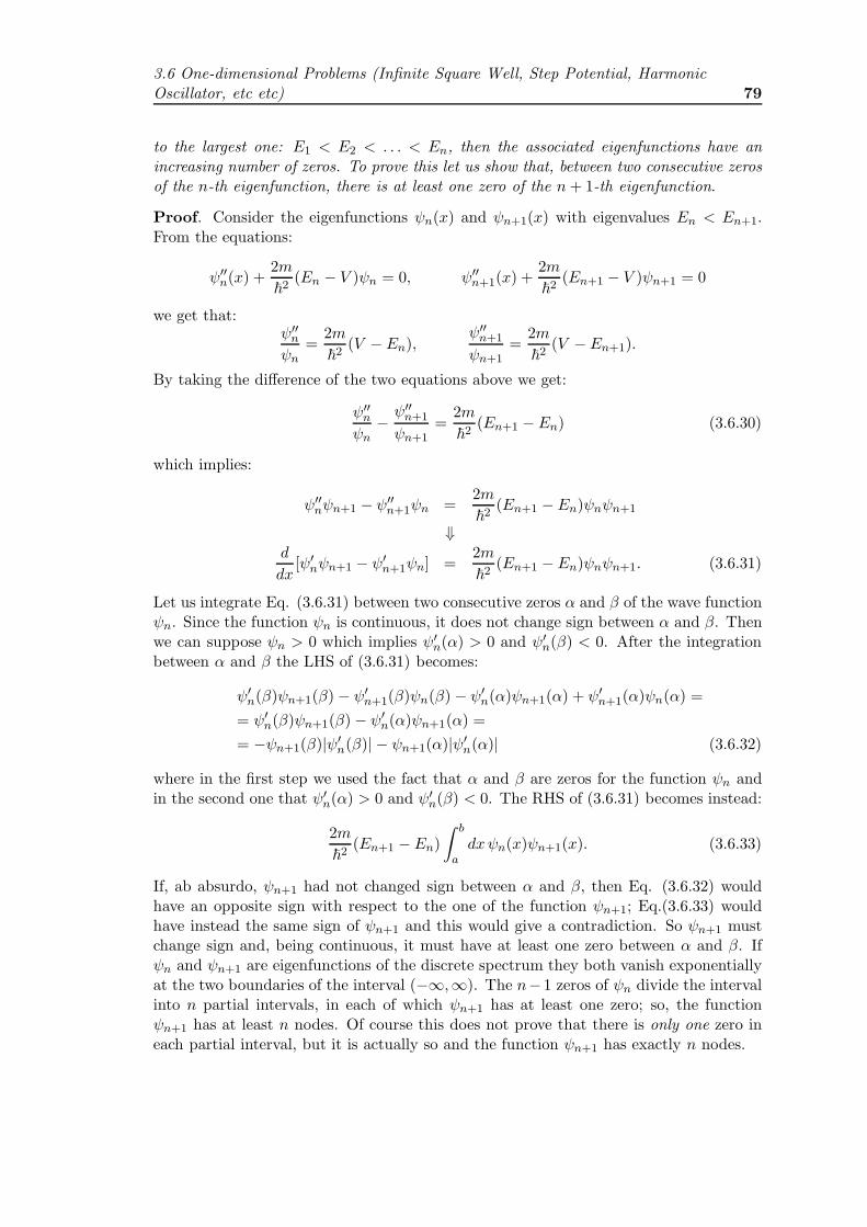
3.6 One-dimensional Problems (Infinite Square Well, Step Potential, HarmonicOscillator, etc etc) 79
to the largest one: E1 < E2 < . . . < En, then the associated eigenfunctions have anincreasing number of zeros. To prove this let us show that, between two consecutive zerosof the n-th eigenfunction, there is at least one zero of the n+ 1-th eigenfunction.
Proof. Consider the eigenfunctions ψn(x) and ψn+1(x) with eigenvalues En < En+1.From the equations:
ψ′′n(x) +
2m
~2(En − V )ψn = 0, ψ′′
n+1(x) +2m
~2(En+1 − V )ψn+1 = 0
we get that:ψ′′n
ψn=
2m
~2(V − En),
ψ′′n+1
ψn+1=
2m
~2(V − En+1).
By taking the difference of the two equations above we get:
ψ′′n
ψn− ψ′′
n+1
ψn+1=
2m
~2(En+1 − En) (3.6.30)
which implies:
ψ′′nψn+1 − ψ′′
n+1ψn =2m
~2(En+1 − En)ψnψn+1
⇓d
dx[ψ′
nψn+1 − ψ′n+1ψn] =
2m
~2(En+1 − En)ψnψn+1. (3.6.31)
Let us integrate Eq. (3.6.31) between two consecutive zeros α and β of the wave functionψn. Since the function ψn is continuous, it does not change sign between α and β. Thenwe can suppose ψn > 0 which implies ψ′
n(α) > 0 and ψ′n(β) < 0. After the integration
between α and β the LHS of (3.6.31) becomes:
ψ′n(β)ψn+1(β)− ψ′
n+1(β)ψn(β) − ψ′n(α)ψn+1(α) + ψ′
n+1(α)ψn(α) =
= ψ′n(β)ψn+1(β)− ψ′
n(α)ψn+1(α) =
= −ψn+1(β)|ψ′n(β)| − ψn+1(α)|ψ′
n(α)| (3.6.32)
where in the first step we used the fact that α and β are zeros for the function ψn andin the second one that ψ′
n(α) > 0 and ψ′n(β) < 0. The RHS of (3.6.31) becomes instead:
2m
~2(En+1 − En)
∫ b
adxψn(x)ψn+1(x). (3.6.33)
If, ab absurdo, ψn+1 had not changed sign between α and β, then Eq. (3.6.32) wouldhave an opposite sign with respect to the one of the function ψn+1; Eq.(3.6.33) wouldhave instead the same sign of ψn+1 and this would give a contradiction. So ψn+1 mustchange sign and, being continuous, it must have at least one zero between α and β. Ifψn and ψn+1 are eigenfunctions of the discrete spectrum they both vanish exponentiallyat the two boundaries of the interval (−∞,∞). The n−1 zeros of ψn divide the intervalinto n partial intervals, in each of which ψn+1 has at least one zero; so, the functionψn+1 has at least n nodes. Of course this does not prove that there is only one zero ineach partial interval, but it is actually so and the function ψn+1 has exactly n nodes.

80 2. Schrodinger Equation
Fig. 3.8: Symmetric well potential.
Problem 13. Find the energy values for the bound states of a particle in the symmetricwell potential plotted in Fig. 3.8.
Solution. As we have seen in Sec. 2.4 the bound states can exist only in the range−U0 < E < 0. Let us write the eigenvalue equations in the three regions I, II, IIIindicated above:
ψ′′1 (x)−
2m
~2|E|ψ1(x) = 0 for x < −b,
ψ′′2 (x) +
2m
~2(U0 − |E|)ψ2(x) = 0 for |x| < b, (3.6.34)
ψ′′3 (x)−
2m
~2|E|ψ3(x) = 0 for x > b.
Let us use the following compact notation:
α ≡(2m
~2|E|
)1/2
> 0, β ≡(2m
~2(U0 − |E|)
)1/2
> 0. (3.6.35)
In the three regions the wave function will have the form:
ψ(x) =
ψIII(x) = Aeαx +Be−αx x > bψII(x) = C sin βx+D cos βx |x| < bψI(x) = Feαx +Ge−αx x < −b.
(3.6.36)
The wave function of a bound state must tend to zero at ±∞ and so A = G = 0. Notealso that |ψIII |2 = B2e−2αx 6= 0 and |ψI |2 = F 2e2αx 6= 0, i.e. the particle can be foundalso outside the well potential differently than in the classical case where it should movewithin the well in order to have a positive kinetic energy.
Now we must impose that the wave function and its derivative be continuous also atx = ±b, that is:
C sinβb+D cos βb = Be−αb
−C sin βb+D cos βb = Fe−αb
βC cos βb− βD sin βb = −αBe−αb
βC cos βb+ βD sin βb = Fαe−αb.

3.6 One-dimensional Problems (Infinite Square Well, Step Potential, HarmonicOscillator, etc etc) 81
By making suitable combinations of the equations above we get:
2C sin βb = (B − F )e−αb (3.6.37)
2βC cos βb = −α(B − F )e−αb (3.6.38)
2D cos βb = (B + F )e−αb (3.6.39)
2βD sinβb = α(B + F )e−αb. (3.6.40)
If C 6= 0 then B − F 6= 0 and dividing (3.6.38) by (3.6.37) we get:
β cotg βb = −α. (3.6.41)
If D 6= 0 then B + F 6= 0 and dividing (3.6.40) by (3.6.39) we get:
β tg βb = α. (3.6.42)
Homework: exercise 6. Prove that Eqs. (3.6.41) and (3.6.42) cannot be satisfied atthe same time.
So we must distinguish two different set of solutions of Eqs. (3.6.37)-(3.6.40):
C = 0, B = F, β tg βb = α (3.6.43)
D = 0, B = −F, β cotg βb = −α. (3.6.44)
In the first case given by Eq. (3.6.43) the solution within the well is ψ(x) = D cos βx,which is an even function. In the second case given by (3.6.44) the solution is ψ(x) =C sinβx, which is an odd function. The energies are determined by solving the equationsβ tg βb = α, β cotg βb = −α (remember that, according to (3.6.35), α and β depend onthe energy E). The equations can be solved only graphically. Putting ξ = βb and η = αbwe get:
E = − ~2
2mb2η2. (3.6.45)
Let us also notice that from the definition of ξ and η:
η2 + ξ2 =2mb2
~2U0 (3.6.46)
while the equation β tgβb = α becomes:
ξtgξ = η. (3.6.47)
Therefore in the first case we must solve the equations:
ξtg ξ = η, ξ2 + η2 =2mb2
~2U0. (3.6.48)
In the second one we have instead:
−ξcotg ξ = η, ξ2 + η2 =2mb2
~2U0. (3.6.49)

82 2. Schrodinger Equation
Fig. 3.9: Solution of the symmetric square well.
The solutions of (3.6.48) and (3.6.49) are given by the intersections of the circle ξ2 +
η2 =2mb2
~2U0 with the curves η = ξtgξ and η = −ξcotgξ in the region ξ, η > 0. For
example in Fig. 3.9 we plotted the second case in which the intersection is between thecircle and η = −ξcotgξ. It is clear that the number of the bound states increases withthe radius of the circle, i.e. with b2U0. This means that the number of bound states
increases with the depth U0 and the width b of the well. If the radius R =
√2m
~2b2U0
of the circle satisfies Nπ
2< R <
N + 1
2π with N = 0, 1, 2, · · · , then the number of
intersections between the circle and the curves, which gives the number of bound states,is N + 1. In the particular case R < π/2 there is only one bound state.
Problem 14. Which is the parity of the energy eigenfunctions of the discrete spectrumfor a time-independent Schrodinger equation with an even potential V (x) = V (−x)?
Solution. If ψ(x) is a solution of the time-independent Schrodinger equation with energyE: [
− ~2
2m
d2
dx2+ V (x)
]ψ(x) = Eψ(x) (3.6.50)
then it is easy to prove that also ψ(−x) is a solution of the Schrodinger equation withthe same value of energy E. In fact let us replace in (3.6.50) x with −x. What we obtainis: [
− ~2
2m
d2
dx2+ V (−x)
]ψ(−x) = Eψ(−x). (3.6.51)

3.6 One-dimensional Problems (Infinite Square Well, Step Potential, HarmonicOscillator, etc etc) 83
Since the potential is even, we have that V (−x) = V (x), which means that we canrewrite (3.6.51) as: [
− ~2
2m
d2
dx2+ V (x)
]ψ(−x) = Eψ(−x).
This proves that both ψ(x) and ψ(−x) are solutions of the Schrodinger equation associ-ated with the same value of energy.
Now let us suppose the functions ψ(x) and ψ(−x) belong to the discrete spectrum.As we have seen in Problem 11, in this case there cannot be degeneracy. So the twowave functions must be linearly dependent: ψ(x) = C ψ(−x). Changing x → −x, weget ψ(−x) = Cψ(x) which implies ψ(x) = Cψ(−x) = C2ψ(x) ⇒ C = ±1. Therefore:
ψ(x) = ±ψ(−x)
which means that the eigenfunctions are even or odd. In the discrete spectrum of aone-dimensional system the wave function ψn+1 has one zero more than ψn. Since theeven (odd) functions have an even (odd) number of zeros we can conclude that theeigenfunctions of the discrete spectrum of an even potential are alternatively even orodd.
In the continuous spectrum there can be degeneracy and so it is not necessary thatψ(x) = C ψ(−x). This implies that the eigenfunctions can have a non-definite parity.
Problem 15. Study the time-independent Schrodinger equation for the step potential
V =
0 forx < 0V0 > 0 forx > 0
.
Solution. The Schrodinger equation in the region x < 0 is:
− ~2
2m
d2
dx2ψ(x) = Eψ(x) =⇒ d2
dx2ψ +
8π2m
h2Eψ = 0.
In the region x ≥ 0 the equation is instead:
− ~2
2m
d2
dx2ψ(x) + V0ψ(x) = Eψ(x) =⇒ d2
dx2ψ +
8π2m
h2(E − V0)ψ = 0.
If we define k20 ≡8π2m
h2E and k2 =
8π2m
h2(E − V0) then the two Schrodinger equations
can be written as:
d2ψ
dx2+ k20ψ = 0 x < 0
d2ψ
dx2+ k2ψ = 0 x > 0.
The solutions can be written as:ψ1(x) = A exp(ik0x) +B exp(−ik0x) x < 0
ψ2(x) = C exp(ikx) +D exp(−ikx) x > 0.(3.6.52)
The boundary conditions are: ψ1(0) = ψ2(0)
ψ′1(0) = ψ′
2(0)

84 2. Schrodinger Equation
and they give: A+B = C +Dk0(A−B) = k(C −D).
(3.6.53)
Let us consider the two cases:
1) E > V0
2) 0 < E < V0.
In classical mechanics in case 1) the particle slows down over the barrier because itskinetic energy becomes smaller in order to preserve the total energy. In case 2) insteadthe particle cannot go beyond the barrier because otherwise its kinetic energy wouldbecome negative.
Let us now analyze the situation in quantum mechanics and consider a wave which atthe beginning is at x = −∞ and propagates towards greater values of x. In the case 1)we have that both k0 and k are real numbers, so the solution (3.6.52) is given by planewaves everywhere. Since in (3.6.53) we have two equations and four unknown quantities,we can put D = 0. With this choice Eq. (3.6.53) becomes:
A+B = Ck0(A−B) = kC
=⇒ A+B
A−B =k0k. (3.6.54)
Let us notice that we cannot choose also B = 0 because otherwise we would obtaink0k
= 1 which is false since k0 > k. Therefore we can say that, even if we consider a
wave propagating towards greater values of x, for x < 0 we cannot throw away the wavepropagating towards smaller values of x, since B must be different from zero. This meansthat, even if the energy of the particle is greater than the step potential, neverthelessthe particle feels the step and is, at least in part, reflected by it.
In the case 2), 0 < E < V0, k is an imaginary number. In order to avoid a divergenceof ψ2(x) we must put either C = 0 or D = 0. If we put D = 0 and we solve Eq. (3.6.53)we get:
A =k0 + i|k|
k0
C
2, B =
k0 − i|k|k0
C
2. (3.6.55)
Therefore there is a reflected wave but there is also a wave which goes beyond the step,i.e. we cannot put C = 0 because otherwise from (3.6.55) we would have A = 0 butthis is not true because at the beginning we have the initial wave. So C 6= 0 and forx > 0 we get ψ2(x) = C exp(−|k|x). This means that the wave can penetrate the step.Also the reflected wave cannot be thrown away: in fact we cannot choose B = 0 becauseotherwise we would have again that k0 = i|k| which is false.
Homework: exercise 7. Solve the Schrodinger equation for a potential like the oneplotted in Fig. 3.10 and prove that the particles in this case can go from region I toregion III even if they have less energy than the step (tunnel effect).
Transmission and Reflection Coefficients. Let us go back to the step potential.Remember that the probability current J in terms of the wave function ψ is given by:

3.6 One-dimensional Problems (Infinite Square Well, Step Potential, HarmonicOscillator, etc etc) 85
Fig. 3.10: Potential for the Tunnel Effect.
J =h
4πim(ψ∗∂xψ −ψ∂xψ∗). For x < 0 and in the case E > V0 the wave function which
propagates towards greater values of x gives the following probability current:
J+(x < 0) =h
2πmAA∗k0. (3.6.56)
The current associated with the wave function propagating towards smaller values of xis:
J−(x < 0) =h
2πmBB∗k0. (3.6.57)
Combining (3.6.54), (3.6.56) and (3.6.57) it is easy to prove that the reflection coefficient
defined as R ≡ J−(x < 0)
J+(x < 0)turns out to be:
R =BB∗
AA∗ =
(k0 − kk0 + k
)2
. (3.6.58)
For x > 0 the current associated with the wave function ψ2 = Ceikx is:
J+(x > 0) =h
2πmCC∗k. (3.6.59)
The transmission coefficient defined as: T ≡ J+(x > 0)
J+(x < 0)becomes:
T =CC∗
AA∗k
k0=
4kk0(k0 + k)2
. (3.6.60)
From (3.6.58) and (3.6.60) it is easy to prove that R+ T = 1. If instead the energy E issmaller than the step potential V0, we get from (3.6.55) that:
R =BB∗
AA∗ = 1, (3.6.61)
i.e. it seems that the entire wave is reflected. This is not true. In fact, since C 6= 0, ifwe perform a measure, we have a certain probability of finding the particle also in theregion x > 0.

86 2. Schrodinger Equation
Problem 16. Find the spectrum and the wave functions of the time independent
Schrodinger equation for a harmonic oscillator V =1
2kx2.
Solution. The Schrodinger equation is
− ~2
2m
d2ψ
dx2+
1
2kx2ψ(x) = Eψ(x). (3.6.62)
With the following change of variables:
ξ ≡ αx, α =
(mk
~2
)1/4
Eq. (3.6.62) becomes:
d2ψ
dξ2+ (λ− ξ2)ψ = 0 (3.6.63)
where
λ ≡ 2E
~
(m
k
)1/2
=2E
~ωc, with ωc =
(k
m
)1/2
. (3.6.64)
The function ψ(ξ) = ξn exp(−1
2ξ2)is a normalizable solution of Eq. (3.6.63) at least for
ξ → +∞. Let us calculate the derivatives:
dψ
dξ= nξn−1e−ξ2/2 − ξn+1e−ξ2/2
d2ψ
dξ2=
(n(n− 1)ξn−2 − nξn − (n+ 1)ξn + ξn+2
)e−ξ2/2.
(3.6.65)
For ξ → ∞ we get thatd2ψ
dξ2∼ ξn+2e−ξ2/2. In the limit ξ → +∞ we can disregard λ
with respect to ξ2 and Eq. (3.6.63) is satisfied:
d2ψ
dξ2− ξ2ψ ∼ ξn+2e−ξ2/2 − ξ2ξne−ξ2/2 = 0. (3.6.66)
Now we let us try to find a complete (and not only asymptotic) solution of (3.6.63) ofthe form:
ψ(ξ) = H(ξ)e−ξ2/2 (3.6.67)
with H(ξ) polynomial in ξ. If we insert (3.6.67) into (3.6.63) we obtain the followingequation for H(ξ):
H ′′(ξ)− 2ξH ′(ξ) + (λ− 1)H(ξ) = 0. (3.6.68)
Let us make this ansatz for H(ξ):
H(ξ) = ξs[a0 + a1ξ + a2ξ2 + . . .] (3.6.69)

3.6 One-dimensional Problems (Infinite Square Well, Step Potential, HarmonicOscillator, etc etc) 87
with a0 6= 0 and s ≥ 0. If we use (3.6.69) in (3.6.68) and we equate the coefficients ofthe same powers of ξ we get:
s(s− 1)a0 = 0
(s+ 1) s a1 = 0
(s+ 2)(s + 1)a2 − (2s + 1− λ)a0 = 0
(s+ 3)(s + 2)a3 − (2s + 3− λ)a1 = 0 (3.6.70)
· · · · · · · · ·(s+ ν + 2)(s + ν + 1)aν+2 − (2s + 2ν + 1− λ)aν = 0.
Since we have chosen a0 6= 0, we get from the first equation that s = 0 or s = 1. Thesecond equation gives s = 0 or a1 = 0 or both of them. The third equation gives a2 asa function of a0; the fourth equation gives a3 as a function of a1; in general the ν-thequation gives aν+2 as a function of aν . According to what we have seen in Problems11 and 14, the functions ψ(x) cannot be degenerate in the discrete part of the spectrumand, since the potential is even, they will be either even or odd: ψ(x) = ±ψ(−x). Thisimplies that H(ξ) must be either even or odd. From (3.6.69) we get the even or oddH(ξ) by choosing a2ν+1 = 0 and s = 0 or a2ν+1 = 0 and s = 1 respectively.
In (3.6.70) there will be a finite or an infinite number of terms depending on how we
choose s and λ. If the series does not stop, then the ratio of the coefficientsaν+2
aν, for
large ν, goes as:aν+2
aν
−→ν→∞
2s + 2ν + 1− λ(s+ ν + 2)(s + ν + 1)
∼ 2
ν. (3.6.71)
For large values of ν the aν behave just like the coefficients of the series expansion of
ξneξ2
(3.6.72)
with n integer1. This means that the power series (3.6.69) becomes an exponentialwhich, combined with the factor e−ξ2/2 of (3.6.67), gives ξneξ
2/2. Such a function is notnormalizable and so it cannot be a solution for the Schrodinger equation. In order tohave an acceptable solution of the Schrodinger equation the series (3.6.69) must stop.This means that in the last term of (3.6.70) λ must satisfy the equation:
λ = 2s+ 2ν + 1. (3.6.73)
If the previous relation holds then aν+2 = 0 and the series stops. Now if we call n = s+νwe obtain that λ = 2n+ 1. By replacing λ with E, see Eq. (3.6.64), we get
En =
(n+
1
2
)~ωc (3.6.74)
which implies that the spectrum of a harmonic oscillator is discrete. The zero-pointenergy is given by the n = 0 term:
E0 =1
2~ωc. (3.6.75)
1In fact two consecutive terms in the series expansion of (3.6.72) are given by ξn(ξ2)m 1m!
andξn(ξ2)m−1 1
(m−1)!and their ratio goes just as 1/m.

88 2. Schrodinger Equation
Also in this case the zero-point energy is due to the uncertainty principle. In fact theeigenfunction associated with E0 is ψ0(ξ) = Ne−ξ2/2, which means that the particle ischaracterized by a finite uncertainty ∆x in the position. From Heisenberg’s relations theassociated uncertainty in the momentum must be finite ∆p 6= 0.
From Eq. (3.6.68) we get that the equation to solve in order to get the eigenfunctionsof a harmonic oscillator is:
H ′′n − 2ξH ′
n + 2nHn = 0 (3.6.76)
whose solutions are the Hermite polynomials:
H0(ξ) = 1, H1(ξ) = 2ξ, H2(ξ) = 4ξ2 − 2
which satisfy the following recurrence relations:
H ′n = 2nHn+1, Hn+1 = 2ξHn − 2nHn−1.
We want to stress the fact that also in the case of the harmonic oscillator the discretenessof the spectrum comes from the renormalizability requirement of the wave function ψn.
3.7 Problems with potentials involving Dirac Deltas.
A function y = f(x) is a map, e.g. between R and R, between C and C or betweenR and C. A functional is a map between a space of functions f and the space of real orcomplex numbers and it is indicated as y = F [f ]. In other words a functional associates anumber to every function f of its domain. In particular a Dirac delta δ(x−x0) associatesto every function f(x) the number f(x0):
∫ ∞
−∞dx δ(x − x0)f(x) = f(x0). (3.7.1)
So the Dirac delta δ(x − x0) is like a very peaked function, different from zero only forx 6= x0. From the definition itself of the Dirac delta (3.7.1) we get:
∫ ∞
−∞dx δ(x − x0) = 1.
This condition suggests that it is possible to “represent” the Dirac delta distribution likea limit of a suitable sequence of functions. For example, if we choose x0 = 0, we havethat the action of the Dirac delta δ(x)
∫ +∞
−∞dx δ(x)f(x) = f(0) (3.7.2)
is the same as the one achieved by the following limit:
δ(x) ∼ liml→∞
l√πe−l2x2
(3.7.3)
where the limit must be done within the integral. In fact, by performing the followingchange of variables x ≡ lx we get:
l√π
∫ ∞
−∞dx e−l2x2
f(x) =1√π
∫ ∞
−∞dxe−x2
f(x/l).

3.7 Problems with potentials involving Dirac Deltas. 89
If we send l→∞ we obtain:
liml→∞
1√π
∫ ∞
−∞dxe−x2
f(x/l) =1√π
∫ ∞
−∞dx e−x2
f(0) = f(0).
So in the limit l → ∞ the sequence of functionsl√πe−l2x2
is a good approximation of
the Dirac delta distribution. Such a sequence of functions is plotted in Fig. 3.11.
Fig. 3.11: Representation of the Dirac delta.
Other representations of the Dirac delta δ(x) are given by:
1
lπ
sin2 lx
x2,
1
lπ
1
x2 + 1l2
,1
π
sin lx
x.
The Dirac delta δ(x − x0) is the generalization to the continuous case of the Kroneckerdelta δij defined as:
δij =
1 if i = j0 if i 6= j
i, j ∈ 1, 2, · · ·N. (3.7.4)
From the definition itself of Kronecker delta every vector f i can be rewritten as f i =∑
j
δijfj. In fact if “i” is a continuous index then f i becomes a function of x, fx = f(x),
and the sum becomes an integral:
f(x) =
∫dy δxyf
y =
∫dy δ(x − y)f(y) (3.7.5)
which is just the action of the Dirac delta δ(x − y). In order to get some practice withthe Dirac delta distributions we are going to perform some problems on them.
Problem 17. The potential energy of a system is U(x) = U(x)+αδ(x−x0) where U(x)is a bounded function. Which is the behavior of the solution of the Schrodinger equationψ(x) and of its derivative near the point x0?

90 2. Schrodinger Equation
Solution. The equation is
− ~2
2mψ′′ + [U(x) + αδ(x − x0)]ψ = Eψ. (3.7.6)
The wave function must be continuous because of its probabilistic meaning. Let us studythe behavior of the derivative by integrating Eq. (3.7.6) between x0 − ǫ and x0 + ǫ withǫ > 0 and let us send ǫ→ 0:
− ~2
2m
∫ x0+ǫ
x0−ǫdxψ′′ = −
∫ x0+ǫ
x0−ǫdx [U (x) + αδ(x− x0)− E]ψ(x)
⇓
− ~2
2m[ψ′(x0 + ǫ)− ψ′(x0 − ǫ)] = −αψ(x0)−
∫ x0+ǫ
x0−ǫ[U(x)− E]ψ(x). (3.7.7)
If ψ(x) is continuous and U(x) is limited we can use the mean value theorem. In thelimit ǫ→ 0 the integral on the RHS of (3.7.7) is zero, so we get:
limǫ→0− ~
2
2m[ψ′(x0 + ǫ)− ψ′(x0 − ǫ)] = −αψ(x0) (3.7.8)
which means
ψ′(x0 + 0)− ψ′(x0 − 0) =2mα
~2ψ(x0). (3.7.9)
This equation tells us that the derivative is not continuous at the point x0. Rememberwhat we have proved in Problem 12: for potentials with a finite gap the derivative ofthe wave function must be continuous. In this case instead, since the Dirac delta at thepoint x0 implies an infinite gap of the potential in x0, the results of Problem 12 cannothold and the derivative is discontinuous.
Problem 18. Find the energy levels and the wave functions of the discrete spectrum ofa particle in a potential U(x) = −αδ(x) with α > 0.
Solution. The Schrodinger equation
− ~2
2mψ′′ − αδ(x)ψ = Eψ
for x 6= 0 becomes the usual equation of a free particle:
− ~2
2mψ′′ = Eψ. (3.7.10)
In order to have normalizable solutions of (3.7.10) the wave functions must be:
ψ(x) = A exp(−kx) x > 0ψ(x) = B exp(kx) x < 0.
(3.7.11)
For the continuity of the wave function the two coefficients A and B must be equal. Therelation between E and k can be obtained by inserting (3.7.11) into (3.7.10):
− ~2
2mAk2 exp(−kx) = EA exp(−kx) =⇒ E = −~
2k2
2m(3.7.12)

3.7 Problems with potentials involving Dirac Deltas. 91
where k must be determined. Using the results of Problem 17, the gap in the derivativeof the wave function is:
ψ′(x0 + 0)− ψ′(x0 − 0) =−2mα~2
ψ(x0) (3.7.13)
which in our case becomes:
−kA exp(−k · 0)− kA exp(k · 0) = −2mα~2
A ⇒ k =mα
~2. (3.7.14)
This implies that there is only one value of k which corresponds to a solution of ourproblem. The associated energy level is given by:
E = − ~2
2mk2 = − ~
2
2m
m2α2
~4= −mα
2
2~2. (3.7.15)
Homework: exercise 8. Prove that the normalized eigenfunction associated with theenergy level (3.7.15) is: ψ =
√k exp[−k|x|].
Problem 19. Prove that the mean value of a conservative force calculated in an energyeigenstate of the discrete spectrum is zero.
Solution. Since the force is conservative it can be written in terms of a potential U as
F = −dUdx
. The mean value of F is:
F =
∫dxF (x)P (x) =
∫dxF (x)ψ∗
nψn = −∫dxψ∗
n
dU
dxψn =
= −∫ ∞
−∞dx
d
dx(U |ψn|2) +
∫ ∞
−∞dx (ψ∗
nUψ′n + ψ∗′
n Uψn). (3.7.16)
The first integral in (3.7.16) gives −U |ψn|2∣∣∣∣∞
−∞= 0 since the wave function ψn tends to
zero for x→ ±∞. In order to evaluate the second integral of (3.7.16) we must rememberthat ψn is a solution of the time-independent Schrodinger equation:
− ~2
2m
∂2ψn
∂x2+ Uψn = Enψn, − ~
2
2m
∂2ψ∗n
∂x2+ Uψ∗
n = Enψ∗n. (3.7.17)
So the second integral of (3.7.16) becomes:
∫ ∞
−∞dx
[(En +
~2
2m
∂2
∂x2
)ψ∗nψ
′n + ψ∗′
n
(En +
~2
2m
∂2
∂x2
)ψn
]=
=~2
2m
∫ ∞
−∞dx
[∂2ψ∗
n
∂x2ψ′n + ψ∗′
n
∂2
∂x2ψn
]+ En
∫ ∞
−∞dx
d
dx(ψ∗
nψn) =
=~2
2m
∫ ∞
−∞dx
d
dx(ψ∗′
n ψ′n) =
~2
2mψ∗′n ψ
′n
∣∣∣∣∞
−∞= 0. (3.7.18)
In the proof above it is crucial that the wave function and its derivative tend to zero at±∞.

92 2. Schrodinger Equation
Homework: exercise 9. Prove that it is not true that the mean value of the force iszero if the wave function is not an energy eigenstate.
Problem 20. Find the energy values for which a particle does not reflect on the followingpotential barrier: U(x) = α[δ(x) + δ(x− a)].
Solution. Let us suppose the particle moves from left to right. If we want to avoidreflection, the wave function must have the form:
ψk(x) =
exp ikx x < 0A sin kx+B cos kx 0 < x < aC exp[ik(x− a)] x > a.
(3.7.19)
In the sector x < 0 we do not have the reflected part R exp−ikx. In the sector x > a, forsymmetry, we must have only the transmitted wave because if we had a wave propagatingtowards smaller values of x, we would have such a kind of wave also for x < 0. Now wecan impose the boundary conditions on the wave function and on its derivative both inx = 0 and in x = a. We can use the results already obtained in the case of Dirac deltapotentials; the wave function will be continuous while the derivative will have a finitegap:
ψ′(x0 + 0)− ψ′(x0 − 0) =2mα
~2ψx0
ψ(x0 + 0) = ψ(x0 − 0).(3.7.20)
Imposing (3.7.20) both on x0 and xa we get
B = 1 (3.7.21)
kA− ik = 2mα/~2 (3.7.22)
A sin ka+B cos ka = C (3.7.23)
ikC − kA cos ka+ kB sin ka = 2mαC/~2. (3.7.24)
We have four equations and A,B,C, k as unknown variables. From (3.7.22) we get
kA = ik + 2mα/~2 ⇒ A = i+ 2mα/k~2. (3.7.25)
Using (3.7.23) and (3.7.25), Eq. (3.7.22) gives:
C =
(i+
2mα
k~2
)sin ka+ cos ka
while (3.7.24) becomes:
ik
[(i+
2mα
k~2
)sin ka+ cos ka
]− k
(i+
2mα
k~2
)cos ka+ k sin ka =
=2mα
~2
[(i+
2mα
k~2
)sin ka+ cos ka
]
which implies:
tg ka = −k ~2
αm. (3.7.26)

3.8 Multidimensional Problems and Separation of Variables 93
Eq. (3.7.26) can be solved graphically by looking for the intersections of the line
y = −k~2
αmwith the curve y = tg ka; the points of intersection give the values of k
and, consequently, of the energies E =~2k2
2mfor which there is no reflection.
3.8 Multidimensional Problems and Separation of Vari-
ables
In order to solve multidimensional problems in quantum mechanics we can use the socalled separation of variables techniques. This method can be applied when the potentialis separable. In Cartesian coordinates the separability of the potential means:
V (x, y, z) = V1(x) + V2(y) + V3(z)
which implies that the Schrodinger equation has the form:
[− ~
2
2m
(∂2
∂x2+
∂2
∂y2+
∂2
∂z2
)+ V1(x) + V2(y) + V3(z)
]ψ(x, y, z) = Eψ(x, y, z).
If we look for solutions of the following type:
ψ(x, y, z) ≡ ψ1(x)ψ2(y)ψ3(z)
the Schrodinger equation becomes:
− ~2
2m
∂2ψ1(x)
∂x2ψ2(y)ψ3(z) + V1(x)ψ1(x)ψ2(y)ψ3(z) +
− ~2
2m
∂2ψ2(y)
∂y2ψ1(x)ψ3(z) + V2(y)ψ1(x)ψ2(y)ψ3(z) + (3.8.1)
− ~2
2m
∂2ψ3(z)
∂z2ψ1(x)ψ2(y) + V3(z)ψ1(x)ψ2(y)ψ3(z) =
= Eψ1(x)ψ2(y)ψ3(z).
By dividing the RHS and the LHS of (3.8.1) by ψ1(x)ψ2(y)ψ3(z) we get:
[− ~
2
2m
∂2ψ1(x)
∂x2+ V1(x)ψ1(x)
]1
ψ1(x)+
+
[− ~
2
2m
∂2ψ2(y)
∂y2+ V2(y)ψ2(y)
]1
ψ2(y)+
+
[− ~
2
2m
∂2ψ3(z)
∂z2+ V3(z)ψ3(z)
]1
ψ3(z)= E.

94 2. Schrodinger Equation
Each line in the previous expression on the LHS is a function of a different variable. Inorder to have the sum equal to a constant, every single term must be a constant:
[− ~
2
2m
∂2ψ1(x)
∂x2+ V1(x)ψ1(x)
]1
ψ1(x)= E1
[− ~
2
2m
∂2ψ2(y)
∂y2+ V2(y)ψ2(y)
]1
ψ2(y)= E2
[− ~
2
2m
∂2ψ3(z)
∂z2+ V3(z)ψ3(z)
]1
ψ3(z)= E3
and moreover the following constraint must hold E = E1 + E2 + E3. Solving the initialthree-dimensional eigenvalue equation is then equivalent to solving the following onedimensional equations:
[− ~
2
2m
∂2ψ1(x)
∂x2+ V1(x)ψ1(x)
]= E1ψ1(x)
[− ~
2
2m
∂2ψ2(y)
∂y2+ V2(y)ψ2(y)
]= E2ψ2(y)
[− ~
2
2m
∂2ψ3(z)
∂z2+ V3(z)ψ3(z)
]= E3ψ3(z).
By solving these three equations separately it is possible to get the three eigenvalues E1,E2, E3 and, by adding them, we obtain the total energy E.
We should point out that a potential may be separable in a set of coordinates but notin another one. For example
V (r, θ, ϕ) = r2 + l2 tan θ + s2 sin2 ϕ (3.8.2)
is separable in the polar coordinates but it is not separable in the Cartesian ones. Infact from:
x = r sin θ cosϕy = r sin θ sinϕz = r cos θ
we easily get:
tan θ =sin θ
cos θ=
√1− z2/r2z/r
=
√r2 − z2z
=
√x2 + y2
z,
tanϕ =y
x=⇒ sinϕ√
1− sin2 ϕ=y
x=⇒ sin2 ϕ =
y2
x2 + y2.
By using the previous relations we get that the potential (3.8.2) is not separable in theCartesian variables x, y, z:
V (x, y, z) = x2 + y2 + z2 + l2√x2 + y2
z+ s2
y2
x2 + y2.

3.8 Multidimensional Problems and Separation of Variables 95
Other potentials are separable in more than one set of variables. For example V (x, y, z) =k(x2 + y2 + z2) is separable in the Cartesian coordinates and also in the polar ones:V (r) = kr2.
As we will see in the next problem and in the following sections, the general strategyto solve a multidimensional problem is to find, whenever is possible, a set of variables(polar, cylindrical, parabolic) in which the potential is separable in order to reduce theproblem to a set of three one-dimensional problems.
Problem 38. Find the spectrum and the eigenfunctions for a two-dimensional infinitewell potential of sides a and b:
V (x, y) =
0
+∞in 0 < x < a, 0 < y < botherwise
and discuss the degeneracy of the energy eigenvalues.
Solution. The Schrodinger equation in 0 < x < a and 0 < y < b is given by:
− ~2
2m
(∂2
∂x2+
∂2
∂y2
)ψ(x, y) = Eψ(x, y)
while the boundary conditions for the wave function are:
ψ(0, y) = ψ(a, y) = ψ(x, 0) = ψ(x, b) = 0.
The potential is separable, so we can look for solutions of the form: ψ(x, y) = ψ1(x)ψ2(y).The eigenvalue equations for ψ1(x) and ψ2(y) become:
− ~2
2m
∂2
∂x2ψ1(x) = Exψ1(x), − ~
2
2m
∂2
∂y2ψ2(y) = Eyψ2(y)
with the constraint Ex + Ey = E and the boundary conditions
ψ1(0) = ψ1(a) = 0, ψ2(0) = ψ2(b) = 0.
So we have two infinite wells, one in the x-variable and one in the y-variable. Theeigenfunctions and the eigenvalues are respectively given by:
ψ1,n(x) =
√2
asin
nπx
a
E1,n =~2
2m
(nπ
a
)2n = 1, 2, · · · ,
ψ2,k(y) =
√2
bsin
kπy
b
E2,k =~2
2m
(kπ
b
)2k = 1, 2, · · · .
Therefore the eigenfunctions and the eigenvalues for the two-dimensional infinite wellpotential are the following ones:
ψn,k(x, y) =
√4
absin
nπx
asin
kπy
b, En,k =
~2π2
2m
[n2
a2+k2
b2
].
If the ratio of the length of the two sides a and b is an irrational number, then all theenergy levels are non-degenerate, otherwise the energy spectrum is in general degenerate.

96 2. Schrodinger Equation
For example if the two sides of the well have the same length, b = a, then the energyeigenvalues are:
En,k =~2
2m
π2
a2
(n2 + k2
)
and, just to give an example, the level for which n2 + k2 = 5 is twofold degenerate,since there are two linearly independent eigenfunctions with the same eigenvalue: E1,2 =
E2,1 = 5~2π2
2ma2. The ground state E1,1 instead is always non-degenerate.

Bibliography
[1] L.D. Landau and E.M. Lisfitz, “Course of Theoretical Physics, vol.1: Mechanics”,(London, Pergamon Press).
[2] H. Goldstein, “Classical Mechanics”, (Reading, MA, Addison-Wesley. Pub.Co.1980).
[3] P. Caldirola, R. Cirelli and R. Prosperi, “Introduzione alla Fisica Teorica” (UTET,Torino, 1982).
[4] E. Fermi, “Notes on Quantum Mechanics” (University of Chicago Press, Chicago,1961).
[5] C. Cohen-Tannoudji, B. Diu and F. Laloe, “Quantum Mechanics” (Wiley, NewYork, 1977).
[6] V. I. Kogan and V. M. Galitskij, “Problems in Quantum Mechanics” (EnglewoodCliffs, Prentice-Hall, NJ, 1963).
[7] F. Constantinescu and E. Magyari, Problems in Quantum Mechanics” (PergamonPress, Oxford, 1971).
[8] R. M. Eisberg and R. Resnick, “Quantum physics of atoms, molecules, solids, nuclei,and particles” (Wiley, New York, 1974).
[9] R. P. Feynman and A. R. Hibbs, “Quantum Mechanics and Path Integrals”(McGraw-Hill Book Co., New York, 1965).