INTRODUCTION TO WAVELETS - profesores.elo.utfsm.clprofesores.elo.utfsm.cl › ... › Docs ›...
76
Adapted from CS474/674 – Prof. George Bebis Department of Computer Science & Engineering University of Nevada (UNR) INTRODUCTION TO WAVELETS
Transcript of INTRODUCTION TO WAVELETS - profesores.elo.utfsm.clprofesores.elo.utfsm.cl › ... › Docs ›...

A d a p t e d f ro m C S 4 7 4 / 6 7 4 – P ro f . G e o r g e B e b i s
D e p a r t m e n t o f C o m p u t e r S c i e n c e & E n g i n e e r i n g U n i v e r s i t y o f N e v a d a ( U N R )
INTRODUCTION TO WAVELETS

¡ It gives us the spectrum of the ‘whole time-series’ § Which is OK if the time-series is stationary § But what if its not?
¡ We need a technique that can “march along” a time series and that is capable of: § Analyzing spectral content in different places § Detecting sharp changes in spectral character
CRITICISM OF FOURIER SPECTRUM

¡ Time/Frequency localization depends on window size. ¡ Once you choose a particular window size, it will be
the same for all frequencies. ¡ Many signals require a more flexible approach - vary
the window size to determine more accurately either time or frequency.
SHORT TIME FOURIER TRANSFORM STFT
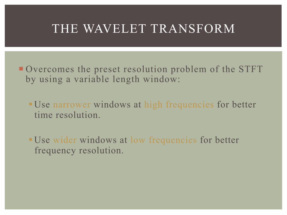
¡ Overcomes the preset resolution problem of the STFT by using a variable length window:
§ Use narrower windows at high frequencies for better
time resolution.
§ Use wider windows at low frequencies for better frequency resolution.
THE WAVELET TRANSFORM

The Wavelet Transform (cont’d)
Wide windows do not provide good localization at high frequencies.

The Wavelet Transform (cont’d)
Use narrower windows at high frequencies.

The Wavelet Transform (cont’d)
Narrow windows do not provide good localization at low frequencies.

The Wavelet Transform (cont’d)
Use wider windows at low frequencies.

The Wavelet Transform (cont’d)
STFT AND DWT BREAKDOWN OF A SIGNAL

WHAT ARE WAVELETS?
¡ Wavelets are functions that “wave” above and below the x-axis, have (1) varying frequency, (2) limited duration, and (3) an average value of zero.
¡ This is in contrast to sinusoids, used by FT, which have infinite energy.
Sinusoid Wavelet

What are Wavelets? (cont’d)
¡ Like sines and cosines in FT, wavelets are used as basis functions ψk(t) in representing other functions f(t):
¡ Span of ψk(t): vector space S containing all functions f(t) that can be represented by ψk(t).
( ) ( )k kk
f t a tψ=∑

What are Wavelets? (cont’d)
¡ There are many different wavelets:
Morlet Haar Daubechies

=ψ jk (t)
What are Wavelets? (cont’d)

What are Wavelets? (cont’d)
time localization
scale/frequency localization
( )/2( ) 2 2 j jjk t t kψ ψ= −
j

MORE ABOUT WAVELETS
change in scale: big s means long
wavelength
normalization
wavelet with scale, s and time, τ
shift in time
Mother wavelet

SHANNON WAVELET
mother wavelet
τ=5, s=2
time
Y(t) = 2 sinc(2t) – sinc(t)

CONTINUOUS WAVELET TRANSFORM (CWT)
( )1( , )t
tC s f t dtssτ
τ ψ ∗ −⎛ ⎞= ⎜ ⎟⎝ ⎠∫
Continuous Wavelet Transform of signal f(t)
translation parameter, measure of time
scale parameter (measure of frequency)
Mother wavelet (window)
normalization constant
Forward CWT:
Scale = 1/j = 1/Frequency

1. Take a wavelet and compare it to a section at the start of the original signal.
2. Calculate a number, C, that represents how closely correlated the wavelet is with this section of the signal. The higher C is, the more the similarity.
CWT: MAIN STEPS

3. Shift the wavelet to the right and repeat steps 1 and 2 until you've covered the whole signal.
CWT: Main Steps (cont’d)

4. Scale the wavelet and repeat steps 1 through 3. 5. Repeat steps 1 through 4 for all scales.
CWT: Main Steps (cont’d)

COEFFICIENTS OF CTW TRANSFORM
( )1( , )t
tC s f t dtssτ
τ ψ ∗ −⎛ ⎞= ⎜ ⎟⎝ ⎠∫
• Wavelet analysis produces a time-scale view of the input signal or image.

¡ Inverse CWT:
Continuous Wavelet Transform (cont’d)
1( ) ( , ) ( )s
tf t C s d dsss τ
ττ ψ τ
−= ∫ ∫
double integral!

FT VS WT
weighted by F(u)
weighted by C(τ,s)

• Simultaneous localization in time and scale - The location of the wavelet allows to explicitly
represent the location of events in time. - The shape of the wavelet allows to represent
different detail or resolution.
PROPERTIES OF WAVELETS

¡ Sparsity: for functions typically found in practice, many of the coefficients in a wavelet representation are either zero or very small.
¡ Linear-time complexity: many wavelet transformations can be accomplished in O(N) time.
Properties of Wavelets (cont’d)
1( ) ( , ) ( )s
tf t C s d dsss τ
ττ ψ τ
−= ∫ ∫

¡ Adaptability: wavelets can be adapted to represent a wide variety of functions (e.g., functions with discontinuities, functions defined on bounded domains etc.).
§ Well suited to problems involving images, open or closed curves, and surfaces of just about any variety.
§ Can represent functions with discontinuities or corners more efficiently (i.e., some have sharp corners themselves).
Properties of Wavelets (cont’d)

Properties of Wavelets (cont’d)
• Admissibility condition:
Implies that Ψ(ω)→0 both as ω→0 and ω→∞, so Ψ(ω) must be band-limited

Fourier spectrum of Shannon Wavelet
frequency, ω
Spectrum of higher scale wavelets
ω

¡ CWT computes all scales and positions in a given range
¡ DWT scales and positions are only computed in powers of 2 (dyadic scales)
¡ This subset can be shown to have the same accuracy as DWT
¡ Dyadic scales allow for tree decompositions
DISCRETE WAVELET TRANSFORM (DWT)
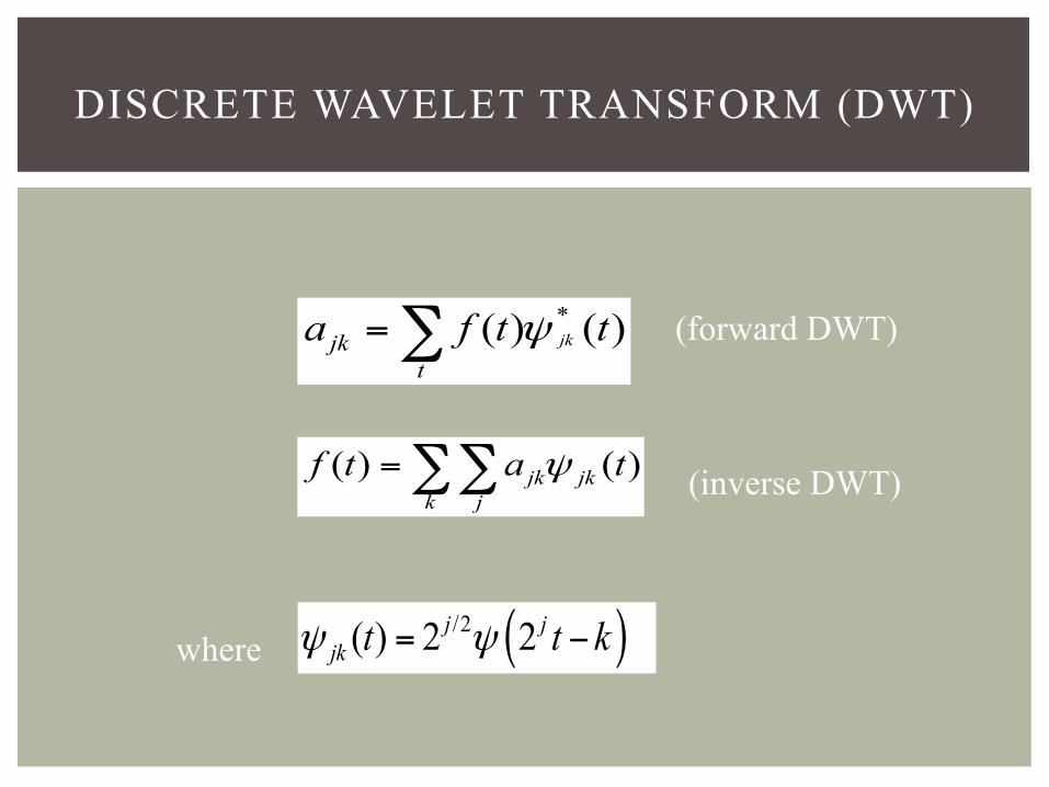
DISCRETE WAVELET TRANSFORM (DWT)
( ) ( )jk jkk j
f t a tψ=∑∑
( )/2( ) 2 2 j jjk t t kψ ψ= −
(inverse DWT)
(forward DWT)
where
*( ) ( )jkjkt
a f t tψ=∑

DFT VS DWT
¡ DFT expansion:
¡ DWT expansion
or
one parameter basis
( ) ( )l ll
f t a tψ=∑
( ) ( )jk jkk j
f t a tψ=∑∑
two parameter basis

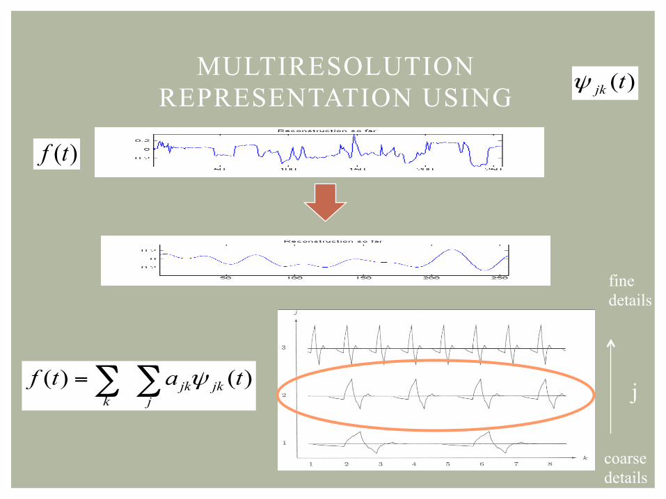
MULTIRESOLUTION REPRESENTATION USING
( ) ( )jk jkk j
f t a tψ=∑ ∑
( )f t
( )jk tψ
j
fine details
coarse details
wider, large translations
MULTIRESOLUTION REPRESENTATION USING
( ) ( )jk jkk j
f t a tψ=∑ ∑
( )f t
( )jk tψ
j
fine details
coarse details

( ) ( )jk jkk j
f t a tψ=∑ ∑
( )f t
j
fine details
coarse details
narrower, small translations
MULTIRESOLUTION REPRESENTATION USING
( )jk tψ

high resolution (more details)
low resolution (less details)
…
( ) ( )jk jkk j
f t a tψ=∑ ∑
( )f t
1̂( )f t
2̂ ( )f t
ˆ ( )sf t
j
MULTIRESOLUTION REPRESENTATION USING
( )jk tψ

Mallat* Filter Scheme
n Mallat was the first to implement this scheme, using a well known filter design called “two channel sub band coder”, yielding a ‘Fast Wavelet Transform’

Approximations and Details:
n Approximations: High-scale, low-frequency components of the signal
n Details: low-scale, high-frequency components
Input Signal
LPF
HPF

Decimation
n The former process produces twice the data it began with: N input samples produce N approximations coefficients and N detail coefficients.
n To correct this, we Down sample (or: Decimate) the filter output by two, by simply throwing away every second coefficient.

Decimation (cont’d)
Input Signal
LPF
HPF
A*
D*
So, a complete one stage block looks like:

Multi-level Decomposition
n Iterating the decomposition process, breaks the input signal into many lower-resolution components: Wavelet decomposition tree:

Wavelet reconstruction
n Reconstruction (or synthesis) is the process in which we assemble all components back
Up sampling (or interpolation) is done by zero inserting between every two coefficients

- Choosing the correct filter is most important. - The choice of the filter determines the shape of the wavelet we use to perform the analysis.
WAVELETS LIKE FILTERS
Relationship of Filters to Wavelet Shape

FILTER BANK REPRESENTATION OF THE DWT DILATIONS

WAVELET PACKET ANALYSIS (DWPA) TREE DECOMPOSITION

Prediction Residual Pyramid
• In the absence of quantization errors, the approximation pyramid can be reconstructed from the prediction residual pyramid. • Prediction residual pyramid can be represented more efficiently.
(with sub-sampling)

Efficient Representation Using “Details”
details D2
L0
details D3
details D1
(no sub-sampling)

Efficient Representation Using Details (cont’d)
representation: L0 D1 D2 D3
A wavelet representation of a function consists of (1) a coarse overall approximation (2) detail coefficients that influence the function at various scales.
(decomposition or analysis) in general: L0 D1 D2 D3…DJ

RECONSTRUCTION (SYNTHESIS) H3=L2+D3
details D2
L0
details D3
H2=L1+D2
H1=L0+D1
details D1
(no sub-sampling)

EXAMPLE - HAAR WAVELETS
¡ Suppose we are given a 1D "image" with a resolution of 4 pixels:
[9 7 3 5]
¡ The Haar wavelet transform is the following:
L0 D1 D2 D3 (with sub-sampling)

Example - Haar Wavelets (cont’d)
¡ Start by averaging the pixels together (pairwise) to get a new lower resolution image:
¡ To recover the original four pixels from the two averaged
pixels, store some detail coefficients.
1

Example - Haar Wavelets (cont’d)
¡ Repeating this process on the averages gives the full decomposition:
1

Example - Haar Wavelets (cont’d)
¡ The Harr decomposition of the original four-pixel image is: ¡ We can reconstruct the original image to a resolution by
adding or subtracting the detail coefficients from the lower-resolution versions.
2 1 -1

Example - Haar Wavelets (cont’d)
Note small magnitude detail coefficients!
Dj
Dj-1
D1 L0
How to compute Di ?

¡ If a set of functions can be represented by a weighted sum of ψ(2jt - k), then a larger set, including the original, can be
represented by a weighted sum of ψ(2j+1t - k):
MULTIRESOLUTION CONDITIONS
time localization
scale/frequency localization
low resolution
high resolution
j

¡ If a set of functions can be represented by a weighted sum of ψ(2jt - k), then a larger set, including the original, can be
represented by a weighted sum of ψ(2j+1t - k):
Multiresolution Conditions (cont’d)
Vj: span of ψ(2jt - k): ( ) ( )j k jkk
f t a tψ=∑
Vj+1: span of ψ(2j+1t - k): 1 ( 1)( ) ( )j k j kk
f t b tψ+ +=∑
1j jV V +⊆

The factor of two scaling means that the spectra of the wavelets divide up the frequency scale into octaves (frequency doubling intervals)
ωny
ω
½ωny ¼ωny 1/8ωny

Ψ1 is the wavelet, now viewed as a bandpass filter.
This suggests a recursion. Replace:
ωny
ω
½ωny ¼ωny 1/8ωny
ωny
ω
½ωny
with
low-pass filter

And then repeat the processes, recursively …

CHOOSING THE LOW-PASS FILTER
The low-pass filter, flp(w) must match wavelet filter, Ψ(ω). A reasonable requirement is:
|flp(ω)|2 + |Ψ(ω)|2 = 1
That is, the spectra of the two filters add up to unity. A pair of such filters are called Quadature Mirror Filters. They are known to have filter coefficients that satisfy the
relationship: ΨN-1-k = (-1)k flp
k Furthermore, it’s known that these filters allows perfect
reconstruction of a time-series by summing its low-pass and high-pass versions

Recursion for wavelet coefficients
γ(s1,t): N/2 coefficients
γ(s2,t): N/4 coefficients
γ(s2,t): N/8 coefficients
Total: N coefficients
time-series of length N
HP LP
↓2 ↓2
HP LP
↓2 ↓2
HP LP
↓2 ↓2
…
γ(s1,t)
γ(s2,t)
γ(s3,t)

Coiflet low pass filter
Coiflet high-pass filter time, t
time, t
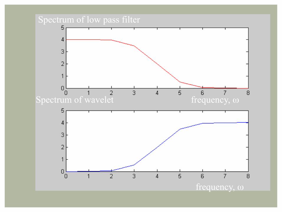
Spectrum of low pass filter
frequency, ω Spectrum of wavelet
frequency, ω

¡ Wavelet decompositions involve a pair of waveforms (mother wavelets):
¡ The two shapes are translated and scaled to produce wavelets (wavelet basis) at different locations and on different scales.
SUMMARY: WAVELET EXPANSION
φ(t) ψ(t)
φ(t-k) ψ(2jt-k)
encode low resolution info
encode details or high resolution info

¡ f(t) is written as a linear combination of φ(t-k) and ψ(2jt-k) :
Summary: wavelet expansion (cont’d)
No se puede mostrar la imagen. Puede que su equipo no tenga suficiente memoria para abrir la imagen o que ésta esté dañada. Reinicie el equipo y, a continuación, abra el archivo de nuevo. Si sigue apareciendo la x roja, puede que tenga que borrar la imagen e insertarla de nuevo.
scaling function wavelet function

¡ Haar scaling and wavelet functions:
1D HAAR WAVELETS
computes average computes details
φ(t) ψ(t)

¡ V j represents all the 2j-pixel images ¡ Functions having constant pieces over 2 j equal-sized
intervals on [0,1).
¡ Note that
1D Haar Wavelets (cont’d)
Examples:
No se puede mostrar la imagen. Puede que su equipo no tenga suficiente memoria para abrir la imagen o que ésta esté dañada. Reinicie el equipo y, a continuación, abra el archivo de nuevo. Si sigue apareciendo la x roja, puede que tenga que borrar la imagen e insertarla de nuevo.
width: 1/2j
ϵ Vj ϵ Vj
No se puede mostrar la imagen. Puede que su equipo no tenga suficiente memoria para abrir la imagen o que ésta esté dañada. Reinicie el equipo y, a continuación, abra el archivo de nuevo. Si sigue apareciendo la x roja, puede que tenga que borrar la imagen e insertarla de nuevo.

1D Haar Wavelets (cont’d)
V0, V1, ..., V j are nested
i.e.,
VJ … V2 V1 coarse details
fine details
1j jV V +⊂

1D Haar Wavelets (cont’d)

EXAMPLE

Example (cont’d)

2D HAAR BASIS FOR STANDARD DECOMPOSITION
To construct the standard 2D Haar wavelet basis, consider all possible outer products of 1D basis functions.
φ0,0(x)
ψ0,0(x)
ψ0,1(x)
ψ1,1(x)
V2=V0+W0+W1
Example:

2D HAAR BASIS FOR STANDARD DECOMPOSITION
To construct the standard 2D Haar wavelet basis, consider all possible outer products of 1D basis functions.
φ00(x), φ00(x) ψ00(x), φ00(x) ψ01(x), φ00(x)
( ) ( )ji jix xϕ ϕ≡ ( ) ( )j
i jix xψ ψ≡

2D HAAR BASIS OF STANDARD DECOMPOSITION
( ) ( )ji jix xϕ ϕ≡
( ) ( )ji jix xψ ψ≡
V2

¡ Noise filtering ¡ Image compression ¡ Fingerprint compression ¡ Image fusion ¡ Recognition ¡ Image matching and retrieval
WAVELETS APPLICATIONS


Original Image Compressed Image
Threshold: 3.5 Zeros: 42% Retained energy: 99.95%