Introduction to the Maximum LikelihoodEstimation Technique

September 24, 2015

So far our Dependent Variable is Continuous

That is, our outcome variable Y is assumed to follow a normaldistribution having mean xb with variance/covariance σ2I. Manyeconomic phenomena do not necessarily fit this storyExamples:

I Foreign Aid Allocation: Many countries receive aid money andmany do not.

I Labor Supply: In your homework, over 1/3 of your sampleworked zero hours

I Unemployment claims: The duration of time on theunemployment roles is left skewed and not normal

I Bankruptcy: examining household bankruptcies revealshouseholds are in 1 or 2 categories: bankrupt or not

I School choice: Students pick one of many schools

An important difference here, is that we can’t use the model errorsas we have so far in the class.

So far our Dependent Variable is Continuous

That is, our outcome variable Y is assumed to follow a normaldistribution having mean xb with variance/covariance σ2I. Manyeconomic phenomena do not necessarily fit this storyExamples:

I Foreign Aid Allocation: Many countries receive aid money andmany do not.

I Labor Supply: In your homework, over 1/3 of your sampleworked zero hours

I Unemployment claims: The duration of time on theunemployment roles is left skewed and not normal

I Bankruptcy: examining household bankruptcies revealshouseholds are in 1 or 2 categories: bankrupt or not

I School choice: Students pick one of many schools

An important difference here, is that we can’t use the model errorsas we have so far in the class.

A focus on the Job Choice Example from MrozSuppose you estimate the model on the full sample and calculateY = xb. Compare to Y

Figure: Actual Working Hours (Y)

Figure: Predicted Working Hours (Y)

Censoring, Truncation, and Sample Selection

The preceding example comes from problems arising fromcensoring/truncation. In effect part of our dependent variable iscontinous, but a large portion of our sample is stacked on aparticular value (e.g. ‘0’ in our example)

I We don’t observe the dependent variable if the individual fallsbelow (or above) a threshold level (truncation)Example: We only observe profits if they are positive.Otherwise, they were negative or zero.

I We don’t observe a lower (or upper) threshold value for thedependent variable if the “true” dependent variable is below acritical value (censoring)Example:The lowest grade level I can assign is an “F”.Different students may have different capabilities (albeit notgood), but all receive an “F”.

For these kinds of problems, use the Tobit or Heckman models.

Dichotomous Choice

Consider a model of the unemployed. Some look for work andsome may not. In this case the dependent variable is binary(1=Looking for work, 0=not looking for work).In this case, we model the probability that an individual i is lookingfor work as

Prob(i ∈ looking) =

∫ ∞−∞

f (xiβ|εi )dεi (1)

Usual assumptions about the error lead to the Probit (based on theNormal Distribution) or the Logit (based on Generalized ExtremeValue Type I).

Multinomial Choice- Choosing among K alternatives

Consider a firm siting decision among K communities. Eachcommunity may offer different tax packages, have differentamenities, etc. The firm’s choice is from among one of the K sites.Now the probability that firm i chooses community k is

Prob(k|i) =∫∞−∞ . . .

∫∞−∞ . . .

∫∞−∞ f (xi1β, . . . , xikβ, . . . , xiKβ|ε)dε

Usual assumptions about the error lead to the multinomial probit(based on the Normal Distribution) or the multinomial logit (basedon Generalized Extreme Value Type I).

Modeling the duration of economic events

Suppose you are interested in the duration of recession i (di ). Theprobability that a recession is less than 1 year long is

Prob(0 < di < 12) =

∫ 12

0f (xib|ε, t)dt (2)

The function f (.) is called the hazard function, and thismethodology was adapted from survival analysis from thebiological literature.

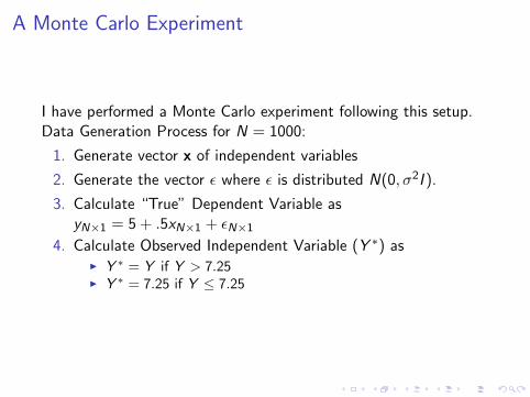
A Monte Carlo Experiment

I have performed a Monte Carlo experiment following this setup.Data Generation Process for N = 1000:

1. Generate vector x of independent variables

2. Generate the vector ε where ε is distributed N(0, σ2I ).

3. Calculate “True” Dependent Variable asyN×1 = 5 + .5xN×1 + εN×1

4. Calculate Observed Independent Variable (Y ∗) asI Y ∗ = Y if Y > 7.25I Y ∗ = 7.25 if Y ≤ 7.25

BIG FAIL for OLS, IV Estimation, and

Traditional Panel Estimators

The Maximum Likelihood Approach

The idea:

I Assume a functional form and distribution for the model errors

I For each observation, construct the probability of observingthe dependent variable yi conditional on model parameters b

I Construct the Log-Likelihood Value

I Search over values for model parameters b that maximizes thesum of the Log-Likelihood Values

MLE: Formal Setup

Consider a sample y =[y1 . . . yi . . . yN

]from the

population. The probability density function (or pdf) of therandom variables yi conditioned on parameters θ is given byf (yi , θ). The joint density of n individually and identicallydistributed observation is

[y1 . . . yi . . . yN

]f (y, θ) =

N∏i=1

f (yi , θ) = L(θ|y) (3)

is often termed the Likelihood Function and the approach istermed Maximum Likelihood Estimation (MLE).

MLE: Our Example

In our excel spreadsheet example,

f (yi , θ) = f (yi , µ|σ2 = 1) =1√

2πσ2e

−(yi−µ)2

2σ2 (4)

It is common practice to work with the Log-Likelihood Function(better numerical properties for computing):

ln(L(θ|y)) =N∑i=1

ln

(1√

2πσ2e

−(yi−µ)2

2σ2

)(5)

We showed how changing the values of µ, allowed us to find themaximum log-likelihood value for the mean of our randomvariables y. Hence the term maximum likelihood.

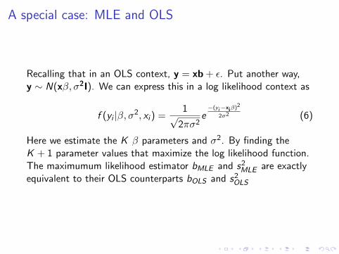
A special case: MLE and OLS

Recalling that in an OLS context, y = xb + ε. Put another way,y ∼ N(xβ, σ2I). We can express this in a log likelihood context as

f (yi |β, σ2, xi ) =1√

2πσ2e

−(yi−xiβ)2

2σ2 (6)

Here we estimate the K β parameters and σ2. By finding theK + 1 parameter values that maximize the log likelihood function.The maximumum likelihood estimator bMLE and s2MLE are exactlyequivalent to their OLS counterparts bOLS and s2OLS

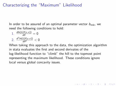
Characterizing the “Maximum” Likelihood

In order to be assured of an optimal parameter vector bmle , weneed the following conditions to hold:

1. dln(L(θ|y ,x))dθ = 0

2. d2ln(L(θ|y ,x))dθ2

< 0

When taking this approach to the data, the optimization algorithmin stata evaluates the first and second derivates of thelog-likelihood function to “climb” the hill to the topmost pointrepresenting the maximum likelihood. These conditions ignorelocal versus global concavity issues.

Properties of MLE

The Maximum Likelihood Estimator has the following properties

I Consistency: plim(θ) = θ

I Asymptotic Normality: θ ∼ N(θ, I (θ)−1)

I Asymptotic Efficiency: θ is asymptotically efficient andachieves the Rao-Cramer Lower Bound for consistentestimators (minimum variance estimator).

I Invariance: The MLE of δ = c(θ) is c(θ) if c(θ) is acontinuous differentiable function.

These properties are roughly analogous to the BLUE properties ofOLS. The importance of asymptotics looms large.

Hypothesis Testing in MLE: The Information Matrix

The variance/covariance matrix of the parameters θ in an MLEframework depend on

I (θ) = −1× ∂2lnL(θ)

∂θ∂θ′(7)

and can be estimated by using our estimated parameter vector θ:

I (θ) = −1× ∂2lnL(θ)

∂θ∂θ′(8)

The inverse of this matrix is our estimated variance covariancematrix for the parameters with standard errors for parameter i

equal to s.e.(i) =√I (θii )−1

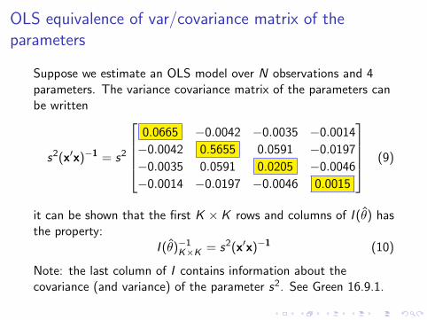
OLS equivalence of var/covariance matrix of theparameters

Suppose we estimate an OLS model over N observations and 4parameters. The variance covariance matrix of the parameters canbe written

s2(x′x)−1 = s2

0.0665 −0.0042 −0.0035 −0.0014

−0.0042 0.5655 0.0591 −0.0197

−0.0035 0.0591 0.0205 −0.0046

−0.0014 −0.0197 −0.0046 0.0015

(9)

it can be shown that the first K × K rows and columns of I (θ) hasthe property:

I (θ)−1K×K = s2(x′x)−1 (10)

Note: the last column of I contains information about thecovariance (and variance) of the parameter s2. See Green 16.9.1.

Nested Hypothesis Testing

Consider a restriction of the form c(θ) = 0. A common restrictionwe consider is

H0 : c(θ) = θ1 = θ2 = . . . = θk = 0 (11)

In an OLS framework, we can use F tests based off of the Model,Total, and Error sum of squares. We don’t have that in the MLEframework because we don’t estimate model errors. Instead, weuse one of three tests available in an MLE setting:

I Likelihood Ratio Test- Examine changes in the joint likelihoodwhen restrictions imposed.

I Wald Test- Look at differences across θ and θr and see if theycan be attributed to sampling error.

I Lagrange Multiplier Test- examine first derivative whenrestrictions imposed.

These are all asymptotically equivalent and all are NESTED tests.

The Likelihood Ratio Test (LR Test)

Denote θu as the unconstrained value of θ estimated via MLE andlet θr be the constrained maximum likelihood estimator. If Lu andLr are the likelihood function values from these parameter vectors(not Log Likelihood Values), the likelihood ratio is then

λ =Lr

Lu(12)

The test statistic, LR = −2× ln(λ), is distributed as χ2(r) degreesof freedom where r are the number of restrictions. In terms oflog-likelihood values, the likelihood ratio test statistic is also

LR = −2 ∗ (ln(Lr )− ln(Lu)) (13)

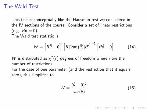
The Wald Test

This test is conceptually like the Hausman test we considered inthe IV sections of the course. Consider a set of linear restrictions(e.g. Rθ = 0).The Wald test statistic is

W =[R θ − 0

]′ [R[Var .(θ)]R ′

]−1 [R θ − 0

](14)

W is distributed as χ2(r) degrees of freedom where r are thenumber of restrictions.For the case of one parameter (and the restriction that it equalszero), this simplifies to

W =(θ − 0)2

var(θ)(15)

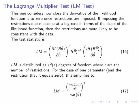
The Lagrange Multiplier Test (LM Test)This one considers how close the derivative of the likelihoodfunction is to zero once restrictions are imposed. If imposing therestrictions doesn’t come at a big cost in terms of the slope of thelikelihood function, then the restrictions are more likely to beconsistent with the data.The test statistic is

LM =

(∂L(R θ)

∂θ

)′I (θ)−1

(∂L(R θ)

∂θ

)(16)

LM is distributed as χ2(r) degrees of freedom where r are thenumber of restrictions. For the case of one parameter (and therestriction that it equals zero), this simplifies to

LM =

(∂L(θ=0)

∂θ

)2var(θ)

(17)

Non-Nested Hypothesis Testing

If one wishes to test hypothesis that are not nested, differentprocedures are needed. A common situation is comparing models(e.g. probit versus the logit). These use Information CriteriaApproaches.

Akaike Information Criterion (AIC) :−2ln(L) + 2K

Bayes/Schwarz Information Criterion (BIC) : −2ln(L) + Kln(N)

where K is the number of parameters in the model and N is thenumber of observations. Choosing the model based on the lowestAIC/BIC is akin to choosing the model with best adjusted R2-although it isn’t necessarily based on goodness of fit, it depends onthe model.

Goodness of fit

Recall that model R2 uses the predicted model error. Here, whilewe have errors, we don’t model them directly. Instead, there hasbeen some work related to goodness of fit in maximum likelihoodsettings. McFadden’s Pseudo R2 is calculated as

Psuedo R2 = 1− ln(L(θ))

ln(L(θconstant))(18)

Some authors (Woolridge) argue that these are poor goodness offit measures and one should tailor goodness of fit criteria for thesituation one is facing.