INTRODUCTION TO

Electrodeposition Module

C o n t a c t I n f o r m a t i o nVisit the Contact COMSOL page at www.comsol.com/contact to submit general inquiries, contact

Technical Support, or search for an address and phone number. You can also visit the Worldwide

Sales Offices page at www.comsol.com/contact/offices for address and contact information.

If you need to contact Support, an online request form is located at the COMSOL Access page at

www.comsol.com/support/case. Other useful links include:

• Support Center: www.comsol.com/support

• Product Download: www.comsol.com/product-download

• Product Updates: www.comsol.com/support/updates

• COMSOL Blog: www.comsol.com/blogs

• Discussion Forum: www.comsol.com/community

• Events: www.comsol.com/events

• COMSOL Video Gallery: www.comsol.com/video

• Support Knowledge Base: www.comsol.com/support/knowledgebase

Part number: CM022502

I n t r o d u c t i o n t o t h e E l e c t r o d e p o s i t i o n M o d u l e © 1998–2018 COMSOL

Protected by patents listed on www.comsol.com/patents, and U.S. Patents 7,519,518; 7,596,474; 7,623,991; 8,457,932; 8,954,302; 9,098,106; 9,146,652; 9,323,503; 9,372,673; and 9,454,625. Patents pending.

This Documentation and the Programs described herein are furnished under the COMSOL Software License Agreement (www.comsol.com/comsol-license-agreement) and may be used or copied only under the terms of the license agreement.

COMSOL, the COMSOL logo, COMSOL Multiphysics, COMSOL Desktop, COMSOL Server, and LiveLink are either registered trademarks or trademarks of COMSOL AB. All other trademarks are the property of their respective owners, and COMSOL AB and its subsidiaries and products are not affiliated with, endorsed by, sponsored by, or supported by those trademark owners. For a list of such trademark owners, see www.comsol.com/trademarks.

Version: COMSOL 5.4

Contents

Introduction . . . . . . . . . . . . . . . . . . . . . . . . . . . . . . . . . . . . . . . . . . . 5

The Electrodeposition Module Physics Interfaces . . . . . . . . . . . . . . . 6

Physics Interface Guide by Space Dimension and Study Type . . . 11

Tutorial —Decorative Plating. . . . . . . . . . . . . . . . . . . . . . . . . . . . 14

Model Definition . . . . . . . . . . . . . . . . . . . . . . . . . . . . . . . . . . . . . . . . . 14

Results . . . . . . . . . . . . . . . . . . . . . . . . . . . . . . . . . . . . . . . . . . . . . . . . . 16

Tutorial — Copper Deposition in a Trench. . . . . . . . . . . . . . . . 29

Model Definition . . . . . . . . . . . . . . . . . . . . . . . . . . . . . . . . . . . . . . . . . 29

Results and Discussion . . . . . . . . . . . . . . . . . . . . . . . . . . . . . . . . . . . . 32

Reference. . . . . . . . . . . . . . . . . . . . . . . . . . . . . . . . . . . . . . . . . . . . . . . 34

| 3

4 |

Introduction

Modeling and simulations are cost-effective ways to understand, optimize, and control electrodeposition processes. The Electrodeposition Module is intended to investigate the influence of different parameters in an electrodeposition cell or on the thickness and composition of deposited layers. Important parameters that can be studied with the module include the following:• Cell geometry• Electrolyte composition and mixing• Electrode kinetics• Operating potential and average current density• Temperature

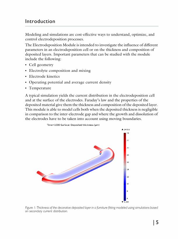
A typical simulation yields the current distribution in the electrodeposition cell and at the surface of the electrodes. Faraday’s law and the properties of the deposited material give them the thickness and composition of the deposited layer. This module is able to model cells both when the deposited thickness is negligible in comparison to the inter-electrode gap and where the growth and dissolution of the electrodes have to be taken into account using moving boundaries.

Figure 1: Thickness of the decorative deposited layer in a furniture fitting modeled using simulations based on secondary current distribution.

| 5

The targeted applications for the Electrodeposition Module include the following:• Copper deposition for electronics and electrical applications• Metal deposition for protection of parts, such as corrosion protection and

protection against wear• Decoration of metals and plastic parts• Electroforming of parts with thin and complex structure• Metal electrowinning

The next section introduces you to the available physics interfaces for this module and provides a brief overview of their use. It also includes a table listing the physics interfaces by space dimension and preset study type.The rest of the introduction includes two tutorials. The first is a secondary current distribution model (secondary here means that we are including ohmic drops and activation overpotentials, but neglecting mass transport effects) where the thickness of the deposited layer can be neglected in the simulation and it therefore uses a fixed geometry. Go to the Tutorial —Decorative Plating to get started with this example. The second model is a full tertiary current density distribution model (tertiary here means that we include ohmic drops, activation potentials and mass transport) that also accounts for the changes in the shapes of the cathode and anode surfaces using moving boundaries. Go to the Tutorial — Copper Deposition in a Trench to start working with this model.

The Electrodeposition Module Physics InterfacesThe module has a number of physics interfaces, which describe different phenomena in the electrolyte and at the electrodes in electrodeposition cells. A number of examples exemplify the use of these physics interfaces, which are based on the conservation of current, charge, chemical species, and energy. Figure 2

6 |

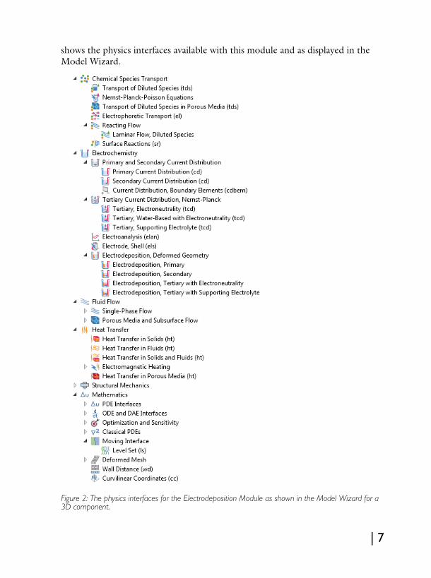
shows the physics interfaces available with this module and as displayed in the Model Wizard.

Figure 2: The physics interfaces for the Electrodeposition Module as shown in the Model Wizard for a 3D component.

| 7

THE CURRENT DISTRIBUTION INTERFACES

The Electrochemistry interfaces include the Primary Current Distribution ( ), Secondary Current Distribution ( ), and Tertiary Current Distribution, Nernst Planck ( ) interfaces. These are generic physics interfaces that can be used to model most kinds of electrochemical cells. These interfaces include functionality to model the current distribution the electrolyte as well as the deposition and thickness evolution of thin layers on the electrode surfaces. However, if the thickness of the deposited layer is of the same order of magnitude (or one order lower) compared to the geometrical details of the electrodes, then the one of the Electrodeposition, Deformed Geometry ( ) interfaces may have to be used instead. These interfaces are described in the next section.The Primary Current Distribution ( ) interface assumes a perfectly mixed electrolyte and neglects the activation losses for the charge transfer reactions. It should only be used for fast kinetics, where the activation losses are substantially smaller than the ohmic losses. The assumption of a perfectly mixed electrolyte implies that the electrolyte conductivity is not affected by the magnitude of the currents.In the Secondary Current Distribution ( ) interface the activation overpotential for the electrochemical reactions is taken into account.The Primary and Secondary Current Distribution interfaces may be combined with a Chemical Species Transport interface (described below) in order to incorporate kinetic effects of active species in the electrolyte or adsorbed species on an electrode surface.The Current Distribution, Boundary Elements ( ) interface can be used for solving primary and secondary current distribution problems on geometries based on edge (beam or wire) and surface elements. The interface uses a boundary element method (BEM) formulation to solve for the charge transfer equation in an electrolyte of constant conductivity, where the electrodes are specified on boundaries or as tubes with a given radius around the edges. You typically use this interface in order to reduce the meshing and solution time for large geometries where a significant part of the geometry can be approximated as tubes along edges.The Tertiary Current Distribution, Nernst-Planck ( ) interface accounts for the transport of species through diffusion, migration, and convection. It is therefore able to describe the effects of variations in domain composition on the electrochemical processes. The kinetic expressions for the electrochemical reactions account for both activation and concentration overpotential.

8 |

THE ELECTRODEPOSITION, DEFORMED GEOMETRY INTERFACES

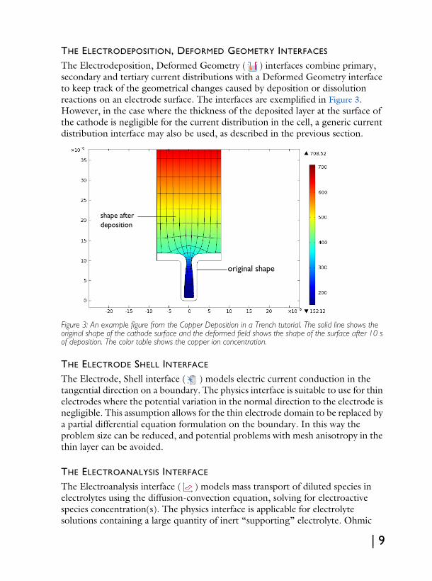
The Electrodeposition, Deformed Geometry ( ) interfaces combine primary, secondary and tertiary current distributions with a Deformed Geometry interface to keep track of the geometrical changes caused by deposition or dissolution reactions on an electrode surface. The interfaces are exemplified in Figure 3. However, in the case where the thickness of the deposited layer at the surface of the cathode is negligible for the current distribution in the cell, a generic current distribution interface may also be used, as described in the previous section.

Figure 3: An example figure from the Copper Deposition in a Trench tutorial. The solid line shows the original shape of the cathode surface and the deformed field shows the shape of the surface after 10 s of deposition. The color table shows the copper ion concentration.

THE ELECTRODE SHELL INTERFACE

The Electrode, Shell interface ( ) models electric current conduction in the tangential direction on a boundary. The physics interface is suitable to use for thin electrodes where the potential variation in the normal direction to the electrode is negligible. This assumption allows for the thin electrode domain to be replaced by a partial differential equation formulation on the boundary. In this way the problem size can be reduced, and potential problems with mesh anisotropy in the thin layer can be avoided.

THE ELECTROANALYSIS INTERFACE

The Electroanalysis interface ( ) models mass transport of diluted species in electrolytes using the diffusion-convection equation, solving for electroactive species concentration(s). The physics interface is applicable for electrolyte solutions containing a large quantity of inert “supporting” electrolyte. Ohmic

original shape

shape after deposition

| 9

losses are assumed to be negligible. The physics interface includes tailor-made functionality for setting up cyclic voltammetry problems.

THE CHEMICAL SPECIES TRANSPORT INTERFACES

The Surface Reactions interface ( ) found in Chemical Species Transport can be set up to model adsorbed species on an electrode surface.The Transport of Diluted Species interface ( ) is available under the Chemical Species Transport Branch. In combination with the Secondary Current Distribution interface ( ), this physics interface can be used to model systems with supporting electrolytes. In these systems, the ions that give the largest contribution to the conduction of current are assumed to be present in uniform concentrations.The Nernst-Planck-Poisson Equations ( ) interface can be used for investigation of charge and ion distributions within the electrochemical double layer where charge neutrality cannot be assumed. A requisite when using this interface is that the double layer, which typically is in the range of tens nanometers, is fully resolved in the mesh.The Transport of Diluted Species in Porous Media interface ( ) is also available and describes species transport between the fluid, solid, and gas phases in saturated and variably saturated porous media. It applies to one or more species that move primarily within a fluid filling (saturated) or partially filling (unsaturated) the voids in a solid porous medium. The pore space not filled with fluid contains an immobile gas phase. Using these, models including a combination of porous media types can be studied.The Electrophoretic Transport ( ) interface can be used to investigate the transport of weak acids, bases, and ampholytes in aqueous solvents. The physics interface is typically used to model various electrophoresis modes, such as zone electrophoresis, isothachophoresis, isoelectric focusing, and moving boundary electrophoresis, but is applicable to any aqueous system involving multiple acid-base equilibria.The Surface Reactions interface ( ) can be used model reactions and translateral transport of surface (adsorbed) species.

OTHER PHYSICS INTERFACES

The Fluid Flow interfaces can be combined with the above interfaces to model free and forced convection in the electrolytic cell.The Heat Transfer interfaces have ready-made formulations for the contribution of Joule heating, and other electrochemical losses, to the thermal balance in the cell.

10 |

The Level Set interface can be used in problems including deforming electrodes, subject to topological changes.The detailed equations and assumptions that are defined by the physics interfaces are formulated in the Electrodeposition Module User’s Guide and the COMSOL Multiphysics Reference Manual.

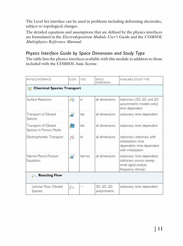
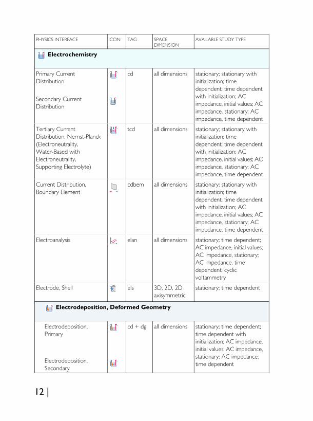
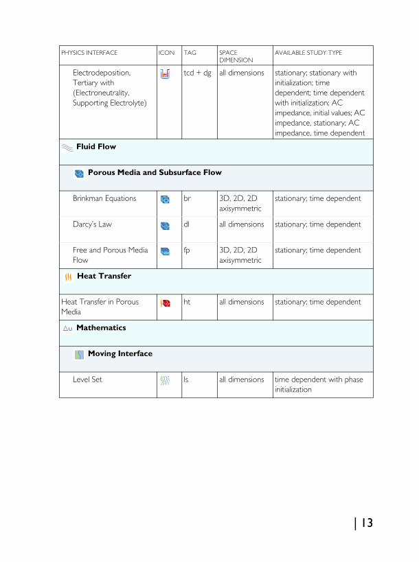
Physics Interface Guide by Space Dimension and Study TypeThe table lists the physics interfaces available with this module in addition to those included with the COMSOL basic license.

PHYSICS INTERFACE ICON TAG SPACE DIMENSION

AVAILABLE STUDY TYPE

Chemical Species Transport

Surface Reactions sr all dimensions stationary (3D, 2D, and 2D axisymmetric models only); time dependent

Transport of Diluted Species

tds all dimensions stationary; time dependent

Transport of Diluted Species in Porous Media

tds all dimensions stationary; time dependent

Electrophoretic Transport el all dimensions stationary; stationary with initialization; time dependent; time dependent with initialization

Nernst-Planck-Poisson Equations

tds+es all dimensions stationary; time dependent; stationary source sweep; small-signal analysis, frequency domain

Reacting Flow

Laminar Flow, Diluted Species

— 3D, 2D, 2D axisymmetric

stationary; time dependent

| 11

Electrochemistry

Primary Current Distribution

Secondary Current Distribution

cd all dimensions stationary; stationary with initialization; time dependent; time dependent with initialization; AC impedance, initial values; AC impedance, stationary; AC impedance, time dependent

Tertiary Current Distribution, Nernst-Planck (Electroneutrality, Water-Based with Electroneutrality, Supporting Electrolyte)

tcd all dimensions stationary; stationary with initialization; time dependent; time dependent with initialization; AC impedance, initial values; AC impedance, stationary; AC impedance, time dependent

Current Distribution, Boundary Element

cdbem all dimensions stationary; stationary with initialization; time dependent; time dependent with initialization; AC impedance, initial values; AC impedance, stationary; AC impedance, time dependent

Electroanalysis elan all dimensions stationary; time dependent; AC impedance, initial values; AC impedance, stationary; AC impedance, time dependent; cyclic voltammetry

Electrode, Shell els 3D, 2D, 2D axisymmetric

stationary; time dependent

Electrodeposition, Deformed Geometry

Electrodeposition, Primary

Electrodeposition, Secondary

cd + dg all dimensions stationary; time dependent; time dependent with initialization; AC impedance, initial values; AC impedance, stationary; AC impedance, time dependent

PHYSICS INTERFACE ICON TAG SPACE DIMENSION

AVAILABLE STUDY TYPE

12 |

Electrodeposition, Tertiary with (Electroneutrality, Supporting Electrolyte)

tcd + dg all dimensions stationary; stationary with initialization; time dependent; time dependent with initialization; AC impedance, initial values; AC impedance, stationary; AC impedance, time dependent

Fluid Flow

Porous Media and Subsurface Flow

Brinkman Equations br 3D, 2D, 2D axisymmetric

stationary; time dependent

Darcy’s Law dl all dimensions stationary; time dependent

Free and Porous Media Flow

fp 3D, 2D, 2D axisymmetric

stationary; time dependent

Heat Transfer

Heat Transfer in Porous Media

ht all dimensions stationary; time dependent

Mathematics

Moving Interface

Level Set ls all dimensions time dependent with phase initialization

PHYSICS INTERFACE ICON TAG SPACE DIMENSION

AVAILABLE STUDY TYPE

| 13

Tutorial —Decorative Plating

This electroplating model uses secondary current distribution with full Butler-Volmer kinetics for the metal deposition or dissolution reaction on the cathode and anode. A competing hydrogen evolution reaction is also present on the cathode. The thickness of the deposited layer at the cathode is computed as well as the current efficiency.

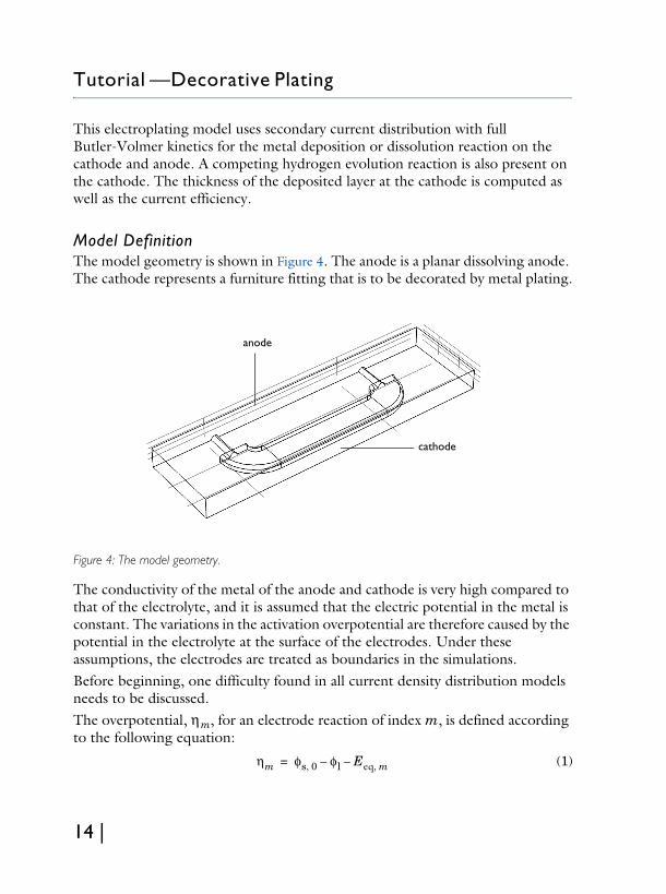
Model DefinitionThe model geometry is shown in Figure 4. The anode is a planar dissolving anode. The cathode represents a furniture fitting that is to be decorated by metal plating.

Figure 4: The model geometry.

The conductivity of the metal of the anode and cathode is very high compared to that of the electrolyte, and it is assumed that the electric potential in the metal is constant. The variations in the activation overpotential are therefore caused by the potential in the electrolyte at the surface of the electrodes. Under these assumptions, the electrodes are treated as boundaries in the simulations.Before beginning, one difficulty found in all current density distribution models needs to be discussed.The overpotential, ηm, for an electrode reaction of index m, is defined according to the following equation:

(1)

anode

cathode

ηm φs 0, φl– Eeq m,–=

14 |

where denotes the electric potential of the metal, denotes the potential in the electrolyte, and Eeq,m denotes the difference between the metal and electrolyte potentials at the electrode surface measured at equilibrium using a common reference potential. The electric potential of one of the electrodes may be bootstrapped, so that all other potentials are measured with this reference (this bootstrap can actually be achieved by fixing the potential at any point in the cell). In this case, the electric potential of the metal is selected at the cathode as a bootstrap by setting this potential to 0 V. This implies that the electric potential of the metal at the anode is equal to the cell voltage. The potential of the electrolyte floats and adapts to satisfy the balance of current, so that an equal amount of current that leaves at the cathode also enters at the anode. This then determines the overpotential at the anode and the cathode.

ELECTROLYTE CHARGE TRANSPORT

Use the Electrodeposition, Secondary interface to solve for the electrolyte potential, φl(V), assuming bulk electroneutrality:

(2)

where il (A/m2) is the electrolyte current density vector and σl (S/m) is the electrolyte conductivity, which is assumed to be a constant. Use the default Insulation condition for all boundaries except the anode and cathode surfaces:

(3)

where n is the normal vector, pointing out of the domain.The main electrode reaction on both the anode and the cathode surfaces is the nickel deposition/dissolution reaction according to

(4)

Using the Butler-Volmer equation to model this reaction will set the local current density to

(5)

The rate of deposition at the cathode boundary surfaces and the rate of dissolution at the anode boundary surface, with a velocity in the normal direction, v (m/s), is calculated according to

φs 0, φl

il σl∇φl–=

∇ i⋅ l 0=

n il⋅ 0=

Ni2+ 2e-+ Ni(s)⇔

iloc Ni, i0 Ni,αaFηNi

RT------------------- αcFηNi

RT-------------------–

exp–exp =

| 15

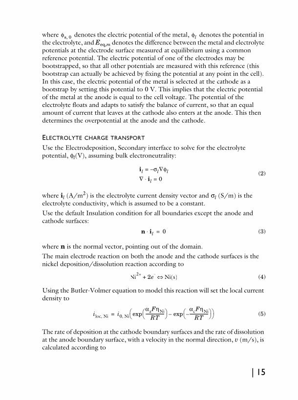
(6)

where M is the mean molar mass (59 g/mol) and ρ is the density (8900 kg/m3) of the nickel atoms and n is number of participating electrons. It should be noted that the local current density is positive at the anode surface and it is negative at the cathode surfaces.On the anode the electrolyte current density is set to the local current density of the nickel deposition reaction:

(7)

On the cathode, add a second electrode reaction to model the parasitic hydrogen evolution reaction:

(8)

Using cathodic Tafel equation to model the kinetics of the hydrogen reaction on the cathode will set the local current density to

(9)

The hydrogen reaction will not contribute to the rate of deposition of nickel, but it will contribute to the total current density at the cathode surface:

(10)

Solve the model in a time-dependent study, simulating the electroplating for 600 s.

ResultsThe figure below shows the thickness of the deposited layer after 600 s of deposition. The variations in thickness are relatively large, more than a factor of 5 between the thinnest and thickest parts. This suggests the need for an improvement of the cell geometry. Another alternative is to add surface active

viloc Ni,

nF---------------M

ρ-----=

n il⋅ iloc Ni,=

2H+ 2e-+ H2⇔

iloc H, i– 0 H, 10ηH Ac⁄–

=

n il⋅ iloc Ni, iloc H,+=

16 |

species, also called levelers, that increase the kinetic losses at the electrode surfaces. These levelers help maintain a uniform current density.

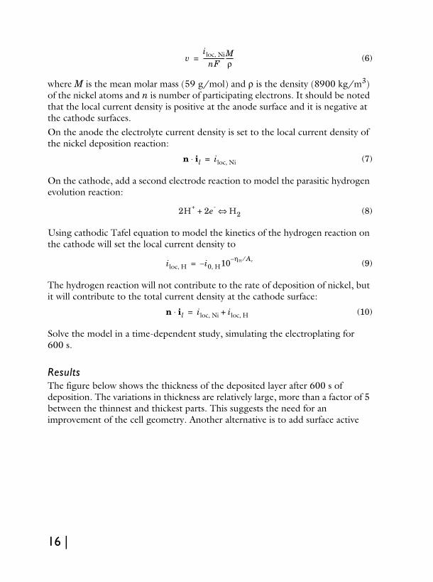
The second figure, shown below, depicts the local current efficiency over the cathode surface. The efficiency is calculated as the nickel deposition current density divided by the total current density at the cathode and is around 97%.

| 17

Model Wizard

Note: These instructions are for the physics interface on Windows but apply, with minor differences, also to Linux and Mac.

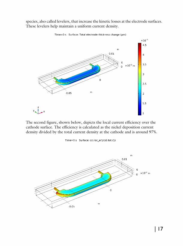
1 To start the software, double-click the COMSOL icon on the desktop. When the software opens, you can choose to use the Model Wizard to create a new COMSOL model or Blank Model to create one manually. For this tutorial, click the Model Wizard button.If COMSOL is already open, you can start the Model Wizard by selecting New from the File menu and then click Model Wizard .

The Model Wizard guides you through the first steps of setting up a model. The next window lets you select the dimension of the modeling space.

2 In the Space Dimension window click the 3D button .3 In the Select Physics tree, select Electrochemistry>Primary and Secondary

Current Distribution, click Secondary Current Distribution (cd) .4 Click Add then click the Study button.5 In the tree under Preset Studies, click Time Dependent with Initialization .6 Click Done .

Global Definit ions

Load the parameter values to be used in the model from a parameter file.

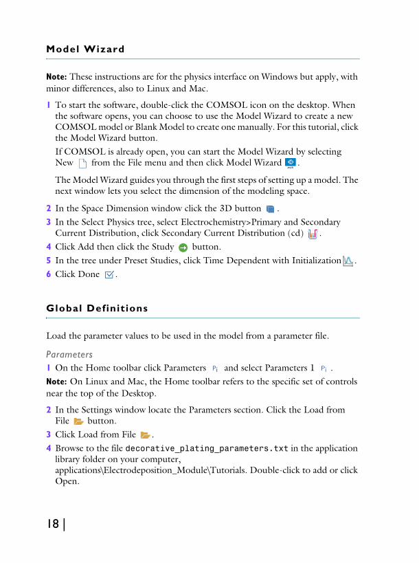
Parameters1 On the Home toolbar click Parameters and select Parameters 1 .Note: On Linux and Mac, the Home toolbar refers to the specific set of controls near the top of the Desktop.

2 In the Settings window locate the Parameters section. Click the Load from File button.

3 Click Load from File . 4 Browse to the file decorative_plating_parameters.txt in the application

library folder on your computer, applications\Electrodeposition_Module\Tutorials. Double-click to add or click Open.

18 |

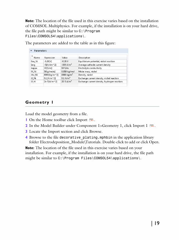
Note: The location of the file used in this exercise varies based on the installation of COMSOL Multiphysics. For example, if the installation is on your hard drive, the file path might be similar to C:\Program Files\COMSOL54\applications\.

The parameters are added to the table as in this figure:

Geometry 1

Load the model geometry from a file.1 On the Home toolbar click Import .2 In the Model Builder under Component 1>Geometry 1, click Import 1 .3 Locate the Import section and click Browse.4 Browse to the file decorative_plating.mphbin in the application library

folder Electrodeposition_Module\Tutorials. Double-click to add or click Open.Note: The location of the file used in this exercise varies based on your installation. For example, if the installation is on your hard drive, the file path might be similar to C:\Program Files\COMSOL54\applications\.

| 19

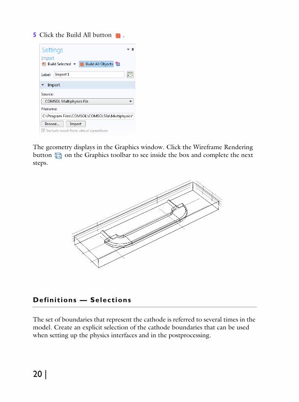
5 Click the Build All button .

The geometry displays in the Graphics window. Click the Wireframe Rendering button on the Graphics toolbar to see inside the box and complete the next steps.

Definit ions — Selections

The set of boundaries that represent the cathode is referred to several times in the model. Create an explicit selection of the cathode boundaries that can be used when setting up the physics interfaces and in the postprocessing.

20 |

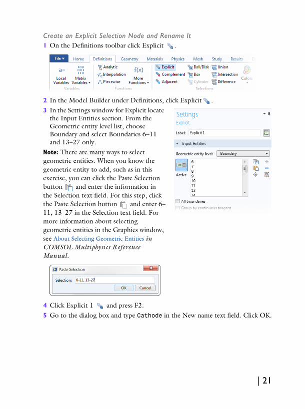
Create an Explicit Selection Node and Rename It1 On the Definitions toolbar click Explicit .

2 In the Model Builder under Definitions, click Explicit .3 In the Settings window for Explicit locate

the Input Entities section. From the Geometric entity level list, choose Boundary and select Boundaries 6–11 and 13–27 only.

Note: There are many ways to select geometric entities. When you know the geometric entity to add, such as in this exercise, you can click the Paste Selection button and enter the information in the Selection text field. For this step, click the Paste Selection button and enter 6–11, 13–27 in the Selection text field. For more information about selecting geometric entities in the Graphics window, see About Selecting Geometric Entities in COMSOL Multiphysics Reference Manual.

4 Click Explicit 1 and press F2.5 Go to the dialog box and type Cathode in the New name text field. Click OK.

| 21

Secondary Current Distribution

Now start setting up the current distribution model, beginning with the settings for the electrolyte.

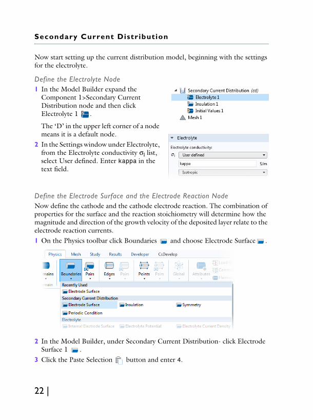
Define the Electrolyte Node1 In the Model Builder expand the

Component 1>Secondary Current Distribution node and then click Electrolyte 1 .

The ‘D’ in the upper left corner of a node means it is a default node.

2 In the Settings window under Electrolyte, from the Electrolyte conductivity σl list, select User defined. Enter kappa in the text field.

Define the Electrode Surface and the Electrode Reaction NodeNow define the cathode and the cathode electrode reaction. The combination of properties for the surface and the reaction stoichiometry will determine how the magnitude and direction of the growth velocity of the deposited layer relate to the electrode reaction currents. 1 On the Physics toolbar click Boundaries and choose Electrode Surface .

2 In the Model Builder, under Secondary Current Distribution- click Electrode Surface 1 .

3 Click the Paste Selection button and enter 4.

22 |

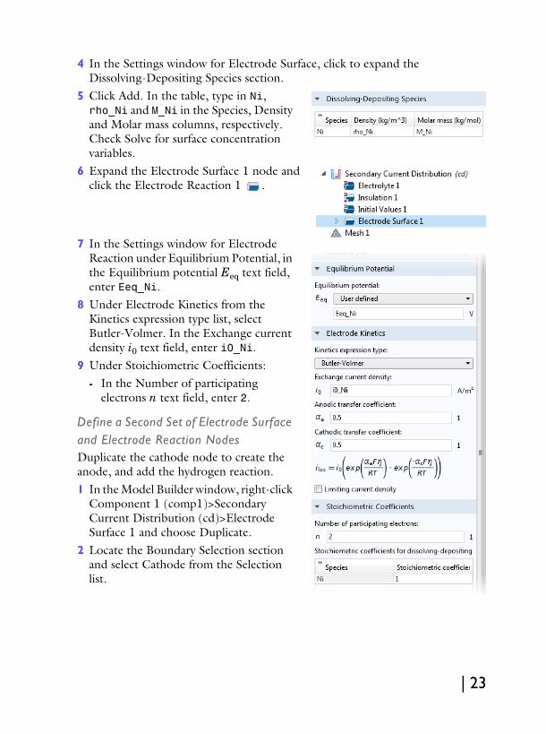
4 In the Settings window for Electrode Surface, click to expand the Dissolving-Depositing Species section.

5 Click Add. In the table, type in Ni, rho_Ni and M_Ni in the Species, Density and Molar mass columns, respectively. Check Solve for surface concentration variables.

6 Expand the Electrode Surface 1 node and click the Electrode Reaction 1 .

7 In the Settings window for Electrode Reaction under Equilibrium Potential, in the Equilibrium potential Eeq text field, enter Eeq_Ni.

8 Under Electrode Kinetics from the Kinetics expression type list, select Butler-Volmer. In the Exchange current density i0 text field, enter i0_Ni.

9 Under Stoichiometric Coefficients:- In the Number of participating

electrons n text field, enter 2.

Define a Second Set of Electrode Surface and Electrode Reaction NodesDuplicate the cathode node to create the anode, and add the hydrogen reaction.1 In the Model Builder window, right-click

Component 1 (comp1)>Secondary Current Distribution (cd)>Electrode Surface 1 and choose Duplicate.

2 Locate the Boundary Selection section and select Cathode from the Selection list.

| 23

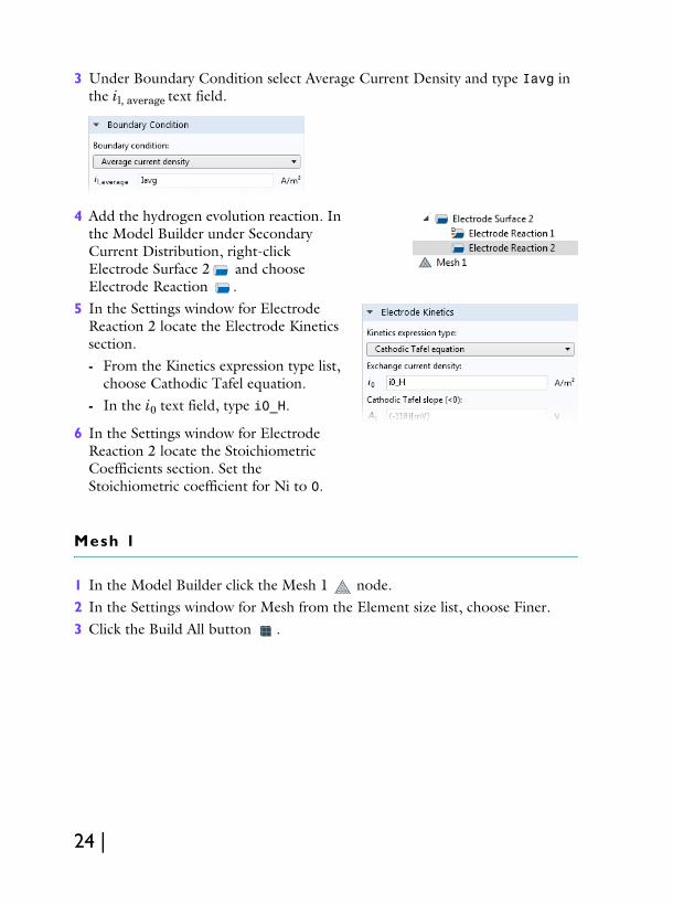
3 Under Boundary Condition select Average Current Density and type Iavg in the il, average text field.

4 Add the hydrogen evolution reaction. In the Model Builder under Secondary Current Distribution, right-click Electrode Surface 2 and choose Electrode Reaction .

5 In the Settings window for Electrode Reaction 2 locate the Electrode Kinetics section. - From the Kinetics expression type list,

choose Cathodic Tafel equation.- In the i0 text field, type i0_H.

6 In the Settings window for Electrode Reaction 2 locate the Stoichiometric Coefficients section. Set the Stoichiometric coefficient for Ni to 0.

Mesh 1

1 In the Model Builder click the Mesh 1 node.2 In the Settings window for Mesh from the Element size list, choose Finer. 3 Click the Build All button .

24 |

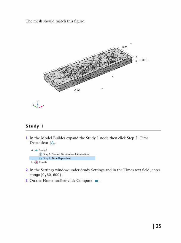
The mesh should match this figure.

Study 1

1 In the Model Builder expand the Study 1 node then click Step 2: Time Dependent .

2 In the Settings window under Study Settings and in the Times text field, enter range(0,60,600).

3 On the Home toolbar click Compute .

| 25

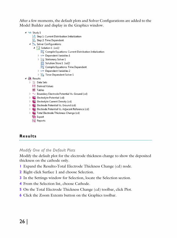
After a few moments, the default plots and Solver Configurations are added to the Model Builder and display in the Graphics window.

Results

Modify One of the Default PlotsModify the default plot for the electrode thickness change to show the deposited thickness on the cathode only.1 Expand the Results>Total Electrode Thickness Change (cd) node.2 Right-click Surface 1 and choose Selection.3 In the Settings window for Selection, locate the Selection section.4 From the Selection list, choose Cathode.5 On the Total Electrode Thickness Change (cd) toolbar, click Plot.6 Click the Zoom Extents button on the Graphics toolbar.

26 |

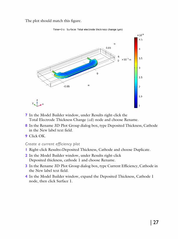
The plot should match this figure.

7 In the Model Builder window, under Results right-click the Total Electrode Thickness Change (cd) node and choose Rename.

8 In the Rename 3D Plot Group dialog box, type Deposited Thickness, Cathode in the New label text field.

9 Click OK.

Create a current efficiency plot1 Right-click Results>Deposited Thickness, Cathode and choose Duplicate.2 In the Model Builder window, under Results right-click

Deposited thickness, cathode 1 and choose Rename.3 In the Rename 3D Plot Group dialog box, type Current Efficiency, Cathode in

the New label text field.4 In the Model Builder window, expand the Deposited Thickness, Cathode 1

node, then click Surface 1.

| 27

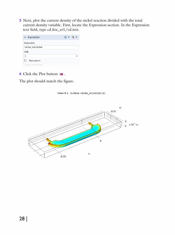
5 Next, plot the current density of the nickel reaction divided with the total current density variable. First, locate the Expression section. In the Expression text field, type cd.iloc_er1/cd.itot.

6 Click the Plot button .

The plot should match the figure.

28 |

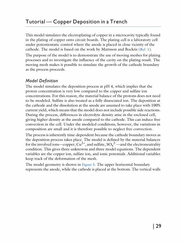
Tutorial — Copper Deposition in a Trench

This model simulates the electroplating of copper in a microcavity typically found in the plating of copper onto circuit boards. The plating cell is a laboratory cell under potentiostatic control where the anode is placed in close vicinity of the cathode. The model is based on the work by Mattsson and Bockris (Ref. 1). The purpose of the model is to demonstrate the use of moving meshes for plating processes and to investigate the influence of the cavity on the plating result. The moving mesh makes it possible to simulate the growth of the cathode boundary as the process proceeds.

Model DefinitionThe model simulates the deposition process at pH 4, which implies that the proton concentration is very low compared to the copper and sulfate ion concentrations. For this reason, the material balance of the protons does not need to be modeled. Sulfate is also treated as a fully dissociated ion. The deposition at the cathode and the dissolution at the anode are assumed to take place with 100% current yield, which means that the model does not include possible side reactions. During the process, differences in electrolyte density arise in the enclosed cell, giving higher density at the anode compared to the cathode. This can induce free convection in the cell. Under the modeled conditions, however, the variations in composition are small and it is therefore possible to neglect free convection.The process is inherently time-dependent because the cathode boundary moves as the deposition process takes place. The model is defined by the material balances for the involved ions—copper, Cu2+, and sulfate, SO4

2-—and the electroneutrality condition. This gives three unknowns and three model equations. The dependent variables are the copper ion, sulfate ion, and ionic potentials. Additional variables keep track of the deformation of the mesh.The model geometry is shown in Figure 5. The upper horizontal boundary represents the anode, while the cathode is placed at the bottom. The vertical walls

| 29

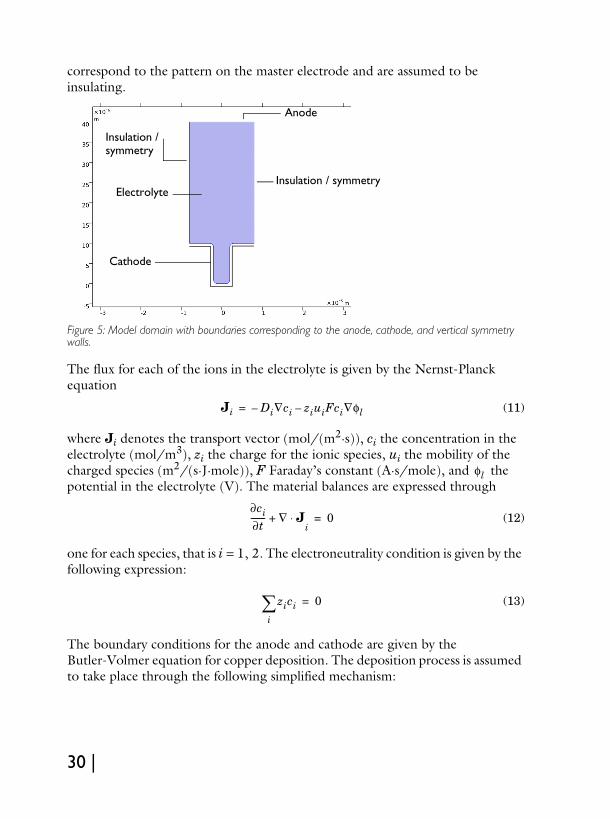
correspond to the pattern on the master electrode and are assumed to be insulating.

Figure 5: Model domain with boundaries corresponding to the anode, cathode, and vertical symmetry walls.

The flux for each of the ions in the electrolyte is given by the Nernst-Planck equation

(11)

where Ji denotes the transport vector (mol/(m2·s)), ci the concentration in the electrolyte (mol/m3), zi the charge for the ionic species, ui the mobility of the charged species (m2/(s·J·mole)), F Faraday’s constant (A·s/mole), and the potential in the electrolyte (V). The material balances are expressed through

(12)

one for each species, that is i = 1, 2. The electroneutrality condition is given by the following expression:

(13)

The boundary conditions for the anode and cathode are given by the Butler-Volmer equation for copper deposition. The deposition process is assumed to take place through the following simplified mechanism:

Insulation / symmetry

Cathode

Anode

Electrolyte

Insulation /symmetry

Ji Di∇ci– ziuiFci∇φl–=

φl

∂ci

∂t------- ∇ J⋅+

i0=

zici

i 0=

30 |

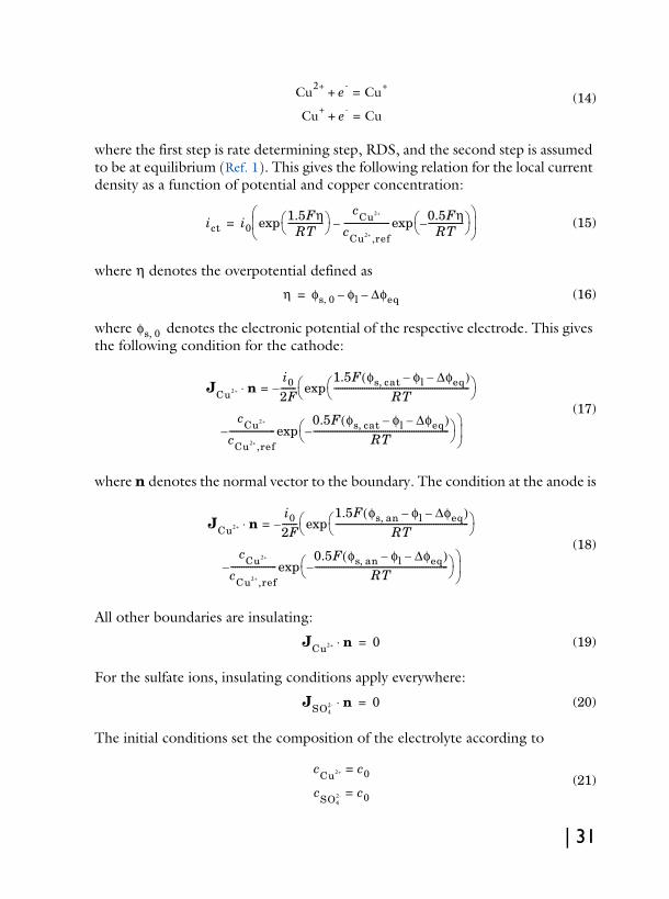
(14)

where the first step is rate determining step, RDS, and the second step is assumed to be at equilibrium (Ref. 1). This gives the following relation for the local current density as a function of potential and copper concentration:

(15)

where η denotes the overpotential defined as

(16)

where denotes the electronic potential of the respective electrode. This gives the following condition for the cathode:

(17)

where n denotes the normal vector to the boundary. The condition at the anode is

(18)

All other boundaries are insulating:

(19)

For the sulfate ions, insulating conditions apply everywhere:

(20)

The initial conditions set the composition of the electrolyte according to

(21)

Cu2+ e-+ Cu+

=

Cu+ e-+ Cu=

ict i01.5Fη

RT----------------

cCu2+

cCu2+,ref

--------------------- 0.5FηRT----------------–

exp–exp

=

η φs 0, φl– Δφeq–=

φs 0,

JCu2+ n⋅i02F-------–

1.5F φs cat, φl– Δφeq–( )RT

-------------------------------------------------------------- exp

=

cCu2+

cCu2+,ref

---------------------0.5F φs cat, φl– Δφeq–( )

RT--------------------------------------------------------------–

exp

–

JCu2+ n⋅i02F-------–

1.5F φs an, φl– Δφeq–( )RT

------------------------------------------------------------- exp

=

cCu2+

cCu2+ ,ref

---------------------0.5F φs an, φl– Δφeq–( )

RT-------------------------------------------------------------–

exp

–

JCu2+ n⋅ 0=

JSO42- n⋅ 0=

cCu2+ c0=

cSO42- c0=

| 31

You set up Equation 11 through Equation 21 using the Tertiary Current Distribution, Nernst-Planck interface. The Deformed Geometry interface keeps track of the deformation of the mesh.Using the Electrode Surface boundary node, the ion fluxes and the boundary mesh velocity are based on the reaction currents, the number of electrons, and the specified stoichiometric coefficients of the electrode reactions. The sign of the stoichiometric coefficient for a species depends on whether the species is getting oxidized (positive) or reduced (negative) in the reaction. In the case for the total reaction in this model

the stoichiometric coefficient is for the copper ions in the electrolyte, and for the copper atoms in the electrodes.

Results and DiscussionFigure 6 shows the concentration distribution of copper ions, the isopotential lines, the current density lines, and the displacement of the cathode and anode surfaces after 14 seconds of operation. The figure shows that the mouth of the cavity is narrower due to the nonuniform thickness of the deposition. This effect can be detrimental to the quality of the deposition because a trapped electrolyte can later cause corrosion of components in the circuit board. In addition, the simulation shows substantial variations in copper ion concentration in the cell. Such variations eventually cause free convection in the cell. The model is symmetric along a

Cu2+ 2e-+ Cu=

νCu2+ 1–=νCu 1=

32 |

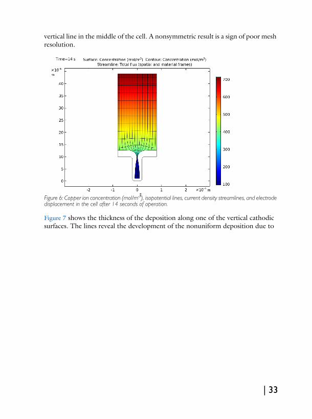
vertical line in the middle of the cell. A nonsymmetric result is a sign of poor mesh resolution.

Figure 6: Copper ion concentration (mol/m3), isopotential lines, current density streamlines, and electrode displacement in the cell after 14 seconds of operation.

Figure 7 shows the thickness of the deposition along one of the vertical cathodic surfaces. The lines reveal the development of the nonuniform deposition due to

| 33

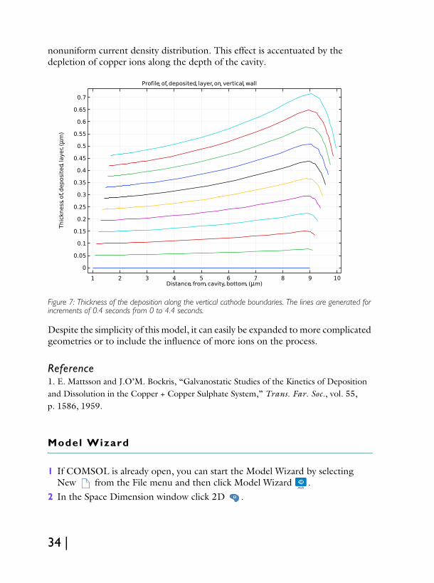
nonuniform current density distribution. This effect is accentuated by the depletion of copper ions along the depth of the cavity.

Figure 7: Thickness of the deposition along the vertical cathode boundaries. The lines are generated for increments of 0.4 seconds from 0 to 4.4 seconds.

Despite the simplicity of this model, it can easily be expanded to more complicated geometries or to include the influence of more ions on the process.

Reference1. E. Mattsson and J.O’M. Bockris, “Galvanostatic Studies of the Kinetics of Deposition and Dissolution in the Copper + Copper Sulphate System,” Trans. Far. Soc., vol. 55, p. 1586, 1959.

Model Wizard

1 If COMSOL is already open, you can start the Model Wizard by selecting New from the File menu and then click Model Wizard .

2 In the Space Dimension window click 2D .

34 |

3 In the Select Physics tree under Electrochemistry>Electrodeposition, Deformed Geometry click Electrodeposition, Tertiary with Electroneutrality .

4 Click Add then click the Study button.5 In the tree under Preset Studies click Time Dependent with Initialization .6 Click Done .

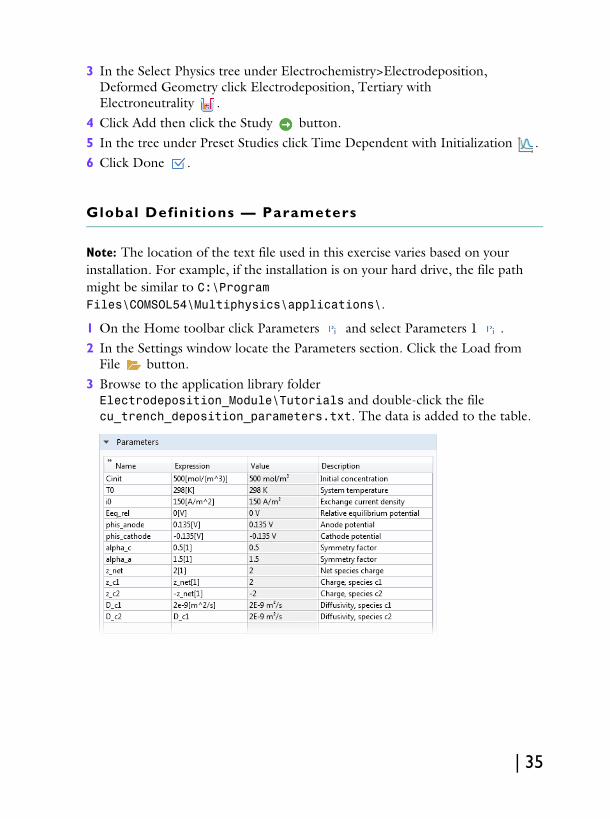
Global Definit ions — Parameters

Note: The location of the text file used in this exercise varies based on your installation. For example, if the installation is on your hard drive, the file path might be similar to C:\Program Files\COMSOL54\Multiphysics\applications\.

1 On the Home toolbar click Parameters and select Parameters 1 .2 In the Settings window locate the Parameters section. Click the Load from

File button.3 Browse to the application library folder Electrodeposition_Module\Tutorials and double-click the file cu_trench_deposition_parameters.txt. The data is added to the table.

| 35

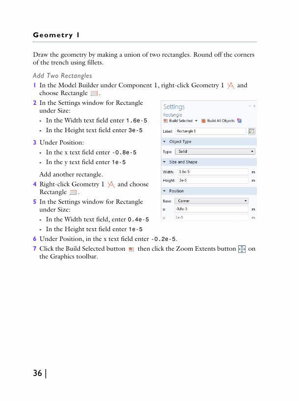
Geometry 1

Draw the geometry by making a union of two rectangles. Round off the corners of the trench using fillets.

Add Two Rectangles1 In the Model Builder under Component 1, right-click Geometry 1 and

choose Rectangle .2 In the Settings window for Rectangle

under Size:- In the Width text field enter 1.6e-5- In the Height text field enter 3e-5

3 Under Position:- In the x text field enter -0.8e-5- In the y text field enter 1e-5

Add another rectangle. 4 Right-click Geometry 1 and choose

Rectangle . 5 In the Settings window for Rectangle

under Size:- In the Width text field, enter 0.4e-5- In the Height text field enter 1e-5

6 Under Position, in the x text field enter -0.2e-5. 7 Click the Build Selected button then click the Zoom Extents button on

the Graphics toolbar.

36 |

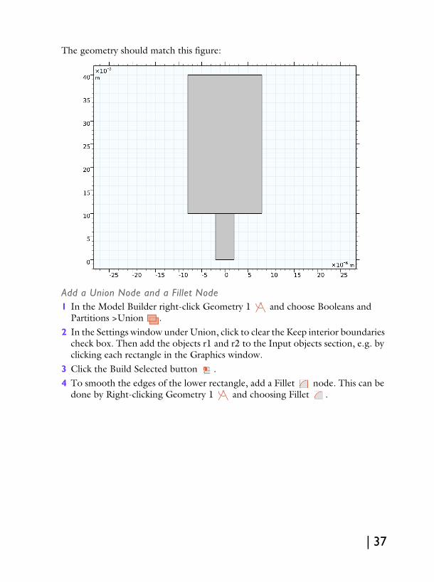
The geometry should match this figure:

Add a Union Node and a Fillet Node1 In the Model Builder right-click Geometry 1 and choose Booleans and

Partitions >Union .2 In the Settings window under Union, click to clear the Keep interior boundaries

check box. Then add the objects r1 and r2 to the Input objects section, e.g. by clicking each rectangle in the Graphics window.

3 Click the Build Selected button .4 To smooth the edges of the lower rectangle, add a Fillet node. This can be

done by Right-clicking Geometry 1 and choosing Fillet .

| 37

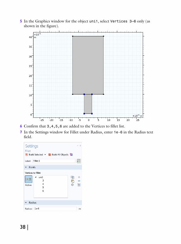
5 In the Graphics window for the object uni1, select Vertices 3–6 only (as shown in the figure).

6 Confirm that 3,4,5,6 are added to the Vertices to fillet list. 7 In the Settings window for Fillet under Radius, enter 1e-6 in the Radius text

field.

38 |

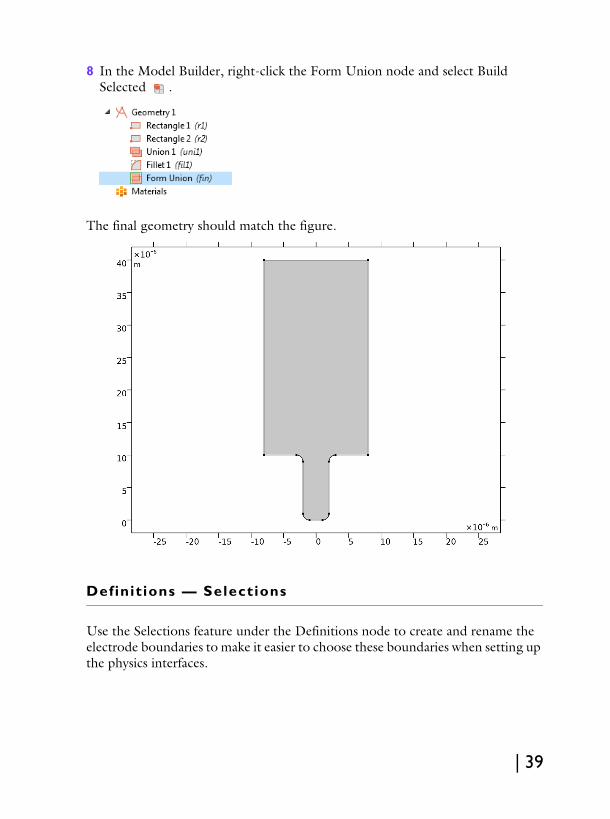
8 In the Model Builder, right-click the Form Union node and select Build Selected .

The final geometry should match the figure.

Definit ions — Selections

Use the Selections feature under the Definitions node to create and rename the electrode boundaries to make it easier to choose these boundaries when setting up the physics interfaces.

| 39

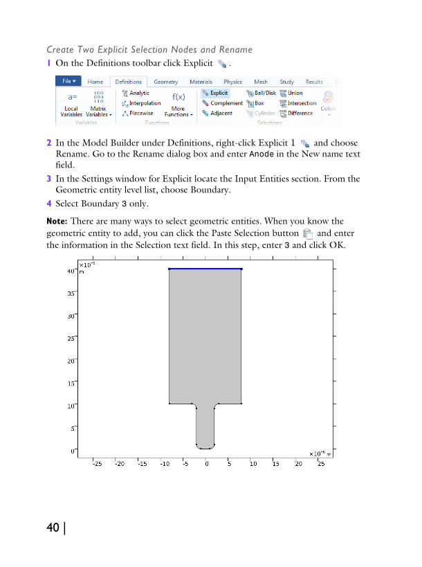
Create Two Explicit Selection Nodes and Rename1 On the Definitions toolbar click Explicit .

2 In the Model Builder under Definitions, right-click Explicit 1 and choose Rename. Go to the Rename dialog box and enter Anode in the New name text field.

3 In the Settings window for Explicit locate the Input Entities section. From the Geometric entity level list, choose Boundary.

4 Select Boundary 3 only.

Note: There are many ways to select geometric entities. When you know the geometric entity to add, you can click the Paste Selection button and enter the information in the Selection text field. In this step, enter 3 and click OK.

40 |

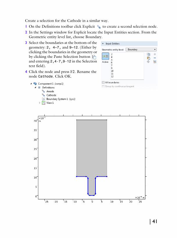
Create a selection for the Cathode in a similar way.1 On the Definitions toolbar click Explicit to create a second selection node.2 In the Settings window for Explicit locate the Input Entities section. From the

Geometric entity level list, choose Boundary.3 Select the boundaries at the bottom of the

geometry: 2, 4–7, and 9–12. (Either by clicking the boundaries in the geometry or by clicking the Paste Selection button and entering 2,4-7,9-12 in the Selection text field).

4 Click the node and press F2. Rename the node Cathode. Click OK.

| 41

Tertiary Current Distribution, Nernst-Planck

Now set up the electrochemical model, which consists of an electrolyte domain and two electrode boundaries.

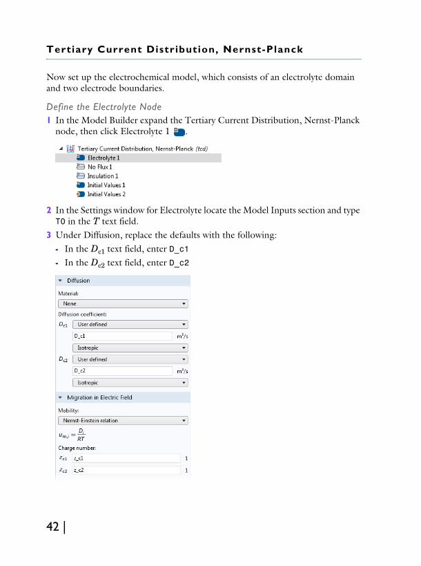
Define the Electrolyte Node1 In the Model Builder expand the Tertiary Current Distribution, Nernst-Planck

node, then click Electrolyte 1 .

2 In the Settings window for Electrolyte locate the Model Inputs section and type T0 in the T text field.

3 Under Diffusion, replace the defaults with the following:- In the Dc1 text field, enter D_c1- In the Dc2 text field, enter D_c2

42 |

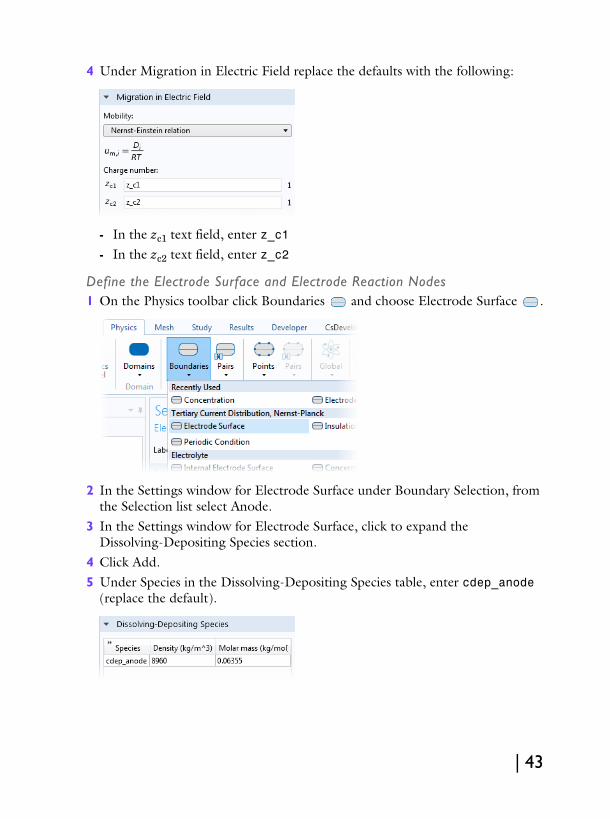
4 Under Migration in Electric Field replace the defaults with the following:

- In the zc1 text field, enter z_c1- In the zc2 text field, enter z_c2

Define the Electrode Surface and Electrode Reaction Nodes1 On the Physics toolbar click Boundaries and choose Electrode Surface .

2 In the Settings window for Electrode Surface under Boundary Selection, from the Selection list select Anode.

3 In the Settings window for Electrode Surface, click to expand the Dissolving-Depositing Species section.

4 Click Add. 5 Under Species in the Dissolving-Depositing Species table, enter cdep_anode

(replace the default).

| 43

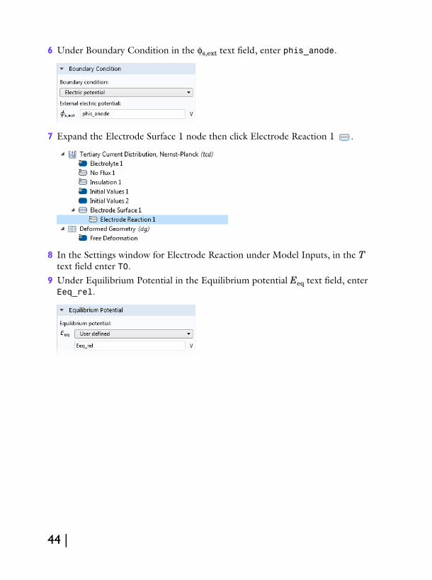
6 Under Boundary Condition in the φs,ext text field, enter phis_anode.

7 Expand the Electrode Surface 1 node then click Electrode Reaction 1 .

8 In the Settings window for Electrode Reaction under Model Inputs, in the T text field enter T0.

9 Under Equilibrium Potential in the Equilibrium potential Eeq text field, enter Eeq_rel.

44 |

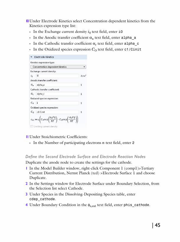
10Under Electrode Kinetics select Concentration dependent kinetics from the Kinetics expression type list:- In the Exchange current density i0 text field, enter i0- In the Anodic transfer coefficient αa text field, enter alpha_a- In the Cathodic transfer coefficient αc text field, enter alpha_c- In the Oxidized species expression CO text field, enter c1/Cinit

11Under Stoichiometric Coefficients:- In the Number of participating electrons n text field, enter 2

Define the Second Electrode Surface and Electrode Reaction NodesDuplicate the anode node to create the settings for the cathode. 1 In the Model Builder window, right-click Component 1 (comp1)>Tertiary

Current Distribution, Nernst Planck (tcd) >Electrode Surface 1 and choose Duplicate.

2 In the Settings window for Electrode Surface under Boundary Selection, from the Selection list select Cathode.

3 Under Species in the Dissolving-Depositing Species table, enter cdep_cathode.

4 Under Boundary Condition in the φs,ext text field, enter phis_cathode.

| 45

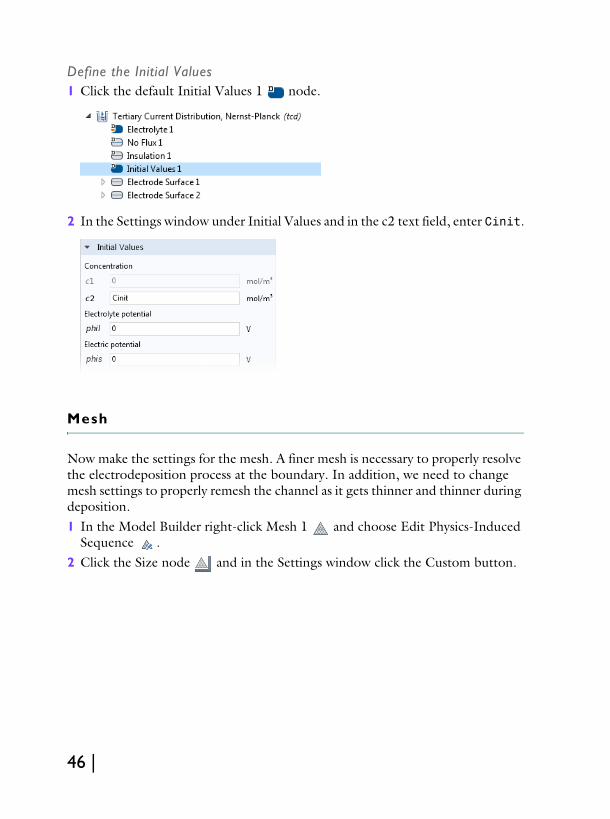
Define the Initial Values1 Click the default Initial Values 1 node.

2 In the Settings window under Initial Values and in the c2 text field, enter Cinit.

Mesh

Now make the settings for the mesh. A finer mesh is necessary to properly resolve the electrodeposition process at the boundary. In addition, we need to change mesh settings to properly remesh the channel as it gets thinner and thinner during deposition.1 In the Model Builder right-click Mesh 1 and choose Edit Physics-Induced

Sequence .2 Click the Size node and in the Settings window click the Custom button.

46 |

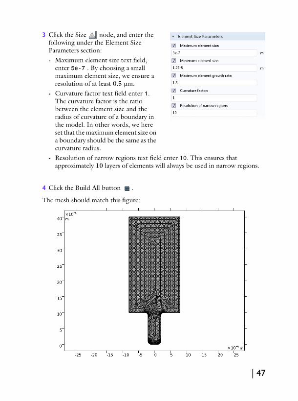
3 Click the Size node, and enter the following under the Element Size Parameters section:- Maximum element size text field,

enter 5e-7 . By choosing a small maximum element size, we ensure a resolution of at least 0.5 µm.

- Curvature factor text field enter 1. The curvature factor is the ratio between the element size and the radius of curvature of a boundary in the model. In other words, we here set that the maximum element size on a boundary should be the same as the curvature radius.

- Resolution of narrow regions text field enter 10. This ensures that approximately 10 layers of elements will always be used in narrow regions.

4 Click the Build All button .

The mesh should match this figure:

| 47

Study 1

Modify the times for the solver to simulate the deposition process during 5 s, storing the solution every 0.5 s. Then start the computation.1 In the Model Builder expand the Study 1 node then click Step 2: Time

Dependent .2 In the Settings window under Study Settings and in the Times text field, enter range(0,0.5,5).

3 On the Study toolbar click Compute .

It only takes a few moments for the default plot and Solver Configurations nodes to be added to the Model Builder and for the plots to display in the Graphics window.

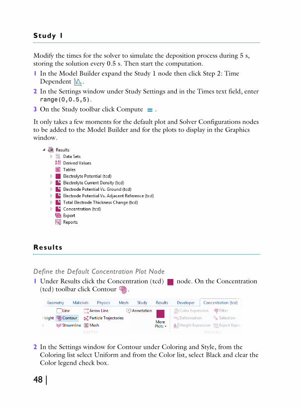
Results

Define the Default Concentration Plot Node1 Under Results click the Concentration (tcd) node. On the Concentration

(tcd) toolbar click Contour .

2 In the Settings window for Contour under Coloring and Style, from the Coloring list select Uniform and from the Color list, select Black and clear the Color legend check box.

48 |

3 On the Concentration (tcd) toolbar click Streamline .4 In the upper-right corner of the Expression section, click the Replace

Expression button.5 From the menu choose Tertiary Current Distribution, Nernst Planck >

tcd.tflux_c1x,tcd.tflxu_c1y - Total flux (spatial and material frames).

6 From the Selection list choose anode.7 Under Streamline Positioning and from the Positioning list, choose On selected

boundaries. In the Number text field, enter 15.8 On the Concentration (tcd) toolbar click Line .

9 Under Data, choose Study1/Solution 1 as the Data set and set Time(s) to the first value (0 s).

10Under Coloring and Style, from the Coloring list select Uniform. From the Color list select Black.

11Click the Plot button .

| 49

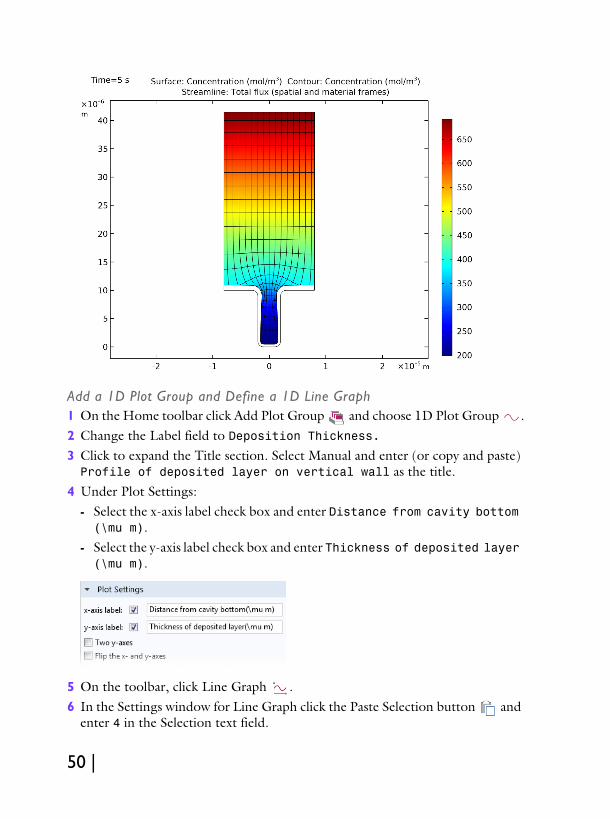
Add a 1D Plot Group and Define a 1D Line Graph1 On the Home toolbar click Add Plot Group and choose 1D Plot Group .2 Change the Label field to Deposition Thickness.3 Click to expand the Title section. Select Manual and enter (or copy and paste) Profile of deposited layer on vertical wall as the title.

4 Under Plot Settings:- Select the x-axis label check box and enter Distance from cavity bottom (\mu m).

- Select the y-axis label check box and enter Thickness of deposited layer (\mu m).

5 On the toolbar, click Line Graph .6 In the Settings window for Line Graph click the Paste Selection button and

enter 4 in the Selection text field.

50 |

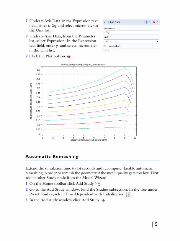
7 Under y-Axis Data, in the Expression text field, enter x-Xg and select micrometer in the Unit list.

8 Under x-Axis Data, from the Parameter list, select Expression. In the Expression text field, enter y and select micrometer in the Unit list.

9 Click the Plot button .

Automatic Remeshing

Extend the simulation time to 14 seconds and recompute. Enable automatic remeshing in order to remesh the geometry if the mesh quality gets too low. First, add another Study node from the Model Wizard.1 On the Home toolbar click Add Study . 2 Go to the Add Study window. Find the Studies subsection. In the tree under

Preset Studies, select Time Dependent with Initialization .3 In the Add study window click Add Study .

| 51

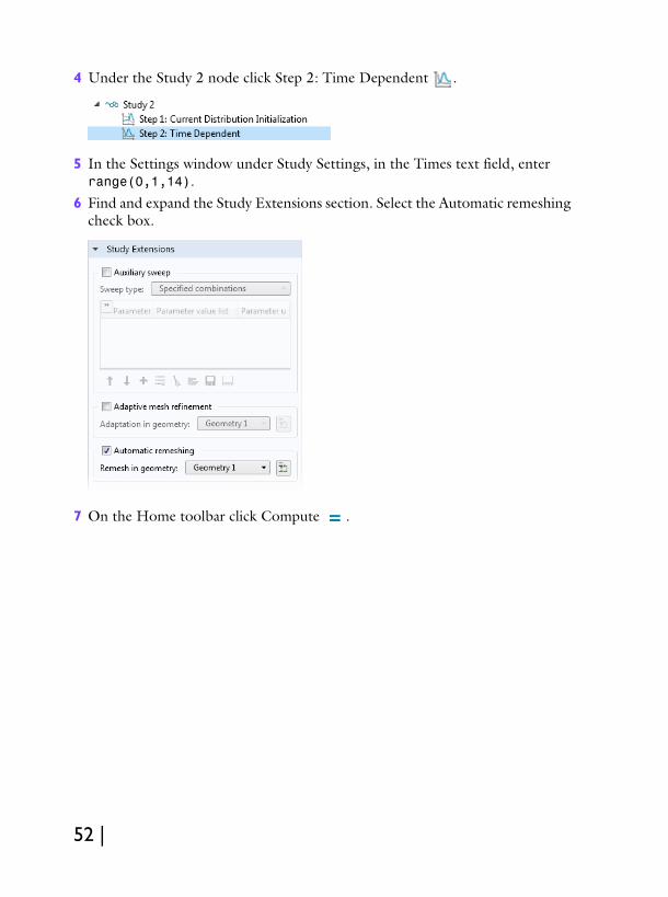
4 Under the Study 2 node click Step 2: Time Dependent .

5 In the Settings window under Study Settings, in the Times text field, enter range(0,1,14).

6 Find and expand the Study Extensions section. Select the Automatic remeshing check box.

7 On the Home toolbar click Compute .

52 |

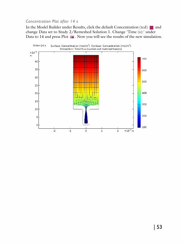
Concentration Plot after 14 sIn the Model Builder under Results, click the default Concentration (tcd) and change Data set to Study 2/Remeshed Solution 1. Change 'Time (s):' under Data to 14 and press Plot . Now you will see the results of the new simulation.

| 53

54 |