Introduction to SVMs

8/20/2019 Introduction to SVMs

http://slidepdf.com/reader/full/introduction-to-svms 1/38

Chapter 7

An Introduction to Kernel Methods

C. Campbell

Kernel methods give a systematic and principled approach to training

learning machines and the good generalization performance achieved

can be readily justified using statistical learning theory or Bayesian ar-

guments. We describe how to use kernel methods for classification, re-

gression and novelty detection and in each case we find that training can

be reduced to optimization of a convex cost function. We describe al-

gorithmic approaches for training these systems including model selec-

tion strategies and techniques for handling unlabeled data. Finally we

present some recent applications. The emphasis will be on using RBF

kernels which generate RBF networks but the approach is general since

other types of learning machines (e.g., feed-forward neural networks or

polynomial classifiers) can be readily generated with different choices of

kernel.

1 Introduction

Radial Basis Function (RBF) networks have been widely studied because

they exhibit good generalization and universal approximation through

use of RBF nodes in the hidden layer. In this Chapter we will outline

a new approach to designing RBF networks based on kernel methods.

These techniques have a number of advantages. As we shall see, the ap-

proach is systematic and properly motivated theoretically. The learning

machine is also explicitly constructed using the most informative pat-

terns in the data. Because the dependence on the data is clear it is much

easier to explain and interpret the model and data cleaning [16] could

be implemented to improve performance. The learning process involves

optimization of a cost function which is provably convex. This contrasts

with neural network approaches where the exist of false local minima in

the error function can complicate the learning process. For kernel meth-

155



156 Chapter 7

ods there are comparatively few parameters required for tuning the sys-tem. Indeed, recently proposed model selection schemes could lead to

the elimination of these parameters altogether. Unlike neural network ap-

proaches the architecture is determined by the algorithm and not found

by experimentation. It is also possible to give confidence estimates on

the classification accuracy on new test examples. Finally these learning

machines typically exhibit good generalization and perform well in prac-

tice.

In this introduction to the subject, we will focus on Support Vector Ma-

chines (SVMs) which are the most well known learning systems basedon kernel methods. The emphasis will be on classification, regression and

novelty detection and we will not cover other interesting topics, for exam-

ple, kernel methods for unsupervised learning [43], [52]. We will begin

by introducing SVMs for binary classification and the idea of kernel sub-

stitution. The kernel representation of data amounts to a nonlinear pro-

jection of data into a high-dimensional space where it is easier to separate

the two classes of data. We then develop this approach to handle noisy

datasets, multiclass classification, regression and novelty detection. We

also consider strategies for finding the kernel parameter and techniques

for handling unlabeled data. In Section 3, we then describe algorithms for

training these systems and in Section 4, we describe some current appli-

cations. In the conclusion, we will briefly discuss other types of learning

machines based on kernel methods.

2 Kernel Methods for Classification,

Regression, and Novelty Detection

2.1 Binary Classification

From the perspective of statistical learning theory the motivation for con-

sidering binary classifier SVMs comes from theoretical bounds on the

generalization error [58], [59], [10]. For ease of explanation we give the

theorem in the Appendix 1 (Theorem 1) and simply note here that it has

two important features. Firstly, the error bound is minimized by maxi-

mizing the margin, , i.e., the minimal distance between the hyperplane

separating the two classes and the closest datapoints to the hyperplane



An Introduction to Kernel Methods 157

x1 x2

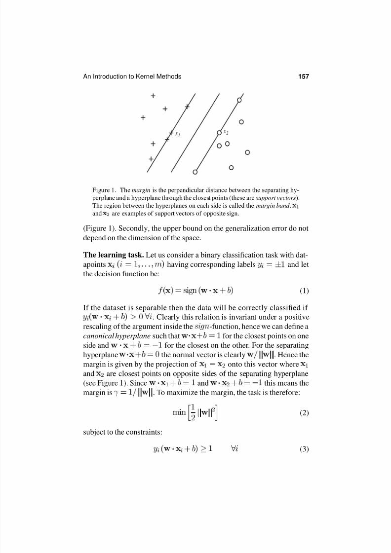
Figure 1. The margin is the perpendicular distance between the separating hy-

perplane and a hyperplane through the closest points (these are support vectors).

The region between the hyperplanes on each side is called the margin band .

and

are examples of support vectors of opposite sign.

(Figure 1). Secondly, the upper bound on the generalization error do not

depend on the dimension of the space.

The learning task. Let us consider a binary classification task with dat-

apoints

having corresponding labels

and let

the decision function be:

(1)

If the dataset is separable then the data will be correctly classified if

. Clearly this relation is invariant under a positive

rescaling of the argument inside the -function, hence we can define a

canonical hyperplane such that for the closest points on one

side and

for the closest on the other. For the separating

hyperplane the normal vector is clearly . Hence the

margin is given by the projection of

onto this vector where

and

are closest points on opposite sides of the separating hyperplane

(see Figure 1). Since

and

this means the

margin is . To maximize the margin, the task is therefore:

(2)

subject to the constraints:

(3)



158 Chapter 7

and the learning task reduces to minimization of the primal objectivefunction:

(4)

where

are Lagrange multipliers (hence

. Taking the derivatives

with respect to and gives:

(5)

(6)

and resubstituting these expressions back in the primal gives the Wolfe

dual:

(7)

which must be maximized with respect to the

subject to the constraint:

(8)

Kernel substitution. This constrained quadratic programming (QP)

problem will give an optimal separating hyperplane with a maximal mar-

gin if the data is separable. However, we have still not exploited the sec-

ond observation from theorem 1: the error bound does not depend on

the dimension of the space. This feature enables us to give an alternative

kernel representation of the data which is equivalent to a mapping into a

high dimensional space where the two classes of data are more readily

separable. This space is called feature space and must be a pre-Hilbert or

inner product space. For the dual objective function in (7) we notice that

the datapoints,

, only appear inside an inner product. Thus the mappingis achieved through a replacement of the inner product:

(9)

The functional form of the mapping

does not need to be known

since it is implicitly defined by the choice of kernel:

(10)




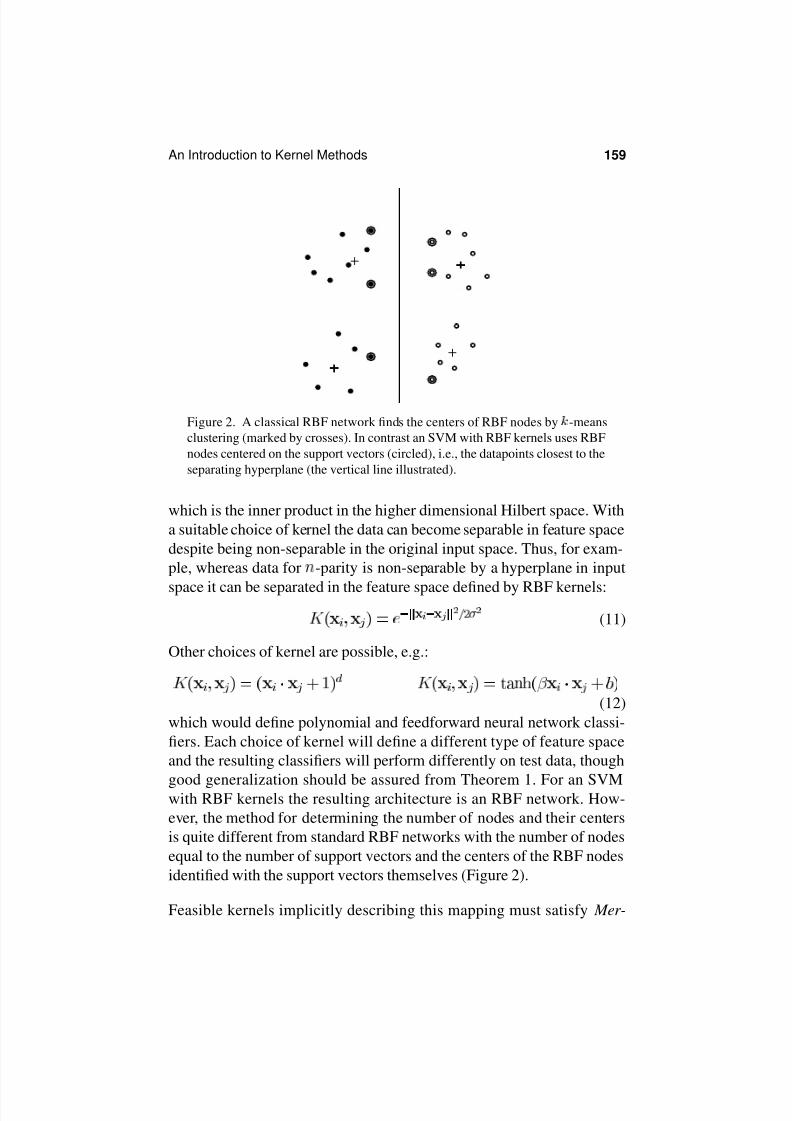
Figure 2. A classical RBF network finds the centers of RBF nodes by -means

clustering (marked by crosses). In contrast an SVM with RBF kernels uses RBF

nodes centered on the support vectors (circled), i.e., the datapoints closest to the

separating hyperplane (the vertical line illustrated).

which is the inner product in the higher dimensional Hilbert space. With

a suitable choice of kernel the data can become separable in feature space

despite being non-separable in the original input space. Thus, for exam-

ple, whereas data for -parity is non-separable by a hyperplane in input

space it can be separated in the feature space defined by RBF kernels:

(11)

Other choices of kernel are possible, e.g.:

(12)

which would define polynomial and feedforward neural network classi-

fiers. Each choice of kernel will define a different type of feature space

and the resulting classifiers will perform differently on test data, though

good generalization should be assured from Theorem 1. For an SVMwith RBF kernels the resulting architecture is an RBF network. How-

ever, the method for determining the number of nodes and their centers

is quite different from standard RBF networks with the number of nodes

equal to the number of support vectors and the centers of the RBF nodes

identified with the support vectors themselves (Figure 2).

Feasible kernels implicitly describing this mapping must satisfy Mer-



160 Chapter 7

cer’s conditions described in more detail in Appendix 2. The class of mathematical objects which can be used as kernels is very general and

includes, for example, scores produced by dynamic alignment algorithms

[18], [63] and a wide range of functions.

For the given choice of kernel the learning task therefore involves maxi-

mization of the objective function:

(13)

subject to the constraints of Equation (8). The associated Karush-Kuhn-

Tucker (KKT) conditions are:

(14)

which are always satisfied when a solution is found. Test examples are

evaluated using a decision function given by the sign of:

(15)

Since the bias, , does not feature in the above dual formulation it is

found from the primal constraints:

(16)

using the optimal values of

. When the maximal margin hyperplane

is found in feature space, only those points which lie closest to the hy-

perplane have

and these points are the support vectors (all other

points have

. This means that the representation of the hypoth-

esis is given solely by those points which are closest to the hyperplane

and they are the most informative patterns in the data. Patterns which are




1/3

2/3

321

1/2

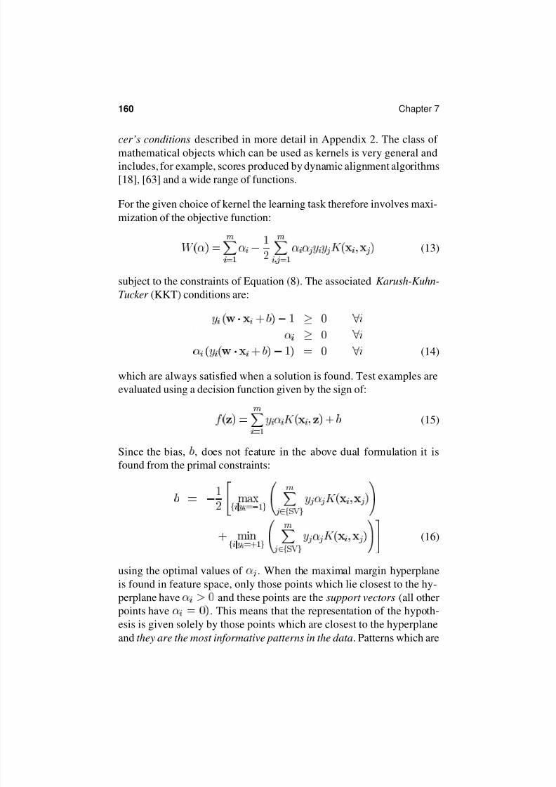
Figure 3. A multi-class classification problem can be reduced to a series of

binary classification tasks using a tree structure with a binary decision at eachnode.

not support vectors do not influence the position and orientation of the

separating hyperplane and so do not contribute to the hypothesis (Figure

1).

We have motivated SVMs using statistical learning theory but they can

also be understood from a Bayesian perspective [51], [25], [26]. Bayesian

[53] and statistical learning theory can also be used to define confidence

measures for classification. From the latter we find that the confidence

of a classification is directly related to the magnitude of on a testexample [46].

2.2 Multiclass Classification

Many real-life datasets involve multiclass classification and various

schemes have been proposed to handle this [28]. One approach is to

generalize the binary classifier to an class classifier with weights and

biases

for each class and a decision function [64]:

(17)

However, this type of classifier has a similar level of performance to

the simpler scheme of binary classifiers each of which performs one-

against-all classification. Binary classifiers can also be incorporated into

a directed acyclic graph (Figure 3) so that multiclass classification is de-

composed to binary classification at each node in the tree [34].



162 Chapter 7

2.3 Allowing for Training Errors: Soft MarginTechniques

Most real life datasets contain noise and an SVM can fit to this noise

leading to poor generalization. The effect of outliers and noise can be

reduced by introducing a soft margin [8] and two schemes are currently

used. In the first (

error norm) the learning task is the same as in Equa-

tions (13,8) except for the introduction of the box constraint:

(18)

while in the second (

error norm) the learning task is as in Equations

(13,8) except for addition of a small positive constant to the leading di-

agonal of the kernel matrix [8], [48]:

(19)

and control the trade-off between training error and generalization

ability and are chosen by means of a validation set. The effect of these

soft margins is illustrated in Figure 4 for the ionosphere dataset from the

UCI Repository [57].

The justification for these approaches comes from statistical learning the-

ory (cf. Theorems 2 and 3 in Appendix 1). Thus for the

error norm

(and prior to introducing kernels) condition (3) is relaxed by introducing

a positive slack variable

:

(20)

and the task is now to minimize the sum of errors

in addition to

:

(21)

This is readily formulated as a primal objective function:

(22)




with Lagrange multipliers

and

. The derivatives with re-spect to , and give:

(23)

(24)

(25)

Resubstituting these back in the primal objective function we obtain thesame dual objective function as before, Equation (13). However,

and

, hence

and the constraint

is replaced

by

. Patterns with values

will be referred to

later as non-bound and those with

or

will be said to be at

bound . For an

error norm we find the bias in the decision function of

Equation (15) by using the final KKT condition in Equation (14). Thus

if

is a non-bound pattern it follows that

assuming

.

The optimal value of must be found by experimentation using a vali-

dation set (Figure 4) and it cannot be readily related to the characteristics

of the dataset or model. In an alternative approach [44], a soft margin pa-

rameter, , can be interpreted as an upper bound on the fraction

of training errors and a lower bound on the fraction of patterns which are

support vectors.

For the

error norm the primal objective function is:

(26)

with

and

. After obtaining the derivatives with respect

to , and , substituting for and in the primal objective function

and noting that the dual objective function is maximal when

we



164 Chapter 7

5.2

5.4

5.6

5.8

6

6.2

6.4

6.6

6.8

7

7.2

0 5 10 15 20 25 30 35 40 45 50

5

5.5

6

6.5

7

7.5

0 0.2 0.4 0.6 0.8 1 1.2 1.4 1.6 1.8 2

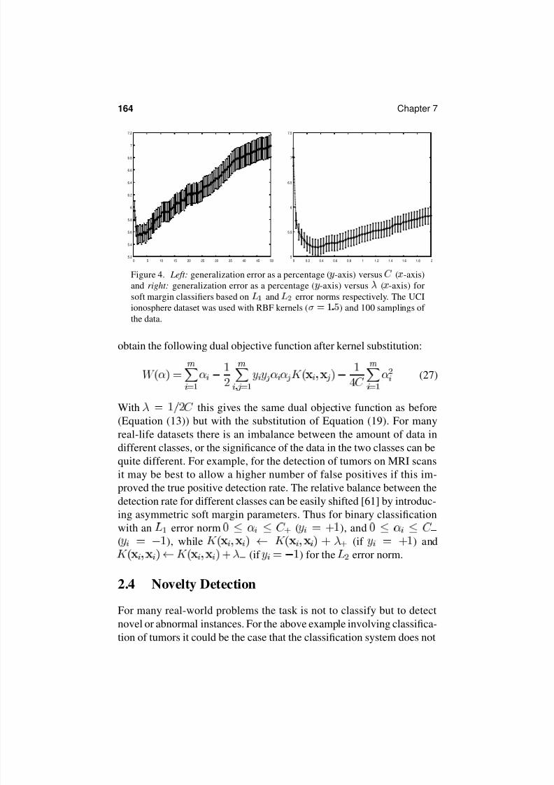
Figure 4. Left: generalization error as a percentage ( -axis) versus ( -axis)and right: generalization error as a percentage ( -axis) versus ( -axis) for

soft margin classifiers based on

and

error norms respectively. The UCI

ionosphere dataset was used with RBF kernels ( ) and 100 samplings of

the data.

obtain the following dual objective function after kernel substitution:

(27)

With

this gives the same dual objective function as before(Equation (13)) but with the substitution of Equation (19). For many

real-life datasets there is an imbalance between the amount of data in

different classes, or the significance of the data in the two classes can be

quite different. For example, for the detection of tumors on MRI scans

it may be best to allow a higher number of false positives if this im-

proved the true positive detection rate. The relative balance between the

detection rate for different classes can be easily shifted [61] by introduc-

ing asymmetric soft margin parameters. Thus for binary classification

with an

error norm

(

), and

(

), while

(if

) and

(if

) for the

error norm.

2.4 Novelty Detection

For many real-world problems the task is not to classify but to detect

novel or abnormal instances. For the above example involving classifica-

tion of tumors it could be the case that the classification system does not




correctly detect a tumor with a rare shape which is distinct from all mem-bers of the training set. On the other hand, a novelty detector would still

potentially highlight the object as abnormal. Novelty detection has poten-

tial applications in many problem domains such as condition monitoring

or medical diagnosis. Novelty detection can be viewed as modeling the

support of a data distribution (rather than having to find a real-valued

function for estimating the density of the data itself). Thus, at its sim-

plest level, the objective is to create a binary-valued function which is

positive in those regions of input space where the data predominantly

lies and negative elsewhere.

One approach [54] is to find a hypersphere with a minimal radius and

centre which contains most of the data: novel test points lie outside the

boundary of this hypersphere. The technique we now outline was origi-

nally suggested by Vapnik [58], [5], interpreted as a novelty detector by

Tax and Duin [54] and used by the latter authors for real life applications

[55]. The effect of outliers is reduced by using slack variables

to allow

for datapoints outside the sphere and the task is to minimize the volume

of the sphere and number of datapoints outside, i.e.,

subject to the constraints:

and

, and where controls the tradeoff between the two terms. The

primal objective function is then:

(28)

with

and

. After kernel substitution the dual formulation

amounts to maximization of:

(29)



166 Chapter 7

with respect to

and subject to

and

.If then at bound examples will occur with

and

these correspond to outliers in the training process. Having completed

the training process a test point

is declared novel if:

(30)

where

is first computed by finding an example which is non-bound

and setting this inequality to an equality.

An alternative approach has been developed by Scholkopf et al. [41].Suppose we restrict our attention to RBF kernels: in this case the data

lie in a region on the surface of a hypersphere in feature space since

from (11). The objective is therefore to

separate off this region from the surface region containing no data. This

is achieved by constructing a hyperplane which is maximally distant from

the origin with all datapoints lying on the opposite side from the origin

and such that

. This construction can be extended to allow

for outliers by introducing a slack variable

giving rise to the following

criterion:

(31)

subject to:

(32)

with

. The primal objective function is therefore:

(33)

and the derivatives:

(34)

(35)

(36)




Since

the derivative implies

.After kernel substitution the dual formulation involves minimization of:

(37)

subject to:

(38)

To determine the bias we find an example, say, which is non-bound (

and

are nonzero and

) and determine

from:

(39)

The support of the distribution is then modeled by the decision function:

(40)

In the above models, the parameter has a neat interpretation as an up-

per bound on the fraction of outliers and a lower bound of the fraction

of patterns which are support vectors [41]. Scholkopf et al. [41] provide

good experimental evidence in favor of this approach including the high-

lighting of abnormal digits in the USPS handwritten character dataset.

The method also works well for other types of kernel. This and the ear-

lier scheme for novelty detection can also be used with an

error norm

in which case the constraint

is removed and an addition

to the kernel diagonal (19) used instead.

2.5 Regression

For real-valued outputs the learning task can also be theoretically moti-

vated from statistical learning theory. Theorem 4 in Appendix 1 gives a

bound on the generalization error to within a margin tolerance . We can

visualize this as a band or tube of size around the hypothesis

function

and any points outside this tube can be viewed as training

errors (Figure 5).



168 Chapter 7

ξ

ε

y

x

z

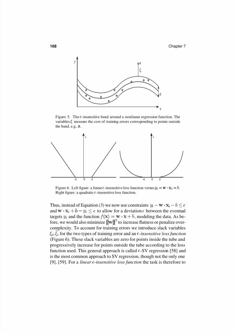
Figure 5. The -insensitive band around a nonlinear regression function. Thevariables measure the cost of training errors corresponding to points outside

the band, e.g., .

L

0 ε-ε

L

0 ε-ε

Figure 6. Left figure: a linear

-insensitive loss function versus

.

Right figure: a quadratic

-insensitive loss function.

Thus, instead of Equation (3) we now use constraints

and

to allow for a deviation between the eventual

targets

and the function , modeling the data. As be-

fore, we would also minimize

to increase flatness or penalize over-

complexity. To account for training errors we introduce slack variables

for the two types of training error and an

-insensitive loss function(Figure 6). These slack variables are zero for points inside the tube and

progressively increase for points outside the tube according to the loss

function used. This general approach is called -SV regression [58] and

is the most common approach to SV regression, though not the only one

[9], [59]. For a linear -insensitive loss function the task is therefore to




minimize:

(41)

subject to

(42)

where the slack variables are both positive

. After kernel substi-

tution the dual objective function is:

(43)

which is maximized subject to

(44)

and:

(45)

Similarly a quadratic -insensitive loss function gives rise to:

(46)

subject to (42), giving a dual objective function:

Æ

(47)

which is maximized subject to (44). The decision function is then:

(48)



170 Chapter 7

We still have to compute the bias, , and we do so by considering theKKT conditions for regression. For a linear loss function prior to kernel

substitution these are:

(49)

where

, and:

(50)

From the latter conditions we see that only when

or

are the slack variables non-zero: these examples correspond to points

outside the

-insensitive tube. Hence from Equation (49) we can find the

bias from a non-bound example with

using

and similarly for

we can obtain it from

.

Though the bias can be obtained from one such example it is best to

compute it using an average over all points on the margin.

From the KKT conditions we also deduce that

since

and

cannot be simultaneously non-zero because we would have non-zero

slack variables on both sides of the band. Thus, given that

is zero if

and vice versa, we can use a more convenient formulation for the

actual optimization task, e.g., maximize:

(51)

subject to

for a linear -insensitive loss function.

Apart from the formulations given here it is possible to define other loss

functions giving rise to different dual objective functions. In addition,rather than specifying a priori it is possible to specify an upper bound

( ) on the fraction of points lying outside the band and then

find

by optimizing over the primal objective function:

(52)

with acting as an additional parameter to minimize over [38].




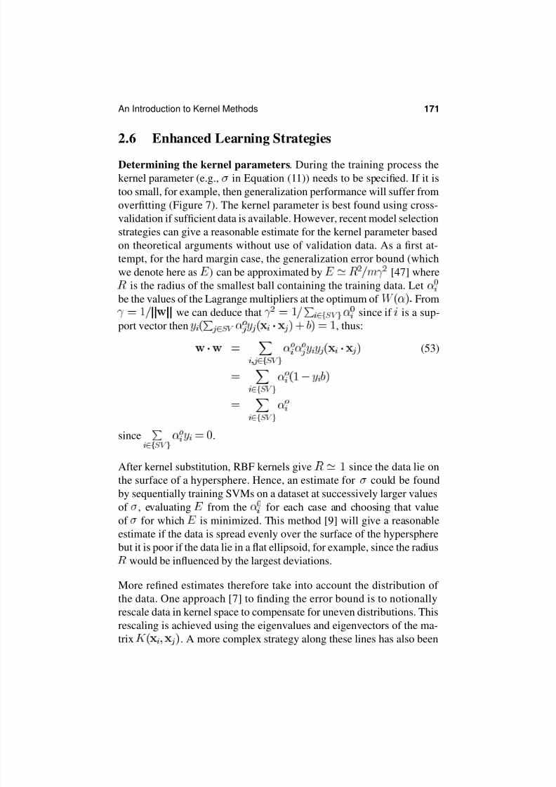
2.6 Enhanced Learning Strategies

Determining the kernel parameters. During the training process the

kernel parameter (e.g.,

in Equation (11)) needs to be specified. If it is

too small, for example, then generalization performance will suffer from

overfitting (Figure 7). The kernel parameter is best found using cross-

validation if sufficient data is available. However, recent model selection

strategies can give a reasonable estimate for the kernel parameter based

on theoretical arguments without use of validation data. As a first at-

tempt, for the hard margin case, the generalization error bound (which

we denote here as

) can be approximated by

[47] where

is the radius of the smallest ball containing the training data. Let

be the values of the Lagrange multipliers at the optimum of From

we can deduce that

since if is a sup-

port vector then

, thus:

(53)

since

.

After kernel substitution, RBF kernels give since the data lie on

the surface of a hypersphere. Hence, an estimate for

could be found

by sequentially training SVMs on a dataset at successively larger values

of , evaluating from the

for each case and choosing that value

of for which is minimized. This method [9] will give a reasonable

estimate if the data is spread evenly over the surface of the hypersphere

but it is poor if the data lie in a flat ellipsoid, for example, since the radius would be influenced by the largest deviations.

More refined estimates therefore take into account the distribution of

the data. One approach [7] to finding the error bound is to notionally

rescale data in kernel space to compensate for uneven distributions. This

rescaling is achieved using the eigenvalues and eigenvectors of the ma-

trix

. A more complex strategy along these lines has also been



172 Chapter 7

4

5

6

7

8

9

10

11

12

13

2 3 4 5 6 7 8 9 10

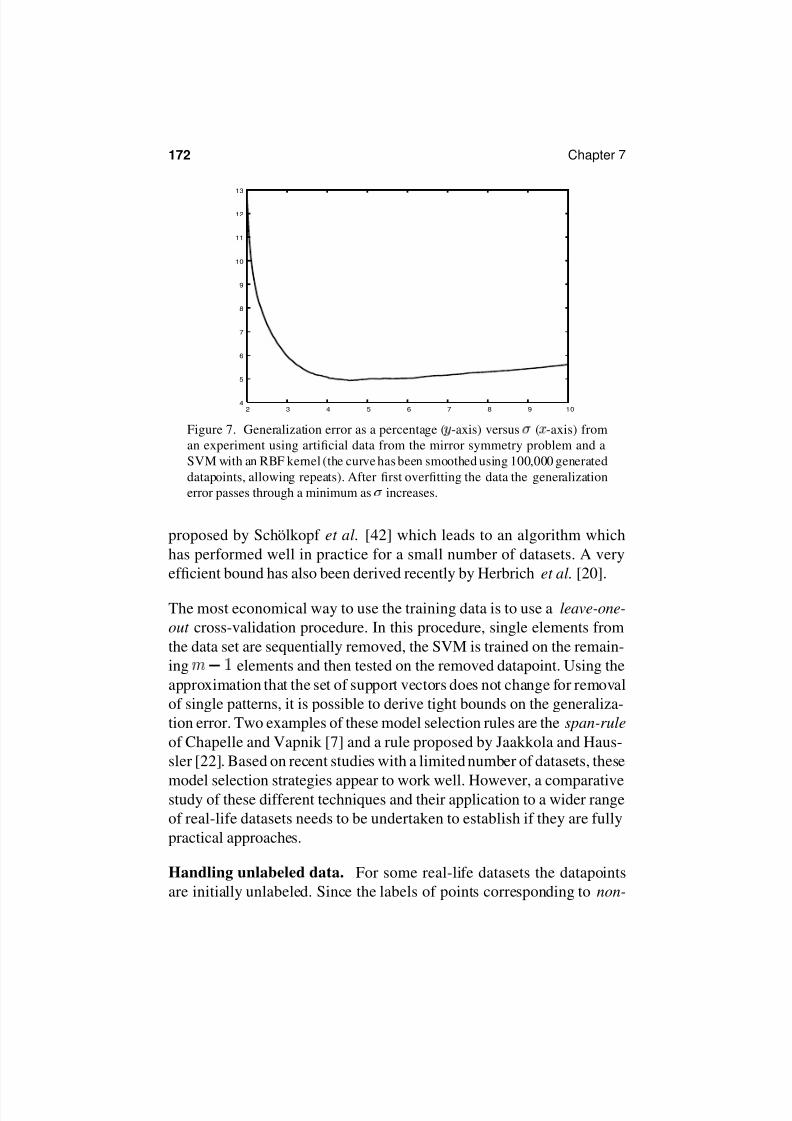
Figure 7. Generalization error as a percentage (

-axis) versus

(

-axis) from

an experiment using artificial data from the mirror symmetry problem and a

SVM with an RBF kernel (the curve has been smoothed using 100,000 generated

datapoints, allowing repeats). After first overfitting the data the generalization

error passes through a minimum as

increases.

proposed by Scholkopf et al. [42] which leads to an algorithm which

has performed well in practice for a small number of datasets. A very

efficient bound has also been derived recently by Herbrich et al. [20].

The most economical way to use the training data is to use a leave-one-

out cross-validation procedure. In this procedure, single elements from

the data set are sequentially removed, the SVM is trained on the remain-

ing elements and then tested on the removed datapoint. Using the

approximation that the set of support vectors does not change for removal

of single patterns, it is possible to derive tight bounds on the generaliza-

tion error. Two examples of these model selection rules are the span-rule

of Chapelle and Vapnik [7] and a rule proposed by Jaakkola and Haus-

sler [22]. Based on recent studies with a limited number of datasets, these

model selection strategies appear to work well. However, a comparativestudy of these different techniques and their application to a wider range

of real-life datasets needs to be undertaken to establish if they are fully

practical approaches.

Handling unlabeled data. For some real-life datasets the datapoints

are initially unlabeled. Since the labels of points corresponding to non-




0

5

10

15

20

25

30

35

40

0 20 40 60 80 100 120 140 160 180 200

0

500

1000

1500

2000

2500

3000

3500

4000

0 20 40 60 80 100 120 140 160 180 200

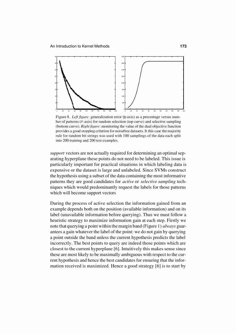
Figure 8. Left figure: generalization error ( -axis) as a percentage versus num-ber of patterns ( -axis) for random selection (top curve) and selective sampling

(bottom curve). Right figure: monitoring the value of the dual objective function

provides a good stopping criterion for noisefree datasets. It this case the majority

rule for random bit strings was used with 100 samplings of the data each split

into 200 training and 200 test examples.

support vectors are not actually required for determining an optimal sep-

arating hyperplane these points do not need to be labeled. This issue is

particularly important for practical situations in which labeling data is

expensive or the dataset is large and unlabeled. Since SVMs construct

the hypothesis using a subset of the data containing the most informativepatterns they are good candidates for active or selective sampling tech-

niques which would predominantly request the labels for those patterns

which will become support vectors

During the process of active selection the information gained from an

example depends both on the position (available information) and on its

label (unavailable information before querying). Thus we must follow a

heuristic strategy to maximize information gain at each step. Firstly we

note that querying a point within the margin band (Figure 1) always guar-

antees a gain whatever the label of the point: we do not gain by queryinga point outside the band unless the current hypothesis predicts the label

incorrectly. The best points to query are indeed those points which are

closest to the current hyperplane [6]. Intuitively this makes sense since

these are most likely to be maximally ambiguous with respect to the cur-

rent hypothesis and hence the best candidates for ensuring that the infor-

mation received is maximized. Hence a good strategy [6] is to start by



174 Chapter 7

requesting the labels for a small initial set of data and then successivelyquerying the labels of points closest to the current hyperplane. For noise-

free datasets, plateauing of the dual objective function provides a good

stopping criterion (since learning non-support vectors would not change

the value of

- see Figure 8(right)), whereas for noisy datasets emp-

tying of the margin band and a validation phase provide the best stopping

criterion [6]. Active selection works best if the hypothesis modeling the

data is sparse (i.e., there are comparatively few support vectors to be

found by the query learning strategy) in which case good generalization

is achieved despite requesting only a subset of labels in the dataset (Fig-

ure 8).

3 Algorithmic Approaches to Training

VMs

For classification, regression or novelty detection we see that the learn-

ing task involves optimization of a quadratic cost function and thus tech-

niques from quadratic programming are most applicable including quasi-

Newton, conjugate gradient and primal-dual interior point methods. Cer-

tain QP packages are readily applicable such as MINOS and LOQO.These methods can be used to train an SVM rapidly but they have the dis-

advantage that the kernel matrix is stored in memory. For small datasets

this is practical and QP routines are the best choice, but for larger datasets

alternative techniques have to be used. These split into two categories:

techniques in which kernel components are evaluated and discarded dur-

ing learning and working set methods in which an evolving subset of data

is used. For the first category the most obvious approach is to sequentially

update the

and this is the approach used by the Kernel Adatron (KA)

algorithm [15]. For binary classification (with no soft margin or bias) this

is a simple gradient ascent procedure on (13) in which

initially

and the

are subsequently sequentially updated using:

(54)

and

is the Heaviside step function. The optimal learning rate

can

be readily evaluated:

and a sufficient condition for con-

vergence is

. With the given decision function of




Equation (15), this method is very easy to implement and can give aquick impression of the performance of SVMs on classification tasks. It

is equivalent to Hildreth’s method in optimization theory and can be gen-

eralized to the case of soft margins and inclusion of a bias [27]. However,

it is not as fast as most QP routines, especially on small datasets.

3.1 Chunking and Decomposition

Rather than sequentially updating the

the alternative is to update the

in parallel but using only a subset or chunk of data at each stage.

Thus a QP routine is used to optimize the objective function on an initialarbitrary subset of data. The support vectors found are retained and all

other datapoints (with

) discarded. A new working set of data is

then derived from these support vectors and additional datapoints which

maximally violate the storage constraints. This chunking process is then

iterated until the margin is maximized. Of course, this procedure may still

fail because the dataset is too large or the hypothesis modeling the data is

not sparse (most of the

are non-zero, say). In this case decomposition

[31] methods provide a better approach: these algorithms only use a fixed

size subset of data with the

for the remainder kept fixed.

3.2 Decomposition and Sequential Minimal

Optimization

The limiting case of decomposition is the Sequential Minimal Optimiza-

tion (SMO) algorithm of Platt [33] in which only two

are optimized

at each iteration. The smallest set of parameters which can be optimized

with each iteration is plainly two if the constraint

is to hold.

Remarkably, if only two parameters are optimized and the rest kept fixed

then it is possible to derive an analytical solution which can be executed

using few numerical operations. The algorithm therefore selects two La-

grange multipliers to optimize at every step and separate heuristics are

used to find the two members of the pair. Due to its decomposition of the

learning task and speed it is probably the method of choice for training

SVMs and hence we will describe it in detail here for the case of binary

classification.



176 Chapter 7

The outer loop. The heuristic for the first member of the pair providesthe outer loop of the SMO algorithm. This loop iterates through the en-

tire training set to determining if an example violates the KKT conditions

and, if it does, to find if it is a candidate for optimization. After an initial

pass through the training set the outer loop does not subsequently iterate

through the entire training set. Instead it iterates through those examples

with Lagrange multipliers corresponding to non-bound examples (neither

nor ). Examples violating the KKT conditions are candidates for im-

mediate optimization and update. The outer loop makes repeated passes

over the non-bound examples until all of the non-bound examples obey

the KKT conditions. The outer loop then iterates over the entire trainingset again. The outer loop keeps alternating between single passes over

the entire training set and multiple passes over the non-bound subset un-

til the entire training set obeys the KKT conditions at which point the

algorithm terminates.

The inner loop. During the pass through the outer loop let us suppose

the algorithm finds an example which violates the KKT conditions (with

an associated Lagrange multiplier we shall denote

for convenience).

To find the second member of the pair,

, we proceed to the inner loop.

SMO selects the latter example to maximize the step-length taken during

the joint 2-variable optimization process outlined below. To achieve this

SMO keeps a record of each value of

(where

) for every non-bound example in the training set and then

approximates the step-length by the absolute value of the numerator in

equation (56) below, i.e.,

. Since we want to maximize the

step-length, this means we choose the minimum value of

if

is

positive and the maximum value of

if

is negative. As we point

out below, this step may not make an improvement. If so, SMO iterates

through the non-bound examples searching for a second example that

can make an improvement. If none of the non-bound examples gives an

improvement, then SMO iterates through the entire training set until anexample is found that makes an improvement. Both the iteration through

the non-bound examples and the iteration through the entire training set

are started at random locations to avoid an implicit bias towards examples

at the beginning of the training set.




The update rules. Having described the outer and inner loops for SMOwe now describe the rules used to update the chosen pair of Lagrange

multipliers (

). The constraint

gives:

(55)

Since

we have two possibilities. Firstly

in which case

is equal to some constant:

, say, or

in

which case

. The next step is to find the maximum of the

dual objective function with only two Lagrange multipliers permitted tochange. Usually this leads to a maximum along the direction of the linear

equality constraint though this not always the case as we discuss shortly.

We first determine the candidate value for second Lagrange multiplier

and then the ends of the diagonal line segment in terms of

:

(56)

where

and

(57)

If noise is present and we use a

soft margin then the next step is to

determine the two ends of the diagonal line segment. Thus if

the

following bounds apply:

(58)

and if

then:

(59)

The constrained maximum is then found by clipping the unconstrained

maximum to the ends of the line segment:

(60)



178 Chapter 7

Next the value of

is determined from the clipped

:

(61)

This operation moves

and

to the end point with the highest value

of

. Only when

is the same at both ends will no improve-

ment be made. After each step, the bias

is recomputed so that the KKT

conditions are fulfilled for both examples. If the new

is a non-bound

variable then

is determined from:

(62)

Similarly if the new

is non-bound then

is determined from:

(63)

If

and

are valid they should be equal. When both new Lagrange

multipliers are at bound and if is not equal to , then all thresholds

on the interval between

and

are consistent with the KKT conditions

and we choose the threshold to be halfway in between

and

.

The SMO algorithm has been refined to improve speed [24] and general-

ized to cover the above three tasks of classification [33], regression [49],

and novelty detection [41].

4 Applications

SVMs have been successfully applied to a number of applications rang-

ing from particle identification [2], face detection [32], and text catego-

rization [23], [13], [11] to engine knock detection [37], bioinformatics

[4], [65], and database marketing [3]. In this section, we discuss threesuccessful application areas as illustrations: machine vision, handwritten

character recognition and bioinformatics. This is a rapidly changing area

so more contemporary accounts are best obtained from relevant websites

(e.g., [17]).

Machine vision. SVMs are very suited to the binary or multiclass clas-

sification tasks which commonly arise in machine vision. As an example




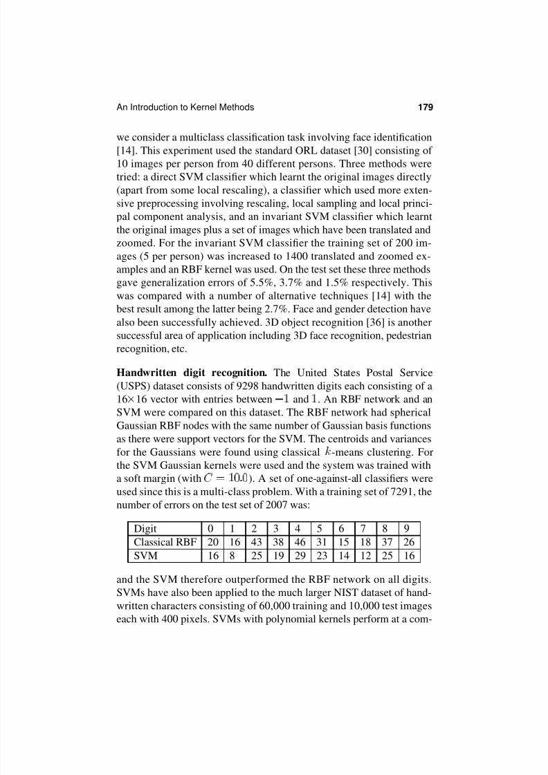
we consider a multiclass classification task involving face identification[14]. This experiment used the standard ORL dataset [30] consisting of

10 images per person from 40 different persons. Three methods were

tried: a direct SVM classifier which learnt the original images directly

(apart from some local rescaling), a classifier which used more exten-

sive preprocessing involving rescaling, local sampling and local princi-

pal component analysis, and an invariant SVM classifier which learnt

the original images plus a set of images which have been translated and

zoomed. For the invariant SVM classifier the training set of 200 im-

ages (5 per person) was increased to 1400 translated and zoomed ex-

amples and an RBF kernel was used. On the test set these three methodsgave generalization errors of 5.5%, 3.7% and 1.5% respectively. This

was compared with a number of alternative techniques [14] with the

best result among the latter being 2.7%. Face and gender detection have

also been successfully achieved. 3D object recognition [36] is another

successful area of application including 3D face recognition, pedestrian

recognition, etc.

Handwritten digit recognition. The United States Postal Service

(USPS) dataset consists of 9298 handwritten digits each consisting of a

16 16 vector with entries between and . An RBF network and an

SVM were compared on this dataset. The RBF network had spherical

Gaussian RBF nodes with the same number of Gaussian basis functions

as there were support vectors for the SVM. The centroids and variances

for the Gaussians were found using classical -means clustering. For

the SVM Gaussian kernels were used and the system was trained with

a soft margin (with ). A set of one-against-all classifiers were

used since this is a multi-class problem. With a training set of 7291, the

number of errors on the test set of 2007 was:

Digit 0 1 2 3 4 5 6 7 8 9

Classical RBF 20 16 43 38 46 31 15 18 37 26SVM 16 8 25 19 29 23 14 12 25 16

and the SVM therefore outperformed the RBF network on all digits.

SVMs have also been applied to the much larger NIST dataset of hand-

written characters consisting of 60,000 training and 10,000 test images

each with 400 pixels. SVMs with polynomial kernels perform at a com-



180 Chapter 7

parable level to the best alternative techniques [59] with an 0.8% erroron the test set.

Bioinformatics. Large-scale DNA sequencing projects are producing

large volumes of data and there is a considerable demand for sophis-

ticated methods for analyzing biosequences. Bioinformatics presents a

large number of important classification tasks such as prediction of pro-

tein secondary structure, classification of gene expression data, recog-

nizing splice junctions, i.e., the boundaries between exons and introns,

etc. SVMs have been found to be very effective on these tasks. For ex-

ample, SVMs outperformed four standard machine learning classifierswhen applied to the functional classification of genes using gene expres-

sion data from DNA microarray hybridization experiments [4]. Several

different similarity metrics and kernels were used and the best perfor-

mance was achieved using an RBF kernel (the dataset was very imbal-

anced so asymmetric soft margin parameters were used). A second suc-

cessful application has been protein homology detection to determine

the structural and functional properties of new protein sequences [21].

Determination of these properties is achieved by relating new sequences

to proteins with known structural features. In this application the SVM

outperformed a number of established systems for homology detection

for relating the test sequence to the correct families. As a third applica-

tion we also mention the detection of translation initiation sites [65] (the

points on nucleotide sequences where regions encoding proteins start).

SVMs performed very well on this task using a kernel function specifi-

cally designed to include prior biological information.

5 Conclusion

Kernel methods have many appealing features. We have seen that they

can be applied to a wide range of classification, regression and noveltydetection tasks but they can also be applied to other areas we have not

covered such as operator inversion and unsupervised learning. They can

be used to generate many possible learning machine architectures (RBF

networks, feedforward neural networks) through an appropriate choice

of kernel. In particular the approach is properly motivated theoretically

and systematic in execution.




Our focus has been on SVMs but the concept of kernel substitution of the inner product is a powerful idea separate from margin maximization

and it can be used to define many other types of learning machines which

can exhibit superior generalization [19], [29] or which use few patterns

to construct the hypothesis [56]. We have not been able to discuss these

here but they also perform well and appear very promising. The excellent

potential of this approach certainly suggests it will remain and develop

as an important set of tools for machine learning.

AcknowledgementsThe author would like to thank Nello Cristianini and Bernhard Scholkopf

for comments on an earlier draft.

Appendices

Appendix 1: Generalization Bounds

The generalization bounds mentioned in Section 2 are derived within the

framework of probably approximately correct or pac learning. The prin-cipal assumption governing this approach is that the training and test data

are independently and identically (iid) generated from a fixed distribution

denoted

. The distribution over input-output mappings will be denoted

and we will further assume that

is an inner

product space. With these assumptions pac-learnability can be described

as follows. Consider a class of possible target concepts and a learner

using a hypothesis space to try and learn this concept class. The

class is pac-learnable by if for any target concept , will with

probability Æ output a hypothesis with a generalization error

Æ

given a sufficient number,

, of training examplesand computation time. The pac bound Æ is derived using prob-

abilistic arguments [1], [62] and bounds the tail of the distribution of the

generalization error

.

For the case of a thresholding learner with unit weight vector on an

inner product space and a margin

the following theorem can

be derived if the dataset is linearly separable:



182 Chapter 7

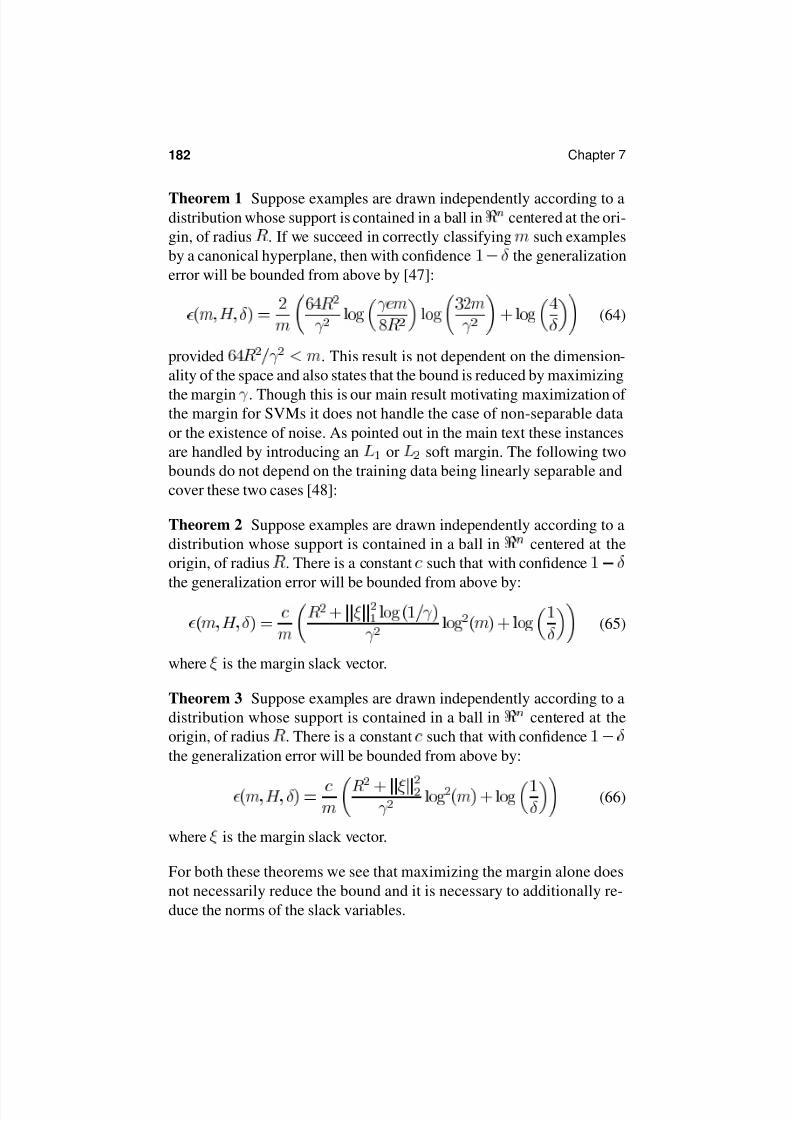
Theorem 1 Suppose examples are drawn independently according to adistribution whose support is contained in a ball in

centered at the ori-

gin, of radius . If we succeed in correctly classifying such examples

by a canonical hyperplane, then with confidence Æ

the generalization

error will be bounded from above by [47]:

Æ

Æ

(64)

provided

. This result is not dependent on the dimension-

ality of the space and also states that the bound is reduced by maximizing

the margin . Though this is our main result motivating maximization of the margin for SVMs it does not handle the case of non-separable data

or the existence of noise. As pointed out in the main text these instances

are handled by introducing an

or

soft margin. The following two

bounds do not depend on the training data being linearly separable and

cover these two cases [48]:

Theorem 2 Suppose examples are drawn independently according to a

distribution whose support is contained in a ball in

centered at the

origin, of radius

. There is a constant

such that with confidence Æ

the generalization error will be bounded from above by:

Æ

Æ

(65)

where is the margin slack vector.



centered at the

origin, of radius

. There is a constant

such that with confidence Æ

the generalization error will be bounded from above by:

Æ

Æ

(66)

where

is the margin slack vector.

For both these theorems we see that maximizing the margin alone does

not necessarily reduce the bound and it is necessary to additionally re-

duce the norms of the slack variables.




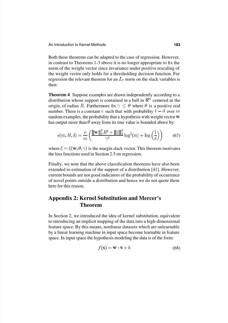
Both these theorems can be adapted to the case of regression. However,in contrast to Theorems 1-3 above it is no longer appropriate to fix the

norm of the weight vector since invariance under positive rescaling of

the weight vector only holds for a thresholding decision function. For

regression the relevant theorem for an

norm on the slack variables is

then:



centered at the

origin, of radius . Furthermore fix where is a positive real

number. There is a constant

such that with probability Æ

over

random examples, the probability that a hypothesis with weight vector

has output more than away from its true value is bounded above by:

Æ

Æ

(67)

where is the margin slack vector. This theorem motivates

the loss functions used in Section 2.5 on regression.

Finally, we note that the above classification theorems have also been

extended to estimation of the support of a distribution [41]. However,current bounds are not good indicators of the probability of occurrence

of novel points outside a distribution and hence we do not quote them

here for this reason.

Appendix 2: Kernel Substitution and Mercer’s

Theorem

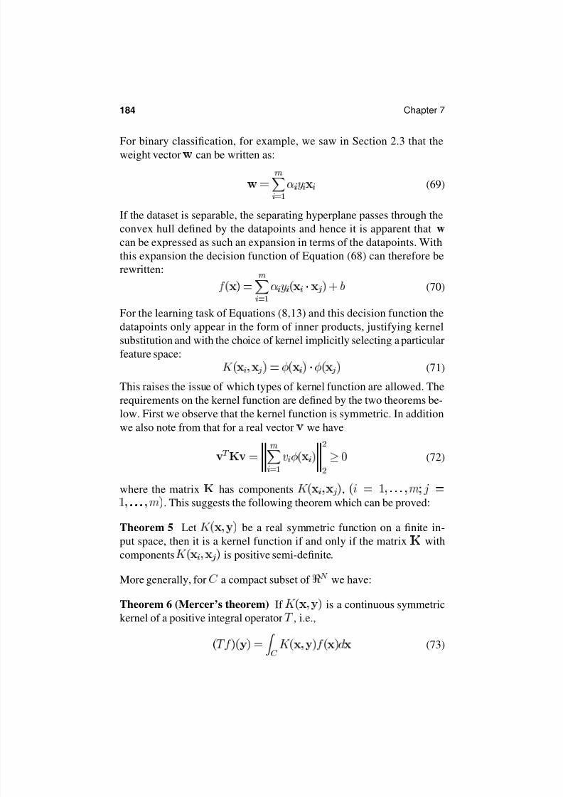
In Section 2, we introduced the idea of kernel substitution, equivalent

to introducing an implicit mapping of the data into a high-dimensional

feature space. By this means, nonlinear datasets which are unlearnableby a linear learning machine in input space become learnable in feature

space. In input space the hypothesis modeling the data is of the form:

(68)



184 Chapter 7

For binary classification, for example, we saw in Section 2.3 that theweight vector can be written as:

(69)

If the dataset is separable, the separating hyperplane passes through the

convex hull defined by the datapoints and hence it is apparent that w

can be expressed as such an expansion in terms of the datapoints. With

this expansion the decision function of Equation (68) can therefore be

rewritten:

(70)

For the learning task of Equations (8,13) and this decision function the

datapoints only appear in the form of inner products, justifying kernel

substitution and with the choice of kernel implicitly selecting a particular

feature space:

(71)

This raises the issue of which types of kernel function are allowed. The

requirements on the kernel function are defined by the two theorems be-

low. First we observe that the kernel function is symmetric. In additionwe also note from that for a real vector we have

(72)

where the matrix has components

,

. This suggests the following theorem which can be proved:

Theorem 5 Let

be a real symmetric function on a finite in-

put space, then it is a kernel function if and only if the matrix

with

components

is positive semi-definite.

More generally, for a compact subset of

we have:

Theorem 6 (Mercer’s theorem) If is a continuous symmetric

kernel of a positive integral operator , i.e.,

(73)




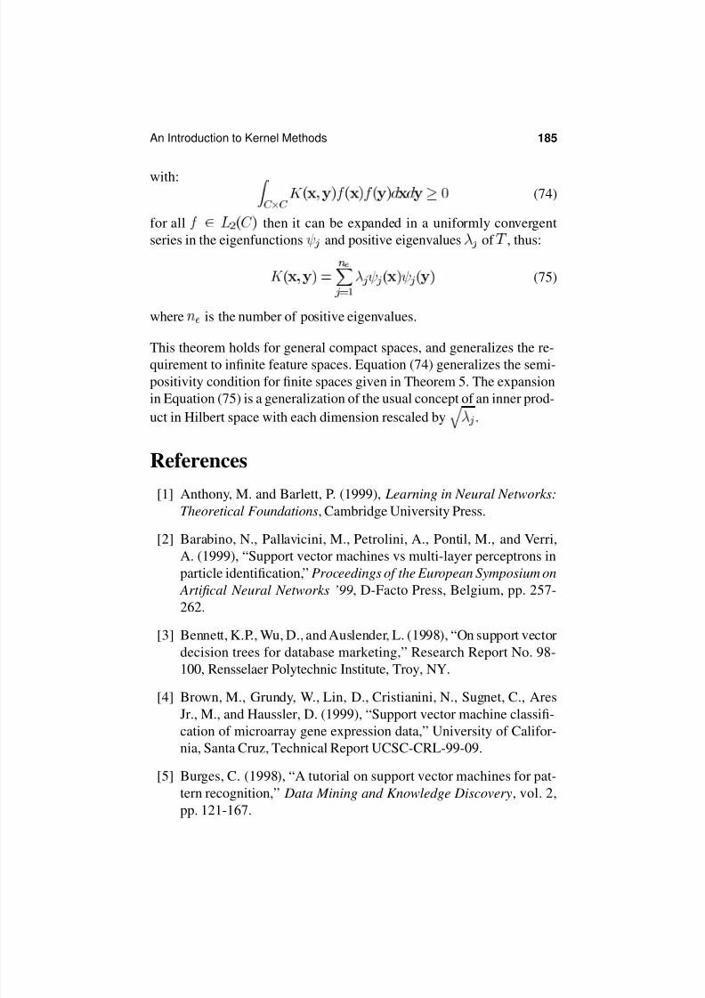
with:

(74)

for all

then it can be expanded in a uniformly convergent

series in the eigenfunctions

and positive eigenvalues

of

, thus:

(75)

where

is the number of positive eigenvalues.

This theorem holds for general compact spaces, and generalizes the re-quirement to infinite feature spaces. Equation (74) generalizes the semi-

positivity condition for finite spaces given in Theorem 5. The expansion

in Equation (75) is a generalization of the usual concept of an inner prod-

uct in Hilbert space with each dimension rescaled by

.

References

[1] Anthony, M. and Barlett, P. (1999), Learning in Neural Networks:

Theoretical Foundations, Cambridge University Press.

[2] Barabino, N., Pallavicini, M., Petrolini, A., Pontil, M., and Verri,

A. (1999), “Support vector machines vs multi-layer perceptrons in

particle identification,” Proceedings of the European Symposium on

Artifical Neural Networks ’99, D-Facto Press, Belgium, pp. 257-

262.

[3] Bennett, K.P., Wu, D., and Auslender, L. (1998), “On support vector

decision trees for database marketing,” Research Report No. 98-

100, Rensselaer Polytechnic Institute, Troy, NY.

[4] Brown, M., Grundy, W., Lin, D., Cristianini, N., Sugnet, C., AresJr., M., and Haussler, D. (1999), “Support vector machine classifi-

cation of microarray gene expression data,” University of Califor-

nia, Santa Cruz, Technical Report UCSC-CRL-99-09.

[5] Burges, C. (1998), “A tutorial on support vector machines for pat-

tern recognition,” Data Mining and Knowledge Discovery, vol. 2,

pp. 121-167.



186 Chapter 7

[6] Campbell, C., Cristianini, N., and Smola, A. (2000), “Instanceselection using support vector machines,” submitted to Machine

Learning.

[7] Chapelle, O. and Vapnik, V. (2000), “Model selection for support

vector machines,” in Solla, S.A., Leen, T.K., and Muller, K.-R.

(Eds.), Advances in Neural Information Processing Systems, vol.

12, MIT Press. To appear.

[8] Cortes, C. and Vapnik, V. (1995), “Support vector networks,” Ma-

chine Learning, vol. 20, pp. 273-297.

[9] Cristianini, N., Campbell, C., and Shawe-Taylor, J. (1999), “Dy-

namically adapting kernels in support vector machines,” in Kearns,

M., Solla, S.A., and Cohn, D. (Eds.), Advances in Neural Informa-

tion Processing Systems, vol. 11, MIT Press, pp. 204-210.

[10] Cristainini, N. and Shawe-Taylor, J. (2000), An Introduction to Sup-

port Vector Machines and other Kernel-Based Learning Methods,

Cambridge University Press. To appear January.

[11] Drucker, H., Wu, D., and Vapnik, V. (1999), “Support vector ma-

chines for spam categorization,” IEEE Trans. on Neural Networks,vol. 10, pp. 1048-1054.

[12] Drucker, H., Burges, C., Kaufman, L., Smola, A., and Vapnik, V.

(1997), “Support vector regression machines,” in Mozer, M., Jor-

dan, M., and Petsche, T. (Eds.), Advances in Neural Information

Processing Systems, vol. 9, MIT Press, Cambridge, MA.

[13] Dumais, S., Platt, J., Heckerman, D., and Sahami, M. (1998), “In-

ductive learning algorithms and representations for text categoriza-

tion,” 7th International Conference on Information and Knowledge

Management .

[14] Fernandez, R. and Viennet, E. (1999), “Face identification using

support vector machines,” Proceedings of the European Symposium

on Artificial Neural Networks (ESANN99), D.-Facto Press, Brus-

sels, pp. 195-200.




[15] Friess, T.-T., Cristianini, N., and Campbell, C. (1998), “The kerneladatron algorithm: a fast and simple learning procedure for sup-

port vector machines,” 15th Intl. Conf. Machine Learning, Morgan

Kaufman Publishers, pp. 188-196.

[16] Guyon, I., Matic, N., and Vapnik, V. (1996), “Discovering infor-

mative patterns and data cleaning,” in Fayyad, U.M., Piatetsky-

Shapiro, G., Smyth, P., and Uthurusamy, R. (Eds.), Advances in

Knowledge Discovery and Data Mining, MIT Press, pp. 181-203.

[17] Cf.: http://www.clopinet.com/isabelle/Projects/SVM/applist.html .

[18] Haussler, D. (1999), “Convolution kernels on discrete structures,”

UC Santa Cruz Technical Report UCS-CRL-99-10.

[19] Herbrich, R., Graepel, T., and Campbell, C. (1999), “Bayesian

learning in reproducing kernel Hilbert spaces,” submitted to Ma-

chine Learning.

[20] Herbrich, R., Graeppel, T., and Bollmann-Sdorra, P. (2000), ”A

PAC-Bayesian study of linear classifiers: why SVMs work,”

preprint under preparation, Computer Science Department, TU,

Berlin.

[21] Jaakkola, T., Diekhans, M., and Haussler, D. (1999), “A discrim-

inative framework for detecting remote protein homologies,” MIT

preprint.

[22] Jaakkola, T. and Haussler, D. (1999), “Probabilistic kernel regres-

sion models,” Proceedings of the 1999 Conference on AI and Statis-

tics.

[23] Joachims, T. (1998), “Text categorization with support vector ma-

chines: learning with many relevant features,” Proc. European Con- ference on Machine Learning (ECML).

[24] Keerthi, S., Shevade, S., Bhattacharyya, C., and Murthy, K. (1999),

“Improvements to Platt’s SMO algorithm for SVM classifier de-

sign,” Tech. Report, Dept. of CSA, Banglore, India.



188 Chapter 7

[25] Kwok, J. (1999), “Moderating the outputs of support vector ma-chine classifiers,” IEEE Transactions on Neural Networks, vol. 10,

pp. 1018-1031.

[26] Kwok, J. (1999), “Integrating the evidence framework and support

vector machines,” Proceedings of the European Symposium on Ar-

tificial Neural Networks (ESANN99), D.-Facto Press, Brussels, pp.

177-182.

[27] Luenberger, D. (1984), Linear and Nonlinear Programming,

Addison-Wesley.

[28] Mayoraz, E. and Alpaydin, E. (1999), “Support vector machines for

multiclass classification,” Proceedings of the International Work-

shop on Artifical Neural Networks (IWANN99), IDIAP Technical

Report 98-06.

[29] Mika, S., Ratsch, G., Weston, J., Scholkopf, B., and Muller, K.-R.

(1999), “Fisher discriminant analysis with kernels,” Proceedings of

IEEE Neural Networks for Signal Processing Workshop.

[30] Olivetti Research Laboratory (1994), ORL dataset , http://www.orl.

co.uk/facedatabase.html .

[31] Osuna, E. and Girosi, F. (1999) “Reducing the run-time complex-

ity in support vector machines,” in Scholkopf, B., Burges, C., and

Smola, A. (Eds.), Advances in Kernel Methods: Support Vector

Learning, MIT press, Cambridge, MA, pp. 271-284.

[32] Osuna, E., Freund, R., and Girosi, F. (1997) “Training support

vector machines: an application to face detection,” Proceedings of

CVPR’97 , Puerto Rico.

[33] Platt, J. (1999), “Fast training of SVMs using sequential minimal

optimization,” in Scholkopf, B., Burges, C., and Smola, A. (Eds.), Advances in Kernel Methods: Support Vector Learning, MIT press,

Cambridge, MA, pp. 185-208.

[34] Platt, J., Cristianini, N., and Shawe-Taylor, J. (2000), “Large margin

DAGS for multiclass classification,” in Solla, S.A., Leen, T.K., and

Muller, K.-R. (Eds.), Advances in Neural Information Processing

Systems, 12 ed., MIT Press.




[35] Papageorgiou, C., Oren, M., and Poggio, T. (1998), “A generalframework for object detection,” Proceedings of International Con-

ference on Computer Vision, pp. 555-562.

[36] Roobaert, D. (1999), “Improving the generalization of linear sup-

port vector machines: an application to 3D object recognition with

cluttered background,” Proc. Workshop on Support Vector Ma-

chines at the 16th International Joint Conference on Artificial In-

telligence, July 31-August 6, Stockholm, Sweden, pp. 29-33.

[37] Rychetsky, M., Ortmann, S., and Glesner, M. (1999), “Support vec-

tor approaches for engine knock detection,” Proc. International Joint Conference on Neural Networks (IJCNN 99), July, Washing-

ton, U.S.A.

[38] Scholkopf, B., Bartlett, P., Smola, A., and Williamson, R. (1998),

“Support vector regression with automatic accuracy control,” in

Niklasson, L., Boden, M., and Ziemke, T. (Eds.), Proceedings of the

8th International Conference on Artificial Neural Networks, Per-

spectives in Neural Computing, Berlin, Springer Verlag.

[39] Scholkopf, B., Bartlett, P., Smola, A., and Williamson, R. (1999),

“Shrinking the tube: a new support vector regression algorithm,” in

Kearns, M.S., Solla, S.A., and Cohn, D.A. (Eds.), Advances in Neu-

ral Information Processing Systems, 11, MIT Press, Cambridge,

MA.

[40] Scholkopf, B., Burges, C., and Smola, A. (1998), Advances in Ker-

nel Methods: Support Vector Machines, MIT Press, Cambridge,

MA.

[41] Scholkopf, B., Platt, J.C., Shawe-Taylor, J., Smola, A.J., and

Williamson, R.C. (1999), “Estimating the support of a high-

dimensional distribution,” Microsoft Research Corporation Tech-

nical Report MSR-TR-99-87.

[42] Scholkopf, B., Shawe-Taylor, J., Smola, A., and Williamson, R.

(1999), “Kernel-dependent support vector error bounds,” Ninth In-

ternational Conference on Artificial Neural Networks, IEE Confer-

ence Publications No. 470, pp. 304-309.



190 Chapter 7

[43] Scholkopf, B., Smola, A., and Muller, K.-R. (1999), “Kernel princi-pal component analysis,” in Scholkopf, B., Burges, C., and Smola,

A. (Eds.), Advances in Kernel Methods: Support Vector Learning,

MIT Press, Cambridge, MA, pp. 327-352.

[44] Scholkopf, B., Smola, A., Williamson, R.C., and Bartlett, P.L.

(1999), “New support vector algorithms,” Neural Computation.

[45] Scholkopf, B., Sung, K., Burges, C., Girosi, F., Niyogi, P., Poggio,

T., and Vapnik, V. (1997), “Comparing support vector machines

with Gaussian kernels to radial basis function classifiers,” IEEE

Transactions on Signal Processing, vol. 45, pp. 2758-2765.

[46] Shawe-Taylor, J. (1997), “Confidence estimates of classification ac-

curacy on new examples,” in Ben-David, S. (Ed.), EuroCOLT97,

Lecture Notes in Artificial Intelligence, vol. 1208, pp. 260-271.

[47] Shawe-Taylor, J., Bartlett, P.L., Williamson, R.C., and Anthony,

M. (1998), “Structural risk minimization over data-dependent hi-

erarchies,” IEEE Transactions on Information Theory, vol. 44, pp.

1926-1940.

[48] Shawe-Taylor, J. and Cristianini, N. (1999), “Margin distributionand soft margin,” in Smola, A., Barlett, P., Scholkopf, B., and Schu-

urmans, C. (Eds.), Advances in Large Margin Classifiers, Chapter

2, MIT Press.

[49] Smola, A. and Scholkopf, B. (1998), “A tutorial on support vector

regression,” Tech. Report, NeuroColt2 TR 1998-03.

[50] Smola, A. and Scholkopf, B. (1997), “From regularization oper-

ators to support vector kernels,” in Mozer, M., Jordan, M., and

Petsche, T. (Eds), Advances in Neural Information Processing Sys-

tems, 9, MIT Press, Cambridge, MA.

[51] Smola, A., Scholkopf, B., and Muller, K.-R. (1998), “The connec-

tion between regularization operators and support vector kernels,”

Neural Networks, vol. 11, pp. 637-649.




[52] Smola, A., Williamson, R.C., Mika, S., and Scholkopf, B. (1999),“Regularized principal manifolds,” Computational Learning The-

ory: 4th European Conference, volume 1572 of Lecture Notes in

Artificial Intelligence, Springer, pp. 214-229.

[53] Sollich, P. (2000), “Probabilistic methods for support vector ma-

chines,” in Solla, S., Leen, T., and Muller, K.-R. (Eds.), Advances

in Neural Information Processing Systems, 12, MIT Press, Cam-

bridge, MA. (To appear.)

[54] Tax, D. and Duin, R. (1999), “Data domain description by sup-

port vectors,” in Verleysen, M. (Ed.), Proceedings of ESANN99, D.Facto Press, Brussels, pp. 251-256.

[55] Tax, D., Ypma, A., and Duin, R. (1999), “Support vector data de-

scription applied to machine vibration analysis,” in Boasson, M.,

Kaandorp, J., Tonino, J., Vosselman, M. (Eds.), Proc. 5th Annual

Conference of the Advanced School for Computing and Imaging,

Heijen, NL, June 15-17, pp. 398-405.

[56] Tipping, M. (2000), “The relevance vector machine,” in Solla, S.,

Leen, T., and Muller, K.-R. (Eds.), Advances in Neural Information

Processing Systems, MIT Press, Cambridge, MA. (To appear.)

[57] http://www.ics.uci.edu/˜mlearn/MLRepository.html .

[58] Vapnik, V. (1995), The Nature of Statistical Learning Theory,

Springer, N.Y.

[59] Vapnik, V. (1998), Statistical Learning Theory, Wiley.

[60] Vapnik, V. and Chapelle, O. (1999), “Bounds on error expectation

for support vector machines,” submitted to Neural Computation.

[61] Veropoulos, K, Campbell, C., and Cristianini, N. (1999), “Control-

ling the sensitivity of support vector machines,” Proceedings of the

International Joint Conference on Artificial Intelligence (IJCAI),

Stockholm, Sweden.

[62] Vidyasagar, M. (1997), A Theory of Learning and Generalisation,

Springer-Verlag, Berlin.



192 Chapter 7

[63] Watkins, C. (1999), “Dynamic alignment kernels,” Technical Re-port, UL Royal Holloway, CSD-TR-98-11.

[64] Weston, J. and Watkins, C. (1999), “Multi-class support vector ma-

chines,” in Verleysen, M. (Ed.), Proceedings of ESANN99, D. Facto

Press, Brussels, pp. 219-224.

[65] Zien, A., Ratsch, G., Mika, S., Scholkopf, B., Lemmen, C., Smola,

A., Lengauer, T., and Muller, K.-R. (1999), “Engineering support

vector machine kernels that recognize translation initiation sites,”

presented at the German Conference on Bioinformatics.

Introduction to SVMs

Documents

Transcript of Introduction to SVMs