Introduction to SuperconductivityVladimir Eltsov

Aalto University, Finland

Cryocourse 2016

CONTENTS

• Basic experimental properties of superconductors– Zero resistivity – Meissner effect – Phase diagram – Heat capacity

• Phenomenological description of superconductivity– Thermodynamics – Phase coherence and supercurrents – London equation– Flux quantization – Energy gap and coherence length – Clean and dirty– Type I and type II superconductors – Abrikosov vortices

• Introduction to the BCS theory– Electron-electron attraction – The Cooper problem – Model Hamiltonian– Bogolubov transformation – Bogolubov quasiparticles – The gap equation– Non-uniform superconductors – Bogolubov–de Gennes equations

• Andreev reflection and Andreev bound states– Scattering at the NIS interface – Bound states in SNS, SIS junctions– CdGM states in vortex cores – Supercurrent with bound states

• Josephson effect– DC and AC effect – Shunted junction and washboard potential– SQUID – Quantum dynamics

QUANTUM MECHANICS AT A HUMAN SCALE

Superconductivity was the first discovered macroscopic quantumphenomenon, where a sizable fraction of particles of a macroscopic objectforms a coherent state, described by a quantum-mechanical wave function.

Applications:

• High magnetic fields

• Filtering of radio signals

• Ultra-sensitive magnetic/temperature and other sensors

• Metrology

• Ultra-low-noise amplifiers

• Quantum engineering

• Quantum information processing

DISCOVERY OF SUPERCONDUCTIVITY

Heike Kamerlingh Onnes

Liquefied helium in 1908.

Resistivity of metals when T→0 ?

Au, Pt: ρ(T ) = const

Res

ista

nce,

Ohm

Mercury sample, 1911

Temperature, K

BASIC EXPERIMENTAL PROPERTIES: Zero resistivity

ρn

ρ = 0

TTc

ρ

Below the transition temperature Tc, the resistivity drops to zero.

Latest measurements put bound ρ < 10−23� cm.

Really zero!

Dirty metals are good superconductors.

THE MEISSNER EFFECT

Walther Meissner

Robert Ochsenfeld

T > Tc T < Tc

B B

At T < Tc the magnetic field is expelled from the super-conductor even if the field was applied before reaching Tc.

PHASE DIAGRAM OF A SUPERCONDUCTOR

Superconductivity is destroyed by sufficiently strong electric currents or bythe magnetic field above the critical field Hc.

T

H

Tc

Hc(0)

superconductor

normal

1st order

2nd order

Hc(T )

Empirically the dependence of Hc on temperature is described reasonablywell by

Hc(T ) = Hc(0)[1− (T /Tc)2]

THERMODYNAMICS OF THE SUPERCONDUCTING TRANSITION

In the external field H = Hc N S

Fn(T ) = Fs(T )+ H2c (T )

8π

Entropy S = −∂F/∂T : Sn − Ss = −Hc4πdHc

dT.

Heat capacity C = T ∂S/∂T : Cn − Cs = − T4π

[Hcd2Hc

dT 2+(dHc

dT

)2].

The heat capacity jump at Tc: Cs(Tc)− Cn(Tc) = Tc

4π

(dHc

dT

)2

.

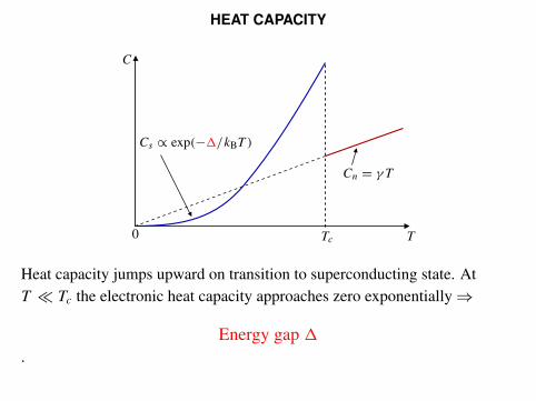
HEAT CAPACITY

TTc

Cn = γ T

Cs ∝ exp(−1/kBT )

0

C

Heat capacity jumps upward on transition to superconducting state. AtT � Tc the electronic heat capacity approaches zero exponentially⇒

Energy gap 1.

PHASE COHERENCE

Electrons form pairs, which are bosons andcondense to a single state, described by thewave function ψ with the macroscopicallycoherent phase χ .

ψ = |ψ | exp(iχ)

H⇒ js

Currentjs = e∗

2m∗[ψ∗pψ + ψ p†ψ∗

]

withp = −ih∇ − (e∗/c)A .

We get for e∗ = 2e, m∗ = 2m and the density of pairs |ψ |2 = ns/2:

js = −(e∗)2

m∗c|ψ |2

(A− hc

e∗∇χ

)= −e

2ns

mc

(A− hc

2e∇χ

).

THE LONDON EQUATION

Assuming density of superconducting electrons ns is constant:

js = −e2ns

mc

(A− hc

2e∇χ

)⇒ curl js = −e

2ns

mccurl A = −e

2ns

mch .

Fritz London

Heinz London

Using the Maxwell equation

js = (c/4π) curl h

we get the London equation

h+ λ2L curl curl h = 0 ,

where the London penetration depth

λL =(

mc2

4πnse2

)1/2

.

MEISSNER EFFECT

h+ λ2L curl curl h = 0 ⇒ h = λ2

L∇2h[curl curl h = ∇���div h−∇2h]

h

hy

x0

S

λL

∂2hy

∂x2− λ−2

L hy = 0

hy = hy(0) exp(−x/λL)

Magnetic field penetrates into a superconductor only over distances

λL =(

mc2

4πnse2

)1/2

Typical metal with m ∼ me and a0 ∼ 4 A, ns ∼ a−30 ⇒ λL ∼ 30 nm

MAGNETIC FLUX QUANTIZATION

Integrating expression

js = −e2ns

mc

(A− hc

2e∇χ

)

along a closed contour within a superconductor

−mce2

∮n−1s js · dl =

∫

S

curl A · dS− hc2e1χ = 8− hc

2e2πn

B

l

8 is the magnetic flux through the contour.

8′ = 8+ 4πc

∮λ2L js · dl = 80n

Quantum of magnetic flux

80 = πhc

|e| ≈ 2.07× 10−7 Oe · cm2 .

In SI units, 80 = πh/|e| = 2.07× 10−15T·m2.

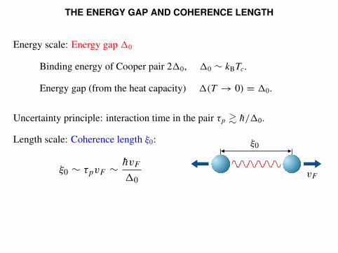
THE ENERGY GAP AND COHERENCE LENGTH

Energy scale: Energy gap 10

Binding energy of Cooper pair 210, 10 ∼ kBTc.

Energy gap (from the heat capacity) 1(T → 0) = 10.

Uncertainty principle: interaction time in the pair τp & h/10.

Length scale: Coherence length ξ0:

ξ0 ∼ τpvF ∼ hvF

10

ξ0

vF

COHERENCE LENGTH AND THE CRITICAL FIELD

Maximum phase gradient (∇χ)max ∼ 1/ξ sets the maximum supercurrent

js = −e2ns

mc

(A− hc

2e∇χ

)⇒ (js)max ∼ hnse

m(∇χ)max

Maximum supercurrent is reached when screening the critical field Hc

(js)max ∼ (c/4π)Hc/λLCritical field

Hc ∼ 4πλLc

hnse

mξ= πhc

e

λL

πξ

4πnse2

mc2= 80

πξλL

Condensation energy [remember ξ0 ∼ hvF /10]

Fn(0)− Fs(0) = H 2c (0)8π

∼ n

2mv2F

120 ∼ [N(0)10]10

EF

∼10

N(0) ∼ n/EF — density of states, EF = mv2F /2 — Fermi energy

LONDON AND PIPPARD REGIMES

Two length scales: London penetration depth and coherence length.

How do their values compare?

Typical metallic superconductor [like Al] with Tc = 1 K, the electrondensity n one per ion, lattice constant a0 ∼ 4 A:

ns ≈ n = a−30 ≈ 4 · 1022 cm−3, vF = pF /m = (h/m)(3π2n)1/3 ≈ 108 cm/s

ξ0 = hvF

2πkBTc≈ 1400 nm � λL =

(mc2

4πnse2

)1/2

≈ 30 nm

ξ0 ξ0

H HλL

Pippard regime London regime

λL

T → Tc

ns → 0λL→∞

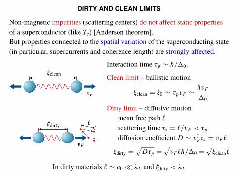
DIRTY AND CLEAN LIMITS

Non-magnetic impurities (scattering centers) do not affect static propertiesof a superconductor (like Tc) [Anderson theorem].But properties connected to the spatial variation of the superconducting state(in particular, supercurrents and coherence length) are strongly affected.

ξclean

ξdirty

vF

vF

ℓ

Interaction time τp ∼ h/10.

Clean limit – ballistic motion

ξclean = ξ0 ∼ τpvF ∼ hvF

10

Dirty limit – diffusive motionmean free path `scattering time τs = `/vF < τp

diffusion coefficient D ∼ v2F τs = vF `

ξdirty =√Dτp =

√vF `h/10 =

√ξclean`

In dirty materials ` ∼ a0 � λL and ξdirty < λL

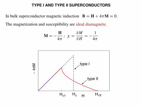
TYPE I AND TYPE II SUPERCONDUCTORS

In bulk superconductor magnetic induction B = H+ 4πM = 0.

The magnetization and susceptibility are ideal diamagnetic

M = − H4π; χ = ∂M

∂H= − 1

4π−

4πM

H Hc1 c2HHc

type I

type II

INTERMEDIATE STATE OF TYPE I SUPERCONDUCTORS

In the external field H < Hc the sample is divided to normal andsuperconducting domains so that in the normal phase magnetic inductionB = Hc while in the superconducting domains magnetic field is absent.

S NS

N NS S

B = H < Hc

B = 0

B = Hc

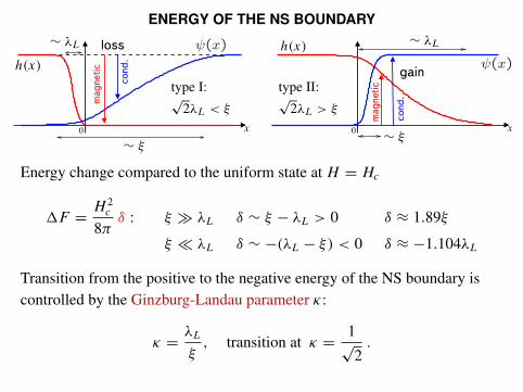
ENERGY OF THE NS BOUNDARY

x0x0

h(x)

h(x)

∼ ξ∼ ξ

∼ λL ∼ λL

type I:√2λL < ξ

type II:√2λL > ξ

ψ(x)

ψ(x)

mag

netic

mag

netic

cond

.

cond

.

loss

gain

Energy change compared to the uniform state at H = Hc

1F = H 2c

8πδ : ξ � λL δ ∼ ξ − λL > 0 δ ≈ 1.89ξ

ξ � λL δ ∼ −(λL − ξ) < 0 δ ≈ −1.104λL

Transition from the positive to the negative energy of the NS boundary iscontrolled by the Ginzburg-Landau parameter κ:

κ = λL

ξ, transition at κ = 1√

2.

THE GL PARAMETER FROM MATERIAL PARAMETERS

Order-parameter variation scale – coherence (healing) length ξ(T ) is not theCooper-pair size ξ0 (or ξdirty = √ξ0`):

ξ(T ) : gradient energy [ξ0]↔ condensation energy [T -dependent]

In the clean limit we have

ξ(T ) = ξ0

√7ζ(3)

12

[1− T

Tc

]−1/2

, λL = c

4|e|vF

√3

πN(0)

[1− T

Tc

]−1/2

κ = 3c|e|h

√π

7ζ(3)N(0)kBTc

v2F

= 3π2

√14ζ(3)

hc

e2

kBTc

EF

√e2/a0

EF∼ 103 kBTc

EF.

For usual superconductors kBTc/EF < 10−3 ⇒ κ . 1

For HTSC kBTc/EF ∼ 10−1 − 10−2 ⇒ κ � 1

For dirty superconductors with τs/τp � 1: κdirty ∼ κclean(τp/τs)� 1

ABRIKOSOV VORTICES

Magnetic field penetrates into type II superconductor in the form ofAbrikosov vortices, which are topologically-protected linear defects of theorder parameter: Order parameter is zero at the vortex axis and the phase ofthe order parameter winds by 2π on a loop around the vortex. Each vortexcarries a single quantum of magnetic flux 80.

Alexei Abrikosov

B

− 4π

M

H Hc1 c2HHc

nv – vortex density

80nv

ABRIKOSOV VORTICES

Magnetic field penetrates into type II superconductor in the form ofAbrikosov vortices, which are topologically-protected linear defects of theorder parameter: Order parameter is zero at the vortex axis and the phase ofthe order parameter winds by 2π on a loop around the vortex. Each vortexcarries a single quantum of magnetic flux 80.

Alexei Abrikosov

B

− 4π

M

H Hc1 c2HHc

nv – vortex density

80nv

ABRIKOSOV VORTEX STRUCTURE

00

1

20

5

1

10

2

15

3

r/ξ

r/λL

h(r)/Hc1

ψ(r)/ψeq

κ = 5

r∼

λL

r∼

ξ

r > λL: f = ψ(r)/ψeq = 1, h ∝ exp(−r/λL)ξ < r < λL: 1− f ∝ r−2, h ∝ ln(λL/r)

Main vortex energy here: Fv ≈ 820

16π2λ2L

ln κ

r < ξ (core): f ∝ r, h ≈ const

PHASE DIAGRAM OF TYPE-II SUPERCONDUCTORS

Meissner

VortexNormal

H

T T

HH

H

c

c

c1

c2

Hc1: vortex energetically favorable

Fv = (1/4π)80Hc1

Hc1 = 80

4πλ2L

ln κ = Hc ln κ√2κ

Hc: thermodynamic

Hc = 80

2√

2πλLξ

Hc2: no stable SC regions

Hc2 = 80

2πξ 2= Hc

√2κ

For ξ ∼ 2 nm one gets Hc2 ∼ 80 T.

RESISTIVITY FROM VORTEX MOTION

Lorentz force acting on vortex fromelectric current

fL = 80

c[jex × b] .

b

f

j

L

ex

Per unit volume we have

FL = nvfL = c−1[jex × (nv80b)] = c−1[jex × B] .

If vortex moves with friction η: vL = fL/η

E = c−1[B× vL] = (80B/ηc2)jex

and resistivityρ = E/j ex = 80B/ηc

2 .

Magnetic field applications require pinning!

The BCS Theory

John Bardeen Leon Cooper John Robert Schrieffer

Nikolai Bogolubov

EXCITATIONS IN LANDAU FERMI LIQUIDAt T = 0 states with p < pF , E < EF

are filled, others are empty.

n = p3F

3π2h3 , pF ∼ hn1/3 = h/a0

Fp

p−p’

p’

particlehole

(p /2m) −E2F

εp

0pp

F

particlesholes

εp ={

p2

2m − EF , p > pF

EF − p2

2m , p < pF

εp ≈ vF |p − pF |

f (εp) = 1eεp/kBT + 1

Constant density of states N(εp = 0) = N(p = pF ) = N(0) = m∗pF2π2h3 .

ELECTRON ATTRACTION: Polarization of the lattice

Atomic energy scale

Mω2Da

20 ∼

e2

a0∼ (h/a0)

2

m

Debye frequency

ωD ∼ EF

h

√m

M

Length of electron tail

∼ vFω−1D ∼

√M/ma0 ∼ 300a0 ⇒ p1 ≈ ±p2

p1

p1

p′1

p′1

p′2

p′2

p2

p2

EF ± hωD

⇒ p1 ≈ −p2

ELECTRON ATTRACTION: Model

p1 p′2

p1p′2

p′1 p2

p′1p2

−q q

(1) (2)

〈II|He−ph−e|I〉 = 2|Wq|2h

ωq

ω2 − ω2q< 0

attraction if ω < ωq ∼ ωD

Does not depend on the directions of p1, p2 ⇒ orbital momentum L = 0⇒ opposite spins

Model: Two electrons with opposite momenta and spins attract each otherwith the constant amplitude −W if εp1 < Ec and εp2 < Ec (whereEc ∼ hωD) and do not interact otherwise.

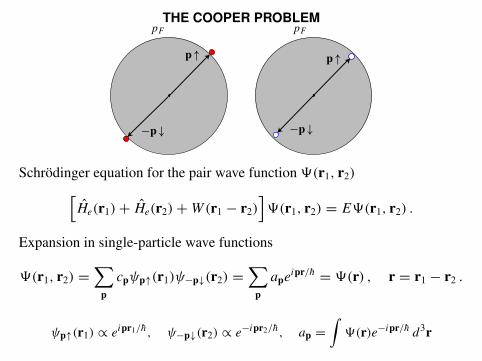
THE COOPER PROBLEMpF pF

p↑ p↑

−p↓ −p↓

Schrodinger equation for the pair wave function 9(r1, r2)

[He(r1)+ He(r2)+W(r1 − r2)

]9(r1, r2) = E9(r1, r2) .

Expansion in single-particle wave functions

9(r1, r2) =∑

p

cpψp↑(r1)ψ−p↓(r2) =∑

p

apeipr/h = 9(r) , r = r1 − r2 .

ψp↑(r1) ∝ eipr1/h, ψ−p↓(r2) ∝ e−ipr2/h, ap =∫9(r)e−ipr/h d3r

THE COOPER PROBLEM: Fourier transformed equation

Schrodinger equation becomes

2εpap +∑

p′Wp,p′ap′ = Eap .

Interaction model:

Wp,p′ =

−W, εp and εp′ < Ec,

i.e. pF − Ec/vF < p(and p′) < pF + Ec/vF0, otherwise

We thus have

ap = − W

E − 2εp

∑

p′,εp′<Ec

ap′ = − WC

E − 2εp

− 1W=

∑

p,εp<Ec

1E − 2εp

≡ 8(E)

E

8(E)

2ǫ0

2ǫn

−W−1

Eb

THE COOPER PROBLEM: Bound state

Bound state with E = Eb < 0

1W=

∑

p,εp<Ec

12εp − Eb .

Sum over momentum→ the integral over energy:

1W= 2N(0)

∫ Ec

0

dεp

2εp + |Eb| = N(0) ln( |Eb| + 2Ec|Eb|

).

From this equation we obtain

|Eb| = 2Ece1/N(0)W − 1

For weak coupling, N(0)W � 1, we find

|Eb| = 2Ece−1/N(0)W

For strong coupling, N(0)W � 1,

|Eb| = 2N(0)WEc

THE BCS MODEL: Non-interacting Hamiltonian

Non-interacting particles at k > kF and holes at k < kF

H0 =∑

kσ,k>kF

εkc†kσ ckσ +

∑

kσ,k<kF

εkh†kσhkσ .

But h†kσ = c−k,−σ and hkσ = c†

−k,−σ and we have

kF

k

ǫk

ξk

H0 =∑

kσ,k>kF

εkc†kσ ckσ +

∑

kσ,k<kF

ε−kckσ c†kσ

=∑

kσ,k>kF

εkc†kσ ckσ −

∑

kσ,k<kF

εkc†kσ ckσ +

∑

kσ,k<kF

εk =∑

kσ

ξkc†kσ ckσ + E0 .

Here we defined ckσ c†kσ = 1− c†

kσ ckσ

ξk = sign(k − kF )εk = h2k2

2m− EF ≈ hvF (k − kF ) .

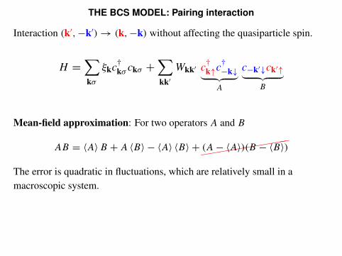
THE BCS MODEL: Pairing interaction

Interaction (k′,−k′)→ (k,−k) without affecting the quasiparticle spin.

H =∑

kσ

ξkc†kσ ckσ +

∑

kk′Wkk′ c

†k↑c

†−k↓︸ ︷︷ ︸A

c−k′↓ck′↑︸ ︷︷ ︸B

Mean-field approximation: For two operators A and B

AB = 〈A〉B + A 〈B〉 − 〈A〉 〈B〉 +((((

((((((

(A− 〈A〉)(B − 〈B〉)

The error is quadratic in fluctuations, which are relatively small in amacroscopic system.

THE BCS MODEL: Hamiltonian

HBCS =∑

kσ

ξkc†kσ ckσ +

∑

k

(1∗kc−k↓ck↑ +1kc

†k↑c

†−k↓ −1k

⟨c

†k↑c

†−k↓

⟩)

We defined 1k =∑

k′Wkk′

⟨c−k′↓ck′↑

⟩, thus 1∗k =

∑

k′Wkk′

⟨c

†k′↑c

†−k′↓

⟩

We want to diagonalize it with Bogolubov transformation

HBCS =∑

kσ

Ekγ†kσγkσ + Econd

Here γ †kσ and γkσ are new Bogolubov quasiparticles with spectrum Ek.

New operators mix particles and holes:

γ†k↑ = uk c

†k↑ + vk h

†k↑

γ−k↓ = u∗k c−k↓ − v∗k h−k↓

h†k↑ = c−k↓h−k↓ = c†

k↑

{γkσ , γ

†k′σ ′

}= δkk′δσσ ′ , {γkσ , γk′σ ′} =

{γ

†kσ , γ

†k′σ ′

}= 0 ⇒ |uk|2+|vk|2 = 1

THE BCS MODEL: Diagonal form

The desired form is

HBCS =∑

kσ

Ekγ†kσγkσ + Econd

with

Ek =√ξ2

k + |1k|2and

|uk|2 = 12

(1+ ξk

Ek

)

|vk|2 = 12

(1− ξk

Ek

)

kFk0

1

Equal admixture of

particle and hole

uk2

k2v

BOGOLUBOV QUASIPARTICLES: Energy spectrum

E

p p

F

F

∆particlesholes

E

Ep =√ε2

p + |1|2

≈√v2F (p − pF )2 + |1|2

Landau criterion vc = min(Ep/p) ≈ |1|/pF

BOGOLUBOV QUASIPARTICLES: Group velocity

For a given energy E > |1| there are two possible values of ξk:

ξ±k = ±√E2 − |1|2 = hvF (k± − kF ) , k± = kF ± 1

hvF

√E2 − |1|2 .

ξ+k , k+ — particles, ξ−k , k− — holes

k−k kFF

∆particlesparticles holesholes

E

0

k+−k− k−−k+

vg = dE

dp= kh

dE

dk, vparticles

g = vF√E2 − |1|2E

k, vholesg = −vF

√E2 − |1|2E

k.

BOGOLUBOV QUASIPARTICLES: Density of states

Since Ek =√ε2

k + |1|2 we have

∑

k

→ N(0)∫dεk = N(0)

∫d

(√E2

k − |1|2)= N(0)

∫EkdEk√E2

k − |1|2.

The density of states in the superconductoris

Ns(E) =

0, E 6 |1|,N(0)

E√E2 − |1|2 , E > |1|.

N(0)

N

∆ E

s

SELF-CONSISTENCY EQUATION

We insert Bogolubov transformation [ckσ → γkσ → (uk, vk)→ (1k, Ek)]into the gap definition and obtain equation for 1k [remember also Ek(1k)]

1k =∑

k′Wkk′

⟨c−k′↓ck′↑

⟩ = −∑

k′Wkk′

1k′

2Ek′[1− 2f (Ek′)]

We used Fermi distribution⟨γ

†kσγkσ

⟩= f (Ek) , f (E) = 1

eE/kBT + 1.

For our model interaction k dependence is simple

Wkk′ ={−W, εk and εk′ < Ec

0, otherwise1k =

{1, Ek <

√E2c + |1|2 ≈ Ec

0, otherwise

With these substitutions the gap equation becomes

1 = W1∑

k,εk<Ec

1− 2f (Ek)

2Ek= 1W

2

∑

k,εk<Ec

1Ek(1)

tanhEk(1)

2kBT

It has a trivial solution 1 = 0 corresponding to the normal metal.

THE GAP EQUATION

0.2 0.4 0.6 0.8 1.0

0.2

0.4

0.6

0.8

1.0

T /Tc

0

|1|/1

0

1 = λ∫ Ec

|1|

dE√E2 − |1|2 tanh

E

2kBT

Interaction constant λ = N(0)Wλ ∼ 0.1− 0.3 in practical superconductors

10 = (π/γ )kBTc ≈ 1.76kBTc

kBTc = (2γ /π)Ece−1/λ ≈ 1.13Ece−1/λ

|1| ∝ (1− T/Tc)1/2−→

↗10 − |1| ∝ exp(−10/kBT )

HEAT CAPACITY

Only quasiparticles contribute to the entropy

S = −kB

∑

kσ

[(1− f (Ek)) ln(1− f (Ek))+ f (Ek) ln f (Ek)]

f (Ek) = 1eEk/kBT + 1

, Ek =√ξ2

k + |1k(T )|2

The heat capacityTc T

S

norm

al

supe

rcon

d.

C = −T dSdT= 2kB

∑

k

f (Ek)(1− f (Ek))

[E2

kT 2− 1

2Td|1k|2dT

]

For T � Tc we have E ≈ 1� kBT and f (E) ≈ e−E/kBT .

As a result

C = 2√

2πkBN(0)10

(10

kBT

)3/2

exp(− 10

kBT

).

NON-UNIFORM SUPERCONDUCTORS

Real-space quasiparticle creation and annihilation operators

9†(r, σ ) =∑

k

e−ikrc†kσ , 9(r, σ ) =

∑

k

eikrckσ

Non-interacting Hamiltonian corresponds to

H0 =∑

kσ

ξkc†kσ ckσ → H0 =

∑

σ

∫d3r9†(r, σ )He9(r, σ )

where the free particle Hamiltonian

ξk = h2k2

2m− EF → He = 1

2m

(−ih∇−e

cA)2 + U(r)− µ,

which accounts for the magnetic field through the vector potential A andincludes some non-magnetic potential U(r).

BCS THEORY IN COORDINATE SPACE

Non-interacting→ add interaction (9†9†99)→ mean-field theory

→ diagonalize with Bogolubov transformation

9(r ↑) =∑

k

[uk(r)γk↑ − v∗k(r)γ †

−k↓]

9†(r ↓) =∑

k

[u∗k(r)γ

†−k↓ + vk(r)γk↑

]

Here k can be any enumeration of states, not necessarily wave vector.[For uniform case uk(r) = uke

ikr and vk(r) = vkeikr]

+ completeness/orthogonality conditions on uk(r) and vk(r) from Fermicommutation relations for 9 and γ .

BOGOLUBOV – DE GENNES EQUATIONS

Diagonalization condition{

He uk(r) + 1(r) vk(r) = Ek uk(r)

1∗(r) uk(r) − H ∗e vk(r) = Ek vk(r)

He = 12m

(−ih∇ − e

cA)2 + U(r)− µ

Self-consistency equation

1(r) = W∑

k,εk<Ec

uk(r)v∗k(r)[1− 2f (Ek)]

+ completeness/orthogonality conditions on uk(r) and vk(r)

+Maxwell equations to connect current and field

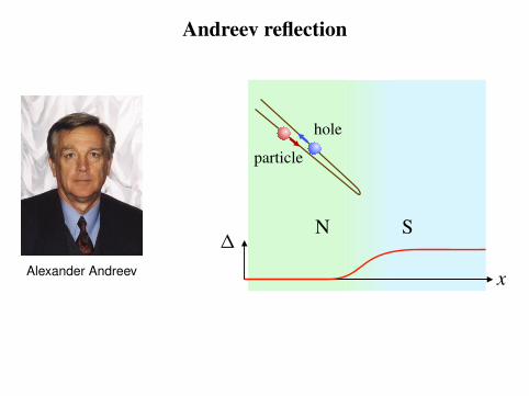
Andreev reflection

Alexander Andreev

1

x

N S

particle

hole

MODEL OF NS(NIS) INTERFACE

Bogolubov – de Gennes equations

− h2

2m

(∇ − ie

hcA)2

u(r)+ [Uex(r)− EF ] u(r)+1(r)v(r) = εu(r),

h2

2m

(∇ + ie

hcA)2

v(r)− [Uex(r)− EF ] v(r)+1∗(r)u(r) = εv(r).

Use uniform bulksolutions on leftand right

x

x

0

0

∆

N S

Uex

Uex(r) = Iδ(x)

Join(u, v, ∂xu, ∂xv)

at the interface

INCIDENT AND REFLECTED QUASIPARTICLES

Incident particle excitation with energy ε > |1|k±N = kF ± ε

hvF

k±S = kF ±√ε2 − |1|2hvF

Amplitudes (for I = 0)

a = A−/A+, b = 0c = 1/A+, d = 0

A± = 1√2

(1±

√ε2 − |1|2ε

)1/2

ki

ka

kb kc

kd

x

y

vga vgd

θ

kF kF−kF −kF

N

0

S

0

iab cd

ǫ ǫ

k+N k+S−k+N k−N −k−S

SUBGAP STATES

For an excitation coming from the normal side with ε < |1|Andreev reflection probability

|a|2 = |A−/A+|2 = 1 A± = 1√2

(1± i

√|1|2 − ε2

ε

)1/2

annihilated hole

penetrating particle incident particle

reflected hole

p

pp

p

vgCooper

pair

N S

-|e|

+|e|

-2|e|

vg

-2|e|

ANDREEV BOUND STATES

S SN

p

h

x0−d/2 d/2

1 = |1|eiφ/21 = |1|e−iφ/2

ǫ < |1|

Spectrum for short junction (d < ξ )

π0 2π

∆ǫ

φ

ppε = ∓|1| cos

φ

2

NEGATIVE ENERGIES

Bogolubov – de Gennes equations possess an important property: If(u(r)v(r)

)is a solution for the energy ε

then (v(r)∗

−u(r)∗)

is a solution for the energy − ε

Thus formally we can introduce negative energies and “Dirac sea” ofexcitations.

π0 2π

∆

−∆

kx < 0 kx > 0

ǫ

φ

SUPERCONDUCTOR–INSULATOR–SUPERCONDUCTOR (SIS) CONTACT

π π0 02 2π π

∆ ∆

− −∆ ∆

kx < 0 kx > 0

ǫ ǫ

φ φ21

√1 − T

No barrier, T = 1 Barrier, T < 1

ε = ±εφ = ±|1|√

1− T sin2(φ/2)

Conduction channel transmission coefficient T1RN= TR0, quantum of resistance R0 = πh

e2≈ 12.9 k�

BOUND FERMION STATES IN THE VORTEX CORE

Caroli, de Gennes, Matricon 1964

b x

y

y

x

particle

hole

a

a

Andreev reflection

εn(pz = 0, µ) ε0(pz, µ)1

−1

pz

n = 0

nmax

µ/pF

1

hω0

Radial quantum number n (nmax ∼ a/ξ ).

µ/h ={

m + 1/2, s-wave superconductors

m, superfluid 3He

Angular momentum µ = b p⊥, quantized.

Minigap ω0 ∼ 1

a pF∼ 1

h

12

EF≪ 1

h.

Anomalous (crossing zero) branch n = 0.

SUPERCURRENT VIA ANDREEV BOUND STATES

annihilated hole annihilated particle

penetrating particle penetrating particle bound state: particle

bound state: hole

p

pp

p

vg

Cooperpair

N SS

-|e|

+|e|

-2|e|-2|e|

vg

SUPERCURRENT IN THE POINT CONTACT

For the contact with resistance RN in the normal state supercurrent is

Is = π |1|sin(φ/2)eRN

tanh|1|cos(φ/2)

2kBT

0 π2π

φ

IT ≪ Tc

T → Tc

T � Tc : Is ≈ Icsin(φ/2) sign cos(φ/2)

Ic = π |1|eRN

T → Tc : Is ≈ Icsin(φ)

Ic = π |1|24kBT eRN

Josephson effect and weak links

Brian Josephson

|1|eiχ1 |1|eiχ2

φ = χ2 − χ1(φ)

DC Josephson effect AC Josephson effect

Is = Icsinφ hdφ

dt= 2eV

Ic is the critical Josephson current

WEAKLY COUPLED SUPERCONDUCTORS (Feynman model)

V

ϕ2 = −V/2

ϕ1 = V/2

Is

χ1 = −φ/2

χ2 = φ/2

Wave functions of the Cooper-pair condensateare uniform

ψ1 = N1/21 eiχ1, ψ2 = N1/2

2 eiχ2

N1, N2 – number of Cooper pairs.

When no coupling ψα = const (t)

ih∂ψα

∂t= Eαψα = 0 ⇒ Eα = 0, α = 1, 2

With coupling −K between the superconductors

ih∂ψ1

∂t= (E1 + e∗V/2)ψ1 −Kψ2

ih∂ψ2

∂t= (E2 − e∗V/2)ψ2 −Kψ1

Here e∗ = 2e is the charge of the Cooper pair.

DC JOSEPHSON EFFECT

We obtainhdN1

dt= −2K

√N1N2 sin(χ2 − χ1)

hdN2

dt= 2K

√N1N2 sin(χ2 − χ1)

This gives the charge conservation N1 +N2 = const together with therelation

Is = Icsinφ

whereIs = e∗ dN2

dt= −e∗ dN1

dt

is the current flowing from the first into the second electrode,

Ic = 4eK√N1N2/h

is the critical Josephson current, while φ = χ2 − χ1 is the phase difference.

AC JOSEPHSON EFFECT

For phases we find

hN2dχ2

dt= eVN2 +K

√N1N2 cos(χ2 − χ1)

hN1dχ1

dt= −eVN1 +K

√N1N2 cos(χ2 − χ1)

Subtracting we get

h(N2 −N1)d(χ2 − χ1)

dt= 2eV (N2 −N1)

or

hdφ

dt= 2eV

CAPACITIVELY AND RESISTIVELY SHUNTED JUNCTION

R J CI

I = C∂V∂t+ VR+ Ic sinφ, V = h

2e∂φ

∂t

I = hC

2e∂2φ

∂t2+ h

2eR∂φ

∂t+ Ic sinφ

Mechanical analogue: M∂2φ

∂t2= −η∂φ

∂t−∂U(φ)

∂φ

Particle with coordinate φ and with the “mass” M = h2C

4e2= h2

8EC

Medium with a viscosity η = h2

4e2R= h2

8ECRC, EC = e2

2C

Potential U(φ) = EJ (1− cosφ)− (hI/2e)φ = EJ (1− cosφ − φI/Ic)

EJ = hIc

2e

WASHBOARD POTENTIAL

U(φ) = EJ (1− cosφ − φI/Ic) , EJ = hIc

2eU

φ

Small oscillations around the minimum:

1− cosφ = 2 sin2(φ/2) ≈ φ2/2, U(φ) ≈ EJφ2

2

Plasma frequency Quality factor

ωp =√EJ

M=√

8EJECh

Q = ωpRC

EFFECTIVE INDUCTANCE

R J CI R L CI

|φ| � 2π ⇒ I ≈ Ic φ

V = h

2e∂φ

∂t≈ h

2eIc

∂IJ

∂tV = 1

c

∂8

∂t= L

c2

∂IL

∂t

The effective kinetic inductance of the Josephson junction

LJ = hc2

2eIcCritical current Ic depends e.g. on temperature ⇒ detectors.

Nonlinear inductance at large φ.

VOLTAGE BIAS

R JV

I

Let us consider the case when the constant voltageV is applied to the junction. In this case

∂φ

∂t= 2ehV = ωJ = const, φ = φ0 + ωJ t

Total currentI = V

R+ Ic sin(φ0 + ωJ t)

and the average current has simple ohmic behavior for any damping

I = V/R .

Thus for observation of non-trivial dynamics of Josephson junctions thecurrent bias is essential.

DYNAMICS OF JOSEPHSON JUNCTIONS

U

1

2φ

φ0

I < Ic

I < Ir

I > Ir

I > Ic

ω−2p

∂2φ

∂t2+Q−1ω−1

p

∂φ

∂t+ sinφ = I

IcLarge damping

Q−1ω−1p � ω−2

p ωJ ⇒ Q = RCωp � ωp/ωJ ⇒ RC � ω−1J

⇒ no inertia (capacitance)

Small damping ⇒ hysteretic behavior

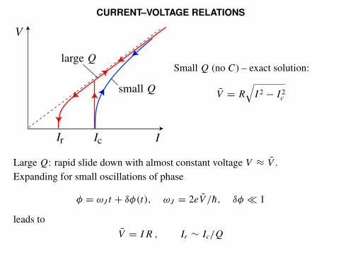
CURRENT–VOLTAGE RELATIONS

II

V

cIr

small Q

large QSmall Q (no C) – exact solution:

V = R√I 2 − I 2

c

Large Q: rapid slide down with almost constant voltage V ≈ V .Expanding for small oscillations of phase

φ = ωJ t + δφ(t), ωJ = 2eV /h, δφ � 1

leads toV = IR , Ir ∼ Ic/Q

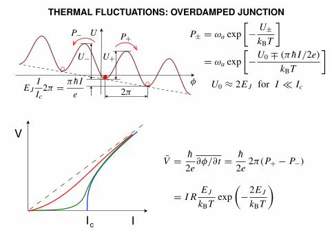
THERMAL FLUCTUATIONS: OVERDAMPED JUNCTION

U

φ

U+

P+P−

U−

2πEJ

I

Ic

2π = πhI

e

P± = ωa exp[− U±kBT

]

= ωa exp[−U0 ∓ (πhI/2e)

kBT

]

U0 ≈ 2EJ for I � Ic

II

V

c

V = h

2e∂φ/∂t = h

2e2π(P+ − P−)

= IR EJ

kBTexp

(−2EJkBT

)

SUPERCONDUCTING QUANTUM INTERFERENCE DEVICES

dc SQUID:

js = −e2ns

mc

(A− hc

2e∇χ

)= 0

χ3−χ1+χ2−χ4−2ehc

(∫ 3

1A · dl+

∫ 2

4A · dl

)= 0

(χ2 − χ1)︸ ︷︷ ︸φa

− (χ4 − χ3)︸ ︷︷ ︸φb

= 2ehc

∮

1342A · dl = 2π8

80

1

2

3

4Φ

Ib

I

Ia

Total current

I = Ia + Ib = Ic sinφa + Ic sinφb = 2Ic cos(π8

80

)sin(φa − π8

80

)

The maximum current depends on the magnetic flux through the loop

Ic,SQUID = 2∣∣∣∣Ic cos

(π8

80

)∣∣∣∣

INFLUENCE OF THE SQUID INDUCTANCE

Extra flux from the circulating current

Icirc = Ib − Ia2= Ic

2

[sin(φa − 2π8

80

)− sinφa

]

in the SQUID loop

8 = 8ext+LIcirc

c= 8ext−βL80

2πsin(π8

80

)cos

(φa − π8

80

)

Φ

Ib

I

I I

I

a circ

circ

Dimensionless parameter βL = 2eLIchc2

= L

LJ& 1 in practice

0.500

1.0 1.5 2.0 2.5 3.0

0.2

0.4

0.6

0.8

1.0

8ext/80

I c,S

QU

ID/2I

c

βL = 0

1

2

3

Together with

I = 2Ic cos(π8

80

)sin(φa − π8

80

)

determines maximum current

SHAPIRO STEPS

Microwave irradiation of the junction V = V0 + V1 cos(ωt) and

φ = 2eh

∫ t

0V (t ′) dt ′ = φ0 + ωJ t + a sin(ωt), ωJ = 2e

hV0, a = 2e

h

V1

ω

The supercurrent

I = Ic sinφ = Ic∞∑

n=−∞(−1)nJn(2eV1/hω) sin(φ0 + ωJ t − nωt)

When ωJ = nω, i.e. V0 = n(hω/2e)the supercurrent has a dc component In = IcJn(2eV1/hω) sin(φ0 + πn).

I

V

hω/2e

2hω/2e

3hω/2e

QUANTUM DYNAMICS OF JOSEPHSON JUNCTIONS

AnalogyJosephson junction↔ particle in the washboard potential

can be extended to quantum-mechanical description.If φ is the coordinate of the a particle, then the momentum operator is

pφ = −ih ∂∂φ

The Shrodinger equation for the wave function 9 is

H9 =[p2φ

2M+ U(φ)

]9 = E9

with

M = h2C

4e2= h2

8EC, U(φ) = EJ (1− cosφ)− (hI/2e)φ

Thus the Hamiltonian is

H = −4EC∂2

∂φ2+ EJ (1− cosφ − φI/Ic)

REQUIREMENTS FOR JUNCTION PARAMETERS

Kinetic energy↔ The charging energy of the capacitor

The operator of charge Q on the capacitor:

p2φ

2M= Q2

2C, Q = −2ie

∂

∂φ, [Q, φ]− = 2e

h[pφ, φ]− = −2ie

Quantum uncertainty in phase 1φ and in charge 1Q: 1φ1Q ∼ 2e.Effects for Q ∼ e are important:

EC = e2

2C� kBT , C = εA

4πd∼ 10 (100 nm)2

4π · 1 nm∼ 10−15 F ⇒ T � 1K

EC � h

1t= h

RC⇒ R �2h

e2∼ R0 = πh

e2

R

R C

S Sext

extC

V

L1 L2

Cext � C, R0 � Rext � R

SUPERCONDUCTING QUANTUM ELECTRONICS

Rapidly developing field. One of key players in quantum engineering andquantum information processing.

U

φ

qubits and

artificial atoms macroscopic quantum

tunnelling

CONCLUSIONS• Superconductivity is ubiquitous in conducting systems: metals, alloys,

dirty and disordered systems, organic materials, 2D system...

• Superconductivity originates in the Cooper pairing of conductioncarriers. In many systems the attractive interaction is mediated byphonons and pairing occurs in spin-singlet, orbital momentum zerostate. But more and more unconventional systems are being discovered.

• Besides zero resistivity, superconductors possess broad range ofinteresting and practically important properties: magnetic, thermal, etc.

• Nanotechnology opened a new world in studies and applications ofsuperconductors, in particular due to good matching to importantphysical length scales. In nanodevices Josephson effect and Andreevbounds states usually play key roles.

• Superconductors provide access to quantum-mechanical coherence atmacroscopic length scales: a base for revolutionizing the world withquantum technologies.

LITERATURE

M. Tinkham, Introduction to superconductivity. McGraw-Hill, New York. (1996); Dover Books (2004)

P. G. de Gennes, Superconductivity of metals and alloys.W. A. Benjamin, New York (1966); Perseus Books (1999)

A. A. Abrikosov, Fundamentals of the theory of metals.North Holland, Amsterdam (1998)