INTRODUCTION TO STATISTICAL NEURODYNAMICS: EFFECTS OF ADDITIVE AND PARAMETRIC NOISE

John Milton

Department of Neurology Committees on Neurobiology & Computational Neuroscience

The University of Chicago

In biology, an experimentalist typically repeats the same experiment several

times. The fact that the results obtained for each trial are never precisely the same leads to those published figures with “error bars” surrounding each data point that are familiar to all who read the scientific literature. What is the source of this variability? Of course some of the variability might be attributable to measurement error (Rabinovitch, 1995). However, with modern technology the uncertainty in making a measurement is typically much smaller than the observed trial-to-trial variability. Here we consider the possibility that this variability reflects the effects of uncontrolled perturbations on the dynamical system under study. These uncontrolled perturbations are referred to herein as “noise”.

The nervous system is continuously subjected to the effects of noise [Areili, et

al, 1996; Borsellino, et al, 1972; Cabrera and Milton, 2002; Hunter, et al, 2000; Stark, et al, 1958; Verveen and De Felice, 1974]. Historically, analysis of fluctuations of membrane current first attracted the attention of neurobiologists to the presence of ion channels, or pores, in neuronal membranes [Verveen and DeFelice, 1974]. Fluctuations in inter-spike intervals led to explorations of the nature of spike generating mechanisms [Tuckwell, 1989]. Just 50 years ago the concern was that noise might be detrimental to neural function [Calvin and Stevens, 1968; Fatt and Katz, 1950]. This worry was based on the fact that the root-mean-square voltage of the spontaneous fluctuations in membrane potential at a nerve ending with diameter 0.1 is of the order of 1 mV; a magnitude sufficient to affect the timing of neural spikes. However, since this time there has been the growing realization that noise plays essential roles in the sensory, motor and cognitive activities of the nervous system [Borsellino, et al, 1972; Cabrera and Milton, 2002; Cabrera, et al, 2004; Chance, et al, 2002; Douglas, et al, 1993; Eurich and Milton, 1996; Harris and Wolpert, 1998; Lindner, et al, 2004; Longtin, et al, 1990, 1991; Milton, et al, 2004; Milton and Mackey, 2000; Tuckwell, 1989]. Indeed, the addition of noise generated by an external noise generator into the nervous system can be used to therapeutic advantage [Moss and Milton, 2003; Priplata, et al, 2003]. Yet despite these observations few neurobiologists understand what noise is, how it is described, and the nature of its beneficial effects on neural function.

mµ

1

From a mathematical point of view there are only two ways that noise can affect the behavior of a dynamical system. First we can add noise to the solution of the equations that describe the time evolution of the stochastic dynamical system. This effect of noise is typically discussed under the heading “measurement noise” [Bendat and Piersol, 1986; Rabinovitch, 1995] and will only briefly be discussed here. Our attention is focused on the second possibility, namely that noise is part of the governing equations for the dynamical system. In this case noise plays an essential role in determining the solution of the stochastic differential equations. The noisy perturbations can either be added as a separate term to the governing equations (additive noise) or to the parameters (parametric noise). Our goal in these lectures is to discuss some effects of additive and parametric noise which have significant effects on neurodynamics. It is important to note that simulations using electronic analog circuits have played a major role in understanding the effects of noise on dynamical systems particularly when the governing equations are nonlinear [see, for example, Fauve and Heslot, 1983; Foss, et al, 1997; Gammaitoni, et al, 1998; Horowitz and Hill, 1993; Losson, et al, 1993; Sato, et al, 2000; Sinha and Moss, 1989; Yu and Lewis, 1989]. The outline of these lectures is as follows: First, we introduce the notion of a probability distribution and its associated probability density. Recent observations have emphasized that in many neurophysiological contexts the observed probability densities have much “fatter tails” that can be accounted for by a Gaussian probability density. Second, we introduce the study of the effects of additive noise by considering its effects on dynamical systems that have thresholds. The obvious application to neurodynamics arises in the description of the input-output relationships of spiking neurons. Finally, we examine the effects of parametric noise. Parametric noise is increasingly being recognized as having important roles, for example, in motor control. An interesting property of the effects of parametric noise in the vicinity of a threshold is the generation of probability densities with fat tails even in the case that the underlying dynamics are linear and deterministic! I. Random variables and their properties a). Introductory concepts Useful discussions of noise and random processes1 are Bailey [1964], Davenport and Root [1987], Evans, et al [1993], Gardiner [1990], Horsthemke and Lefever [1984], Jenkins and Watts [1968], Lasota and Mackey [1994], and MacDonald [1962].

Identify the outcome of each experiment as a point (possibly n-dimensional), s, in a sample space S. This sample space represents the 1 We restrict our attention to stationary stochastic processes, i.e. processes whose statistical properties, e.g. mean, standard deviation, do not change with time.

2

aggregate of all possible outcomes of the experiment. A random variable, x(s), defined on a sample space of points s will be called a random variable if for every real number A, a set of points s for which is one of the class of admissible sets for which the probability is defined. For example the sample space, S, for two coin flips isS H , where H indicates a head and T a tail. The random variable “number of heads” associates the number 0 with the set s , the number 1 with the set s H , and the number 2 with the set s . Of course we could choose other random variables, e.g. “number of tails”, “two heads”, “two tails”.

( )x s A≤

,T TH TT

1 =

{ , ,H H= }

} }}

} ]

)

)

)

{0 TT=

2 =

{ ,T TH

{HH

The probability P(A) that the outcome of a given experiment will be the event (A) can be expressed as the probability P that the sample point s, corresponding to the outcome of the experiment, falls in the subset of sample points S corresponding to the event A:

A(S )

A

P( A AA) P(s S ) P(S )= ∈ =where the notation s means that a point s is an element of the point set S . AS∈ A

A random variable may be discrete or continuous. A discrete random

variable x takes on only a finite number of values on a finite interval (Figure 1). Figure 1b shows an example of a discrete random variable that takes on only five possible values, { on the interval [ . The probability

associated with each is P . The function of X whose value is the

probability that random variable x is less than or equal to X is called the probability distribution function

1 2 3 4 5x ,x ,x ,x ,x

jx ( )jx

)X

,−∞ +∞

(P x ≤

P x (1) ( ) (

j

jX X

X P x≤

≤ = ∑ From Figure 1a we see that P x is a staircase function that is non-decreasing and is bounded between 0 and 1. It is perhaps easier to think of

as the cumulative probability function as X goes from left to right; however, this terminology is currently regarded as being redundant.

( X≤

(P x X≤

3

Figure 1: Probability distribution (top) for a discrete random variable that takes on only five values (bottom).

In general any random variable may be thought of as having both a

discrete and a continuous part. This is not surprising since even a continuous function can be represented as a staircase function with very closely spaced steps. However, in experimental situations we most often encounter the situation that the probability distribution is not only continuous but also differentiable with a continuous derivative, except, perhaps, at a discrete set of points. In this case more direct methods of analysis are possible since we can define a probability density function, p(x), as

(( ) dP x Xp XdX≤

=) (2)

where p(x) satisfies

(3) ( ) 1p x dx+∞

−∞

=∫ The above condition is the continuous random variable expression of the fact that the probability of a certain event is unity.

4

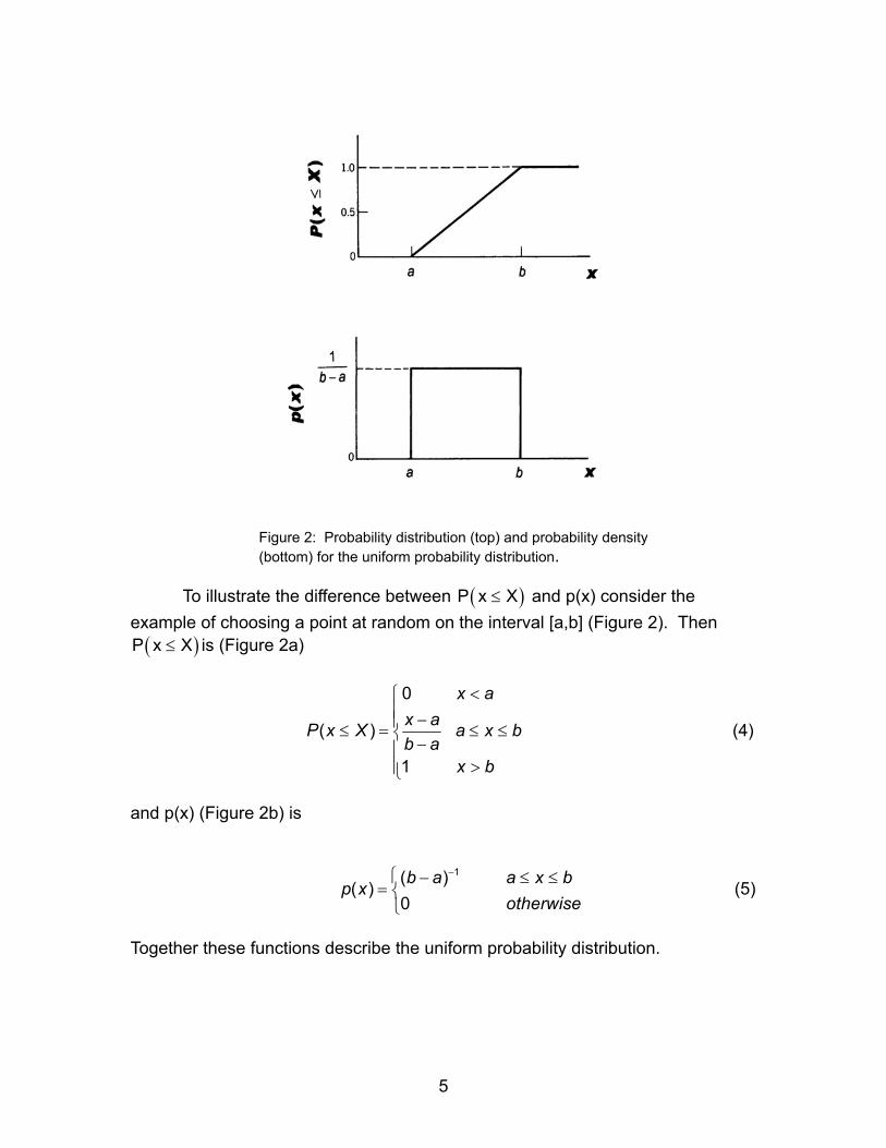
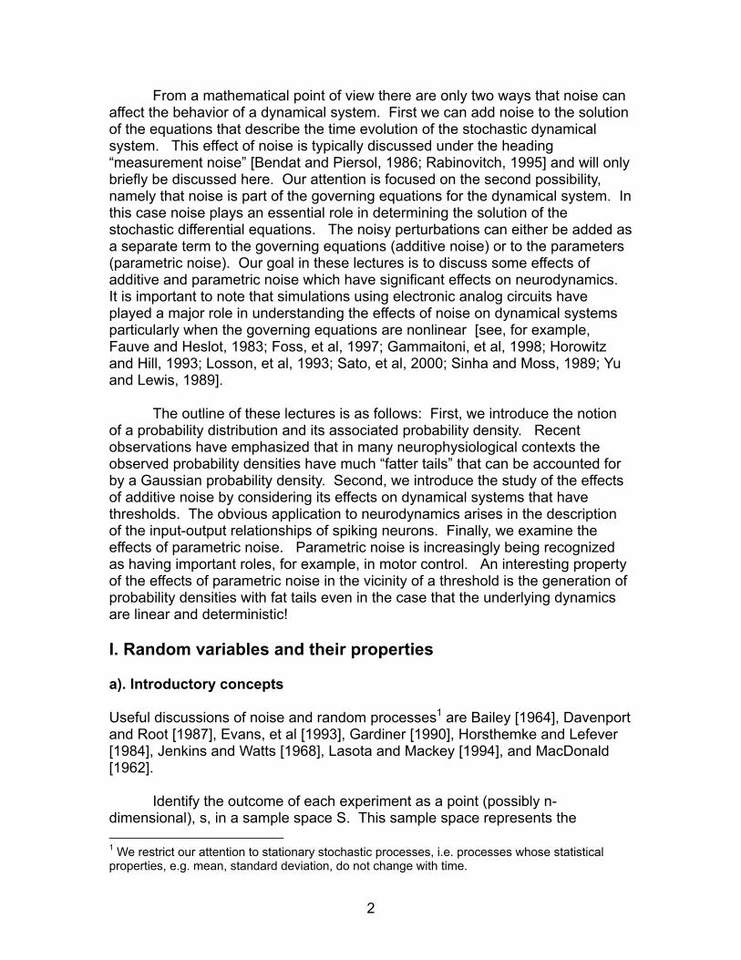
Figure 2: Probability distribution (top) and probability density (bottom) for the uniform probability distribution.

To illustrate the difference between P x and p(x) consider the

example of choosing a point at random on the interval [a,b] (Figure 2). Then is (Figure 2a)

( X≤ )

)(P x X≤

0

( )

1

x ax aX a x bb a

x b

< −≤ = ≤ ≤ −

>

P x (4)

and p(x) (Figure 2b) is

(5) 1( )( )

0b a a x bp x

otherwise

− − ≤=

≤

Together these functions describe the uniform probability distribution.

5

The probability that a continuous random variable has a value falling in the interval is given by the integral of the probability density function over that interval2

( < ≤a x b)

) (6) ( ) (< ≤ = ∫

b

aP a x b p x dx

From this relation we see that the probability that a continuous random variable takes on any specific value is zero. In other words, in a random dynamical system we cannot predict specific outcomes but rather only “an average” outcome following the performance of a very large number of experiments. Herein is the Achilles heel for the study of stochastic dynamical systems. We must be prepared to either perform a large number of experiments or a large number of numerical simulations in order to identify the behavior “on average”. The importance of the above defined probability functions, in particular p(x), is that they describe the long-run behavior of random variables. b). Moments

The various averages of random variables (e.g. the mean, variance, etc) measured experimentally can be determined from the probability density function, p(x). One group of averaged properties that are of considerable significance are the moments of p(x). The n-th moment of p(x) is the statistical average of the n-th power of x, i.e.

E x (7) ( ) ( )n nx p x dx+∞

−∞= ∫

For a stationary random process the first moment gives the mean or DC-component of the process. The second central moment gives the intensity of the varying component of the random process, i.e. the AC component. The positive square root of the variance is the standard deviation which is typically referred to as the root-mean-square (rms) value of the AC component of the random process.

For example the mean of the uniform distribution is

2 21 ( )( )

2 2

b

a

x b axp x dx dxb a b a

+∞

−∞

−= = = ⋅ =

− −∫ ∫b a+

µ (8)

and the variance is

2 Note that rather than is because we must exclude the case a (see below).

a x b< ≤ a x b≤ ≤ b=

6

2

2 2 (( ) ( )12

b ax p x dx+∞

−∞

−= − =∫

)σ µ (9)

Another averaged quantity that is of considerable importance is the

characteristic, or moment generating, function, which is the statistical average of exp( )ivx

M i (10) ( ) exp( ) ( )x v ivx p x dx+∞

−∞

= ∫ where v is real and 1= −i . Since p(x) is nonnegative and exp(ivx) has unit magnitude,

exp( ) ( ) ( ) 1ivx p x dx p x dx+∞ +∞

−∞ −∞

≤∫ ∫ = (11)

and hence the characteristic function always exists. It follows from the definition of the Fourier integral3 that the characteristic function of the probability distribution of a random variable x is the Fourier transform of the probability density function of that random variable [Bracewell, 1986; Brigham, 1988; Davenport and Root, 1987]. Therefore we may use the inverse Fourier transformation

1( ) ( )exp( )2 xp x M iv ivx dvπ

+∞

−∞

= ∫ −

(12)

to obtain the probability density function of a random variable when we know its characteristic function. It is often easier to determine the characteristic function first and then transform it to obtain the probability density than it is to determine the probability density directly (see below). c). Characterization of noise The specification of a set of experiments with the corresponding probability functions and random variables defines a random, or stochastic, process. Experimentally we measure three attributes to characterize the stochastic

3 The Fourier integral is defined as

H( i2 ftf ) h(t)e dtπ∞

−

−∞

= ∫If the integral exists for every value of the parameter f then H(f) is the Fourier transform of h(t).

7

process that generates the noisy inputs: 1) intensity; 2) probability density distribution; and 3) correlation time. i). Intensity: The intensity of noise is given by its variance. However, engineers and scientists typically refer to the intensity of noise in terms of its root-mean-square value which is equivalent to its standard deviation. It is important to note that whereas the variance of two independent noise signals is the sum of their variances, the rms value is not equal to the sum of the rms values, but is equal to 2 2

rms rms rmsa b) V (a) V (b)+ = +V ( . (13) ii). Correlation time: The correlation time t of a stationary stochastic process with density p(x) is defined by [Bendat and Piersol, 1986]

cor

cor0

1 CC(0)

∞

= ∫t (14) ( )dτ τ

0

where is the autocorrelation function of the noise process4 and C(0) is the variance. The rate at which goes to zero as is a measure of the memory time of the stochastic process. A process has short memory if

decays rapidly in relation to the characteristic relaxation time5 of the system, . The relaxation time of a system is estimated from its response to a brief

perturbation. In the case of the dynamical system we have .

C( )τ

1−

C( )τ τ → ∞

x(t)

C( )τsyst

sys =kx(t) 0+ =

t k All real noise is colored, i.e. is finite. In this lecture we restrict our attention to “white noise”, i.e. the special case for which . For white noise

is a Dirac delta function, hence white noise is often referred to as δ - correlated noise. The fact that the power spectrum of a white noise process is constant implies infinite power. Thus white noise is not physically realistic. However, it is found that white noise describes real noise surprisingly well when . The use of the white noise approximation greatly facilitates the mathematical analyses of noisy dynamical systems.

cort

cort =C( )τ

cor syst t

4 The autocorrelation function, , for a random process is R( )τ

T

0

1( ) lim y(t)y(t )dtT

τ τ∞

→∞= +∫R

5 The relaxation time of a system is estimated from its response to a brief perturbation. In the case of the dynamical system we have and is thus the time for the perturbation to decay to e-1 of its initial value.

x(t) kx(t) 0+ = 1syst k−=

8

iii). Probability density distribution function: Inspired largely by work in econophysics [Mantegna and Stanley, 1995; Stanley, et al, 1996], several studies have shown that fluctuations in physiological variables [Stanley, et al, 1998] ranging from the inter-beat interval of the heartbeat [Peng, et al, 1993] to movements of the fingertip during stick balancing [Cabrera and Milton, 2003, 2004b; Cabrera, et al, 2004] to the the interburst intervals of cultured neurons [Segev, et al, 2002] are described by p(x) having “fat tails”, i.e. distribution tails that are broader than can be readily explained by the Gaussian (normal) distribution.

Figure 3: Examples of the probability density functions for Lévy-stable distributions as a function of the Lévy index, α .

At first glance these observations are quite disturbing. The Central Limit Theorem states that the limit of normalized sums of independent identically distributed terms with finite variance must be Gaussian. The solution to this paradox is provided by relaxing the requirement that the variance is finite. The Generalized Central Limit Theorem states that the only possible nontrivial limits of normalized sums of independent identically distributed terms are Lévy-stable. All Lévy-stable, or stable, distributions have the property that if x and y are random variables from this family, then the random variable formed by x + y also has a distribution from this family. The Gaussian distribution is the only Lévy-stable distribution that has finite variance. As better measuring devices and larger data sets have become available it is being recognized that non-Gaussian Lévy distributions are prevalent in nature [Tsallis, et al, 1995].

α −

9

Lévy-stable distributions represent an example of a situation in which the

characteristic function is particularly useful. The characteristic function, M(z), for the symmetric Lévy distributions is (Woyczynski, 2001)

( ) 1( ) exp ' 1t z ixz dxM z e t ex

αγ

αγ

∞−

+−∞

= = −

∫

2

(15)

The parameter 0 is an index of the peakedness of a distribution, and the parameter γ ≥ is a scale factor that must be nonnegative. Note that the mean of the distribution, µ , exists only if 1 .

< α ≤0

2< α ≤

A characteristic feature of Lévy-stable distributions is that for asymptotically large displacements there is a power law decay of its density (16) ( )p x x β−≈where . 1β α= +

A practical difficulty in working with Lévy-stable distributions is that closed form expressions for p(x) exist only for three special certain choices of the parameters (Figure 3). For example the Gaussian distribution corresponds to the Lévy distribution withα = , γ = and µ =mean; the Cauchy distribution corresponds to the caseα = ; and the Lévy distribution (a confusing choice of terms) to the caseα = . However, since all of the Lévy-stable distributions are real-valued and symmetric about the mean (i.e. they are even functions), it follows that the Fourier transform and its inverse are real-valued functions. Thus the development of the Fast Fourier Transform and fast computers has enabled investigators to readily study models based on Lévy-stable models.

2,

0.5

2 / 2σ1

There are also a number of experimental challenges that arise in the

measurement of fluctuations described by the non-Gaussian variants of the Lévy-stable distribution. From a practical point of view probability densities with tails fatter than Gaussian means that events that are many times the standard deviation occur more frequently than for a Gaussian distributed variable. However, despite the increased frequency of these events they are still rare! Consequently very large data sets must be collected in order to ensure that these rare events are detected, e.g. ≥ data points [Weron, 2001]. In collecting time series these rare events can be missed unless proper attention is given to the choice of the frequency cut-offs of the low-pass and high-pass filters. Moreover it is crucially important that the sampling frequency is sufficiently high. It can be shown that as the sampling frequency decreases the distribution of the fluctuations necessarily must approach Gaussian [Mantegna and Stanley, 1995].

610

10

Recent excitement concerning Lévy phenomena in neurobiology stems from the relationship between a Lévy flight and a Lévy-stable distribution. A Lévy flight is a type of random walk that historically arose in the description of anomalous diffusion. It can be shown that after many steps the probability density of the displacement of a Lévy flight converges to a Lévy stable distribution. Surprisingly measurements of the foraging movements of animals and birds [Viswanathan, et al, 1996], eye movements during reading (Brockman and Geisel, 2000] and finger movements during stick balancing at the fingertip [Cabrera and Milton, 2004b] all are characterized by Lévy distributions with α ≤ . Lévy flights with this index are typical for super-diffusion [Brockman and Geisel, 2003; Rangarajan and Ding, 2000]. In particular it has been shown that Lévy flights with α ≈ are optimal for random search patterns [Brockman and Geisel, 2003; Buldyrev, et al, 2001, Viswanathan, et al, 1999].

1

1

II. Additive noise The paradigm for the effects of additive noise on the fluctuations of a fixed-point is the Langevin equation6

0( ) ( ) ( ), (0)σξ+ = =

dx t bx t t x xdt

(17)

where b, are constants and ξ is Gaussian-distributed white noise [for readable discussions of the analyses of the Langevin equation see Gardiner, 1990; Lasota and Mackey, 1994]. This equation will be studied in more detail in Professor Swain’s lecture tomorrow. Here we point out that physicists and mathematicians tend to forget that this first-order stochastic differential equation can be thought of as describing the effects of a low pass filter (left hand side of (17)) on a noisy input (right hand side of (17)). This is an important insight since it implies that integral methods, such as those involving the Fourier integral, can also be used to understand the behavior of (17) [Schwarzenbach and Gill, 1992]. It is known that the result of low pass filtering, Gaussian distributed noise with a linear filter results in noise with a Gaussian distribution7 is to produce noise with a Gaussian probability distribution. Of course the variance of the Gaussian distribution changes as a result of the filtering to σ .

σ (t)

2 /b a). Linearization with noise

6 For a thorough discussion of the numerical integration of stochastic differential equations under the influence of either additive or parameter noise the reader is referred to Kloeden and Platen [1992]. 7 Indeed analog noise is typically low-pass filtered using a simple RC circuit to produce band-limited white noise with a Gaussian distribution [Horowitz and Hill, 1993].

11

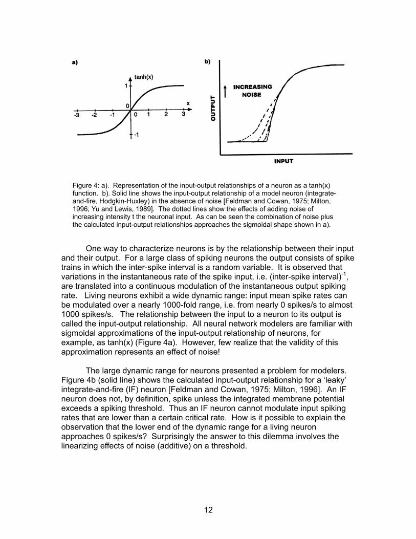
Figure 4: a). Representation of the input-output relationships of a neuron as a tanh(x)

function. b). Solid line shows the input-output relationship of a model neuron (integrate-and-fire, Hodgkin-Huxley) in the absence of noise [Feldman and Cowan, 1975; Milton, 1996; Yu and Lewis, 1989]. The dotted lines show the effects of adding noise of increasing intensity t the neuronal input. As can be seen the combination of noise plus the calculated input-output relationships approaches the sigmoidal shape shown in a).

One way to characterize neurons is by the relationship between their input and their output. For a large class of spiking neurons the output consists of spike trains in which the inter-spike interval is a random variable. It is observed that variations in the instantaneous rate of the spike input, i.e. (inter-spike interval)-1, are translated into a continuous modulation of the instantaneous output spiking rate. Living neurons exhibit a wide dynamic range: input mean spike rates can be modulated over a nearly 1000-fold range, i.e. from nearly 0 spikes/s to almost 1000 spikes/s. The relationship between the input to a neuron to its output is called the input-output relationship. All neural network modelers are familiar with sigmoidal approximations of the input-output relationship of neurons, for example, as tanh(x) (Figure 4a). However, few realize that the validity of this approximation represents an effect of noise!

The large dynamic range for neurons presented a problem for modelers.

Figure 4b (solid line) shows the calculated input-output relationship for a ‘leaky’ integrate-and-fire (IF) neuron [Feldman and Cowan, 1975; Milton, 1996]. An IF neuron does not, by definition, spike unless the integrated membrane potential exceeds a spiking threshold. Thus an IF neuron cannot modulate input spiking rates that are lower than a certain critical rate. How is it possible to explain the observation that the lower end of the dynamic range for a living neuron approaches 0 spikes/s? Surprisingly the answer to this dilemma involves the linearizing effects of noise (additive) on a threshold.

12

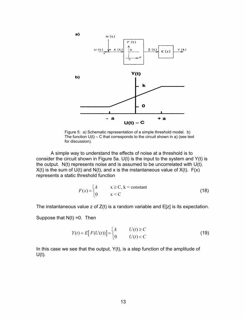
Figure 5: a) Schematic representation of a simple threshold model. b) The function U(t) – C that corresponds to the circuit shown in a) (see text for discussion).

A simple way to understand the effects of noise at a threshold is to

consider the circuit shown in Figure 5a. U(t) is the input to the system and Y(t) is the output. N(t) represents noise and is assumed to be uncorrelated with U(t). X(t) is the sum of U(t) and N(t), and x is the instantaneous value of X(t). F(x) represents a static threshold function

(18) x C, k = constant

( )0 x < Ck

F x≥

=

The instantaneous value z of Z(t) is a random variable and E[z] is its expectation. Suppose that N(t) =0. Then

Y t (19) [ ] ( )( ) ( ( ))

0 ( )k U t

E F U tU t C

≥= = <

C

In this case we see that the output, Y(t), is a step function of the amplitude of U(t).

13

The r

Clearrangeleft). is

and th

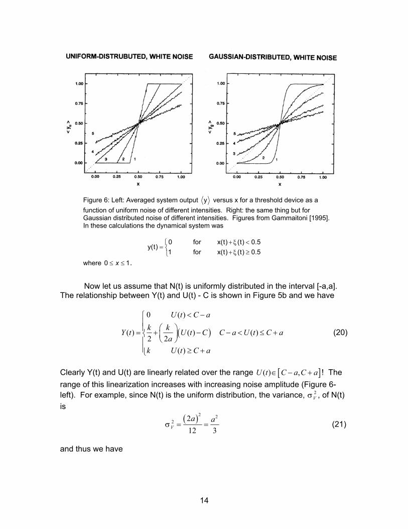
Figure 6: Left: Averaged system output y versus x for a threshold device as a function of uniform noise of different intensities. Right: the same thing but for Gaussian distributed noise of different intensities. Figures from Gammaitoni [1995]. In these calculations the dynamical system was

0 for x(t) (t)

y(t)1 for x(t) (t)

ξξ

+ <= + ≥

0.50.5

where . 0 1x≤ ≤

Now let us assume that N(t) is uniformly distributed in the interval [-a,a].

elationship between Y(t) and U(t) - C is shown in Figure 5b and we have

( )

0 ( )

( ) ( ) ( )2 2

( )

U t C ak k U t C C a U t C a

ak U t C a

< − = + − − < ≤ +

≥ +

Y t (20)

ly Y(t) and U(t) are linearly related over the range U t ! The of this linearization increases with increasing noise amplitude (Figure 6-For example, since N(t) is the uniform distribution, the variance, σ , of N(t)

[ ]( ) ,C a C a∈ − +

2V

( )2 22 2

12 3= =V

a aσ (21)

us we have

14

[ ]3

, 3 ,V

V

a

C a C a C C

σ

σ

=

− + = − + 3 Vσ (22)

Since σ is the rms deviation of the instantaneous amplitude of N(t) from its mean (equal zero in this case) it follows that σ is the rms amplitude of the noise.

V

V

The same result holds if N(t) is a stationary Gaussian random process

with zero mean and standard deviation σ (Figure 6-right). In this case we have

( ) 2

220

1( ) exp2 22

U t Ck k dxσπσ

− = +

∫

xY t (23)

Now if σ is sufficiently large we have

2 2

2 2exp 12 2

1

x xσ σ

≈ − +

≈

…

(24)

and we obtain

(2

1( ) ( )2 2k U t C

πσ= + − )Y t (25)

Figure 4b shows the linearizing effects of additive noise on the input-output relationship of a neuron. In this numerical simulation the input to the neuron is the sum of a DC current plus uniformly distributed white noise. Clearly noise extends the bottom limit of the input-output relationship modulation range to zero yielding the familiar sigmoidal neuronal input-output relationship (Figure 4a). b). Dithering A practical application of the linearizing effects of noise on a threshold arise in the situation that data is collected directly into a computer via an A/D board is now common place [Gammaitoni, 1995]. This process involves two steps: 1) time discretization, and 2) amplitude quantization. Time discretization is the error free step. Two errors enter during amplitude quantization: 1) signal quantization leads to unavoidable distortion, i.e. the presence of spurious signals in a frequency band different from the original one, and 2) loss of signal detail that is small compared to the quantization step (the dynamic range of the digital signal is finite).

15

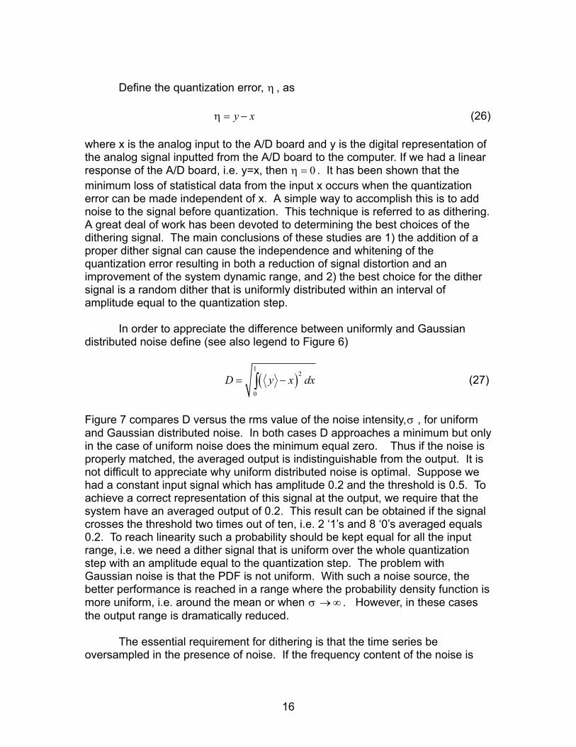
Define the quantization error, η , as

η = (26) y x− where x is the analog input to the A/D board and y is the digital representation of the analog signal inputted from the A/D board to the computer. If we had a linear response of the A/D board, i.e. y=x, then η = . It has been shown that the minimum loss of statistical data from the input x occurs when the quantization error can be made independent of x. A simple way to accomplish this is to add noise to the signal before quantization. This technique is referred to as dithering. A great deal of work has been devoted to determining the best choices of the dithering signal. The main conclusions of these studies are 1) the addition of a proper dither signal can cause the independence and whitening of the quantization error resulting in both a reduction of signal distortion and an improvement of the system dynamic range, and 2) the best choice for the dither signal is a random dither that is uniformly distributed within an interval of amplitude equal to the quantization step.

0

In order to appreciate the difference between uniformly and Gaussian

distributed noise define (see also legend to Figure 6)

( )1

2

0

D y x= −∫ dx (27)

Figure 7 compares D versus the rms value of the noise intensity,σ , for uniform and Gaussian distributed noise. In both cases D approaches a minimum but only in the case of uniform noise does the minimum equal zero. Thus if the noise is properly matched, the averaged output is indistinguishable from the output. It is not difficult to appreciate why uniform distributed noise is optimal. Suppose we had a constant input signal which has amplitude 0.2 and the threshold is 0.5. To achieve a correct representation of this signal at the output, we require that the system have an averaged output of 0.2. This result can be obtained if the signal crosses the threshold two times out of ten, i.e. 2 ‘1’s and 8 ‘0’s averaged equals 0.2. To reach linearity such a probability should be kept equal for all the input range, i.e. we need a dither signal that is uniform over the whole quantization step with an amplitude equal to the quantization step. The problem with Gaussian noise is that the PDF is not uniform. With such a noise source, the better performance is reached in a range where the probability density function is more uniform, i.e. around the mean or when σ → . However, in these cases the output range is dramatically reduced.

∞

The essential requirement for dithering is that the time series be

oversampled in the presence of noise. If the frequency content of the noise is

16

Figure 7: D defined by (28) versus the rms value of the

noise, . The solid line is for Gaussian noise and the dashed line is for uniform noise. Figure from Gammaitoni [1995].

σ much higher than that for the primary signal, then over short intervals the average population of the two quantized levels is a measure of how close the true signal is to the threshold that separates two adjacent bins. Thus it follows that the true signal can be recovered by low-pass filtering (equivalent to averaging) the quantized data. This procedure is illustrated for a noisy pupillometer in Figure 8 [Hunter, et al, 2000]. An analog input signal proportional to pupil diameter (Figure 8a) is discretized in the presence of noise at 25 Hz (Figure 8b). It should be noted that the major frequency components of the open-loop irregular fluctuations in pupil size are 0.3 Hz [Longtin, et al, 1990; Stark, et al, 1958. The quantized signal is then low-passed filtered to yield a time series that closely resembles the original time series (compare Figure 8a to 8c). The main difference is that the low-pass filtering removes the high-frequency components of original signal.

≤

Figure 8: Application of dithering for measuring pupil size in a noisy

pupillometer with low resolution. See text for discussion. Data from Hunter, et al [2000].

c). Stochastic resonance

17

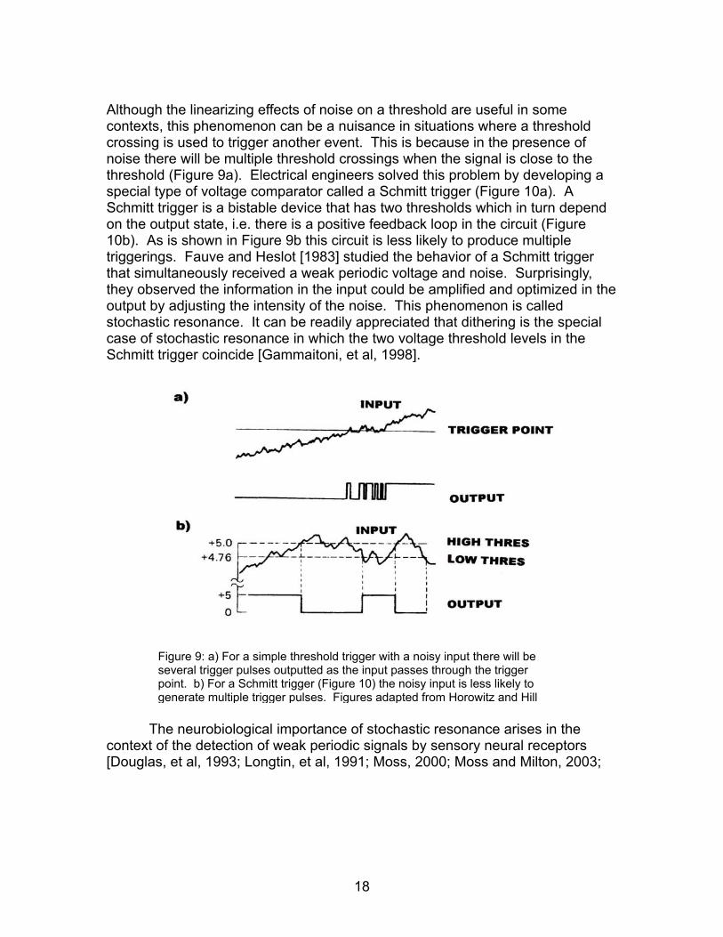
Although the linearizing effects of noise on a threshold are useful in some contexts, this phenomenon can be a nuisance in situations where a threshold crossing is used to trigger another event. This is because in the presence of noise there will be multiple threshold crossings when the signal is close to the threshold (Figure 9a). Electrical engineers solved this problem by developing a special type of voltage comparator called a Schmitt trigger (Figure 10a). A Schmitt trigger is a bistable device that has two thresholds which in turn depend on the output state, i.e. there is a positive feedback loop in the circuit (Figure 10b). As is shown in Figure 9b this circuit is less likely to produce multiple triggerings. Fauve and Heslot [1983] studied the behavior of a Schmitt trigger that simultaneously received a weak periodic voltage and noise. Surprisingly, they observed the information in the input could be amplified and optimized in the output by adjusting the intensity of the noise. This phenomenon is called stochastic resonance. It can be readily appreciated that dithering is the special case of stochastic resonance in which the two voltage threshold levels in the Schmitt trigger coincide [Gammaitoni, et al, 1998].

Tcontext[Dougla

Figure 9: a) For a simple threshold trigger with a noisy input there will be several trigger pulses outputted as the input passes through the trigger point. b) For a Schmitt trigger (Figure 10) the noisy input is less likely to generate multiple trigger pulses. Figures adapted from Horowitz and Hill

he neurobiological importance of stochastic resonance arises in the of the detection of weak periodic signals by sensory neural receptors s, et al, 1993; Longtin, et al, 1991; Moss, 2000; Moss and Milton, 2003;

18

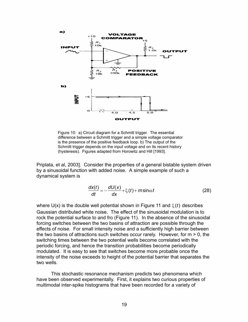
Figure 10: a) Circuit diagram for a Schmitt trigger. The essential

difference between a Schmitt trigger and a simple voltage comparator is the presence of the positive feedback loop. b) The output of the Schmitt trigger depends on the input voltage and on its recent history (hysteresis). Figures adapted from Horowitz and Hill [1993].

Priplata, et al, 2003]. Consider the properties of a general bistable system driven by a sinusoidal function with added noise. A simple example of such a dynamical system is

( ) ( ) ( ) sinξ ω= − + +dx t dU x t m

dt dxt (28)

where U(x) is the double well potential shown in Figure 11 and ξ describes Gaussian distributed white noise. The effect of the sinusoidal modulation is to rock the potential surface to and fro (Figure 11). In the absence of the sinusoidal forcing switches between the two basins of attraction are possible through the effects of noise. For small intensity noise and a sufficiently high barrier between the two basins of attractions such switches occur rarely. However, for m > 0, the switching times between the two potential wells become correlated with the periodic forcing, and hence the transition probabilities become periodically modulated. It is easy to see that switches become more probable once the intensity of the noise exceeds to height of the potential barrier that separates the two wells.

( )t

This stochastic resonance mechanism predicts two phenomena which have been observed experimentally. First, it explains two curious properties of multimodal inter-spike histograms that have been recorded for a variety of

19

neurons including retinal ganglion neurons in the cat [Sanderson, et al, 1973] and in auditory fibers of monkeys [Rose, et al, 1967] (Figure 12a): 1) the modes occur at an integer multiple of a fundamental period; and 2) the mode amplitude decreases approximately exponentially.

Figure 11: A suitable dose of noise (i.e. when the period of the driving approximately equals twice the noise-induced escape time) will make the “sad” face” happy by allowing synchronized hopping to the attractor with the lower energy. Strictly speaking, this holds true only for the statistical average. Figure taken from Gammaitoni, et al [1998]. Why? It’s really a fun figure!

Second, the signal to noise ratio (SNR) for a stochastically resonant dynamical system exhibits a non-monotone dependence on noise intensity. As the intensity of the noise increases the output of the sensory neuron increases (Figure 12b). This is because switches between the basins of attraction are possible only if noise is present. The SNR reaches a maximum at roughly the point where the noise intensity is on average sufficient to cause a transition at the point in time when the potential barrier between the basins of attraction is most shallow. Thereafter, further increases in noise intensity deteriorate the SNR (as is always the case in dynamical systems that do not exhibit stochastic resonance).

20

Figure 12: a) Interspike histogram measured from a single auditory nerve fiber of a squirrel monkey with sinusoidal 80-dB sound-pressure-level stimulus of period T0 = 1.66 ms applied at the ear (Rose, et al, 1967). b) Signal-to-noise ratio of a hydro-dynamically sensitive hair mechano-receptor in the tail of a crayfish in the presence of periodic water motion to which noise has been added of increasing intensity (Douglas, et al, 1993).

d). Spike time reliability Typically the input of a neuron does not contain a strong periodic component but is a rather complex aperiodic signal. Such inputs can be represented as having both a DC, or constant, component and an AC, or time-varying, component. The

21

neuron’s firing rate ( f ) in response to the DC component places constraints on the types of signals that may be encoded reliably in the presence of noise. This effect is currently studied under the heading “spike timing reliability”.

DC

Spike timing reliability refers to the precision of spike timing when a

spiking neuron is repeatedly given the same time-varying input. In 1995 Mainen and Sejnowski made a surprising observation concerning the spike-timing reliability of neocortical neurons. Namely, precisely timed spike trains are produced by neurons in response to aperiodic input signals in which current fluctuations resemble synaptic activity, but not when they receive a constant-current stimulus. Again the interpretation of this phenomenon involves considerations of the effects of noise on the input-output relationship of a neuron.

coca

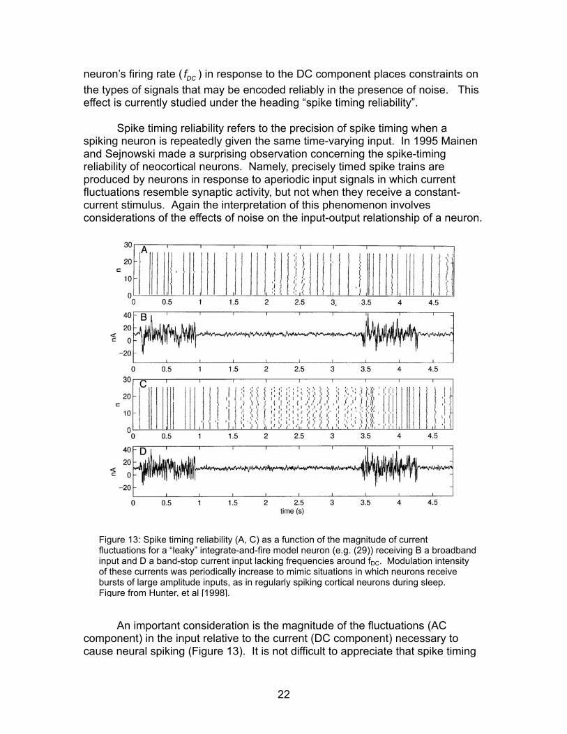
Figure 13: Spike timing reliability (A, C) as a function of the magnitude of current fluctuations for a “leaky” integrate-and-fire model neuron (e.g. (29)) receiving B a broadbandinput and D a band-stop current input lacking frequencies around fDC. Modulation intensof these currents was periodically increase to mimic situations in which neurons receive bursts of large amplitude inputs, as in regularly spiking cortical neurons during sleep. Fi

ity

gure from Hunter, et al [1998].

An important consideration is the magnitude of the fluctuations (AC mponent) in the input relative to the current (DC component) necessary to use neural spiking (Figure 13). It is not difficult to appreciate that spike timing

22

will be reliable when the relative magnitude of the input fluctuations is high. In the presence of noise, the width of inter-spike interval distributions is inversely proportional to the slope of the membrane potential at threshold [Goldberg, et al, 1984; Stein, 1967]. A current with a large-amplitude fluctuating component will cause threshold crossings with a steeper slope than will a constant current and thus generate more reliably timed spikes in the presence of noise. An analogous slope condition exists for the synchronization of a network of neurons to a coherent input [Gerstner, et al, 1996] and also explains the increased variability of the period of pupil cycling when the threshold is set close to the maximum pupil area [Longtin, et al, 1990; Milton and Longtin, 1990].

i

Figure 14: ‘Leaky’ integrate-and-fire model neuron (e.g. (29)) with constant and periodic inputs. A: membrane current in response to a DC input current, B: membrane potential with current modulated at , and C: trajectory modulated by . The dashed horizontal lines indicate the threshold for spiking, D-F the distribution of spike times obtained for the currents in G-I in the presence of noise. For each input, initial conditiowere chosen to trigger a spike at time 0 in the absence of noise resulting in a peaked spike time distribution around 0 when noise is added. Note that the first peak in the spike distribution is sharper in response to the sinusoidal currents (E and F) than in response to a DC input (D) because the slope of the membrane potential at threshold crossing is steepsince the initial conditions were chosen so that the first spike in the deterministic case wouldoccur at the same phase of the sinusoids. At the second threshold crossing, the slopmembrane potential in C is steeper than in A or B. This results in a narrower spike time distribution in the presence of noise. Figure from Hunter, et al [1998].

DCf / f 0.65= DCf / f 1=

ns

er

e of the

However, when the fluctuating component of the input is relatively small it

s also possible for spike-timing reliability to arise from a resonance phenomenon

23

(Figure 14) [Hunter, et al, 1998; Hunter and Milton, 2002, 2003]. Suppose at time 0 a spike occurs on the rising phase of an input signal and the membrane potential is reset to rest. If the time-varying component of the input is small compared with the DC component, then the next spike will not occur until some time approximately equal to T , the inverse of f . If the time-varying component of the input signal is increasing around time T , the spike time distribution will be narrower that if the time-varying component is decreasing at this time because of the above slope considerations.

DC DC

DC

It follows that spike-timing reliability will be highest when the aperiodic

input contains frequencies of the order of [Bryant and Segundo, 1976; Collins, et al, 1995; Hunter, et al, 1998; Knight, 1972; Jensen, 1998]. Figure 15 shows that this is true. This figure shows spike timing reliability8 of an Aplysia motoneuron to three different aperiodic signals: 1) broadband, low-pass filtered noise (Figure 15a); 2) broadband, low-pass filtered noise in which the frequencies around and including f were removed (Figure 15b); and 3) a broadband, low-pass filtered noise in which a frequency band below f was removed (Figure 15c). Spike timing reliability is highest provided that the input contains frequencies around f .

DCf

DC

DC

DC

Figure 15: Spike time reliability (right) for an Aplysia motoneuron to different aperiodic inputs (left). See text for discussion. Figure from Hunter and Milton [2002].

8 A convenient measure of spike time reliability is the reliability statistic, , calculated as the time-series variance normalized so that it ranges from zero to one [Hunter, et al, 1998; Hunter and Milton, 2003].

ℜ

24

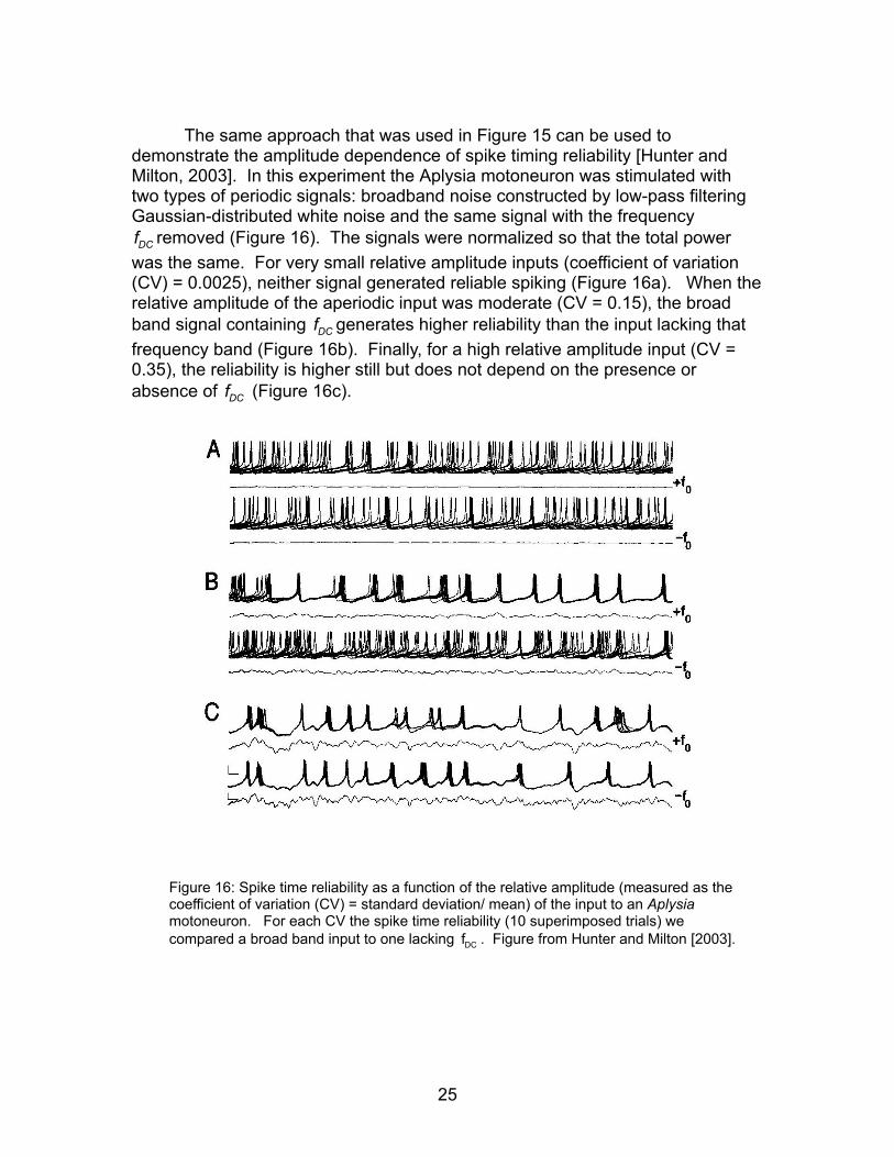
The same approach that was used in Figure 15 can be used to

demonstrate the amplitude dependence of spike timing reliability [Hunter and Milton, 2003]. In this experiment the Aplysia motoneuron was stimulated with two types of periodic signals: broadband noise constructed by low-pass filtering Gaussian-distributed white noise and the same signal with the frequency

removed (Figure 16). The signals were normalized so that the total power was the same. For very small relative amplitude inputs (coefficient of variation (CV) = 0.0025), neither signal generated reliable spiking (Figure 16a). When the relative amplitude of the aperiodic input was moderate (CV = 0.15), the broad band signal containing generates higher reliability than the input lacking that frequency band (Figure 16b). Finally, for a high relative amplitude input (CV = 0.35), the reliability is higher still but does not depend on the presence or absence of f (Figure 16c).

DCf

DCf

DC

Figure 16: Spike time reliability as a function of the relative amplitude (measured as the coefficient of variation (CV) = standard deviation/ mean) of the input to an Aplysia motoneuron. For each CV the spike time reliability (10 superimposed trials) we compared a broad band input to one lacking . Figure from Hunter and Milton [2003]. DCf

25

The observations in Figure 16 can be reproduced by studying the response of a leaky integrate-and-fire neuron model to inputs, I(t), constructed from modulated Poisson processes [Hunter and Milton, 2003]

= − + + σξdV V(t) RI(t) (t)dt

RC (29)

where V(t) is the membrane potential, R is the membrane resistance, C is the membrane capacitance, ξ is Gaussian distributed noise with unit standard deviation scaled by σ . In integrating (29) it is assumed that when he neuron produces a spike and the membrane potential is reset to its resting potential. Modulated Poisson processes arise in the description of neural spike trains in which the probability of neural firing varies with time [Burkitt and Clark, 2000; Perkel and Bullock, 1968; Tuckwell, 1989]. The advantage of this signal is that the power spectra and SNR at the modulation frequency are known in closed form [Bartlett,1963; Bayly, 1968; Knox, 1970]. The modulation rate is given by

(t)≥ θV t

ra (30) (0( ) 1 sin(2 )mte t m f tλ= + )π

where is the carrier rate, is the modulation amplitude, and f is the modulation frequency. It is assumed that the carrier rate is sufficiently low that the probability of spiking twice in a single time interval is small. In order to introduce a periodically modulated spike train input into (29), we took

0λ 0 1m≤ ≤ m

I (31) ( )= + δ − − λ

∑ k 0

k(t) DC i t t

where is the Dirac-delta function, are the spike times from the Poisson process with modulated given by (30), and I is the event amplitude. It should be noted that changes in the carrier rate affect the average spiking rate of the neuron and hence the location of the resonance peak. The offset λ removes this confounding factor.

δ(t) kt

0

A realization of a neural spike train of a neural spike train generated by a

periodically modulated Poisson process is show in Figure 17A, and its power spectral density in Figure 17B. The power spectral density, S(f), is

(2 2 20 0 0

1( ) ( )4 mf m f fλ λ δ λ δ= + + − )S f (32)

where is the Dirac delta function. The broadband, background power is the same at all frequencies and equals . The power at the modulation frequency is

and hence the SNR is proportional to λ . The spike time reliability for

δ

/ 40λ

20mλ 2 2

0 m

26

the IF neurons receiving the modulated Poisson input plus additive noise is shown in Figure 17C. As can be seen there is a monotonic relationship between Rand . An analogous effect is seen if the modulation depth is held constant and the modulation frequency is varied. In this case there is a resonance peak seen only for moderate amplitudes (Figure 17D).

20mλ

Figure 17: Modulated Poisson input current generates three relative amplitude regimes for spike-timing reliability. See text for discussion. Figure from Hunter and Milton [2003]

The important point about spike timing reliability is that it emphasizes that the encoding properties of a neuron depends on both the intrinsic properties of the neuron and the nature of the input. Thus the same neuron can be either a rate or a spike time encoder. Moreover there exists a range of input modulation amplitudes for which small modifications in either the frequency content of the input or the firing rate of the neuron can dramatically alter spike timing reliability. This leads to a rate-control mechanism for neural synchrony [Hunter and Milton, 2002, 2003]. III. Parametric noise In the nervous system the effects of noise typically are state-dependent. For example, membrane noise reflects fluctuations in conductance and hence its effect on current (proportional to the product of conductance and the driving potential) is state-dependent [Chance, et al, 2002; Verveen and De Felice, 1974]. State-dependent noise underlies the spontaneous fluctuations in pupil size [Stark, et al, 1958] and plays important roles in motor [Harris and Wolpert, 1998; Jirsa, et al, 2000] and balance [Cabrera and Milton, 2002; Cabrera, et al, 2004] control. Indeed it is quite difficult to think of an effect of noise on the nervous system that is not state dependent!

27

One way to account for these state-dependent effects of noise is to

assume that the noise enters through parameters. It must be remembered that in modeling those variables that change much more slowly than others are typically held constant (hence are parameters). However, experimentally it is typically found that those variables designated as parameters in a model themselves vary (see, for example, Milton, et al, 1989) thus blurring the traditional distinction between variable and parameter. It is obvious that parametric noise will have much greater effects on a dynamical system than additive noise. This is because the parameters determine the shape of the “potential surface” on which the dynamics evolve. If parameters change as an effect of the noise, then this means that this potential surface is itself continually changing. Here lies the problem.

Many of the same effects observed for dynamical systems subjected to

additive noise have their analogues in dynamical systems subjected to parametric noise [Milton, et al, 2004]. For example, although we have discussed stochastic resonance in the context of additive noise, the same phenomena occurs in dynamical systems subjected to the effects of parametric noise (for a review see [Gammaitoni, et al 1998]). An exception arises in the case that a parameter is stochastically forced back and forth across a stability boundary [Cabrera and Milton, 2002; Heagy, et al, 1994; Platt, et al, 1993]. In this case phenomena arise which do not have an analog in dynamical systems with additive noise. These phenomena are discussed here under the heading “on-off intermittency”.

To illustrate the added complexities that arise consider parametric Langevin equation

( ) ( ) ( ) ( )= +dx t t x t t

dtη ξ (33)

where x(t) is a dynamic variable, η is parametric white noise with mean ( )t η and intensity D , and ξ is additive white noise with mean zero and intensity . It has been shown [Deutsch, 1994; Venkataramani, et al, 1996; Nakao, 1998; Sato, et al, 2000a; Takayasu, et al, 1997] that the stationary probability density p(x) is

η ( )t Dξ

( )1

2 2( ) Dp x D D x η

η

ξ η

−≈ + 2 (34)

and that the tails for large x exhibit power laws of the form 1( )p x x β− −

≈ (35)

28

where / Dηβ η= − . There are two important observations: 1) the power law exponent depends only on the statistical properties of the parametric noise, in particular its mean and intensity; and 2) the power laws can be observed for a completely linear dynamical system.

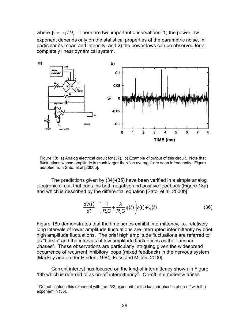
Figure 18: a) Analog electrical circuit for (37). b) Example of output of this circuit. Note that fluctuations whose amplitude is much larger than “on average” are seen infrequently. Figure adapted from Sato, et al [2000b].

The predictions given by (34)-(35) have been verified in a simple analog electronic circuit that contains both negative and positive feedback (Figure 18a) and which is described by the differential equation [Sato, et al, 2000b]

( ) 1 ( ) ( ) ( )η

= + + f v

dv t k t v t tdt R C R C

ξ

(36)

Figure 18b demonstrates that the time series exhibit intermittency, i.e. relatively long intervals of lower amplitude fluctuations are interrupted intermittently by brief high amplitude fluctuations. The brief high amplitude fluctuations are referred to as “bursts” and the intervals of low amplitude fluctuations as the “laminar phases”. These observations are particularly intriguing given the widespread occurrence of recurrent inhibitory loops (mixed feedback) in the nervous system [Mackey and an der Heiden, 1984; Foss and Milton, 2000].

Current interest has focused on the kind of intermittency shown in Figure 18b which is referred to as on-off intermittency9. On-off intermittency arises

29

9 Do not confuse this exponent with the -3/2 exponent for the laminar phases of on-off with the exponent in (35).

because of the stochastic or chaotic forcing of a parameter back and forth across a stability boundary. This type of intermittent behavior is distinct from the intermittency observed in deterministic dynamical systems such as Pomeau-Manneville type-I, -II, and –III intermittency and crisis-induced intermittency. These types of intermittency occur for fixed values of the parameters while in on-off intermittency the bifurcation parameter is itself a dynamical variable. The implication of the detection of on-off intermittency experimentally is that it implies that the underlying dynamical system must be tuned in parameter space to be close to a stability boundary. How close? This depends on the intensity of the parametric noise. A particularly insightful discussion into the effects of parametric noise on discrete time dynamical systems was developed by Heagy, Platt and Hammel [1994]. Here we briefly outline their presentation. The interested student who wishes more details should consult the original source. We then discuss on-off intermittency in an experimental system, namely, stick balancing at the fingertip, and then briefly discuss the rather surprising implications for the neural control of movement. a). On-off intermittency in the quadratic map Consider a quadratic map with parametric noise, i.e. (37) (1 ( ) 1+ =t t tx xλ ξ )− tx

t

tx

where λ ξ (38) ( ) ( )t ay ξ= where a is a constant and is a random variable drawn from a uniform density on the interval [0,1]. This map produces intermittency for an appropriate value of a (Figure 19). Numerical experiments indicate that the longer the laminar phases, the smaller the magnitude of the fluctuations. This observation was interpreted as implying that the dynamics are almost completely determined by the linear part of the map. The nonlinear terms serve only to bound or re-inject the dynamics back toward small values of x. In other words the nonlinearities are essential for sustaining the intermittent behavior, but not for initiating the bursts.

( )ty ξ

If we consider only a linear map, (39) 1 ( ) ,+ =t tx λ ξ

30

Figure 19: On-off intermittency in the quadratic map for a=2.8.

then we know that its long time behavior is given by

(40) 1

00

n

nj

x λ−

=

=∏ j x

j

where is the value of x at t = 0. Consequently the long term behavior is determined by the asymptotic behavior of the random product

0x

Ψ = (41) 1

0

n

nj

λ−

=∏

Taking logarithms and making use of the law of large numbers10 we obtain

1

0ln ln

n

n jj

nλ−

=

Ψ = ≈∑ln (42) λ

Since we have assumed that the density of the distribution for the parametric noise is uniform we can readily calculated the statistical average as

0 0

ln ( )ln ln ln 1a a

up d d aλ λ λ λ λ λ= = =∫ ∫ −

(43)

Thus we see that the asymptotic solution of (39) is

10 The law of large numbers states that the arithmetic average of a very large sum of independent observations of a random variable x(s) is equal to the mean of x(s). It is a corollary of the Central Limit Theorem (Chung, 1975).

31

ln0

nn

nax e x xe

λ ≈ =

0 (44)

It follows that the condition for intermittent behavior is ln 0λ = . When ln 0λ > , the fixed-point is, on average, exponential unstable. This

instability is the source of the intermittent bursts. However, we must remember that this is just a local result. Thus this instability does not preclude the occurrence of long orbit segments in the neighborhood of x = 0, i.e. the laminar phases. The critical value of a for the onset of intermittency is

0x =

a (45) 2.71828≈

b). 32−power laws

Taking the logarithm of (39) we obtain (46) n 1 n n

ˆy + = λ + y

0

where and . A laminar phase of length n is defined by y ln(x)= ˆ ln( )λ = λ [ ] (47) 1 0 2 0 n 0 n 1 0y y ,y y , ,y y ,y y+≤ ≤ ≤ >… Since (46) is translationally invariant we can define without loss of generality the threshold as . The probability that a laminar phase has exactly length n is given by the conditional probability

0y =

n

n j n 1j 1

Pr ob y 0 y 0 y 0+=

≤ > ≤

∩ ∩ 1 Λ = (48)

The laminar phase of length n corresponds to an event for which the product in (41) remains less than or equal to zero for exactly n iterations and becomes greater than one on the n+1st iteration. Using the decomposition rule

Pr ob(A B)

ob(A | B)Pr ob(B)

= ∩Pr

we can rewrite (48) as

32

( )

n

j j 1j 1

n1

Pr ob y 0 y 0

Pr ob y 0

+=

≤ >

Λ =≤

∩ ∩ (49)

If we define

g P n

n jj 1

r ob s 0=

≡ ≤

∩

Then we can rewrite (49) as

n n 1n

1

g gProb(y 0)

+−Λ =

≤ (50)

Since the computation of is an example of a recurring event, we can use a generating function11, G(t), to estimate the probability g

ng

n

G( (51) nn

n 0t) g t

∞

=

= ∑ It is shown in Feller [1971] that

[ ]n

nn 1

tG(t) Pr ob(y 0)n

∞

=

= ∑ln (52) ≤

Since λ is chosen from a uniform distribution we know that the probability density is symmetric about the origin (zero in this case). Thus we have

ˆ

n1ob(y 0)2

≤ =Pr (53)

11 Generating functions frequently arise in the description of recurrent events, i.e. stochastic processes that are generated by a repetitive series of experimental trials such as coin flipping [Bailey, 1963]. If we have a sequence of real numbers a , , then we can write 0 1 2a ,a ,

2 j0 1 2 j

j 0A(x) a a x a x a x

∞

=

= + + + = ∑where x is a dummy variable. If this series converges in some interval , then the

function A(x) is called the generating function of the sequence { . The generating function can

be regarded as a transformation carrying the sequence { into the function A(x).

0 0x ,x−

}jx

}jx

33

and (52) becomes12

[ ]n

n 1

1 t 1G(t) ln2 n 1 t

∞

=

= = − ∑ln

or

1G(t)1 t

=−

(54)

The coefficients in (52) can be evaluated from

n

n n 2nt 0

1 G(t) (2n)!n! t 2 (n!)

=

∂= =

∂ 2g

The numerator of (50) becomes

3 / 2nn n 1

g 1g g n2(n 1) 2

−+− =

+ π∼ (55)

where the last relation follows from Stirling’s approximation13. Thus we see that at onset the laminar phases, Λ , decay as a power law with exponent -3/2. This result has been extended to include all probability densities for the distribution

that have zero mean and finite variance [Heagy, et al, 1994].

n

λ̂ c). Stick balancing at the fingertip

The study of stick balancing at the fingertip is important for understanding the neural control of balance [Cabrera and Milton, 2002; Foo, et al, 2000; Mehta and Schaal, 2002; Treffner and Kelso, 1999] and the development of expertise [Cabrera and Milton, 2004b; Cabrera, et al, 2004; Mah and Mussa-Ivaldi, 2003a,b; Milton, et al, 2004]. This task is particularly relevant to our discussion of the effects of parametric noise since it is well known that when the pivot point of an inverted pendulum moves, either periodically [Bogdanoff, 1962; Bogdanoff and Citron, 1964] or noisily [Landa, et al, 1998], the perturbations enter the equations through their effects on a parameter14. There are also a number of

12 This result is obtained by differentiating the sum on the right hand side of (53), then summing the resultant geometric series, and integrating. 13 Stirling’s approximation is n nn! 2 ne n−π∼ . 14 For example, if the pivot point of an inverted pendulum is made to vibrate up and down then the effect of gravity is lessened by an amount , i.e. 2g d h / dt− 2

34

advantages offered by the study of stick balancing at the fingertip as an experimental paradigm: 1) the movements can be measured with high precision using 3-D motion analysis techniques [Cabrera and Milton, 2002, 2004b]; 2) mathematical models for the control of inverted pendulums with time-delayed feedback have been extensively studied [Landray, et al, 2004; Stépán, 1989; Stépán and Kollár, 2000]; 3) virtual stick balancing tasks that involve a human interacting with a computer have been developed which enable critical parameters to be precisely manipulated [Bormann, et al, 2004; Cabrera, et al, 2004; Mah and Mussa-Ivaldi, 2003b; Mehta and Schaal, 2002]; 4) skill level can be objectively determined by, for example, measuring the fraction of sticks that can be balanced longer than a certain time [Cabrera and Milton, 2004a,b; Cabrera, et al, 2004]; and 5) skill level can be significantly increased with just a few days of intensive practice [Cabrera and Milton, 2004b; Cabrera and Milton, 2003, 2004]. The importance of the time delay for stick balancing is demonstrated by the observation that longer sticks are easier to balance than shorter ones: once the stick becomes sufficiently long its rate of movement becomes slow relative to the time required by the nervous system to make corrective movements. Indeed mathematical models for the stabilization of an inverted pendulum with time delayed feedback suggest that in order to balance a stick of length, , the time delays must be less than a critical value proportional to [Stépán, 1989; Stépán and Kollár, 2000].

The fluctuations in the controlled variable, θ, exhibit on-off intermittency [Cabrera and Milton, 2002]. This observation is supported by the presence of a –1/2-power law [Venkataramani, et al, 1996] in the power spectrum of the fluctuations in θ (Fig. 19a) and a –3/2 power law for the laminar phases (Fig. 19b). The observation of on-off intermittency suggests that the neural control mechanism for stick balancing is tuned at the edge of stability: this phenomenon arises because of the stochastic or chaotic forcing of an important parameter across a stability boundary [Cabrera and Milton, 2002; Heagy, et al, 1994; Platt, et al, 1993]; the proximity to the stability boundary depending on the intensity of the noise.

The observations in Fig. 19 can be reproduced by the equation of motion

for an inverted pendulum stabilized by time-delayed feedback with a noisy gain [Cabrera and Milton, 2002], i.e.

2 2

2 2d g d h sin 0dt dt

θ+ − θ =

2 2h / dtwhere d denotes the downward acceleration of the pivot and g the acceleration due to gravity [Acheson, 1997]. This is why we feel we feel less heavy than usual if we are in an elevator which is accelerating downwards!

35

2

02d (t) d (t)e qsin (r (t)) (t

dt dt= − + − + −

θ θθ ξ θ )τ (56)

Figure 20: a) Power spectrum, S(f), of the fluctuations in the vertical displacement angle for stick balancing at the fingertip. The frequency is f. The solid lines have slope, respectively, -0.5 and -2.5. The small peak at 1-2 Hz is norelated to the phenomena we discuss here [Cabrera and Milton, 2002]. b) Log-log plot showing the normalized probability of having laminar p s

t

ha es of length t,δ P( t)δ . Note that in stick balancing the latency is 100-200 ms. Figure from Cabrera, et al [2004].

where e,q,r0 are constants and ξ(t) is Gaussian-distributed, white noise. Although a feedback term that does not contain a velocity term might initially concern investigators who study motor control, it should be noted that a delayed controller shares features with derivative feedback in modifying the behavior of the system15. In contrast to an inverted pendulum, an inverted pendulum with delayed feedback has a stable upright position [Cabrera and Milton, 2002; Landray, et al, 2004; Stépán, 1989; Stépán and Kollár, 2000]. The essential condition for (56) to reproduce the observations in Fig. 19 is that the parameters r0 and q be chosen sufficiently close to the appropriate stability boundary [Cabrera and Milton, 2002]. The observation that on-off intermittency arises in stick balancing at the fingertip has several implications concerning how the nervous system might 15 From the definition of a derivative we have d (t)(t ) (t)

dt− ≈ −

θθ τθ τ .

36

control this task. First, on-off intermittency provides a mechanism that enables corrective movements to be made on time intervals shorter than the neural delay (> 98% of the δ in Figure 20 are shorter than the delay - see figure legend and [Cabrera and Milton, 2002]). Second, on-off intermittency provides a mechanism of non-predictive control for stick balancing, i.e. the fluctuations in θ resemble a random walk for which the mean value of θ is approximately zero, i.e. the upright position has been statistically stabilized [Cabrera and Milton, 2002, 2003, 2004a,b]. The fact that the movements of the fingertip during stick balancing can be described as a Lévy flight with α ≈ emphasizes the non-predictive aspects of the control strategy [Cabrera and Milton, 2004b]. Finally, the existence of a non-predictive control mechanism for stick balancing reduces the demands on intentionally directed control mechanisms and thus “frees up” the conscious and attentional mechanisms of the brain for other tasks [Cabrera and Milton, 2004a,b; Cabrera, et al, 2004; Milton, et al, 2004].

t

0.9

IV. Concluding Remarks:

It must be remembered that comparing the prediction of a model to experimental observation is an essential component of the scientific method. Such comparisons are not particularly useful unless the effects of noise on the predictions of the model are carefully investigated. Moreover, the fact that measurements of the statistical properties of the fluctuations can provide important non-invasive insights into the structure of the underlying dynamical system is likely to have increasing important as regulatory burden placed on human subject research increase, particularly in the study of normal physiology. Acknowledgements The author thanks John D. Hunter for proof reading this manuscript and helpful comments. Research was supported by grants from the National Institutes of Mental Health and the Brain Research Foundation. References: Acheson D (1997). From Calculus to Chaos: An Introduction to Dynamics. Oxford

University Press, New York. Areili A, Sterkin A, Grinald A and Aertson A (1996). Dynamics of ongoing activity: explanation for

the large variability in evoked potential responses. Science 273: 1868-1871. Bailey NTJ (1964). The Elements of Stochastic Processes. Wiley Classics Library Edition

(1990). John Wiley & Sons, Toronto. Bartlett MS (1963). The spectral analysis of point processes. J. Roy. Stat. Soc. B 25: 264-280. Bayly EJ (1968). Spectral analysis of pulse frequency modulation in the nervous system. IEEE

Trans. Biomed. Eng. 15: 257-265. Bendat JS and Piersol AG (1986). Random Data: Analysis and Measurement Procedures, 2nd

Edition. John Wiley & Sons, Toronto. Bogdanoff JL (1962). Influence on the behavior of a linear dynamical system of some imposed

rapid motions of small amplitude. J. Acoust. Soc. Amer. 34: 1055-1062. Bogdanoff L and Citron SJ (1964). Experiments with an inverted pendulum subject to rapid

parametric excitation. J. Aocust. Soc. Amer. 38: 447-452.

37

Bormann R, Cabrera JL, Milton JG and Eurich CW (2004). Visuomotor tracking on a computer screen: An experimental paradigm to study the dynamics of motor control, Neurocomputing (in press).

Borsellino A, De Marco A, Allazetta A, Rinsei S and Bartolini B (1972). Reversal time distribution of visual ambiguous stimuli. Kybernetik 10:139-144.

Bracewell RN (1986). The Fourier Transform and Its Applications. McGraw-Hill, Toronto. Brigham EO (1988). The Fast Fourier Transform and its Applications. Prentice Hall, Englewood

Cliffs, New Jersey. Brockman B and Geisel T (2000). Ecology of gaze shifts. Neurocomputing 32-33: 643-650. Brockman B and Geisel T (2003). Lévy flights in inhomogeneous media. Phys. Rev. Lett. 90:

170601. Bryant HL and Segundo JP (1976). Spike initiation by transmembrane current: a white-noise

analysis. J. Physiol. 260: 279-314. Buldyrev SV, Havlin S, Kazakov A Ya, da Lu MGE, Raposo EP, Stanley HE and Viswanathan GM

(2001). Average time spent by Lévy flights and walks on an interval with absorbing boundaries. Phys. Rev. E 64: 041108.

Burkitt AN and Clark GM (2000). Calculation of interspike intevrals for integrate and fire neurons with Poisson distribution of synaptic inputs. Neural Computat. 12: 1789-1820.

Cabrera JL, Bormann R, Eurich C, Ohira T and Milton J (2004). State-dependent noise and human balance control. Fluctuations Noise Lett. 4: L107-L118.

Cabrera JL and Milton JG (2002). On-off intermittency in a human balancing task. Phys. Rev. Lett. 89: 58702-1-4.

Cabrera JL and Milton JG (2003). Delays, scaling and the acquisition of motor skill. In Bezrukov, S, ed. Unsolved Problems of Noise and Fluctuations: UpoN 2002: Third International Conference on Unsolved Problems of Noise and Fluctuations in Physics, Biology and High Technology (AIP Proceedings 665, American Institute of Physics, Melville, NY), pp. 250-256.

Cabrera JL and Milton JG (2004a). Stick balancing: On-off intermittency and survival times. Nonlinear Studies 11(3): in press.

Cabrera JL and Milton JG (2004b). Human stick balancing: Tuning Lévy flights to improve balance control. CHAOS (accepted).

Calvin WH and Stevens CF (1968). Synaptic noise and other sources of randomness is motoneuron interspike intervals. J. Neurophysiol. 31: 574-587.

Chance FS, L. F. Abbott LF and A. D. Reyes AD (2002). Gain modulation from background synaptic input. Neuron 35: 773-782.

Chung K (1975). Elementary Probability with Stochastic Processes. Spinger-Verlag, New York. Collins JJ, Chow CC and Imhoff TT (1995). Stochastic resonance without tuning. Nature

(London) 376: 236-238. Davenport WB and Root WL (1987). An Introduction to the Theory of Random Signals and

Noise. IEEE Press, New York. Deutsch JM (1994). Probability distributions for one component equations with multiplicative

noise. Physica A 246 430-444. Douglas JK, Wilkens L, Pantazelou E and Moss F (1993). Noise enhancement of information

transfer in crayfish mechanoreceptors by stochastic resonance, Nature (London) 365: 337-340.

Eurich CW and Milton JG (1996). Noise-induced transitions in human postural sway. Phys. Rev. E. 54: 6681-6684.

Evans M, Hastings N ad Peacock B (1993). Statistical Distributions, 2nd Edition. John Wiley & Sons, Toronto.

Fatt P and Katz B (1950). Some observations on biological noise. Nature (London) 166: 597-598. Fauve S and Heslot F (1983). Stochastic resonance in a bistable system. Phys. Lett. A 97: 5-7. Feldman JL and Cowan JD (1975). Large-scale activity in neural nets. I. Theory with application

to motoneuron pool responses. Biol. Cybern. 17: 29-38. Feller W (1971). An Introduction to Probability Theory and Its Applications, Volume II, Second

Edition. John Wiley & Sons, Toronto. Foo P, Kelso JAS and de Guzman GC (2000). Functional stabilization of fixed points: Human

38

pole balancing using time to balance information. J. Exp. Psychol: Human Percept. Perform. 26: 1281-1297.

Foss J and Milton J (2000). Multistability in recurrent neural loops arising from delay. J. Neurophysiol. 84: 975-985.

Foss J, Moss F and Milton J (1997). Noise, multistability and delayed recurrent loops. Phys Rev. E 76: 708-711.

Gammaitoni L (1995). Stochastic resonance and the dithering effect in threshold physical systems. Phys. Rev. E 52: 4691-4698.

Gammaitoni L, Hänggi P, Jung P and Marchesoni F (1998). Stochastic resonance. Rev. Modern Phys. 70: 223-287.

Gardiner CW (1990). Handbook of Stochastic Methods. Springer-Verlag, New York. Gerstner W, van Hemmen JL and Cowan JD (1996). What matters in neuronal locking? Neural

Comput. 8: 1653-1676. Goldberg J, Smith CE and Fernández C (1984). Relation between discharge regularity and

responses to externally applied galvanic currents in vestibular nerve afferents of the squirrel monkey. J. Neurophysiol. 51: 236-1256.

Harris CM and Wolpert DM (1998). Signal-dependent noise determines motor planning. Nature (London) 394: 780-784.

Heagy JF, Platt N and Hammel SM (1994). Characterization of on-off intermittency. Phys. Rev. E 49: 1140-1150.

Horowitz P and Hill W (1993). The Art of Electronics, Second Edition. Cambridge University Press, New York.

Horsthemke W and Lefever R (1984). Noise-induced transitions: Theory and Applications in Physics, Chemistry and Biology. Springer-Verlag, New York.

Hunter JD, Milton JG, Ludtke H, Wilhelm B, and Wilhelm W (2000). Spontaneous fluctuations in pupil size are not triggered by lens accommodation. Vision Res. 40: 567-573.

Hunter JD, Milton JG, Thomas P, and Cowen JD. (1998). A resonance effect for neural spike timing reliability. J. Neurophys. 80: 1427-1438.

Hunter JD and Milton J (2002). Using inhibitory interneurons to control neural synchrony. In: Epilepsy as a Dynamic Disease (J. Milton and P. Jung, eds.) Springer-Verlag: New York, pp. 115-130.

Hunter JD and Milton JG (2003). Amplitude and frequency dependence of spike timing: Implications for dynamic regulation. J. Neurophysiology 90: 387-394.

Jenkins GM and Watts DG (1968). Spectral Analysis and its Applications. Emerson-Adams Press. Boca Raton, Florida.

Jensen RV (1998). Synchronization of randomly driven nonlinear oscillators. Phys. Rev. E 58: 6907-6910.

Jirsa VK, Fink P, Foo P and Kelso JAS (2000). Parametric stabilization of biological coordination: a theoretical model. J.Biol. Phys. 26: 85-112.

Kloeden PE and Platen E (1992). Numerical Solution of Stochastic Differential Equations. Springer-Verlag, New York. Knight BK (1972). Dynamics of encoding in a population of neurons. J. Gen. Physiol. 59: 734-

766. Knox CK (1970). Signal transmission in random spike trains with applications to the statocyst

neurons of the lobster. Kybernetik 7: 167-174. Landa PS, Zaikin AA, Rosenblum MG and Kurths J (1998). On-off intermittency in a pendulum

with a randomly vibrating suspension axis. Chaos, Solitons & Fractals 9: 157-169. Landray M, Campbell SA and Morris K (2004). Dynamics of an inverted pendulum with delayed

feedback. Preprint. Lasota A and Mackey MC (1994). Chaos, Fractals and Noise: Stochastic Aspects of Dynamics.

Springer-Verlag, New York. Lindner B, Garcia-Ojalvo J, Neiman A and Schimansky-Geier L (2004). Effects of noise in

excitable systems. Physics Reports 392: 321-424. Longtin A, Bulsara A and Moss F (1991). Time-interval sequences in bistable systems and the

noise-induced transmission of information by sensory neurons. Phys. Rev. Lett. 67: 656-659.

39

Longtin A, Milton JG, Bos JE, and Mackey MC. (1990). Noise and critical behavior of the pupil light reflex at oscillation onset. Physical Rev. A 41: 6992-7005.

Losson J, Mackey MC and Longtin A (1993). Solution multistability in first order nonlinear delay differential equations. Chaos 3: 167-176.

MacDonald DKC (1962). Noise and Fluctuations: An Introduction. John Wiley & Sons, Toronto. Mackey MC and an der Heiden U (1984). The dynamics of recurrent inhibition. J. Math. Biol. 19:

211-225. Mah CD and Mussa-Ivaldi FA (2003a). Evidence for a specific internal representation of motion-

force relationships during object manipulation. Biol. Cybern. 88: 60-72. Mah CD and Mussa-Ivaldi FA (2003b). Generalization of object manipulation skills learned

without limb motion. J. Neurosci. 23: 4821-4825. Mainen ZF and Sejnowski TJ (1995). Reliability of spike timing in neocortical neurons. Science

268: 1503-1506. Mantegna RN and Stanley HE (1995). Scaling behavior in the dynamics of an economic index.

Nature (London) 376: 46-49. Mehta B and Schaal S (2002). Forward models in visuomotor control. J. Neurophysiol. 88: 942-

953. Milton J (1996). Dynamics of small neural populations. American Mathematical Society,

Providence, Rhode Island. Milton JG, Foss J, Hunter JD and Cabrera JL (2004). Controlling neurological disease at the

edge of instability. In: Quantitative Neurosciences: Models, Algorithms, Diagnostics, and Therapeutic Applications (P. M. Pardalos and J. C. Sackellares, eds) (Kluwer Academic Publishers, in press).

Milton JG and Longtin A (1990). Evaluation of pupil constriction and dilation from cycling measurements. Vision Res. 30: 515-525.

Milton JG, Longtin A, Beuter A, Mackey MC, and Glass L (1989). Complex dynamics and bifurcations in neurology. J. Theor. Biol. 138: 129-147.

Milton JG and Mackey JG (2000). Neural ensemble coding and statistical periodicity: Speculations on the operation of the mind’s eye. J. Physiol. (Paris) 94: 489-503.

Moss F. (2000). Stochastic resonance: looking forward. In: Self-organized Biological Dynamics and Nonlinear Control by External Stimuli (J Walleczek, ed). Cambridge University Press: Cambridge MA, pp. 236-256.

Moss F and Milton J (2003). Balancing the unbalanced, Nature (London) 425: 911-912. Moss F, D. Pierson D and D. O’Gorman D (1994). Stochastic resonance: tutorial and update. Int.

J. Bifurc. Chaos 4:1383-1397. Nakao H (1998). Asymptotic power law of moments in a random multiplicative process with weak

additive noise. Phys. Rev. E 58: 1591-1601. Peng C-K, Mietus J, Hausdorff JM, Havlin S, Stanley HE and Goldberger AL (1993). Long-range

anticorrelations and non-Gaussian behavior of the heartbeat. Phys. Rev. Lett. 70: 1343-1346.

Perkel DH and Bullock TH (1968). Neural coding: a report based on an NRP session. Neurosci. Res. Program Bull. 6: 221-348.

Platt N, Spiegel EA and Tresser (1993). On-off intermittency: A mechanism for bursting. Phys. Rev. Lett. 70: 279-282.

Priplata AA, Niemi JB, Harry JD, Lipsitz LA and Collins JJ (2003). Vibratory insoles and balance control in elderly people. Lancet 362: 1123-1124.

Rabinovitch S (1995). Measurement Errors: Theory and Practice. American Institute of Physics, New York.

Rangarajan G and Ding M (2000). Anomalous diffusion and the first passage time problem. Phys. Rev. E 62: 120-133.

Rose JE, Brugge JF, Anderson DJ and Hind JE (1967). Phase-locked response to low-frequency tones in single auditory nerve fibers of the squirrel monkey. J. Neurophysiol. 30: 769-793.

Sanderson AC, Kozak WM and Calvert TW (1973). Distribution coding in the visual pathway. Biophys. J. 13: 218-244.

Sato A-H, Takayasu H and Sawada Y (2000a). Invariant power laws distribution of Langevin

40

41

systems with colored multiplicative noise. Phys. Rev. E. 61: 1081-1087. Sato A-H, Takayasu H and Sawada Y (2000b). Power law fluctuation generator based on analog

electrical circuit. Fractals 8:219-225. Schwarzenbach J and Gill KF (1992). System Modelling and Control, Third Edition. Halsted

Press, Toronto. Segev R, Benvenieste M, Hulata E, Cohen N, Palevski A, Kapon E, Shapira Y and Ben-Jacob E

(2002). Long term behavior of lithographically prepared in vitro neuronal networks. Phys. Rev Lett. 88: 118102.

Sinha K and Moss F (1989). Analog simulation of a simple system with state-dependent diffusion. J. Stat. Phys. 54: 1411-1423.

Stanley HE, Amarai LAN, Andrade JS, Buldyrev SV, Havlin S, Makse HA, Peng C-K, Suki B and Viswanathan G (1998). Scale-invariant correlations in the biological and social sciences. Phil. Mag. B 77: 1373-1388.

Stanley HE, Amarai LAN, Buldyrev SV, Havlin S, Leschhorn H, Maass P, Sallinger MA and Stanley HE (1996). Scaling behavior in the growth of companies. Nature (London) 379: 804-806.

Stark L, Campbell FW and Atwood J (1958). Pupillary unrest: An example of noise in a biological servo-mechanism. Nature (London) 182: 857-858.

Stein RB (1967). Some models of neuronal variability. Biophys. J. 7: 37-68. Stépán G (1989). Retarded dynamical systems: stability and characteristic functions (Pitman

Research Notes in Mathematics Series, vol. 210, Wiley & Sons, Toronto), pp. 118-129. Stépán G and Kollár L (2000). Balancing with reflex delay. Math. Comp. Mod. 31: 199-205. Takayasu H, Sato A-H, and Takayasu M (1997). Stable infinite variance fluctuation in randomly

amplified Langevin systems. Phys. Rev. Lett. 79: 966-969. Treffner PJ and Kelso JAS (1999). Dynamic encounters: long memory during functional

stabilization, Ecol. Psychol. 11: 103-137. Tsallis C, Levy SVF, Souza AMC and Maynard R (1995). Statistical-mechanical foundation of the

ubiquity of Lévy distributions in nature. Phys. Rev. Lett. 75: 3589-3593. Tuckwell HC (1989). Stochastic Processes in the Neurosciences, CBS-NSF Regional Conf. Ser.

In Applied Math., Vol. 56, SIAM, Philadelphia (1989). Venkataramani SC, Antonsen, Jr TM, Ott E and Sommerer JC (1996). On-off intermittency:

Power spectrum and fractal properties of time series. Physica D 96: 66-99. Verveen AA and DeFelice LJ (1974). Membrane noise, Prog. Biophys. Mol. Biol. 28: 189-265. Viswanathan GM, Afanazyev V, Buldyrev SV, Murphy EJ and Stanley HE (1996). Lévy flight

search patterns of wandering albatrosses. Nature (London) 381: 413-415. Viswanathan GM, Buldyrev SV, Havlin S, da Luz MGE, Raposo EP and Stanley HE (1999).

Optimizing the success of random searches. Nature (London) 401: 911-914. Woyczynski WA (2001). Lévy processes in the physical sciences. In: Lévy Processes: Theory

and Applications (Barndorff-Nielsen OE, Mikosch T and Resnick I, eds). Birhäuser, Boston, pp. 241-265.

Weron R (2001). Levy-stable distributions revisited: Tail index > 2 does not exclude the Levy- stable regime. Int. J. Mod. Phys. 12: 209-223.

Yu X and Lewis RE (1989). Studies with spike inhibitors: Linearization by noise allows continuous signal modulation in neural networks. IEEE Trans. Biomed. Eng. 36: 36-43.