Introduction to statistical learning with R

Anna Liu

January 21, 2015

Linear regression: Advertising data

I Is there a relationship between advertising budget and sales?

I How strong is the relationship between advertising budget and sales?

I Which media contribute to sales?

I How accurately can we estimate the effect of each medium on sales?

I How accurately can we predict future sales?

I Is the relationship linear?

I Is there synergy among the advertising media? Perhaps spending$50,000 on television advertising and $50,000 on radio advertisingresults in more sales than allocating $100,000 to either television orradio individually. In marketing, this is known as a synergy effect,while in statistics it is called an interaction effect.

Simple linear regression

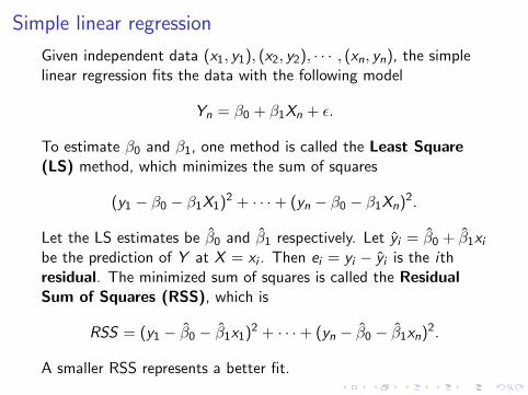
Given independent data (x1, y1), (x2, y2), · · · , (xn, yn), the simplelinear regression fits the data with the following model

Yn = β0 + β1Xn + ε.

To estimate β0 and β1, one method is called the Least Square(LS) method, which minimizes the sum of squares

(y1 − β0 − β1X1)2 + · · ·+ (yn − β0 − β1Xn)2.

Let the LS estimates be β0 and β1 respectively. Let yi = β0 + β1xibe the prediction of Y at X = xi . Then ei = yi − yi is the ithresidual. The minimized sum of squares is called the ResidualSum of Squares (RSS), which is

RSS = (y1 − β0 − β1x1)2 + · · ·+ (yn − β0 − β1xn)2.

A smaller RSS represents a better fit.

0 50 100 150 200 250 300

51

01

52

02

5

TV

Sa

les

Figure: For the Advertising data, the least squares fit for the regression ofsales onto TV is shown. The fit is found by minimizing the sum ofsquared errors. Each grey line segment represents an error, and the fitmakes a compromise by averaging their squares. In this case a linear fitcaptures the essence of the relationship, although it is somewhat deficientin the left of the plot. β0 = 7.03, β1 = 0.0475.

β0

β1

2.15

2.2

2.3

2.5

3

3

3

3

5 6 7 8 9

0.0

30.0

40.0

50.0

6

RS

S

β1

β0

Figure: Contour and three-dimensional plots of the RSS on theAdvertising data, using sales as the response and TV as the predictor.The red dots correspond to the least squares estimates β0 and β1.

Assessing accuracy of the coefficient estimates

−2 −1 0 1 2

−1

0−

50

51

0

X

Y

−2 −1 0 1 2

−1

0−

50

51

0

X

Y

Figure: A simulated data set. Left: The red line represents the truerelationship, f (X ) = 2 + 3X , which is known as the population regressionline. The blue line is the least squares line; it is the least squares estimatefor f (X ) based on the observed data, shown in black. Right: Thepopulation regression line is again shown in red, and the least squares linein dark blue. In light blue, ten least squares lines are shown, eachcomputed on the basis of a separate random set of observations. Eachleast squares line is different, but on average, the least squares lines arequite close to the population regression line.

Bias and Unbiasedness: The bias of an estimator means it mightover or under estimate the truth averaging the correspondingestimates for a large number of data sets. An unbiased estimatordoes not systematically over- or under-estimate the trueparameter. The property of unbiasedness holds for the leastsquares coefficient estimates.Standard error: The standard error of an estimator is standarddevition of the estimator, describing its varation due to repeatedsampleing. Denoted as SE (β0) and SE (β1).The 95% CIs for the true parameters β0 and β1 are

βi + /− 2SE (βi ), i = 0, 1.

Hypothesis testingNull hypothesis H0: There is no relationship between X and Y .Alternative hypothesis Ha: There is some relationship between Xand Y . This is mathematically equivalent to

H0 : β1 = 0 Ha : β1 6= 0.

Test statistic: t = β1SE(β1)

.

Null distribution: The distribution of the test statistic under H0.The above defined t statistic follows a t distribution with n − 2degree of freedom.P-value: the probability of observing any value equal to |t| orlarger, assuming β1 = 0, that is, p-value=P(T > |t||H0). A smallp-value indicates that it is unlikely to observe such a substantialassociation between the predictor and the response due to chance,in the absence of any real association between the predictor andthe response. Hence, if we see a small p-value, then we can inferthat there is an association between the predictor and the response.We reject the null hypothesis-that is, we declare a relationship toexist between X and Y -if the p-value is small enough.

Coefficient Std. error t-statistic p-value

Intercept 7.0325 0.4578 15.36 < 0.0001TV 0.0475 0.0027 17.67 < 0.0001

Table: For the Advertising data, coefficients of the least squares modelfor the regression of number of units sold on TV advertising budget. Anincrease of $1,000 in the TV advertising budget is associated with anincrease in sales by around 50 units (Recall that the sales variable is inthousands of units, and the TV variable is in thousands of dollars).

Assessing model fitResidual standard error (RSE): Roughly speaking, it is theaverage amount that the response will deviate from the trueregression line.

RSE =

√RSS

n − 2.

R2:measures the proportion of variability in Y that can beexplained using X . An R2 statistic that is close to 1 indicates thata large proportion of the variability in the response has beenexplained by the regression. A number near 0 indicates that theregression did not explain much of the variability in the response;this might occur because the linear model is wrong, or the inherenterror σ2 is high, or both.

R2 = 1− RSS

TSS, where TSS =

2∑i=1

(yi − y)2.

For simple linear regression, R2 = r2 where r is the Pearsoncorrelation coefficient between X and Y .

Quantity Value

Residual standard error 3.26R2 0.612

Table: For the Advertising data, more information about the leastsquares model for the regression of number of units sold on TVadvertising budget.

Multiple linear regression

Y = β0 + β1X1 + · · ·+ βpXp + ε.

LS Estimates of the coefficients: Choose β0, β1, · · · , βp tominimize

RSS =n∑

i=1

(yi − β0 − β1xi1 − β2xi2 − · · · − βpxip)2.

Coefficient Std. error t-statistic p-valueIntercept 7.0325 0.4578 15.36 < 0.0001

TV 0.0475 0.0027 17.67 < 0.0001

Coefficient Std. error t-statistic p-valueIntercept 9.312 0.563 16.54 < 0.0001

radio 0.203 0.020 9.92 < 0.0001

Coefficient Std. error t-statistic p-valueIntercept 12.351 0.621 19.88 < 0.0001

newspaper 0.055 0.017 3.30 < 0.0001

Coefficient Std. error t-statistic p-valueIntercept 2.939 0.3119 9.42 < 0.0001

TV 0.046 0.0014 32.81 < 0.0001radio 0.189 0.0086 21.89 < 0.0001

newspaper -0.001 0.0059 −0.18 0.8599

cor(TV, radio)=0.0548, cor(TV, newspaper)=0.0567, cor(radio,newspaper)=0.3541.

Test the hypothesis

H0 : β1 = · · · = βp = 0 Ha : at least one of βj is non-zero.

Test statistic: F = (TSS−RSS)/pRSS/(n−p−1) .

Null distribution: the test statistic follows the F distribution with pand n − p − 1 degrees of freedom.

Quantity Value

Residual standard error 1.69R2 0.897

F -statistic 570

Table: More information about the least squares model for the regressionof number of units sold on TV, newspaper, and radio advertising budgetsin the Advertising data.

Test the hypothesis

H0 : βp−q+1 = · · · = βp = 0 Ha : H0 is not true.

Test statistic: F = (RSS0−RSS)/qRSS/(n−p−1) , where RSS0 is the residual sum of

squares of the model that uses all the variables except those last q.Null distribution: the test statistic follows the F distribution with qand n − p − 1 degrees of freedom.Multiple testing:Given these individual p-values for each variable,why do we need to look at the overall F-statistic? After all, itseems likely that if any one of the p-values for the individualvariables is very small, then at least one of the predictors is relatedto the response.

Deciding on important variablesTotal model space: 2p models.Model comparison criteria: Mallow’s Cp, Akaike informationcriterion (AIC), Bayesian information criterion (BIC), and adjustedR2.Three classical approaches:

I Forward selection. We begin with the null model-a modelthat contains an intercept but no predictors. We then fit psimple linear regressions and add to the null model thevariable that results in the lowest RSS. We then add to thatmodel the variable that resultsin the lowest RSS for the newtwo-variable model. This approach is continued until somestopping rule is satisfied.

I Backward selection. We start with all variables in themodel, and remove the variable with the largest p-value-thatis, the variable that is the least statistically significant. Thenew (p − 1)-variable model is fit, and the variable with thelargest p-value is removed. This procedure continues until astopping rule is reached.

I

I Mixed selection. This is a combination of forward andbackward selection. We start with no variables in the model,and as with forward selection, we add the variable thatprovides the best fit. We continue to add variablesone-by-one. Of course, as we noted with the Advertisingexample, the p-values for variables can become larger as newpredictors are added to the model. Hence, if at any point thep-value for one of the variables in the model rises above acertain threshold, then we remove that variable from themodel. We continue to perform these forward and backwardsteps until all variables in the model have a sufficiently lowp-value, and all variables outside the model would have a largep-value if added to the model.

Assessing model fit: RSE =√RSS/(n − p − 1) and R2 as

defined before.Prediction: We use both y0 = β0 + β1x01 + · · ·+ βpx0p toestimate the regression line (the average value of the response) atx0 = (x01, x02, · · · , x0p) and predict the actual response at x0. Butthe estimation confidence interval and the prediction interval aredifferent. For example, for the advertisement data, given that$100,000 is spent on TV advertising and $20,000 is spent on radioadvertising in each city, the 95 % confidence interval is [10,985,11,528], and the 95 % prediction interval is [7,930, 14,580]. Thelatter is wider because of the irreducible error.

Qualitative predictorsQualitative predictors, also called factors, discrete/categoricalvariables, are variables that take countable (in practice, a few)number of values, for example, gender and ethnicity.Levels of qualitative predictors: Possible values of the predictorsDummy variables: coding of the predictors to use in regression0-1 coding for two level predictors:

xi =

{1 if the ith person is female0 if the ith person is male

yi = β0 + β1xi + εi =

{β0 + β1 + εi if the ith person is femaleβ0 + εi if the ith person is male

Coefficient Std. error t-statistic p-value

Intercept 509.80 33.13 15.389 < 0.0001gender[Female] 19.73 46.05 0.429 0.6690

Table: Least squares coefficient estimates associated with the regressionof balance onto gender in the Credit data set.

Sum to zero contrast for two level predictors

:

xi =

{1 if the ith person is female−1 if the ith person is male

yi = β0 + β1xi + εi =

{β0 + β1 + εi if the ith person is femaleβ0 − β1 + εi if the ith person is male

Coefficient Std. error t-statistic p-value

Intercept 519.665 23.026 22.569 < 0.0001gender1 9.865 23.026 0.429 0.6690

Table: Least squares coefficient estimates associated with the regressionof balance onto gender in the Credit data set.

Qualitative factors with multiple levelsFor example, ethnicity in the credit data set has three levels:Asian, Caucasian, and African American.Coding with multiple 0-1 dummy variables:

xi1 =

{1 if the ith person is Asian0 if the ith person is not Asian

xi2 =

{1 if the ith person is Caucasion0 if the ith person is not Caucasion

Regression with multiple level factors:

yi = β0+β1xi1+β2xi2+εi =

β0 + β1 + εi if the ith person is Asianβ0 − β2 + εi if the ith person is Caucasianβ0 + εi if the ith person is African American

where β0 is called the baseline.

Coefficient Std. error t-statistic p-valueIntercept 531.00 46.32 11.464 < 0.0001

ethnicity[Asian] -18.69 65.02 -0.287 0.7740ethnicity[Caucasian] -12.50 56.68 -0.221 0.8260

Table: Least squares coefficient estimates associated with the regressionof balance onto ethnicity in the Credit data set.

To test whehter ethnicity is a significant predictor, need to test β1and β2 simultaneously:

H0 : β1 = β2 = 0 H1 : H0 is not true.

Use F test for the above hopothesis. The F -test has a p-value of0.96, indicating that we cannot reject the null hypothesis thatthere is no relationship between balance and ethnicity.

Removing additive assumptions/adding interactions

Suppose that spending money on radio advertising actuallyincreases the effectiveness of TV advertising, so that the slopeterm for TV should increase as radio increases. In this situation,given a fixed budget of $100,000, spending half on radio and halfon TV may increase sales more than allocating the entire amountto either TV or to radio. In marketing, this is known as a synergyeffect, and in statistics it is referred to as an interaction effect.See the following interaction plot.

> library(rgl)

> plot3d(Ad$TV, Ad$Radio, Ad$Sales)

> planes3d(1, 1, 0, -100, color="red")

Linear regression with interactions

Yi = β0 + β1X1i + β2X2i + β3X1iX2i + εi .

Coefficient Std. error t-statistic p-valueIntercept 6.7502 0.248 27.23 < 0.0001

TV 0.0191 0.002 12.70 < 0.0001radio 0.0289 0.009 3.24 0.0014

TVXradio 0.0011 0.000 20.73 < 0.0001

Table: For the Advertising data, least squares coefficient estimatesassociated with the regression of sales onto TV and radio, with aninteraction term.

I The R2 for the model is 96.8 %, compared to only 89.7 % for themodel that predicts sales using TV and radio without an interactionterm. This means that (96.8 - 89.7)/(100 - 89.7) = 69 % of thevariability in sales that remains after fitting the additive model hasbeen explained by the interaction term.

I an increase in TV advertising of $1,000 is associated with increasedsales of (β1 + β3Xradio)X 1,000 = 19+1.1 X radio units. And anincrease in radio advertising of $1,000 will be associated with anincrease in sales of (β2 + β3 X TV) X 1,000 = 29 + 1.1 X TV units.

I The hierarchical principle states that if we include an interactionin a model, we should also include the main effects, even if thep-values associated with their coefficients are not significant.

Non-linear relationship

50 100 150 200

10

20

30

40

50

Horsepower

Mile

s p

er

ga

llon

Linear

Degree 2

Degree 5

Figure: The Auto data set. For a number of cars, mpg and horsepowerare shown. The linear regression fit is shown in orange. The linearregression fit for a model that includes horsepower2 is shown as a bluecurve. The linear regression fit for a model that includes all polynomialsof horsepower up to fifth-degree is shown in green.

Coefficient Std. error t-statistic p-value

Intercept 56.9001 1.8004 31.6 < 0.0001horsepower -0.4662 0.0311 -15.0 < 0.0001horsepower2 0.0012 0.0001 10.1 < 0.0001

Table: For the Auto data set, least squares coefficient estimatesassociated with the regression of mpg onto horsepower and horsepower2.

Potential problems

I Non-linearity of the response-predictor relationships.

I Correlation of error terms.

I Non-constant variance of error terms.

I Outliers.

I High-leverage points.

I Collinearity.

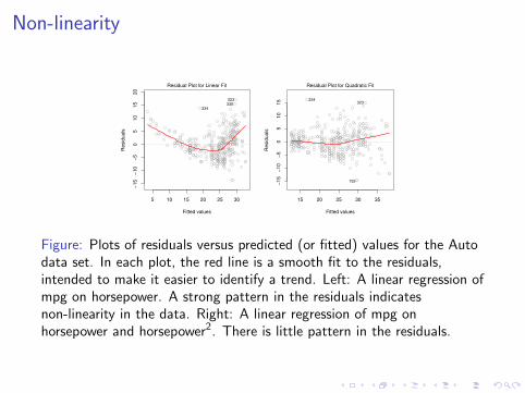
Non-linearity

5 10 15 20 25 30

−15

−10

−5

05

10

15

20

Fitted values

Resid

uals

Residual Plot for Linear Fit

323

330

334

15 20 25 30 35

−15

−10

−5

05

10

15

Fitted values

Resid

uals

Residual Plot for Quadratic Fit

334323

155

Figure: Plots of residuals versus predicted (or fitted) values for the Autodata set. In each plot, the red line is a smooth fit to the residuals,intended to make it easier to identify a trend. Left: A linear regression ofmpg on horsepower. A strong pattern in the residuals indicatesnon-linearity in the data. Right: A linear regression of mpg onhorsepower and horsepower2. There is little pattern in the residuals.

If the residual plot indicates that there are non-linear associationsin the data, then a simple approach is to use non-lineartransformations of the predictors, such as log(X ),

√X , and X 2, in

the regression model. In the later chapters of this book, we willdiscuss other more advanced non-linear approaches for addressingthis issue.

Correlation of error terms

0 20 40 60 80 100

−3

−1

01

23

ρ=0.0

Re

sid

ua

l

0 20 40 60 80 100

−4

−2

01

2ρ=0.5

Re

sid

ua

l

0 20 40 60 80 100

−1

.5−

0.5

0.5

1.5

ρ=0.9

Re

sid

ua

l

Observation

Figure: Plots of residuals from simulated time series data sets generatedwith differing levels of correlation ρ between error terms for adjacent timepoints.

If in fact there is correlation among the error terms, then theestimated standard errors will tend to underestimate the truestandard errors. As a result, confidence and prediction intervals willbe narrower than they should be. Then we may have anunwarranted sense of confidence in our model.Remedies include time series analysis, linear mixed effects models,etc. This topic is not discussed in this course.

Non-constant variance of error terms/heteroscedasticity

10 15 20 25 30

−10

−5

05

10

15

Fitted values

Resid

uals

Response Y

998

975845

2.4 2.6 2.8 3.0 3.2 3.4

−0.8

−0.6

−0.4

−0.2

0.0

0.2

0.4

Fitted values

Resid

uals

Response log(Y)

437671

605

Figure: Residual plots. In each plot, the red line is a smooth fit to theresiduals, intended to make it easier to identify a trend. The blue linestrack the outer quantiles of the residuals, and emphasize patterns. Left:The funnel shape indicates heteroscedasticity. Right: The predictor hasbeen log-transformed, and there is now no evidence of heteroscedasticity.

one possible solution is to transform the response Y using aconcave function such as log(Y ) or

√Y . Such a transformation

results in a greater amount of shrinkage of the larger responses,leading to a reduction in heteroscedasticity.Sometimes we have a good idea of the variance of each response.For example, the ith response could be an average of ni rawobservations. If each of these raw observations is uncorrelated withvariance σ2, then their average has variance σ2i = σ2/ni . In thiscase a simple remedy is to fit our model by weighted least squares,with weights proportional to the inverse weighted variances-i.e.wi = ni in this case.

Outliers

−2 −1 0 1 2

−4

−2

02

46

20

−2 0 2 4 6

−1

01

23

4

Fitted Values

Resid

uals

20

−2 0 2 4 6

02

46

Fitted Values

Stu

dentized R

esid

uals

20

X

Y

Figure: Left: The least squares regression line is shown in red, and theregression line after removing the outlier is shown in blue. Center: Theresidual plot clearly identifies the outlier. Right: The outlier has astudentized residual of 6; typically we expect values between ???3 and 3.

It is typical for an outlier that does not have an unusual predictorvalue to have little effect on the least squares fit. However, even ifan outlier does not have much effect on the least squares fit, it cancause other problems. For instance, inclusion of the outlier causesthe R2 to decline from 0.892 to 0.805.If we believe that an outlier has occurred due to an error in datacollection or recording, then one solution is to simply remove theobservation. However, care should be taken, since an outlier mayinstead indicate a deficiency with the model, such as a missingpredictor.

High leverage points

−2 −1 0 1 2 3 4

05

10

20

41

−2 −1 0 1 2

−2

−1

01

2

0.00 0.05 0.10 0.15 0.20 0.25

−1

01

23

45

Leverage

Stu

de

ntize

d R

esid

ua

ls

20

41

X

Y

X1

X2

Figure: Left: Observation 41 is a high leverage point, while 20 is not.The red line is the fit to all the data, and the blue line is the fit withobservation 41 removed. Center: The red observation is not unusual interms of its X1 value or its X2 value, but still falls outside the bulk of thedata, and hence has high leverage. Right: Observation 41 has a highleverage and a high residual.

Observation 41 stands out as having a very high leverage statistic as wellas a high studentized residual. This is a particularly dangerouscombination! This plot also reveals the reason that observation 20 hadrelatively little effect on the least squares fit: it has low leverage.

In order to quantify an observation’s leverage, we compute theleverage statistic. A large value of this statistic indicates anobservation with high leverage leverage. For a simple linearregression,

hi =1

n+

xi − x∑ni=1(xi − x)2

.

The leverage statistic hi is always between 1/n and 1, and theaverage leverage for all the observations is always equal to(p + 1)/n. So if a given observation has a leverage statistic thatgreatly exceeds (p+1)/n, then we may suspect that thecorresponding point has high leverage.There is a simple extension of hi to the case of multiple predictors,which is even more useful as identification of high leverage pointsin this case cannot be done visually.

Colinearity

21.25

21.5

21.8

0.16 0.17 0.18 0.19

−5

−4

−3

−2

−1

0

21.5

21.8

−0.1 0.0 0.1 0.2

01

23

45

βLimitβLimit

βAge

βRating

Figure: Contour plots for the RSS values as a function of the parametersβ for various regressions involving the Credit data set. In each plot, theblack dots represent the coefficient values corresponding to the minimumRSS . Left: A contour plot of RSS for the regression of balance onto ageand limit. The minimum value is well defined. Right: A contour plot ofRSS for the regression of balance onto rating and limit. Because of thecollinearity, there are many pairs (βLimit , βRating ) with a similar value forRSS .

Coefficient Std. error t-statistic p-value

Intercept -173.411 43.828 -3.957 < 0.0001Model 1 age -2.292 0.672 -3.407 0.0007

limit 0.173 0.005 34.496 < 0.0001

Intercept -377.537 45.254 -8.343 < 0.0001Model 2 rating 2.202 0.952 2.312 0.0213

limit 0.025 0.064 0.384 0.7012

Table: The results for two multiple regression models involving the Creditdata set are shown. Model 1 is a regression of balance on age and limit,and Model 2 a regression of balance on rating and limit. The standarderror of βlimit increases 12-fold in the second regression, due tocollinearity.

Since collinearity reduces the accuracy of the estimates of theregression coefficients, it causes the standard error for βlimit togrow. This means that the power of the hypothesis test-theprobability of correctly detecting a non-zero coefficient-is reducedby collinearity.A simple way to detect collinearity is to look at the correlationmatrix of the predictors.Unfortunately, not all collinearity problems can be detected byinspection of the correlation matrix: it is possible for collinearity toexist between three or more variables even if no pair of variableshas a particularly high correlation. We call this situationmulticollinearity.

variance inflation factor (VIF): the ratio of the variance of βjwhen fitting the full model divided by the variance of βj if fit on itsown. The formula reduces to

VIF (βj) =1

1− R2Xj |X−j

where R2Xj |X−j

is the R2 from a regression of Xj onto all of the

other predictors.As a rule of thumb, a VIF value that exceeds 5 or 10 indicates aproblematic amount of colinearity.In the Credit data, a regression of balance on age, rating, and limitindicates that the predictors have VIF values of 1.01, 160.67, and160.59. As we suspected, there is considerable collinearity in thedata!

Two simple solutions: 1. drop one of the problematic variablesfrom the regression. For instance, if we regress balance onto ageand limit, without the rating predictor, then the resulting VIFvalues are close to the minimum possible value of 1, and the R2

drops from 0.754 to 0.75. So dropping rating from the set ofpredictors has effectively solved the collinearity problem withoutcompromising the fit.2. combine the collinear variables together into a single predictor.

K-Nearest Neighbor regression

yy

x1x1

x 2x 2

Figure: Plots of f (X ) using KNN regression on a two-dimensional dataset with 64 observations (orange dots). Left: K = 1 results in a roughstep function fit. Right: K = 9 produces a much smoother fit. KNNestimate: f (x0) = 1

N

∑xi∈N0

yi .

−1.0 −0.5 0.0 0.5 1.0

12

34

−1.0 −0.5 0.0 0.5 1.0

12

34

yy

xx

Figure: Plots of f (X ) using KNN regression on a one-dimensional dataset with 100 observations. The true relationship is given by the blacksolid line. Left: The blue curve corresponds to K = 1 and interpolates(i.e. passes directly through) the training data. Right: The blue curvecorresponds to K = 9, and represents a smoother fit.

−1.0 −0.5 0.0 0.5 1.0

12

34

0.2 0.5 1.0

0.0

00.0

50.1

00.1

5

Mean S

quare

d E

rror

y

x 1/K

Figure: Left: The blue dashed line is the least squares fit to the data.Since f (X ) is in fact linear (displayed as the black line), the least squaresregression line provides a very good estimate of f (X ). Right: The dashedhorizontal line represents the least squares test set MSE , while the greensolid line corresponds to the MSE for KNN as a function of 1/K (on thelog scale). Linear regression achieves a lower test MSE than does KNNregression, since f (X ) is in fact linear. For KNN regression, the bestresults occur with a very large value of K , corresponding to a small valueof 1/K .

−1.0 −0.5 0.0 0.5 1.0

0.5

1.0

1.5

2.0

2.5

3.0

3.5

0.2 0.5 1.0

0.0

00

.02

0.0

40

.06

0.0

8

Me

an

Sq

ua

red

Err

or

−1.0 −0.5 0.0 0.5 1.0

1.0

1.5

2.0

2.5

3.0

3.5

0.2 0.5 1.0

0.0

00

.05

0.1

00

.15

Me

an

Sq

ua

red

Err

or

yy

x

x

1/K

1/K

Figure: Top Left: In a setting with a slightly non-linear relationshipbetween X and Y (solid black line), the KNN fits with K = 1 (blue) andK = 9 (red) are displayed. Top Right: For the slightly non-linear data,the test set MSE for least squares regression (horizontal black) and KNNwith various values of 1/K (green) are displayed. Bottom Left andBottom Right: As in the top panel, but with a strongly non-linearrelationship between X and Y .

Curse of dimensionality

0.2 0.5 1.0

0.0

0.2

0.4

0.6

0.8

1.0

p=1

0.2 0.5 1.0

0.0

0.2

0.4

0.6

0.8

1.0

p=2

0.2 0.5 1.0

0.0

0.2

0.4

0.6

0.8

1.0

p=3

0.2 0.5 1.0

0.0

0.2

0.4

0.6

0.8

1.0

p=4

0.2 0.5 1.0

0.0

0.2

0.4

0.6

0.8

1.0

p=10

0.2 0.5 1.0

0.0

0.2

0.4

0.6

0.8

1.0

p=20

Mean S

quare

d E

rror

1/K

Figure: Test MSE for linear regression (black dashed lines) and KNN(green curves) as the number of variables p increases. The true functionis non- linear in the first variable, and does not depend on the additionalvariables. The performance of linear regression deteriorates slowly in thepresence of these additional noise variables, whereas KNN’s performancedegrades much more quickly as p increases.

As a general rule, parametric methods will tend to outperformnon-parametric approaches when there is a small number ofobservations per predictor.Even in problems in which the dimension is small, we might preferlinear regression to KNN from an interpretability standpoint. If thetest MSE of KNN is only slightly lower than that of linearregression, we might be willing to forego a little bit of predictionaccuracy for the sake of a simple model that can be described interms of just a few coefficients, and for which p-values areavailable.