Introduction to SEXTANTE (v0.7)gvsigce.sourceforge.net/.../IntroductionToSEXTANTE.pdf ·...

Introduction to SEXTANTE (v0.7)

Vıctor OlayaEdition 1.0 — Rev. July 14, 2011

ii

An introduction to SEXTANTECopyright c©2010 Victor Olaya

Edicion 1.0Rev. July 14, 2011

Permision is granted to copy, distribute and modify this work according to the terms of the CreativeCommon Attritution license under which it is distributed. More information can be found at http:

//www.creativecommons.org. License applies to the text, as well as to the images created by theauthor, which are all the ones contained in this text except when otherwise stated.

This text can be downloaded in several formats, including editable ones, at http://www.sextantegis.com.

http://www.creativecommons.org

http://www.creativecommons.org

http://www.sextantegis.com

http://www.sextantegis.com

Contents

1 Introduction 1

1.1 Introduction . . . . . . . . . . . . . . . . . . . . . . . . . . . . . . . . . . . . . . 1

1.2 Basic elements of the SEXTANTE GUI . . . . . . . . . . . . . . . . . . . . . . 1

2 The SEXTANTE toolbox 5

2.1 Introduction . . . . . . . . . . . . . . . . . . . . . . . . . . . . . . . . . . . . . . 5

2.2 The algorithm dialog . . . . . . . . . . . . . . . . . . . . . . . . . . . . . . . . . 6

2.2.1 The parameters tab . . . . . . . . . . . . . . . . . . . . . . . . . . . . . 7

2.2.2 The analysis region tab . . . . . . . . . . . . . . . . . . . . . . . . . . . 9

2.3 Data objects generated by SEXTANTE algorithms . . . . . . . . . . . . . . . . 11

2.4 Context help . . . . . . . . . . . . . . . . . . . . . . . . . . . . . . . . . . . . . 13

2.5 Configuring SEXTANTE . . . . . . . . . . . . . . . . . . . . . . . . . . . . . . . 15

2.5.1 General . . . . . . . . . . . . . . . . . . . . . . . . . . . . . . . . . . . . 15

2.5.2 Folders . . . . . . . . . . . . . . . . . . . . . . . . . . . . . . . . . . . . 16

2.5.3 Model . . . . . . . . . . . . . . . . . . . . . . . . . . . . . . . . . . . . . 16

2.5.4 GRASS, SAGA and other additional algorithm providers . . . . . . . . 16

2.6 Iterative execution of algorithms . . . . . . . . . . . . . . . . . . . . . . . . . . 16

3 The SEXTANTE graphical modeler 19

3.1 Introduction . . . . . . . . . . . . . . . . . . . . . . . . . . . . . . . . . . . . . . 19

3.2 Definition of inputs . . . . . . . . . . . . . . . . . . . . . . . . . . . . . . . . . . 20

3.3 Definition of the workflow . . . . . . . . . . . . . . . . . . . . . . . . . . . . . . 21

3.4 Editing the model . . . . . . . . . . . . . . . . . . . . . . . . . . . . . . . . . . 23

3.5 Saving and loading models . . . . . . . . . . . . . . . . . . . . . . . . . . . . . . 23

4 The SEXTANTE batch processing interface 25

4.1 Introduccion . . . . . . . . . . . . . . . . . . . . . . . . . . . . . . . . . . . . . . 25

4.2 The parameters table . . . . . . . . . . . . . . . . . . . . . . . . . . . . . . . . . 25

4.3 Filling the parameters table . . . . . . . . . . . . . . . . . . . . . . . . . . . . . 26

4.4 Setting the output region . . . . . . . . . . . . . . . . . . . . . . . . . . . . . . 28

4.5 Executing the batch process . . . . . . . . . . . . . . . . . . . . . . . . . . . . . 29

5 The SEXTANTE command–line interface 31

5.1 Introduction . . . . . . . . . . . . . . . . . . . . . . . . . . . . . . . . . . . . . . 31

5.2 The interface . . . . . . . . . . . . . . . . . . . . . . . . . . . . . . . . . . . . . 31

iii

iv CONTENTS

5.2.1 Getting information about data . . . . . . . . . . . . . . . . . . . . . . . 325.3 Getting information about algorithms . . . . . . . . . . . . . . . . . . . . . . . 335.4 Running an algorithm . . . . . . . . . . . . . . . . . . . . . . . . . . . . . . . . 345.5 Adjusting the analysis region . . . . . . . . . . . . . . . . . . . . . . . . . . . . 355.6 Managing layers from the command–line interface . . . . . . . . . . . . . . . . 365.7 Creating scripts and running them from the toolbox . . . . . . . . . . . . . . . 36

6 The SEXTANTE history manager 396.1 Introduction . . . . . . . . . . . . . . . . . . . . . . . . . . . . . . . . . . . . . . 39

7 Configuring algorithm providers 417.1 Introduction . . . . . . . . . . . . . . . . . . . . . . . . . . . . . . . . . . . . . . 417.2 Configuring SAGA . . . . . . . . . . . . . . . . . . . . . . . . . . . . . . . . . . 417.3 Configuring GRASS . . . . . . . . . . . . . . . . . . . . . . . . . . . . . . . . . 42

7.3.1 Usage notes and limitations . . . . . . . . . . . . . . . . . . . . . . . . . 43Message output from GRASS modules . . . . . . . . . . . . . . . . . . . 44Graphical interface . . . . . . . . . . . . . . . . . . . . . . . . . . . . . . 44Vector data exchange . . . . . . . . . . . . . . . . . . . . . . . . . . . . 44Raster data exchange . . . . . . . . . . . . . . . . . . . . . . . . . . . . 45Topology . . . . . . . . . . . . . . . . . . . . . . . . . . . . . . . . . . . 45The GRASS region . . . . . . . . . . . . . . . . . . . . . . . . . . . . . . 45

7.3.2 Windows notes . . . . . . . . . . . . . . . . . . . . . . . . . . . . . . . . 457.3.3 Notes on specific modules . . . . . . . . . . . . . . . . . . . . . . . . . . 46

r.colors(.stddev) . . . . . . . . . . . . . . . . . . . . . . . . . . . . . . . 46r.in/out.gdal . . . . . . . . . . . . . . . . . . . . . . . . . . . . . . . . . 46r.mapcalculator . . . . . . . . . . . . . . . . . . . . . . . . . . . . . . . . 46r.null . . . . . . . . . . . . . . . . . . . . . . . . . . . . . . . . . . . . . . 46v.in/out.ogr . . . . . . . . . . . . . . . . . . . . . . . . . . . . . . . . . . 46v.surf.bspline . . . . . . . . . . . . . . . . . . . . . . . . . . . . . . . . . 47v.surf.idw . . . . . . . . . . . . . . . . . . . . . . . . . . . . . . . . . . . 47v.to.3d . . . . . . . . . . . . . . . . . . . . . . . . . . . . . . . . . . . . . 47

7.3.4 Technical details . . . . . . . . . . . . . . . . . . . . . . . . . . . . . . . 47

Chapter 1

Introduction

1.1 Introduction

Welcome to this introduction to SEXTANTE. This text is targeted at those using geospatialalgorithms from the SEXTANTE library through the graphical elements also included in thelibrary.

SEXTANTE is integrated into some of the most popular Java desktop GIS, and using it isidentical no matter which GIS you are using. If you have a GIS application which incorporatesSEXTANTE as its analysis platform, then this manual is for you.

Particular information about SEXTANTE algorithms is not found in this text. The usershould refer to the context help system instead.

1.2 Basic elements of the SEXTANTE GUI

There are four basic elements in the SEXTANTE GUI, which are used to run SEXTANTEalgorithms for different purposes. Chosing one tool or another will depend on the kind ofanalysis that is to be performed and the particular characteristics of each user an project.

Depending on the implementation of the GIS application you are using, these elementscan be accesed through menu entries (usually under a menu group named “SEXTANTE”) ora toolbar like the one shown next.

• The SEXTANTE toolbox. The main element of the SEXTANTE GUI, it is used toexecute a single algorithm or run a batch process based on that algorithm.

1

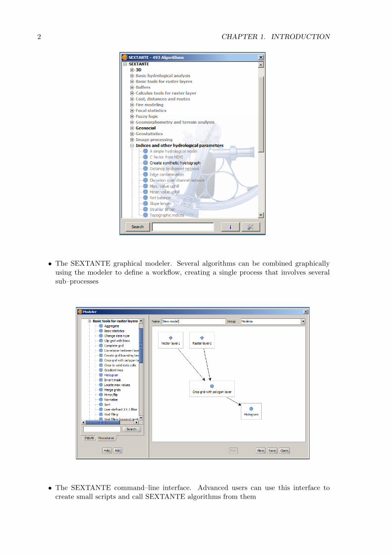
2 CHAPTER 1. INTRODUCTION

• The SEXTANTE graphical modeler. Several algorithms can be combined graphicallyusing the modeler to define a workflow, creating a single process that involves severalsub–processes

• The SEXTANTE command–line interface. Advanced users can use this interface tocreate small scripts and call SEXTANTE algorithms from them

1.2. BASIC ELEMENTS OF THE SEXTANTE GUI 3

• The SEXTANTE history manager. All actions performed using any of the aforemen-tioned elements are stored in a history file and can be later easily reproduced using thehistory manager

Along the following chapters we will review each one of this elements in detail.

4 CHAPTER 1. INTRODUCTION

Chapter 2

The SEXTANTE toolbox

2.1 Introduction

The Toolbox is the main element of the SEXTANTE GUI, and the one that you are more likelyto use in your daily work. It shows the list of all available algorithms grouped in differentblocks, and is the access point to run them whether as a single process or as a batch processinvolving several executions of a same algorithm on different sets of inputs.

Depending on the data available in the GIS, you will be able to execute an algorithm ornot. When there is enough data for the algorithm to be executed (i.e. the algorithm requiresraster layers and you have raster layer already loaded into the GIS), its name is shown inblack, otherwise, it is shown in grey.

In the lower part of the toolbox you can find a text box and a search button. To reducethe number of algorithms shown in the toolbox and make it easier to find the one you need,you can enter any word or phrase on the text box and click on the search button. SEXTANTE

5

6 CHAPTER 2. THE SEXTANTE TOOLBOX

will search the help files associated to each algorithm and show only those algorithms thatinclude the word or phrase in their corresponding help files. To show all the algorithms again,make a search with an empty string.

Notice that, as you type, the number of algorithms in the toolbox is reduced. A search isperformed as you type, but only on the algorithm names, not the hep files. You can use thisalso to quickly find and algorithm. In case you want to perform a full search and look for agiven word not just in the algorithm names but also in their associated help files, click theSearch button or hit the Enter key.

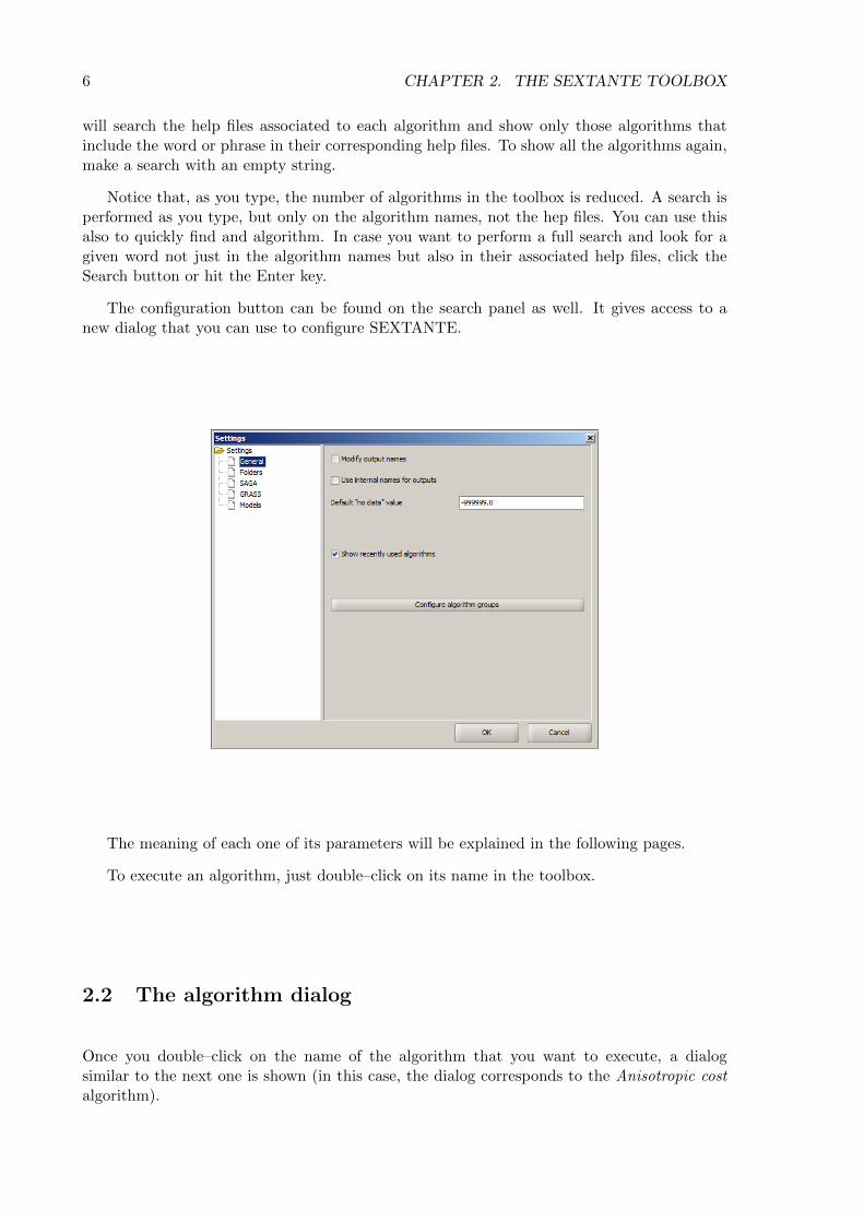
The configuration button can be found on the search panel as well. It gives access to anew dialog that you can use to configure SEXTANTE.

The meaning of each one of its parameters will be explained in the following pages.

To execute an algorithm, just double–click on its name in the toolbox.

2.2 The algorithm dialog

Once you double–click on the name of the algorithm that you want to execute, a dialogsimilar to the next one is shown (in this case, the dialog corresponds to the Anisotropic costalgorithm).

2.2. THE ALGORITHM DIALOG 7

This dialog is used to set the input values that the algorithm needs to be executed.

There is a main tab named Parameters where input values and configuration parametersare set. This tab has a different content depending on the requirements of the algorithm tobe executed, and is created automatically based on those requirements. On the left side, thename of the parameter is shown. On the right side the value of the parameter can be set.

Most algorithms have an additional tab named Output extent. This tab is used to definethe region that wants to be analyzed, in case you do not want to perform analysis on thewhole extent defined by the input layers. Also, it should be used to set the characteristics ofoutput raster layers, specifying its extent and its cell size.

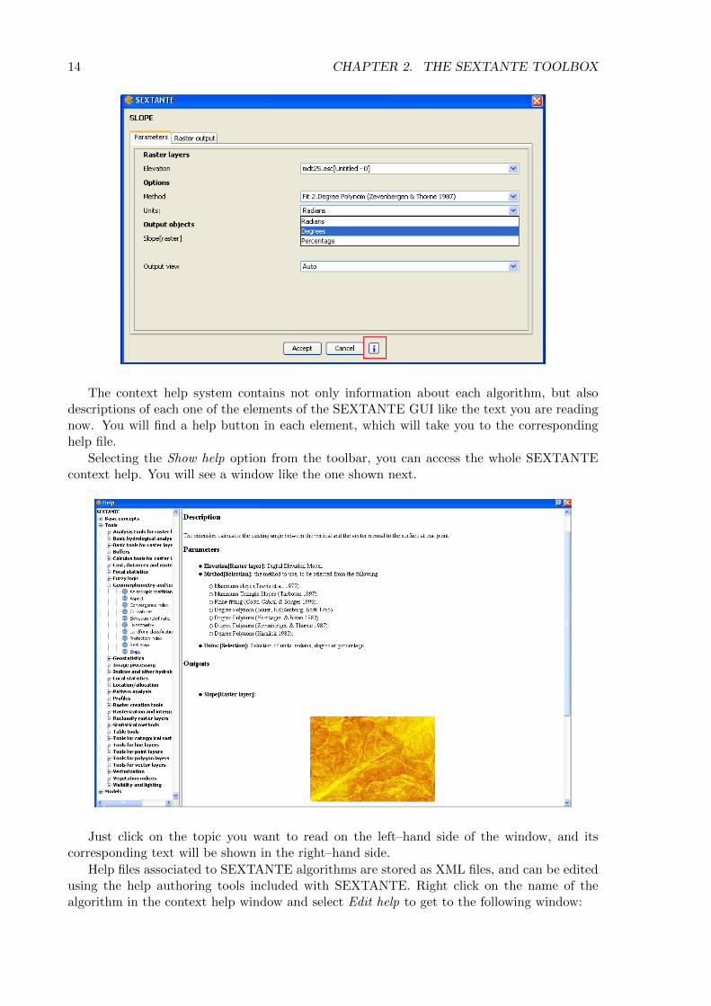
On the lower part of the window there is a help button. Click on it to see the context helprelated to the current algorithm, where you will find detailed description of each parameterand each output generated by the algorithm.

2.2.1 The parameters tab

Although the number and type of parameters depends on the characteristics of the algorithm,the structure is similar for all of them. The parameters found on the parameters tab can beof one of the following types.

• A raster layer, to select from a list of all the ones available in the GIS application

• A vector layer, to select from a list of all the ones available in the GIS application

• A table, to select from a list of all the ones available in the GIS application

• A method, to choose from a selection list of possible options

• A numerical value, to be introduced in a text box.

• A text string, to be introduced in a text box

• A field, to choose from the attributes table of a vector layer or a single table selected inanother parameter.

• A band, to select from the ones of a raster layer selected in another parameter. In boththis and the previous type of parameter, the list of possible choices depends on the valueselected in the parent parameter.


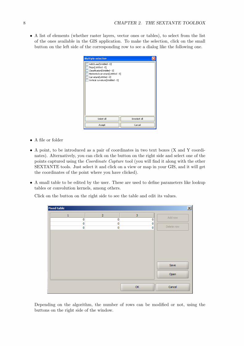
• A list of elements (whether raster layers, vector ones or tables), to select from the listof the ones available in the GIS application. To make the selection, click on the smallbutton on the left side of the corresponding row to see a dialog like the following one.

• A file or folder

• A point, to be introduced as a pair of coordinates in two text boxes (X and Y coordi-nates). Alternatively, you can click on the button on the right side and select one of thepoints captured using the Coordinate Capture tool (you will find it along with the otherSEXTANTE tools. Just select it and click on a view or map in your GIS, and it will getthe coordinates of the point where you have clicked).

• A small table to be edited by the user. These are used to define parameters like lookuptables or convolution kernels, among others.

Click on the button on the right side to see the table and edit its values.

Depending on the algorithm, the number of rows can be modified or not, using thebuttons on the right side of the window.

2.2. THE ALGORITHM DIALOG 9

If you have previously executed an algorithm (whether in this work session or in anotherone), you will find an additional component in the lower left part of the parameters tab.

By default, in this the parameters are set to the values they had in the last execution.Using the arrow buttons you can change to the values used in previous executions, browsingthe SEXTANTE history.

2.2.2 The analysis region tab

The Analysis region tab is found in those algorithms in which the user can select the extentof the region to be used for analysis. In most cases, this extent is also used to generate newlayers. This is particularly important in the case of raster layers, and in that case not onlythe extent is needed, but also a value for the cellsize.

Unlike in most GIS, when combining several raster layers as input for an algorithm, theydo not have to have the same extent and cellsize in order to process them together. Thatis, layers don’t have necessarily to “match” between them. Instead, the characteristics of theanalysis region (which are the ones used for the resulting raster layers, in case the algorithmgenerates such an output) are defined and SEXTANTE performs the corresponding resamplingand cropping needed to generate layer with those characteristics.

It is responsibility of the user to enter adequate values and be aware of the limitations ofthis mechanism, so as to generate cartographically sound results. (i.e. you can select a smallcell size for the resulting raster layers, but if the input layers you are using have a coarseresolution the results will not be geographically sound).

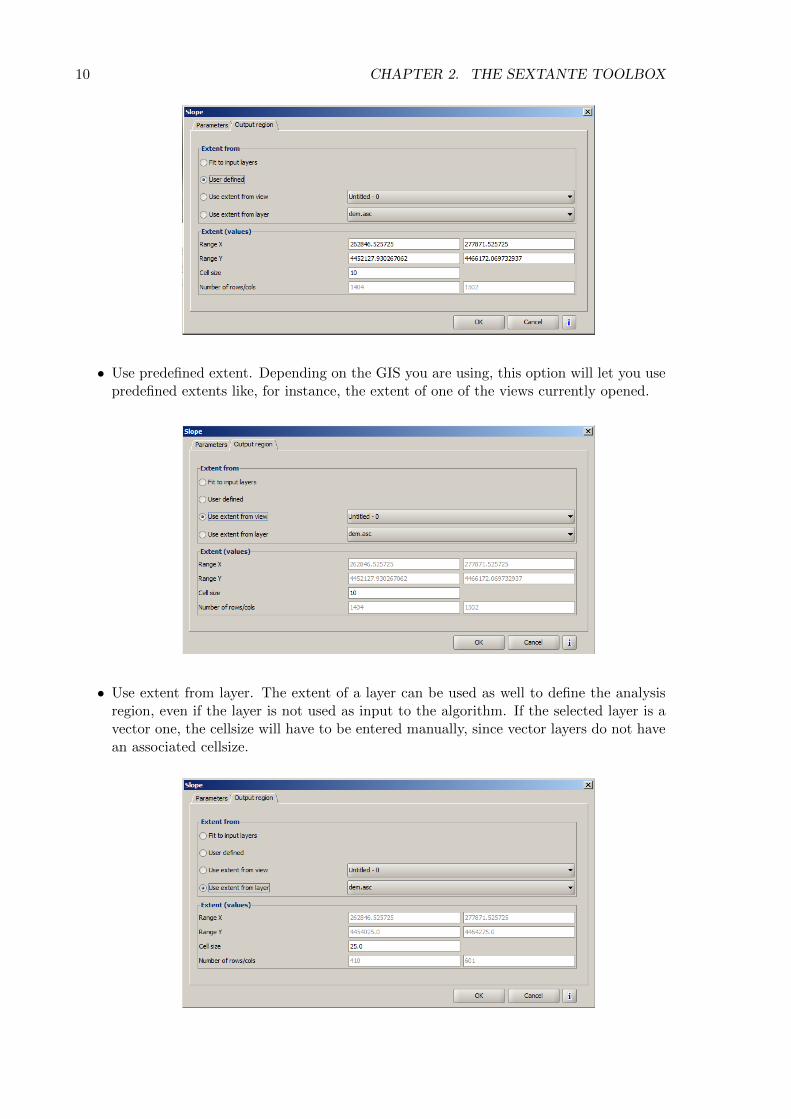
The following options are available in the Analysis region tab:

• Fit to input layers. By default, the extent is set based on the input layers. The minimumextent needed to cover all the input layers is used.

• User defined. The coordinates of the boundaries of the extent and the cellsize are bothdefined manually, entering the desired values in the corresponding text boxes. You willbe prompted to enter a cellsize always, no matter if the algorithm is just a vector one.Just ignore it and leave the default value, since the algorithm will not use it.


• Use predefined extent. Depending on the GIS you are using, this option will let you usepredefined extents like, for instance, the extent of one of the views currently opened.

• Use extent from layer. The extent of a layer can be used as well to define the analysisregion, even if the layer is not used as input to the algorithm. If the selected layer is avector one, the cellsize will have to be entered manually, since vector layers do not havean associated cellsize.

2.3. DATA OBJECTS GENERATED BY SEXTANTE ALGORITHMS 11

If an option other than the automatic fitting is selected, SEXTANTE will check that thevalues are correct and the resulting raster layers will not be too large (due to, for instance, awrong cell size). If the output layers seems to large, SEXTANTE will show the next messagedialog to ensure that the user really wants those layers to be created.

Not all algorithms have the first option available, since not all algorithms that generatelayers take some other similar layer as input. The interpolation algorithms, for instance, takea vector layer and create a raster one. The extent and cellsize of the latter has to be manuallydefined, since it cannot be set based solely on the input vector layer (vector layers do not havea cellsize value).

2.3 Data objects generated by SEXTANTE algorithms

Data objects generated by SEXTANTE can be of any of the following types:

• A raster layer

• A vector layer

• A table

• A graphical result (chart, graph, etc.)

• A text–only HTML–formatted result

Layers and tables can be saved, and the parameters window will contain a text box corre-sponding to each one of these outputs, where you can type the output channel to use for savingit. An output channel contains the information needed to save the resulting object somewhere.In the most usual case, you will save it to a file, but the architecture of SEXTANTE allowsfor any other way of storing it. For instance, a vector layer can be stored in a database oreven uploaded to a remote server using a WFS–T service. Although solutions like these arenot yet implemented, SEXTANTE can now easily handle them, and we expect to add newkinds of output channels in a near feature.

To select an output channel, just click on the button on the right side of the text box. Youwill see a dialog similar to the one shown next.


There are several tabs, each of them containing the elements needed to define a certainkind of output channel. Just go to the tab representing the one that you want and enter theinformation required. For instance, the File tab is just a file chooser where you have to selecta file or type its name. When you are done, click on the OK button.

The first tab you see contains two general options, with a button for each one:

• Save to temporary file

• Overwrite

Clicking on the “Save to temporary file” will cause SEXTANTE to select a temporaryfile for saving the resulting data object. That file will be deleted once you exit the GIS andSEXTANTE is shut down. This options should be used when you are executing an algorithmand want to use its results as intermediate data, but do not want to keep them permanently.

The “Overwrite” option will appear only on those algorithms that allow overwriting ofinput layers. In that case, the algorithm will replace the data of an input layer (the algorithmitself has to know which layer from all the input ones) instead of generating a new one. Awarning might be shown if the input layer cannot be overwritten (such as, for instance, a layeron a database that the user has no rights to edit). This option is currently only available forvector layers, and just in some algorithms were it makes sense.

Since file outputs are the most common ones, we will give some extra information aboutthem.

The format of the output is defined by the filename extension. The supported formatsdepend on the ones supported by the GIS onto which SEXTANTE is running. That meansthat SEXTANTE usually supports all the formats that the GIS is capable of writing. Toselect a format, just select the corresponding file extension. If the extension of the filepathyou entered does not match any of the supported ones, a default extension (usually dbf fortables, tif for raster layers and shp for vector ones) will be appended to the filepath and thefile format corresponding to that extension will be used to save the layer or table.

You can set a default folder for output data objects. Go to the configuration dialog (youcan open it from the toolbox), and in the “Folders” tab you will find a text box named “Output

2.4. CONTEXT HELP 13

folder”. This output folder is used as the default path in case you type just a filename withno path (i.e. myfile.shp) when executing an algorithm.

Sometimes, layers might have names that include special characters. For example, if yourasterize a layer named “mylayer”, the result will be a new layer named “mylayer[rasterized]”.Those brackets can cause you some problems if you later want to use that layer as input forthe raster calculator, or from the command–line interface, so it can be a good idea to removethem (the same happens with other characters such as “a” or “n” that might appear if you useSEXTANTE in spanish). You can tell SEXTANTE to automatically replace those characterwith valid standard ones. To do so, open the configuration dialog and select the “General”group. Select the check box with the label “Modify output names”.

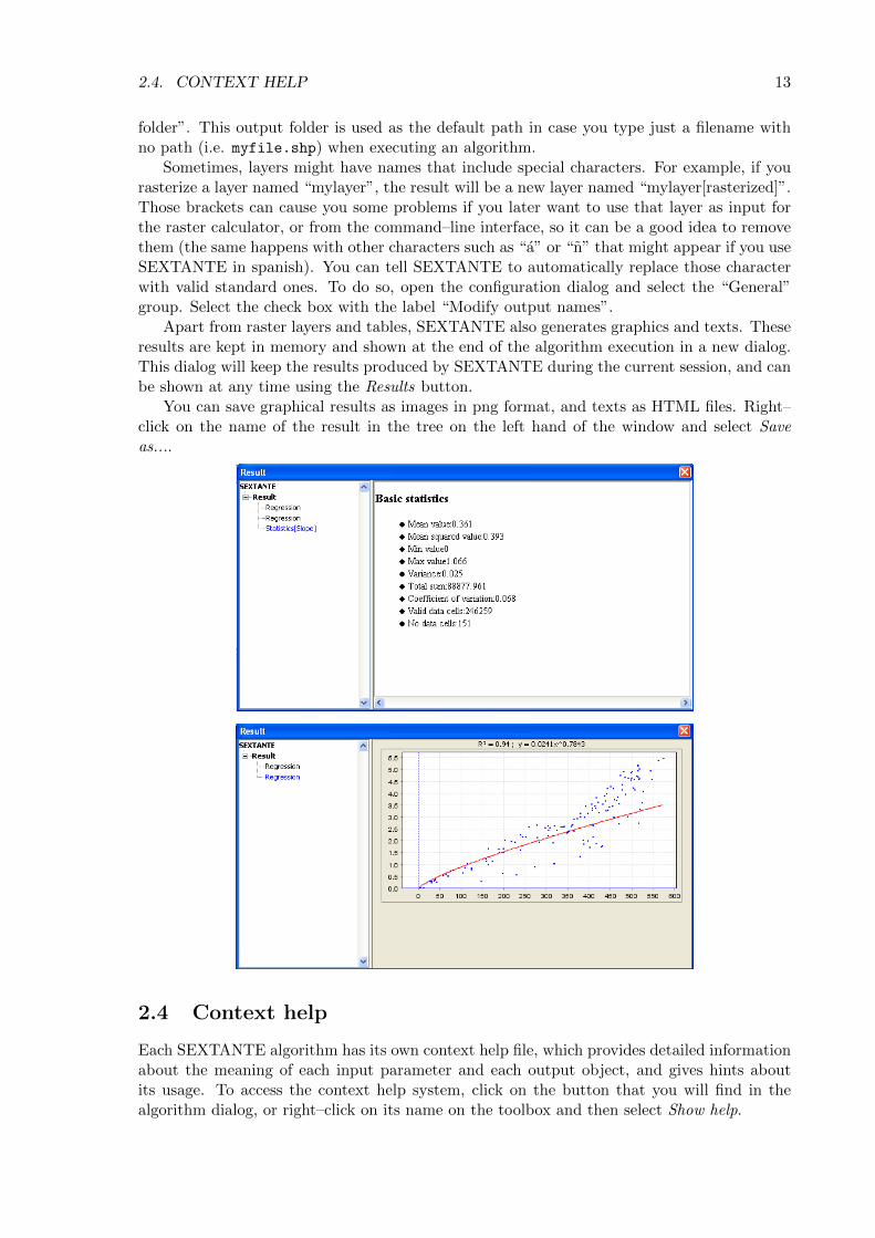
Apart from raster layers and tables, SEXTANTE also generates graphics and texts. Theseresults are kept in memory and shown at the end of the algorithm execution in a new dialog.This dialog will keep the results produced by SEXTANTE during the current session, and canbe shown at any time using the Results button.

You can save graphical results as images in png format, and texts as HTML files. Right–click on the name of the result in the tree on the left hand of the window and select Saveas....

2.4 Context help

Each SEXTANTE algorithm has its own context help file, which provides detailed informationabout the meaning of each input parameter and each output object, and gives hints aboutits usage. To access the context help system, click on the button that you will find in thealgorithm dialog, or right–click on its name on the toolbox and then select Show help.


The context help system contains not only information about each algorithm, but alsodescriptions of each one of the elements of the SEXTANTE GUI like the text you are readingnow. You will find a help button in each element, which will take you to the correspondinghelp file.

Selecting the Show help option from the toolbar, you can access the whole SEXTANTEcontext help. You will see a window like the one shown next.

Just click on the topic you want to read on the left–hand side of the window, and itscorresponding text will be shown in the right–hand side.

Help files associated to SEXTANTE algorithms are stored as XML files, and can be editedusing the help authoring tools included with SEXTANTE. Right click on the name of thealgorithm in the context help window and select Edit help to get to the following window:

2.5. CONFIGURING SEXTANTE 15

On the left–hand side you can select any of the elements to be documented (input param-eter and outputs, along with other fixed field such as a general description of the algorithm).Then use the right–hand side boxes to enter the text associated to that element or add images.

2.5 Configuring SEXTANTE

As we have seen, the configuration button in the lower part of the toolbox gives access to anew dialog where you can configure how SEXTANTE works. Configuration parameters arestructured in separate blocks that you can select on the left–hand side of the dialog.

2.5.1 General

You will see two check boxes in the upper part of this group:

• Modify output names: if you check this option, output names will be modified toavoid characters such as brackets, blank spaces or stress marks.

• Use internal names for outputs: when this option is selected, SEXTANTE usesinternal names to name output layers. This is useful if you plan to use the command–line interface to write scripts, since the names of the outputs can be know in advance(having a look at the help files, under the Command–line usage will inform you of thosenames). If this options is not selected, SEXTANTE will produce layers with names thatdepend on the current language or sometimes on the names of the input layers, whichcan cause you trouble if you plan to use those layers for your script.

Under that, you will two elements to configure the list of algorithms in the toolbox. Thefirst one can be used to remove the Most recently used group in the toolbox. Just uncheck thecheck box and you will not see that group.

The second one is a button that can be used to redefine how algorithms are organized inthe toolbox. Click on the button to get to the following dialog.


In it, you can change the group and subgroup each algorithm belongs to, and also you canselect whether to show or not a given algorithm. Type on the table cells to enter an alternativegroup of subgroup for an algorithm. Once you are done, click on the OK button. You canrestore the default groupings by clicking on the ”Restore default´´ button.

2.5.2 Folders

One folder can be defined:

• Output folder: when entering the filename for an output layer, if it does not includea valid path, it will be saved to this default output folder.

2.5.3 Model

The folder where models are stored has to be set in this field. This will be explained in detailin the following chapter. Once you have entered the path to the folder that you want to use,click on the button below to make SEXTANTE load all the models found there.

2.5.4 GRASS, SAGA and other additional algorithm providers

The set of algorithms of SEXTANTE can be extended by using additional algorithm providersthat wrap algorithms from a third–party software. SEXTANTE acts as a front–end to thoseapplications and can reuse their algorithms. Configuration of algorithm providers depends onthe characteristics of the provider itself and the software being called from SEXTANTE. Thisis explained in detail in a separate chapter at the end of this manual.

2.6 Iterative execution of algorithms

SEXTANTE algorithms can be executed iteratively when they include some kind of vectorinput. In this case, for a layer containing n features, the algorithm is executed n times, each

2.6. ITERATIVE EXECUTION OF ALGORITHMS 17

time taking an input layer that contains just one feature from the original layer.This is useful for certain processes, like, for instance, cropping a raster layer using a

vector layer with polygons. Given a polygon layer, the raster layer can be cropped in smallerones, each of them covering the minimum extent needed to include each one of the inputpolygons. This will require executing the corresponding algorithm as many times as polygonsare contained in the vector layer, which might be a long and tedious process. Instead, executingthe algorithm iteratively will automate the task, solving the problem in just one single step.

To execute an algorithm iteratively, right click on its name in the toolbox. You will seea new menu named Execute iteratively [parameter name]. There will be as many menus asvector layers the algorithm takes. You can only iterate over one of them, so you have to selectthe right one depending on what you want to do.

Clicking on the chosen menu, the usual algorithm dialog is shown. It is exactly like thedialog you would see if executing the algorithm the usual way. Just fill in the parametervalues and click on OK. The progress dialog will inform you of the step that is currently beingexecuted. Resulting layers will be added to the GIS GUI as usual.

When executing iteratively an algorithm that produces text output with numerical values(such as, for instance, statistics of a raster layer), it might be convenient to present those resultsin a different manner. Otherwise, combining a large number of such text outputs would bedifficult and not practical. For this reason, when an algorithms is executed iteratively, itsnumerical outputs (in case the algorithm generates them) are presented in a table in theresults manager. Each row of the table represents an execution of the algorithm, while eachcolumn contains the values of one of the numerical variables being calculated.

The following picture shows an example of one of such tables.

Chapter 3

The SEXTANTE graphical modeler

3.1 Introduction

The graphical modeler allows to create complex models using a simple and easy–to–use inter-face. When working with a GIS, most analysis operations are not isolated, but part of a chainof operations instead. Using the graphical modeler, that chain of processes can be wrappedinto a single process, so it is easier and more convenient to execute than a single process lateron a different set on inputs. No matter how many steps and different algorithms it involves,a model is executed as a single algorithm, thus saving time and effort, specially for largermodels.

The modeler has a working canvas where the structure of the model and the workflow itrepresents are shown. On the left part of the window, a panel with two tabs can be used toadd new elements to the model.

Creating a model is a two–step process.

• Definition of necessary inputs. These inputs will be added to the parameters window, sothe user can set their values when executing the model. The model itself is a SEXTANTE

19

20 CHAPTER 3. THE SEXTANTE GRAPHICAL MODELER

algorithm, so the parameters window is generated automatically as it happens with allthe algorithms included in the library.

• Definition of the workflow. Using the input data of the model, the workflow is definedadding algorithms and selecting how they use those inputs or the outputs generated byother algorithms already in the model

3.2 Definition of inputs

The first step to create a model is to define the inputs it needs. The following elements arefound in the Inputs tabs on the left side of the modeler window:

• Band

• Raster layer

• Vector layer

• String

• Table field

• Coordinate (Point)

• Table

• Fixed table

• Multiple input

• Selection

• Numerical value

• Boolean value

Double–clicking on any of them, a dialog is shown to define its caracteristics. Dependingon the parameter itself, the dialog will contain just one basic element (the description, whichis what the user will see when executing the model) or more of them. For instance, whenadding a numerical value, as can be seen in the next figure, apart from the description of theparameter is needed to set a default value, the type of numerical value and a range of validvalues.

For each added input, a new element is added to the modeler canvas.

3.3. DEFINITION OF THE WORKFLOW 21

3.3 Definition of the workflow

Once the inputs have been defined, it is time to define the algorithms to apply on them.Algorithms can be found in the Processes tab, grouped much in the same way as they are inthe toolbox.

To add a process, double–click on its name. An execution dialog will appear, with acontent similar to the one found execution panel that SEXTANTE shows when executing thealgorithm from the toolbox.

Some differences exist, however, the main one being the absence of a raster ouput tab,even if the selected algorithm generates raster layers as output.

Instead of the textbox that was used to set the filepath for output layers and tables, acheckbox and a text box are found. If the layer generated by the algorithm is just a temporaryresult that will be used as the input of another algorithm and should not be kept as a final


result, the check box should be left unchecked. Checking it means that the result is a finalone, and you have to supply also a valid description for the output, which will be the one theuser will see when executing the model.

Selecting the value of each parameter is also a bit different, since there are importantedifferences between the context of the modeler and the toolbox one. Let’s see how to introducethe values for each type of parameter.

• Layers (raster and vector) and tables. They are selectend from a list, but in this case thepossible values are not the layers or tables currently loaded in the GIS, but the list ofmodel input or the corresponding type, or other layers or tables generated by algorithmsalready added to the model.

• Numerical values. Literal values can be introduced directly on the textbox. This textboxis a list that can be used to select any of the numerical value input of the model. Inthis case, the parameter will take the value introduced by the user when executing themodel.

• String. Like in the case of numerical values, literal strings can be typed, or an inputstring can be selected

• Points. Coordinates cannot be directly introduced. Use the list to select one of thecoordinate inputs of the model

• Bands. The number of bands of the parent layer cannot be known at design–time, so it isnot possible to show the list of available bands. Instead, a list with band numbers from 1to 250, as well as the band parameters of the model, is shown. At run–time, SEXTANTEwill check if the parent raster layer selected by the user has enough bands and the givenband has therefore a valid value, and if not it will generate an error message.

• Table field. Like in the previous case, the fields of the parent table or layer cannot beknown at design–time, since they depend of the selection of the user each time the modelis executed. To set the value for this parameter, type the name of a field directly in thetextbox, or use the list to select a table field input already added to the model. Thevalidity of the selected field will be checked by SEXTANTE at run–time

• Selection. The list contains in this case not only the available option from the algorithm,but also the selection inputs already added to the current model

Once all the parameter have been assigned valid values, click on OK and the algorithmwill be added to the canvas. It will be linked to all the other elements in the canvas, whetheralgorithms or inputs, which provide objects that are used as inputs for that algorithm.

3.4. EDITING THE MODEL 23

3.4 Editing the model

Once the model has been designed, it can be executed clicling on the Execute button. Theexecution window will have a parameters tab automatically created based on the requirementsof the model (the inputs added to it), just like it happens when a simple algorithm is executed.If any of the algorithms of the model generates raster layers, the Raster output tab will beadded to the window.

Elements can be dragged to a different position within the canvas, to change the way themodule structure is displayed and make it more clear and intuitive. Links between elementsare update automatically.

To change the parameters of any of the algorithms of a model, double–click on it to accesits parameters window.

To delete an element, right–click on it and select Delete. Only those elements that do nothave any other one depending on them can be deleted. If you try to delete an element thatcannot be deleted, SEXTANTE will show the following warning message.

3.5 Saving and loading models

Models can be saved to be executed or edited at a later time. Use the Save button to savethe current model and the Open model to open any model previously saved. Model are savedin an XML file with the .model extension.

Models saved on the models folder will appear in the toolbox in a group that you can setusing the boxes in the top of the modeler window. Type in the name of the model and thenselect a group from the drop–down list. The list contains all the names of the already existing


groups, and also an additional group named “Models”. If none of this group suits your needs,you can type a new name directly in that box, which is editable.

When the toolbox is invoked, SEXTANTE searches the models folder for files with .modelextension and loads the models they contain. Since a model is itself a SEXTANTE algorithm,it can be added to the toolbox just like any other algorithm.

The models folder can be set from the SEXTANTE toolbox, clicking the configurationbutton and then introducing the path to the folder in the corresponding field. Go to the“Folders” tab to find it.

Models loaded from the models folder appear not only in the toolbox, but also in the algo-rithms tree in the Processes tab of the modeler window. That means that you can incorporatea model as a part of a bigger model, just as you add any other algorithm. however, modelsare shown with a different icon, to make it easy to recognize them.

By default, the models folder is the same one as the folder where SEXTANTE help filesare located. This folder contains a small set of example models, that you can use to betterunderstand how the modeler works. Open them and study how they are constructed. You canalso check their associated help files. As it has been said, models are themselves SEXTANTEalgorithms, so they can have their own help files, and these can be edited as we have alreadyseen in the previous chapter.

Chapter 4

The SEXTANTE batch processing in-terface

4.1 Introduccion

SEXTANTE algorithms (including models) can be executed as a batch process. That is, theycan be executed using not a single set of inputs, but several of them, executing the algorithmas many times as needed. This is useful when processing large amounts of data, since it is notnecessary to launch the algorithm many times from the toolbox.

4.2 The parameters table

Executing a batch process is similar to performing a single execution of an algorithm. Pa-rameter values have to be defined, but in this case we need not just a single value for each

25

26 CHAPTER 4. THE SEXTANTE BATCH PROCESSING INTERFACE

parameter, but a set of them instead, one for each time the algorithm has to be executed.Values are introduced using a table like the one shown next.

Each line of this table represents a single execution of the algorithm, and each cell containsthe value of one of the parameters. It is similar to the parameters tab that you see whenexecuting an algorithm from the toolbox, but with a different arrangement.

By default, the table contains just two rows. You can add or remove rows using the buttonson the right hand side of the window.

Once the size of the table has been set, it has to be filled with the desired values

4.3 Filling the parameters table

Whatever the type of parameter it represents, every cell has a text string as its associatedvalue. Double–clicking on a cell, this string can be edited, directly typing the desired value.For most of the parameters, however, it is more convenient to use the button on the righthand side of the cell. Clicking on it, a dialog is shown to select the value of the parameter.The content of this dialog depends on the kind of parameter, and it features elements thatmake it easier to introduce the desired value. For example, for a selection parameter the listof all possible values is shown and the value can be chosen from them.

For all parameter cells, if the introduced value is correct, it will be shown in black. If thevalue is wrong (for instance, a numerical value out of the valid range or an option that doesnot exists for a selecion parameter), the text will be shown in red.

The most importante different between executing an algorithm from the toolbox and ex-ecuting it as part of a batch process is that input data objects are taken directly from files,

4.3. FILLING THE PARAMETERS TABLE 27

and not from the set of layers already opened in the GIS. For this reason, any algorithm canbe executed as a batch process even if no data objects at all are opened and the algorithmcannot be called from the toolbox.

Filenames for input data objects are introduced directly typing or, more conveniently,clicking on the button on the right hand of the cell, which shows a typical file chooser dialog.Multiple files can be selected at once. If the input parameter represents a single data objectand several files are selected, each one of them will be put in a separate row, adding new onesif needed. If it represents a multiple input, all the selected files will be added to a single cell,separated by commas.

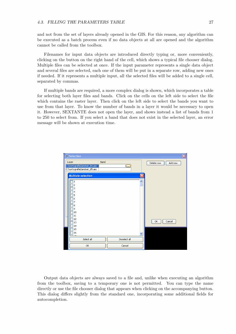
If multiple bands are required, a more complex dialog is shown, which incorporates a tablefor selecting both layer files and bands. Click on the cells on the left side to select the filewhich contains the raster layer. Then click on the left side to select the bands you want touse from that layer. To know the number of bands in a layer it would be necessary to openit. However, SEXTANTE does not open the layer, and shows instead a list of bands from 1to 250 to select from. If you select a band that does not exist in the selected layer, an errormessage will be shown at execution time.

Output data objects are always saved to a file and, unlike when executing an algorithmfrom the toolbox, saving to a temporary one is not permitted. You can type the namedirectly or use the file chooser dialog that appears when clicking on the accompanying button.This dialog differs slightly from the standard one, incorporating some additional fields forautocompletion.


If the default value (Do not autocomplete) is selected, SEXTANTE will just put the selectedfilename in the selected cell from the parameters table. If any of the other options is selected,all the cells below the selected one will be automatically filled based on a defined criteria. Thisway, it is much easier to fill the table, and the batch process can be defined with less effort.

Automatic filling can be done simply adding correlative numbers to the selected filepath,or appending the value of another field at the same row. This is particularly useful for namingoutput data object according to input ones.

Cells can be selected just clicking and dragging. Selected cells can be copied and pastedin a different place of the parameters table, making it easy to fill it with repeated values.

4.4 Setting the output region

Just like when executing a single algorithm, when running a batch process you must definethe extent of the region to be analyzed. The corresponding Output region tab is similar to theone found when running a single algorithm, but only contains two options: fit to input layersand used–defined.

The selection will be applied to all the single executions contained in the current batchprocess. If you want to use different output configurations, then you must define differentbatch processes.

4.5. EXECUTING THE BATCH PROCESS 29

4.5 Executing the batch process

To execute the batch process once you have introduced all the necessary values, just click onOK. SEXTANTE will show the progress of each executed algorithm, and at the end will showa dialog with information about the values used and the problems encountered during theexecution of the whole process.

As it happened with the iterative execution of algorithms, when executing in a batchprocess an algorithm that produces text output with numerical values (such as, for instance,statistics of a raster layer), its numerical outputs are presented in a table in the resultsmanager. Each row of the table represents an execution of the algorithm, while each columncontains the values of one of the numerical variables being calculated.

Chapter 5

The SEXTANTE command–line in-terface

5.1 Introduction

The command–line interface allows advanced users to increase their productivity and performecomplex operations that cannot be performed using any of the other elements of the SEX-TANTE GUI. Models involving several algorithms can be defined using the command–lineinterface, and additional operations such as loops and conditional sentences can be added tocreate more flexible and powerful workflows.

5.2 The interface

Invoking the command–line interface will cause the following dialog to appear.

The SEXTANTE command–line interface is based on BeanShell. BeanShell is a Javasource interpreter with object scripting language features, that meaning that it dynamicallyexecutes standard Java syntax and extends it with common scripting conveniences such asloose types, commands, and method closures like those in Perl and JavaScript.

31

32 CHAPTER 5. THE SEXTANTE COMMAND–LINE INTERFACE

A detailed description of BeanShell and its usage can be found at the BeanShell website1.Refer to it if you want to learn more about generic BeanShell features. This chapter coversonly those particular elements which are related to SEXTANTE geoalgorithms.

By using the extension mechanisms of BeanShell, SEXTANTE adds several new commandsto it, so you can run geoalgorithms or get information about the geospatial data you are using,among other things.

Java users can create small scripts and programs combining standard elements of Javawith SEXTANTE commands. However, those who are not familiar with Java can also use thecommand–line interface to execute single processes or small sets of them, simply calling thecorresponding methods.

A detailed description of all SEXTANTE commands is given next.

5.2.1 Getting information about data

Algorithms need data to run. Layers and tables are identified using the name they have inthe table of contents of the GIS (and which usually can be modified using GIS tool). To calla geoalgorithm you have to pass it an identifier which represents the data to use for an input.

The data() command prints a list of all data objects available to be used, along with theparticular name of each one (i.e. the one you have to use to refer to it). Calling it you willget something like this:

RASTER LAYERS

-----------------

mdt25.asc

VECTOR LAYERS

-----------------

Contour lines

TABLES

-----------------

Be aware that some GIS allow you two have several layers with the same name. SEX-TANTE will just take the first one which matches the specified identifier, so you should makesure you rename your data object so each one of them has a unique name.

To get more information about a particular data object, use the describe(name of data object)

command. Here are a few examples of the result you will get when using it to get more infor-mation about a vector layer, a raster layer and a table.

>describe("points")

Type: Vector layer - Point

Number of entities: 300

Table fields: | ID | X | Y | SAND | SILT | CLAY | SOILTYPE | EXTRAPOLAT |

>describe("dem25")

Type: Raster layer

X min: 262846.525725

X max: 277871.525725

Y min: 4454025.0

1www.beanshell.org

www.beanshell.org

5.3. GETTING INFORMATION ABOUT ALGORITHMS 33

Y max: 4464275.0

Cellsize X: 25.0

Cellsize Y: 0.0

Rows: 410

Cols: 601

>describe("spatialCorrelation")

Type: TableNumber of records: 156

Table fields: | Distance | I_Moran | c_Geary | Semivariance |

5.3 Getting information about algorithms

Once you know which data you have, it is time to know which algorithms are available andhow to use them.

When you execute an algorithm using the toolbox, you use a parameters window withseveral fields, each one of them corresponding to a single parameter. When you use thecommand line interface, you must know which parameters are needed, so as to pass theright values to use to the method that runs that algorithm. Of course you do not have tomemorize the requirements of all the algorithms, since SEXTANTE has a method to describean algorithm in detail. But before we see that method, let’s have a look at another one, thealgs() method. It has no parameters, and it just prints a list of all the available algorithms.Here is a little part of that list as you will see it in your command–line shell.

bsh % algs();

acccost-------------------------------: Accumulated cost(isotropic)

acccostanisotropic--------------------: Accumulated cost (anisotropic)

acccostcombined-----------------------: Accumulated cost (combined)

accflow-------------------------------: Flow accumulation

acv-----------------------------------: Anisotropic coefficient of variation

addeventtheme-------------------------: Points layer from table

aggregate-----------------------------: Aggregate

aggregationindex----------------------: Aggregation index

ahp-----------------------------------: Analytical Hierarchy Process (AHP)

aspect--------------------------------: Aspect

buffer--------------------------------: Buffer

On the right you find the name of the algorithm in the current language, which is the samename that identifies the algorithm in the toolbox. However, this name is not constant, sinceit depends on the current language, and thus cannot be used to call the algorithm. Instead,a command–line is needed. On the left side of the list you will find the command–line nameof each algorithm. This is the one you have to use to make a reference to the algorithm youwant to use.

Now, let’s see how to get a list of the parameters that an algorithms require and theoutputs that it will generate. To do it, you can use the describealg(name of the algorithm)

method. Use the command–line name of the algorithm, not the full descriptive name.

For example, if we want to calculate a flow accumulation layer from a DEM, we will needto execute the corresponding module, which, according to the list shown using the algs()

method, is identified as accflow. The following is a description of its inputs and outputs.

>describealg("accflow")


Usage: accflow(DEM[Raster Layer]

WEIGHTS[Optional Raster Layer]

METHOD[Selection]

CONVERGENCE[Numerical Value]

FLOWACC [output raster layer])

If an algorithm has a selection parameter, the value of that parameter should be enteredusing an integer value. To know the available options, you can use the options command, asshown in the following example:

In this case, the slope algorithm has two such parameters, the first one of them with 7options, and the second one with 3. Notice that ordeing is zero–based.

5.4 Running an algorithm

Now you know how to describe data and algorithms, so you have everything you need to runany algorithm. There is only one single command to execute algorithms: runalg. Its syntaxis as follows:

> runalg{name_of_the_algorithm, param1, param2, ..., paramN)

The list of parameters to add depends on the algorithm you want to run, and is exactlythe list that the describealg method gives you, in the same order as shown.

Depending on the type of parameter, values are introduced differently. The next one is aquick review of how to introduce values for each type of input parameter

• Raster Layer, Vector Layer or Table. Simply introduce the name that identifies the dataobject to use. If the input is optional and you do not want to use any data object, write“#”.

• Numerical value. Directly type the value to use or the name of a variable containingthat value.

• Selection. Type the number that identifies the desired option, as shown by the options

command

• String. Directly type the string to use or the name of a variable containing it.

• Boolean. Type whether “true” or “false” (including quotes)

• Multiple selection - data type. Type the list of objects to use, separated by commas andenclosed between quotes.

For example, for the maxvaluegrid algorithm:

Usage: runalg("maxvaluegrid",

INPUT[Multiple Input - Raster Layer]

NODATA[Boolean],

RESULT[Output raster layer])

The next line shows a valid usage example:

> runalg("maxvaluegrid", "lyr1, lyr2, lyr3", "false", "#")

5.5. ADJUSTING THE ANALYSIS REGION 35

Of course, lyr1, lyr2 and lyr3 must be valid layers already loaded into your GIS.

When the multiple input is comprised of raster bands, each element is represented by apair of values (layer, band). For example, for the cluster algorithm

Usage: runalg( "cluster",

INPUT[Multiple Input - Band],

NUMCLASS[Numerical Value],

RESULTLAYER[output raster layer],

RESULTTABLE[output table],

);

The next line shows a valid usage example:

> runalg("cluster, "lyr1, 1, lyr1, 2, lyr2, 2", 5, "#", "#")

The algorithm will use three bands, two of them from lyr1 (the first and the second onesof that layer) and one from lyr2 (its second band).

• [Table Field from XXX ]. Write the name of the field to use. This parameter is case–sensitive.

• [Fixed Table ]Tabla fija. Type the list of all table values separated by commas andenclosed between quotes. Values start on the upper row and go from left to right. Hereis an example:

runalg("kernelfilter", "mdt25.asc", "-1, -1, -1, -1, 9, -1, -1, -1, -1", "#")

• [Point ]. Write the pair of coordinates separated by commas and enclosed betweenquotes. For instance “220345, 4453616”

Input parameters such as strings or numerical values have default values. To use them,type “#” in the corresponding parameter entry instead of a value expression.

For output data objects, type the filepath to be used to save it, just as it is done from thetoolbox. If you want to save the result to a temporary file, type “#”. Use “$” to indicate thatyou want to overwrite an input layer. If the algorithm does not support overwriting, it willsave the resulting layer to a temporary file. Use “!” to indicate that an output should not becreated.

5.5 Adjusting the analysis region

If you execute from the command–line interface an algorithm that allows the user to selectthe characteristics of the analysis region, it will by default adjust it to the input layers, takingits extent (and cellsize in case of raster layers). You can toggle this behaviour using theautoextent command.

> autoextent("true"/"false)

If you want to define the analysis region manually or using a supporting layer, you haveto use the extent command, which has three different variants.


Usage: extent(raster layer[string])

extent(vector layer[string], cellsize[double])

extent(x min[double], y min[double],

x max[double], y max[double],

cell size[double])

Type "autoextent" to use automatic extent fitting when possible

When this command is used, the autoextent functionality is automatically deactivated.

5.6 Managing layers from the command–line interface

You can perform some operation with layers from the command–line interface, like the follow-ing ones:

• Opening a layer. Use the open(filepath to layer, name, view name) command.View name is the name of the view where the layer should be added, while name isthe name to give to the layer in that view.

• Closing a layer. Use the close(layer name) command.

• Changing the no–data value of a raster layer. Use the setnodata(layer name, new value)

command

• Changing the name of a layer. Use the rename(layer name, new layer name) com-mand

if you want to have the the names of layers and tables stored in a variable, so you caniterate them, you can use any of the following commands.

• getRasterLayers().

• getVectorLayers().

• getTables().

All of these commands return an array of String values with the names of the correspondingdata objects.

5.7 Creating scripts and running them from the toolbox

Scripts can be run using the source(script filename) command. Simply put your com-mands in a text file and then you can execute them calling them with a single line.

You can define new commands (methods) and save them to a file, so running that filewill load your commands and make them available for the current command-line session. Forinstance, here is an example method that calculates the slope of a DEM by all the availablemethods and then computes the mean value of all the slope layers and saves it to a temporaryfile.

slopemean(dem, meanslope){

NUMBER_OF_METHODS = 7;

multiple = "";

for(i=0;i<NUMBER_OF_METHODS;i++){

5.7. CREATING SCRIPTS AND RUNNING THEM FROM THE TOOLBOX 37

runalg("slope", dem, "#", "#", "#");

rename("Slope", "Slope" + i);

multiple = multiple + "Slope" + i;

if (i < NUMBER_OF_METHODS - 1){

multiple=multiple + ",";

}

}

runalg("multigridmeanvalue", multiple, "#", meanslope);

for(i=0;i<NUMBER_OF_METHODS;i++){

close("Slope"+i);

}

}

Assuming that this script is saved in a file named /home/myuser/slopemean.bsh, then itcould be run just entering

source("/home/myuser/slopemean.bsh");

After doing that, the slopemean command would be available and could be called with aline like the following one:

slopemean("dem", "meanslope.tif");

dem being the name of the DEM layer that we want to analyze. The file will be saved to thedefault output folder.

Scripts can be made available from the toolbox as geoalgorithms, following these rules:

• Each script must contain just one method.

• The name of the method must be the same as the name of the script file.

• The file must have the “bsh” extension.

The above example meets these three requirements.Since SEXTANTE needs some additional information to create the parameters window,

additional lines must be added to provide that information. This should be added as Javacomments before the method itself, and should have the name of the parameter(the name toshow to the user), the equal sign (=) and the type of parameter. The following keywords can beused to describe the type of a given parameter: raster, vector, table, multiple raster,

multiple vector, boolean, number, string, output raster, output vector, output

table. Comments used to define parameters should appear in the same order as they appearin the method call.

For the above example, the following comment lines should be added:

//dem=raster

//meanslope=output raster

The last step is to define the scripts folder. Only script files from that folder will be loadedas algorithms. You will find a Script tab in the setting dialog, which is very similar to theModels one that you should already know how to use.

Scripts in the scripts folder are automatically executed when the command line is opened,so their corresponding method will be available without having to call them using the source()


command. Make sure that those files contain only method definitions; otherwise, the processesthey contain will be executed as well each time you start a new command–line session (unlessyou really want that to happen...).

The SEXTANTE help folder contains several example scripts. Check them to betterunderstand how this feature works.

Chapter 6

The SEXTANTE history manager

6.1 Introduction

Every time you execute a SEXTANTE algorithm, information about the process is stored inthe SEXTANTE history manager. Along with the parameters used, the date and time of theexecution are also saved.

This way, it is easy to track the and control all the work that has been developed usingSEXTANTE, and easily reproduce it.

The SEXTANTE history manager is a set of registries grouped according to their date ofexecution, making it easier to find information about an algorithm executed at any particularmoment.

Process information is kept as a command–line expression, even if the algorithm waslaunched from the toolbox. This makes it also useful for those learning how to use thecommand–lin interface, since they can call an algorithm using the toolbox and then check thehistory manager to see how that same algorithm could be called from the command line.

Apart from browsing the entries in the registry, processes can be re–executed, simplydouble–clicking on the corresponding entry.

You can also right click on a process (the command–line sentence must start with “runalg”)and select Open algorithm dialog. This will show the dialog used to execute the algorithm,already filled with the parameter values corresponding to the selected command.

39

40 CHAPTER 6. THE SEXTANTE HISTORY MANAGER

Chapter 7

Configuring algorithm providers

7.1 Introduction

SEXTANTE can be extended using additional applications, calling them from within SEX-TANTE. This chapter will show you how to do it. Once you have configured the system,you will be able to execute GRASS and SAGA algorithms from any SEXTANTE compo-nent like the toolbox or the graphical modeler, just like you do with any other SEXTANTEgeoalgorithm.

Certain desktop GIS that incorporate SEXTANTE have both SAGA and GRASS alreadypreconfigured, so you do not have to configure any of them and their algorithms are availablein the SEXTANTE toolbox since the first time you start the program. In this case, the settingswindows contain less options then the ones described in this chapter. Using the preconfiguredsettings is always preferred, so you can skip this chapter if you are using one of those desktopGIS.

7.2 Configuring SAGA

SAGA is a GIS with a large set of geoalgorithms, most of which can be executed from SEX-TANTE. SEXTANTE will wrap SAGA algorithms and call the command–line version of SAGAusing the data entered by the user using the typical parameter panels of SEXTNATE. Beforeyou can to do so, you have to install SAGA in SEXTANTE, to let SEXTANTE know whichalgorithms are available and where to find SAGA in your computer.

To install SAGA, go to the SEXTANTE configuration dialog and select the SAGA group.You will find the next panel:

41

42 CHAPTER 7. CONFIGURING ALGORITHM PROVIDERS

Just enter the path to the folder where the SAGA executables are located and then pressthe Install SAGA button. SEXTANTE will tell SAGA to describe its algorithms and, basedon these descriptions, will generate the corresponding SEXTANTE algorithms.

A message dialog will appear, showing the number of algorithms that have been found.When you close the settings dialog, the toolbox will be updated and it will contain a newgroup named SAGA.

If you do not want SAGA algorithms to be shown in the toolbox, just uncheck the Activatecheckbox. To activate it back you do not need to reinstall SAGA, since the text files thatdescribe SAGA algorithms are already created in your system. Just check the checkbox andclose the settings dialog.

7.3 Configuring GRASS

GRASS GIS is a very powerful system that can process large amounts of 2D and 3D, rasterand vector data with ease. It was designed as a collection of tools (modules) that can be runfrom the command line individually. The SEXTANTE–GRASS interface aims to bring thelargest part of that rich functionality to SEXTANTE users.

This section describes how to configure SEXTANTE so it can call GRASS algorithms andincorporate them into its own set of geoalgorithms. It also gives some additional informationon the mechanism used by SEXTANTE to integrate GRASS modules, which should be usefulfor all users, but specially for those familiar with the GRASS command-line interface.

Open the settings dialog and select the GRASS menu page. The following parametersmust be set:

• The path to the folder into which GRASS was installed on your system. Needed by SEX-TANTE to execute GRASS commands. Under Linux, this is frequently usr/lib/grassXX(for GRASS installed with a package manager) or /usr/local/grassXX (if compiled andinstalled from source code).

• The path to a GRASS mapset. The mapset doesn’t have to contain any data at all,since data will be imported automatically each time you execute an algorithm. The

7.3. CONFIGURING GRASS 43

GRASS interface is totally ignorant of projection setttings. When data is processed,no reprojection is performed, and layers are assumed to be in the same projection asthe mapset itself. So make sure that youonly process data with matching spatial refer-ence systems. Otherwise, accurate results cannot be guaranteed. If you do not have aGRASS mapset, you can ask SEXTANTE to create a temporary one for you. Select thecorresponding checkbox and a new one will appear instead of the texbox for selectingthe mapset folder. In order to create the temporary mapset, SEXTANTE needs to knowwhether your data will use geographic coordinates (lat/lon) or projected ones. Checkthe new box accordingly. The temporary mapset and all data in it will automaticallybe deleted when the processing is done.

• The path to a shell interpreter. Only if you are running Windows, you need to specifya shell interpreter (Linux and Mac OS X include one as part of the system). A fullyfunctional shell interpreter, including the most important tools, is provided by the MSYS(Minimal SYStem) open source project. Some GRASS modules are shell scripts thatneed additional command line tools. If they are not all found then a warning willbe issued. Check the SEXTANTE History’s Warnings page to see which commandsmay be missing from your system. Some distributions of GRASS for Windows a shellenvironment, usually installed in [GRASS folder]/msys/bin, but you can use one in adifferent location. Select the corresponding path in the textbox (you need to locate theexecutable sh.exe).

If you wish to process 3D vector data with GRASS, then you must activate the corre-sponding setting (3D input data will not automatically be recognized as such). You may alsochoose to import polygons as polylines instead.

Once you have set the above paths, click on Setup GRASS to finish configuring theSEXTANTE–GRASS interface. SEXTANTE will now try to execute GRASS and createthe definition files that are used to generate the graphical interfaces of all the suitable GRASSalgorithms, along with the corresponding help files. This process might take a few seconds. Ifeverything goes well, you can close the settings dialog by clicking on the OK button. GRASSalgorithms will now be shown in the toolbox and identified with a GRASS icon. They willappear in a new branch named GRASS in the algorithms tree, which contains two groups:raster (r.*) and vector (v.*), and also in the usual groups used for built–in SEXTANTE al-gorithms. This way, it is easier to find the right algorithm, both for SEXTANTE users withno previous GRASS experience and former GRASS users.

Not all GRASS algorithms are available from SEXTANTE. Some of them are not compat-ible with the architecture of SEXTANTE and its algorithm-definition semantics, while othersdo not make much sense in the context of SEXTANTE (like, for instance, those used to digitizeand create new vector layers). Unsuitable algorithms are automatically removed and will notappear in any SEXTANTE component.

7.3.1 Usage notes and limitations

GRASS is a system that consists of hundreds of independent, loosely coupled, programs de-signed to be run from the command line. There are some complexities in trying to wrap agraphical user interface (GUI) around such an architecture. It can never be done perfectly,but the GRASS–SEXTANTE interface goes to some lengths in order to ensure a smooth userexperience.

There are several different versions of GRASS available. Currently, the GRASS-SEXTANTEinterface has been tested and designed to run with GRASS 6.4. Other GRASS versions mayor may not work.


If you notice anything wrong with a particular GRASS module, please post a message tothe SEXTANTE users mailing list, notifying us of your concern. We will try to fix it for thenext release.

The current version of the SEXTANTE-GRASS interface offers good support for most ofthe GRASS raster and vector processing modules. Most significantly, it does not support theimagery (i.*) and voxel (3D raster; r3.*) processing modules. Users who want access to thefull power and flexibility of GRASS GIS are advised to install GRASS on an operating systemwith good POSIX compatibility (such as Linux or Mac OS X) and learn to use it from thecommand line.

Message output from GRASS modules

Many GRASS modules produce verbose and important output as part of their processing.This can be reviewed after a GRASS module has run, by opening the GRASS output pageof the SEXTANTE History. This is always a good idea, especially when unexpected resultsoccur.

Some modules do not output error messages in a standard way, so that errors can bedetected and a message displayed by SEXTANTE. If a module produces an empty or noresult, check the full GRASS messages transcript in the SEXTANT log browser.

Graphical interface

Those GRASS modules that can produce a multitude of optional outputs will be split up into”sibling” algorithm, one for each optional output. Siblings share the same name with the”parent” algorithm (the one with the full set of parameters) but have an additional specifierin ”()”.

Sometimes, a certain option is impossible or pointless to replicate in the GUI and willthus be skipped, leading to discrepancies with the official GRASS module documentation. Aprime example is the ”layer=” option which many GRASS vector modules employ to let theuser switch between different attribute tables connected to the same ”layer” (which is actuallycalled a ”map” in GRASS lingo).

Some modules upload data into existing or new attribute tables for an existing input vectordataset. Such modification will be lost after the GRASS command finishes. We have tried toencapsulate the most important ones using a postprocessing function which will export thenew attribute table fields together with a copy of the original input dataset as a new vectorlayer. In this way, modules such as v.distance become fully functional. However, this is not auniversal solutions and some modules that modify the attribute table structure of an existinginput vector dataset are still likely to lose these changes.

Vector data exchange

The GRASS interface currently uses ESRI Shapefiles as a kind of lowest common denominatorto exchange data between SEXTANTE and GRASS. Shapefiles have severe limitations, whichmay also be felt when processing vector data with the SEXTANTE–GRASS interface. Theselimitations do not exist in the native GRASS vector models but are caused by having to relyon the much simpler Shapefiles for data exchange.

The most obvious limitation is the fact that Shapefiles can only store one type of geometricprimitive each (point, line or polygon). The output of GRASS modules that produce multi–type geometries will automatically split into separate files for the primitives.

In addition, since Shapefiles use DBase files for attribute data, all limitations associatedwith that file format also apply.


Output vector maps will have a “cat” column or (if that already exists) a “ cat” column,which are the internal primary keys used by GRASS to link vector objects with attibute tablefields. Apart from being a waste of bytes in the output file, GRASS modules will fail to runon input vector maps that already have both “cat” and “ cat” field. So it is a good idea todelete them manually from the attribute table. Unfortunately, the current official version ofGRASS does not yet offer a safe way of doing this automatically.

(Please also make sure to read the notes on topology below)

Raster data exchange

There are no severe limitations for raster data processing via the SEXTANTE–GRASS inter-face.

However, there is no simple support for setting the GRASS raster MASK yet. If youneed one, then you must create a GRASS mapset externally and then create a mask in there.Then use SEXTANTE to connect to that mapset. They mask will now be active for all rasteroperations carried out through the SEXTANTE GRASS interface.

Topology

GRASS is one of the few GIS that insist on keeping a strict topological model for all vectordata that goes through it. This ensures reliable operation and correct output, but means thattopologically unclean data may be a challenge to process without first cleaning it (”garbagein, garbage out”).

One common source of problems are overlapping polygons in one input file. The latter arenot allowed in the 2D topology model that GRASS uses. GRASS will employ an automatedcleaning process on such data which will most likely result in some of the polygons beingdiscarded.

Note that the GRASS vector model currently has no valid topological representation forarbitrary 3D polygons (as opposed to simple 3D triangles, so called ”faces”, which make upmeshes such as TINs). Getting such data past the (unfortunately) 2D topological cleaningmechanism of GRASS without having it ”butchered” can be a challenge. In those cases whereonly the geometry information (not the attribute data) is of interest, setting the GRASSinterface options to import polygons as polylines may provide a solution.

The GRASS region

GRASS GIS offers many ways of setting the computation region’s extent and resolution on-the-fly. Doing this is only mandatory for modules with raster output (except raster importmodules: r.in.*). But may also be important for some others (such as v.voronoi), whose resultdepends on the extent of the region, nonetheless. So the region settings are always availableon the Region tab of each GRASS module’s GUI.

7.3.2 Windows notes

Due to its design, GRASS does not run as smoothly on Windows as it does on other operatingsystems, since the latter lacks some POSIX features for inter–process communication. Forthe user, the most significant effect of this is that SEXTANTE cannot display an accurateprogress bar for GRASS commands running on Windows.

There is also no support for mapset locking on the Windows platform. So the user musttake care not to use a mapset for processing which might be in use by another person at thesame time.


7.3.3 Notes on specific modules

These are some usage hints for some interesting GRASS modules, which may not be obviousto GRASS novices. They also serve to illustrate common principles of GRASS usage via theSEXTANTE-GRASS interface.

r.colors(.stddev)

GRASS provides some beautiful, automatically adjusted color schemes for raster data. Youcan use “r.colors” to pick a scheme, but the new color scheme can only be applied to the resultif the GIS that you run SEXTANTE under can handle external color map definitions in theformat which the SEXTANTE-GRASS interface uses. At the moment, this is only true forgvSIG.

Note also that the result will be returned as a new layer, as the SEXTANTE–GRASSinterface cannot directly manipulate the input layer.

r.in/out.gdal

Raster data in a variety of formats can be imported and exporting using r.in.gdal and r.out.gdal,respectively. These modules use the geodata drivers provided by the GDAL project1. See theproject’s web page for details about the level of support for the different formats.

r.mapcalculator

This is a GRASS script that wraps the powerful r.mapcalc tool, which is a commandline–onlytool for raster map algebra in GRASS. If you want to get an idea of all its capabilities, findthe HTML manual page for r.mapcalc in your local GRASS installation or on the web.

How to use r.mapcalculator: Specify up to six input layers to be used and then referencethem in the “formula=” field. You can A,B,C etc . or amap,bmap,cmap etc. Don’t worryabout putting in quotation marks (“). That will be done automatically. Here is an exampleof an expression that shows how to use the null() function and the if() conditional function:“if(A=¿500,A,null())”. This will filter out all cells of a DEM (input as map A) that lie below500 m.

r.null

You can very easily set a (range of) cell value(s) to “no data” (NULL) usig this module. Notethat the result will be returned as a new layer, as the SEXTANTE–GRASS interface cannotdirectly manipulate the input layer.

v.in/out.ogr

You can import and export several vector data formats using the v.in.ogr and v.out.ogr com-mands. The OGR drivers cater for a number of different vector data sources, so the interfacesemantics have been built around “dsn=” (data source) and “layer=” (layer within a datasource) specifiers. The SEXTANTE–GRASS interface will allow you to simply select a fileusing the file selector behind the “dsn=” parameter.

For exporting data with v.out.ogr, make sure to select the right data format. If you skipthe extension, the right one will automatically be added to the output file. For most formats,you can simply enter a path and file name into the “olayer” option field. Please consult the

1http://www.gdal.org

http://www.gdal.org


GDAL/OGR documentation for individual format details (e.g. set the “lsco” option value to“format=mif” if you want to create MapInfo ASCII vector output).

OGR is a subproject of GDAL, so details about the different formats can be found on thesame project page. As with GDAL, the drivers supported will depend on your local versionof the GDAL library.

Note that due to the use of Shapefiles for data exchange, multiple-geometry-type formats(such as MapInfo) are supported, but they will be split into single-geometry files after import.

v.surf.bspline

GRASS has some very flexible modules for spline curves based interpolation. The tricky partof v.surf.bspline is that you have to set the “layer” option to 0 if you want to interpolate thethe Z coordinates of the input points directly. If you want to interpolate based on an attributetable field, set “layer=1” and then enter the name of the field as “column”.

v.surf.idw

This is a very capable, but also complex spline-based interpolation module. Getting high-quality output requires some knowledge about the many different parameters. Note that, dueto the SEXTANTE interface semantics, at least on raster layer must be present in your projectbefore the module becomes available.

v.to.3d

This module offers a convenient way to cast 2D vector data to 3D (or the other way around).The interface was tweaked a litte so that it can run under SEXTANTE. Enter a constant heightvalue into “height”, or leave height at the default setting and additionally enter an attributefield name into “column”. But “height” must always be set (at least to some dummy value).

Make sure to check the 3D data processing setting in the GRASS settings!

7.3.4 Technical details

If you are a GRASS user, it might be useful for you to know how SEXTANTE calls GRASS al-gorithms and comunicates with the GRASS interface. This can be summarized in the followingsteps:

• Importing data. The layers that have been selected as input are imported into the(temporary or existing) GRASS mapset. Not every layer that you can open in yourGIS can be used to execute a GRASS algorithm. It must be a file-based layer and itmust have a format compatible with the capabilities of the GRASS modules that importexternal data. Refer to the GRASS help files for further information.

• Processing. The selected GRASS algorithm is executed.

• Exporting results. Resulting data are exported to the filenames selected by the user inthe input parameters dialog. Only layers (whether raster or vector) are exported. Also,take into account that exporting data also has its limitations, and not all the informationgenerated might be available. For instance, topological information will be lost, sincedata are exported to Shapefile format, which cannot store it. for further details, checkthe help file associated with GRASS export modules.


All this steps are stored in a batch file that is executed using the GRASS BATCH JOBvariable. When SEXTANTE invokes GRASS, the commands in the batch file are executedand GRASS closes up automatically after that.

Introduction to SEXTANTE (v0.7)gvsigce.sourceforge.net/.../IntroductionToSEXTANTE.pdf ·...

Documents

Transcript of Introduction to SEXTANTE (v0.7)gvsigce.sourceforge.net/.../IntroductionToSEXTANTE.pdf ·...