Introduction to R for Social Scientists∗

Elizabeth Menninga†

Odum Institute for Research in Social ScienceUniversity of North Carolina at Chapel Hill

January 24–25, 2013

1 Course Overview• Day 1

Getting started

Basics of objects, functions, etc. . .

Probability

Loading and working with data

• Day 2

Introduction to graphics

Basic programming

Numerical optimization

Advanced graphics

Questions/other topics

2 What is R?R is a platform for the object-oriented statistical programming language S. It is widely used in statistics

and has become quite popular in the social sciences over the last decade. Essentially R can be used as eithera matrix-based programming language or as a standard statistical package that operates much like Stata,SAS, or SPSS. It also carries an extensive library of user-written packages that can be used to conduct awide variety of statistical analyses, graphical presentations, and other functions.

2.1 Where can I get R?The beauty of R is that it is free to anyone. To obtain R for Windows, Mac, or Linux go to The Com-

prehensive R Archive Network (CRAN) at http://www.r-project.org/. Just download the executablefile, and it will install itself.1 Unfortunately, there are no update patches, so you must completely install anew version whenever you would like to upgrade.∗These notes draw from short courses taught by Luke Keele, Evan Parker-Stephen, Jamie Monogan, and Jeff Harden.†Department of Political Science, University of North Carolina at Chapel Hill, menninga[at]email.unc.edu1Linux users will find it easier to install from a terminal. Terminal code is available at http://monogan.myweb.uga.

edu/computing/linux/index.htm.

1

2.2 Using R with a Text EditorR is an actual programming language. This means you type code and submit it rather than the point-

and-click approach. Code is usually saved in “script files” with the “.R” file extension. I strongly rec-ommend using a text editor such as Tinn-R (for Windows users) or RStudio (for both Windows and Macusers) to manage script files. This makes submitting commands to R quicker, organizing your code eas-ier, and protects you from losing code if R crashes. Other options exist besides RStudio and TinnR, sofeel free to explore if you don’t like the functionality of these. Other text editors can be found here:http://www.sciviews.org/_rgui/projects/Editors.html.

RStudio (and most of the other available text editors) has lots of features that are useful, such as its“replace” feature. By typing Ctrl + R, you can replace text in the code with new text. This is very helpfulif you have a string of text that is repeated several times in the code and needs to be changed. It alsocolor codes different types of commands, which can help you identify errors more easily, potentially evenpreemptively.

2.3 Installing RStudio• Download RStudio here: http://www.rstudio.com/.

• Open RStudio and begin working!

2.4 Installing Tinn-R• Download Tinn-R here: http://www.sciviews.org/Tinn-R/.

• Once Tinn-R is loaded, open Tinn-R and R.

• In Tinn-R, select R→ Start/close and connections→ Rgui (start).

• If you would like to arrange the two windows vertically, go to Options → Application → R →Rgui→ Options.

2.5 ResourcesAs questions emerge when you use R, here are a few resources you may want to consider:

• Within R, there is “Introduction to R,” which is under the “Help” pull down menu under “Manuals”,as well as the ?, ?? and help() commands.

• To do a web-based search, use http://www.rseek.org/ (powered by Google).

• Odum resources on the website: http://www.odum.unc.edu/odum/contentSubpage.jsp?nodeid=670.

• Quick-R is a great resource for SAS/SPSS/Stata users: http://www.statmethods.net/.

• There are many good books on R, including Fox (2002), Verzani (2005), Braun and Murdoch (2007),and Cohen and Cohen (2008).

• Springer publishes several books from the Use R! series: http://link.springer.com/bookseries/6991.

2

3 First Steps

3.1 Entering commandsOnce you have R open, you can start right away. All of the commands you will use will be entered

through the command line:

>

3.2 Object-oriented programming (OOP)From WIKIPEDIA:

A programming paradigm that uses “objects”—data structures consisting of datafields andmethods together with their interactions—to design applications and computer programs. Pro-gramming techniques may include features such as information hiding, data abstraction, en-capsulation, modularity, polymorphism, and inheritance.

As complicated as this sounds, OOP makes R easy and flexible! In non-programming-speak, it meansthat you can store anything you do in R as an object with a name, then look at that object, run anothercommand on it later, overwrite it, or delete it as you see fit. Here is a basic example. I want to create anobject called x that is the value 2. I use the assignment operator, which is the less-than sign and a hyphen,(<-) to do this:

x <- 2

x

[1] 2

You can use R as a calculator. Storing various objects and calculations as you go for future use.

y<-log(10) #note: log() is log base e. log10() is log base 10

x+y

[1] 4.302585

a<-x+y^2 # R follows order of operations (PEMDAS) but still be careful

a

[1] 7.301898

3.3 Some tips on objects• Expressions and commands in R are case-sensitive.

• Anything following the pound character (#) R ignores as a comment. Take advantage of this toannotate your code!

• An object name must start with an alphabetical character, but may contain numeric characters there-after. A period may also form part of the name of an object. For example, x.1 is a valid name foran object in R.

• Object names cannot have spaces.

3

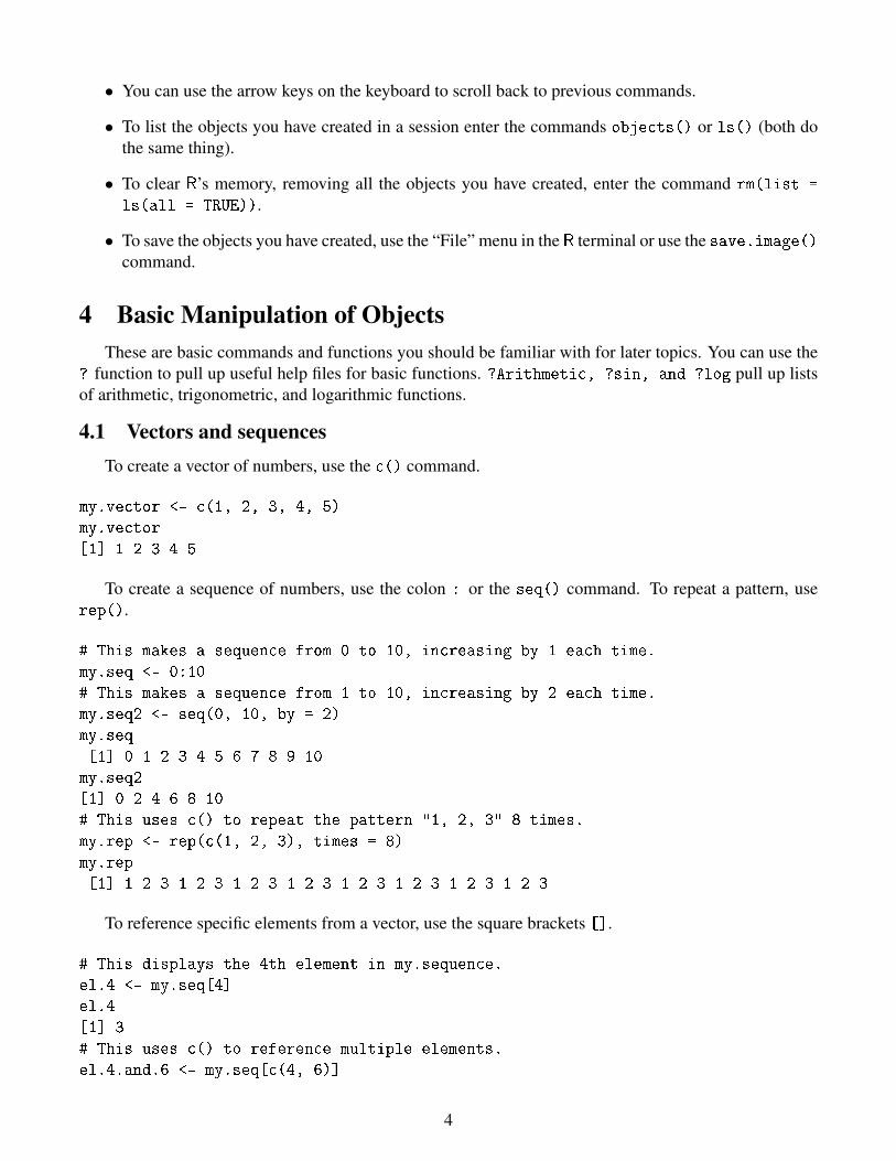
• You can use the arrow keys on the keyboard to scroll back to previous commands.

• To list the objects you have created in a session enter the commands objects() or ls() (both dothe same thing).

• To clear R’s memory, removing all the objects you have created, enter the command rm(list =

ls(all = TRUE)).

• To save the objects you have created, use the “File” menu in the R terminal or use the save.image()command.

4 Basic Manipulation of ObjectsThese are basic commands and functions you should be familiar with for later topics. You can use the

? function to pull up useful help files for basic functions. ?Arithmetic, ?sin, and ?log pull up listsof arithmetic, trigonometric, and logarithmic functions.

4.1 Vectors and sequencesTo create a vector of numbers, use the c() command.

my.vector <- c(1, 2, 3, 4, 5)

my.vector

[1] 1 2 3 4 5

To create a sequence of numbers, use the colon : or the seq() command. To repeat a pattern, userep().

# This makes a sequence from 0 to 10, increasing by 1 each time.

my.seq <- 0:10

# This makes a sequence from 1 to 10, increasing by 2 each time.

my.seq2 <- seq(0, 10, by = 2)

my.seq

[1] 0 1 2 3 4 5 6 7 8 9 10

my.seq2

[1] 0 2 4 6 8 10

# This uses c() to repeat the pattern "1, 2, 3" 8 times.

my.rep <- rep(c(1, 2, 3), times = 8)

my.rep

[1] 1 2 3 1 2 3 1 2 3 1 2 3 1 2 3 1 2 3 1 2 3 1 2 3

To reference specific elements from a vector, use the square brackets [].

# This displays the 4th element in my.sequence.

el.4 <- my.seq[4]

el.4

[1] 3

# This uses c() to reference multiple elements.

el.4.and.6 <- my.seq[c(4, 6)]

4

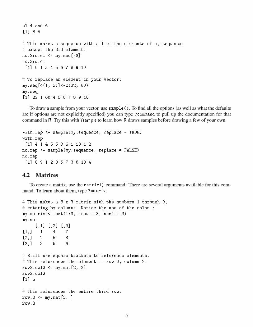
el.4.and.6

[1] 3 5

# This makes a sequence with all of the elements of my.sequence

# except the 3rd element.

no.3rd.el <- my.seq[-3]

no.3rd.el

[1] 0 1 3 4 5 6 7 8 9 10

# To replace an element in your vector:

my.seq[c(1, 3)]<-c(22, 60)

my.seq

[1] 22 1 60 4 5 6 7 8 9 10

To draw a sample from your vector, use sample(). To find all the options (as well as what the defaultsare if options are not explicitly specified) you can type ?command to pull up the documentation for thatcommand in R. Try this with ?sample to learn how R draws samples before drawing a few of your own.

with.rep <- sample(my.sequence, replace = TRUE)

with.rep

[1] 4 1 4 5 5 8 6 1 10 1 2

no.rep <- sample(my.sequence, replace = FALSE)

no.rep

[1] 8 9 1 2 0 5 7 3 6 10 4

4.2 MatricesTo create a matrix, use the matrix() command. There are several arguments available for this com-

mand. To learn about them, type ?matrix.

# This makes a 3 x 3 matrix with the numbers 1 through 9,

# entering by columns. Notice the use of the colon :

my.matrix <- mat(1:9, nrow = 3, ncol = 3)

my.mat

[,1] [,2] [,3]

[1,] 1 4 7

[2,] 2 5 8

[3,] 3 6 9

# Still use square brackets to reference elements.

# This references the element in row 2, column 2.

row2.col2 <- my.mat[2, 2]

row2.col2

[1] 5

# This references the entire third row.

row.3 <- my.mat[3, ]

row.3

5

[1] 3 6 9

#To make a matrix from previously defined vectors use rbind() or cbind()

v1<-c(1, 2, 3, 4, 5)

v2<-c(0, 1, 0, 1, 0)

v3<-c(.1, .2, .7, .4, .1)

data.mat<-cbind(v1, v2, v3)

data.mat

v1 v2 v3

[1,] 1 0 0.1

[2,] 2 1 0.2

[3,] 3 0 0.7

[4,] 4 1 0.4

[5,] 5 0 0.1

5 FunctionsR is built on lots of different functions. Here are a few more.

# Calculate the minimum, maximum, mean, median,

# and 25th and 75th percentiles of my.sequence.

min(my.seq)

[1] 0

max(my.seq)

[1] 10

mean(my.seq)

[1] 5

median(my.seq)

[1] 5

quantile(my.seq, .25)

25%

2.5

quantile(my.seq, .75)

75%

7.5

# Or we could just use the summary() function

summary(my.seq)

Min. 1st Qu. Median Mean 3rd Qu. Max.

0.0 2.5 5.0 5.0 7.5 10.0

# Two more: variance and standard deviation

var(my.seq)

[1] 11

sd(my.seq)

[1] 3.316625

#Correlation between 2 variables

cor(v2, v3)

[1] 5.963825e-17

6

#Dimensions of the vector/matrix

length(v1)

[1] 5

dim(data.mat)

[1] 5 3

5.1 Matrix algebra functionsR can also perform several useful matrix calculations and perform linear algebra:

• det(): determinant of the matrix.

• diag(): references main diagonal of the matrix.

• t(): transpose of the matrix.

• solve(): inverse of the matrix.

• eigen(): eigenvalues/eigenvectors of the matrix.

• Matrix multiplication is done by putting the % sign on either side of the *: A %*% B.

You can nest these functions together to perform more complicated tasks. Let’s pretend that we wantedto calculate the coefficients for the effect of v1, v2, and v3 on some dependent variable (and for somereason have to use old-school matrix algebra to do so). Pretend this DV of interest is DV<-c(9, 8, 7, 6,5). Then we could generate a data matrix (let’s call it data.mat2) and use matrix algebra to solve for thecoefficients.

DV<-c(9, 8, 7, 6, 5)

data.mat2<-cbind(1, v1, v2, v3)

solve(t(data.mat2) %*%data.mat2)%*%t(data.mat2)%*%(DV)

[,1]

1.000000e+01

v1 -1.000000e+00

v2 -2.220446e-15

v3 -3.552714e-15

5.2 Creating functionsR also has a function that let’s you make your own function. It is called function(). In its simplest

form, you list the arguments your new function will take, define the calculations the function will do, andfinally tell it what to return when it is done. For example, let’s make a function called average() that willcalculate the mean of a vector.

# This function requires one argument, a vector, called "the.vector" here

average <- function(the.vector){ # Start the function.

S <- sum(the.vector) # Step one: Take the sum of all elements in the.vector.

L <- length(the.vector) # Step two: Find no. of elements in the.vector.

7

A <- S/L # Divide to get the average.

return(A) # Only return the final result.

} # Close the function.

# Check to make sure it works.

average(my.seq)

mean(my.seq)

This is a very simple function that already exists in R, but the true strength of R over other stats softwareis that you can write a function that will do just about anything you desire. So if what you want doesn’talready exist, you can write a function to make it exist.

6 Probability Distributions and Random Number Generation

6.1 Basic commandsR allows you to use a wide variety of distributions for four purposes: the cumulative distribution func-

tion (cdf), probability density function (pdf), quantile function, and random draws from the distribution.All probability distribution commands consist of a prefix and a suffix. Table 1 presents the four prefixes,and their usage, as well as the suffixes for some commonly-used probability distributions.

Table 1: Probability Distributions in R

Prefix Usage Suffix Distribution

p cumulative distribution function norm normald probability density function logis logisticq quantile function t tr random draw from distribution f F

unif uniformpois poissonexp exponentialchisq χ2

binom binomial

Here are some examples with the normal distribution.

# Use the cdf to calculate the probability a random draw will be less than a given number.

pnorm(1.645)

[1] 0.950015

dnorm(1.5) # Use the pdf to calculate density.

[1] 0.1295176

qnorm(.95) # Use the quantile function to calculate quantiles from p-values.

[1] 1.644854

rnorm(10) # Random draws

[1] -0.69773442 -1.23958980 0.45287840 0.42454633 -1.51173885

[6] -0.13426599 -0.15625090 -1.01570950 -0.07550530 0.04255699

8

#Try nesting some commands we've learned

matr<-matrix(rnorm(100, mean=10, sd=2), nrow=10, ncol=10)

Let’s write a function to calculate the p-value (2-tailed) given a known t-statistic and degrees of free-dom.

p.value<-function(t.stat, df){

abs(t.stat)

2*(1-pt(t.stat, df))

}

#Test it out with t.stat=-2.4, deg.free=1,000

p.value(-2.4, 1000)

[1] 0.01657708

#Check our function

2*pt(-2.4, 1000)

[1] 0.01657708

We haven’t learned how to make graphs yet, but here are some examples with the binomial distribution.

#Binomial example

trials <- 50 # 50 trials

x <- seq(0, trials, by = 1)

y <- dbinom(x, trials, .2) # n = 50, p = .2.

plot(x, y)

y <- dbinom(x, trials, .6) # n = 50, p = .6.

plot(x, y)

z <- rbinom(100, trials, .2) # Draw 100 values from a binomial with n = 50, p = .2.

plot(density(z)) # Plot the density of those draws.

6.2 Setting the seedYou will likely use the random draw commands the most. These commands work well for nearly all

applications, but it should be pointed out that they only mimic random processes. The engine drivingthose commands is a complicated algorithm called a random number generator (RNG). Several of thesealgorithms—which have cool names like “Mersenne-Twister”, “Super-Duper”, and “white noise”—areavailable in R (see ?RNG). The most important thing for most of us is that because these algorithms aredeterministic processes, we can control the numbers they produce by setting the starting value (the “seed”).I recommend using the set.seed() command at the top of any script file in which you use a RNG. Thismight be a Monte Carlo simulation or code to draw a predicted probability plot—both topics we will getto later. You can pick any number, though usually large numbers are recommended.

For example, say you saved the following two lines in a script file:

set.seed(123456)

k <- rnorm(100)

If you opened R, entered these lines, then closed R, opened it again, and entered these lines again, youwould get the same “random numbers.” Note that you won’t get the same numbers if you just repeat the

9

lines in the same session. That is because the RNG algorithms are designed to go for very long sequencesbefore they repeat. Setting the seed just means the same numbers will appear if you start a new R session.This is very important for replication purposes. If you publish an analysis, you want someone to be ableto reproduce your exact results.

Let’s all try again it and see if we get the same numbers

set.seed(123456)

rchisq(10, 2) #take a random draw of 10 numbers with df=2

[1] 2.5266323 0.6477107 0.1605546 6.7214985 2.5282667 3.7172530 7.6708921

[8] 3.3345119 0.4881194 5.3888810

7 Working with DataR has full capabilities to clean, manipulate, and analyze data. However, I think data-cleaning is a

weakness of R and so I prefer to clean data in Stata or Excel, then load it into R for analysis. We’ll learn acouple tricks along the way, but for a more thorough discussion of the data-cleaning capabilities of R, seehttp://www.statmethods.net/management/index.html.

In short, R treats the data like a matrix. You can use any and all matrix commands to modify, change,and organize the data. This includes cbind(), rbind(), and t().

7.1 Loading dataR can read data from several formats, such as CSV files (type the command ?read.csv), R generated

tables (type ?read.table) or from several different software packages. We will use this last approach today.The first thing to do is to load our first user-written package:

install.packages("foreign") # This step is not necessary after the first time.

library(foreign)

We will use data that is based upon from Hogan (2008), an article on the effects of partisan voting byincumbents in state legislatures on their re-election chances.2 Locate the file “hogan.dta” and load it intoR with the following command:

# Change the file path appropriately, using forward slashes (/).

hogan <- read.dta("hogan.dta")

#Or to open a browser to search for the file

hogan<-read.dta(file.choose())

Once this is loaded, you can inspect the data. To look at the data in any R editor, type fix(hogan).To look at just the variable names, use the names() command.

names(hogan)

[1] "year" "chamber" "politica" "majorpar"

[5] "twoparty" "pastgene" "chamberc" "populati"

[9] "legislat" "partyadv" "incumben" "legisl_a"

2Note: I did not collect these data, so they are only for class use. Also, I have changed some of the variables from theoriginal data set to fit our needs, so the toy dataset you have is not that used by Hogan in his publication.

10

[13] "partisan" "incumb_a" "challeng" "interact"

[17] "intera_a" "challe_a" "state" "res"

[21] "challenged"

To determine if there is missing data, use the unique() and is.na() commands. In this case, novariables have missing data. If there were missing values, we could use the na.omit() command.

unique(is.na(hogan))

year chamber politica majorpar twoparty pastgene chamberc

1 FALSE FALSE FALSE FALSE FALSE FALSE FALSE

populati legislat partyadv incumben legisl_a partisan incumb_a

1 FALSE FALSE FALSE FALSE FALSE FALSE FALSE

challeng interact intera_a challe_a state res challenged

1 FALSE FALSE FALSE FALSE FALSE FALSE FALSE

When R reads a data set, it becomes a data frame. To reference specific variables in the data frame,use dollar sign ($). For example, to summarize the variable partisan, type

summary(hogan$partisan)

Min. 1st Qu. Median Mean 3rd Qu. Max.

-12.3700 0.3322 0.7136 0.6501 1.1450 10.4200

The apply command is often the most efficient way to do calculations like this. For example, tocalculate the means for all the variables in the hogan data set us you could quickly type the following. Inthis case, the argument 2 signifies we want to do this to columns. Use 1 for rows. Also, notice I deletedthe 19th column because that is not a numeric variable.

apply(hogan[-19], 2, mean) #The 2 says apply this to the columns.

year chambe politica majorpar twoparty

0.463105727 0.181718062 0.446035242 0.575991189 62.927141431

pastgene chamberc populati legislat partyadv

65.764317181 42.720087966 70.161775425 0.229822133 3.922356819

incumben legisl_a partisan incumb_a challeng

1.000000000 0.312224670 0.650061340 -0.077669530 -0.666682149

interact intera_a challe_a res challenged

-0.050102812 -0.390434266 53.738247213 0.000000061 0.763766520

7.2 Logical statementsLogical statements in R are evaluated as to whether they are TRUE or FALSE. Table 2 summarizes the

different logical operators in R.For example, how many incumbents spent more money than average in 1998? The answer: 441.

# This evaluates to TRUE or FALSE

high.spend.1998 <- hogan$incumb_a >= mean(hogan$incumb_a) & hogan$year == 1

# This makes a table out of high.spend.1998

table(high.spend.1998)

high.spend.1998

FALSE TRUE

1375 441

11

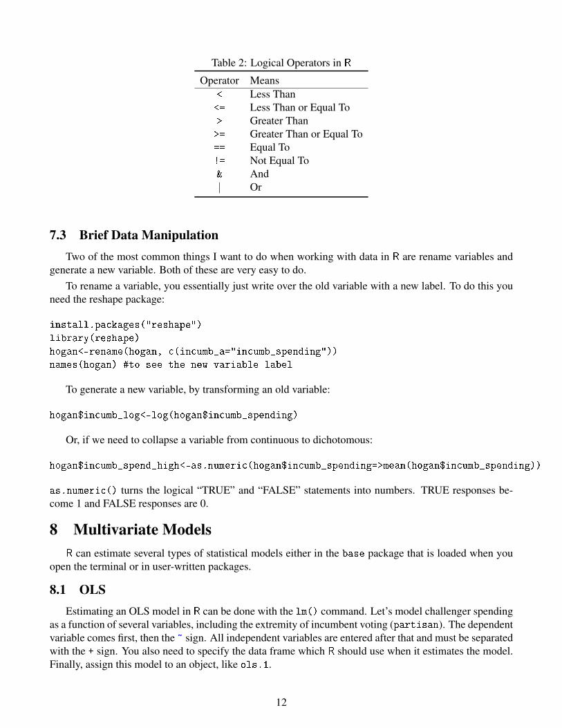
Table 2: Logical Operators in R

Operator Means< Less Than<= Less Than or Equal To> Greater Than>= Greater Than or Equal To== Equal To!= Not Equal To& And| Or

7.3 Brief Data ManipulationTwo of the most common things I want to do when working with data in R are rename variables and

generate a new variable. Both of these are very easy to do.To rename a variable, you essentially just write over the old variable with a new label. To do this you

need the reshape package:

install.packages("reshape")

library(reshape)

hogan<-rename(hogan, c(incumb_a="incumb_spending"))

names(hogan) #to see the new variable label

To generate a new variable, by transforming an old variable:

hogan$incumb_log<-log(hogan$incumb_spending)

Or, if we need to collapse a variable from continuous to dichotomous:

hogan$incumb_spend_high<-as.numeric(hogan$incumb_spending=>mean(hogan$incumb_spending))

as.numeric() turns the logical “TRUE” and “FALSE” statements into numbers. TRUE responses be-come 1 and FALSE responses are 0.

8 Multivariate ModelsR can estimate several types of statistical models either in the base package that is loaded when you

open the terminal or in user-written packages.

8.1 OLSEstimating an OLS model in R can be done with the lm() command. Let’s model challenger spending

as a function of several variables, including the extremity of incumbent voting (partisan). The dependentvariable comes first, then the ~ sign. All independent variables are entered after that and must be separatedwith the + sign. You also need to specify the data frame which R should use when it estimates the model.Finally, assign this model to an object, like ols.1.

12

ols.1 <- lm(challe_a ~ partisan + politica + majorpar + legisl_a +

partyadv, data = hogan)

To see the output type

summary(ols.1)

Call:

lm(formula = challe_a ~ partisan + politica + majorpar + legisl_a +

partyadv, data = hogan)

Residuals:

Min 1Q Median 3Q Max

-77.34 -41.49 -15.53 26.14 606.41

Coefficients:

Estimate Std. Error t value Pr(>|t|)

(Intercept) 58.6408 2.8767 20.385 < 2e-16 ***

partisan 4.2209 1.2667 3.332 0.000879 ***

politica -3.0916 2.9389 -1.052 0.292964

majorpar 3.5599 3.2474 1.096 0.273118

legisl_a -22.0720 3.1913 -6.916 6.4e-12 ***

partyadv -0.3637 0.1083 -3.359 0.000798 ***

---

Signif. codes: 0 *** 0.001 ** 0.01 * 0.05 . 0.1

Residual standard error: 61.77 on 1810 degrees of freedom

Multiple R-squared: 0.04282, Adjusted R-squared: 0.04017

F-statistic: 16.19 on 5 and 1810 DF, p-value: 1.19e-15

Several objects can be referenced from the objects ols.1 or summary(ols.1) for further analysis.Typing names(ols.1) or names(summary(ols.1)) will show you all the objects that can be extracted.To extract an object use the $ just as we did to reference things in the data frame. Also, these objects arematrices now in R’s memory. Which means you can extract rows, columns, or elements using [] as we didearlier with simpler matrices.

For example:

ols.1$coef # Coefficients

ols.1$coef[1] # extract intercept

ols.1$residuals # Residuals

summary(ols.1)$adj.r.squared # Adjusted R^2

To get the covariance matrix, use the vcov() function. To get the standard errors—which are thecalculated as the square root of the diagonal of the covariance matrix—you need to use the sqrt() anddiag() commands:

ols.1.se <- sqrt(diag(vcov(ols.1)))

ols.1.se

(Intercept) partisan politica majorpar legisl_a partyadv

2.876656 1.266712 2.938915 3.247397 3.191268 0.108262

13

8.1.1 Interaction Terms, Block F-Tests, and Factor Variables

R can process interaction terms on-the-fly. Let’s say we want to consider a second model wherepartisan is interacted with the incumbent’s past vote percentage (pastgene). This can be done byadding partisan*pastgene as an independent variable.

Call:

lm(formula = challe_a ~ partisan + politica + majorpar + legisl_a +

partyadv + pastgene + partisan * pastgene, data = hogan)

Residuals:

Min 1Q Median 3Q Max

-81.05 -38.81 -15.50 23.60 608.26

Coefficients:

Estimate Std. Error t value Pr(>|t|)

(Intercept) 96.24539 7.25577 13.265 < 2e-16 ***

partisan 8.20618 4.92193 1.667 0.09563 .

politica -3.21343 2.91631 -1.102 0.27066

majorpar 4.09954 3.21615 1.275 0.20259

legisl_a -20.25141 3.17013 -6.388 2.13e-10 ***

partyadv -0.29238 0.10776 -2.713 0.00673 **

pastgene -0.58696 0.10481 -5.600 2.47e-08 ***

partisan:pastgene -0.06436 0.07364 -0.874 0.38219

---

Signif. codes: 0 *** 0.001 ** 0.01 * 0.05 . 0.1

Residual standard error: 61.11 on 1808 degrees of freedom

Multiple R-squared: 0.06408, Adjusted R-squared: 0.06046

F-statistic: 17.69 on 7 and 1808 DF, p-value: < 2.2e-16

Now let’s say we wanted to conduct a block-F test on all of the variables in ols.1 that are not statis-tically significant. This is easy to do with the anova() command.

# Create a model without the insignificant terms

ols.3 <- lm(challe_a ~ partisan + legisl_a + partyadv, data = hogan)

# Then use anova()

anova(ols.3, ols.1)

Analysis of Variance Table

Model 1: challe_a ~ partisan + legisl_a + partyadv

Model 2: challe_a ~ partisan + politica + majorpar + legisl_a + partyadv

Res.Df RSS Df Sum of Sq F Pr(>F)

1 1812 6914077

2 1810 6905596 2 8480.8 1.1114 0.3293

R reads factor variables for you, automatically generating dummy variables for you. Just wrap as.factor()around the factor variable. The default baseline or reference group is always the category with the smallestvalue associated with it. To change this, you can use the relevel() command.

14

ols.4 <- lm(challe_a ~ partisan + as.factor(state), data = hogan)

summary(ols.4)

Call:

lm(formula = challe_a ~ partisan + as.factor(state), data = hogan)

Residuals:

Min 1Q Median 3Q Max

-91.23 -32.16 -14.69 20.38 575.44

Coefficients:

Estimate Std. Error t value Pr(>|t|)

(Intercept) 68.705 8.026 8.560 < 2e-16 ***

partisan 5.222 1.191 4.385 1.23e-05 ***

as.factor(state)CA -52.910 9.861 -5.365 9.12e-08 ***

as.factor(state)FL -47.100 19.430 -2.424 0.01544 *

as.factor(state)ID -18.106 10.503 -1.724 0.08490 .

as.factor(state)IL -37.055 9.373 -3.953 8.00e-05 ***

as.factor(state)KY 14.978 10.010 1.496 0.13476

as.factor(state)ME 10.753 8.914 1.206 0.22787

as.factor(state)MI -45.431 9.330 -4.870 1.22e-06 ***

as.factor(state)MN 4.024 8.774 0.459 0.64653

as.factor(state)OH -41.218 15.361 -2.683 0.00736 **

as.factor(state)OR -25.210 10.883 -2.316 0.02064 *

as.factor(state)UT -10.029 10.172 -0.986 0.32427

as.factor(state)WA/MO1 -4.525 9.281 -0.488 0.62594

as.factor(state)WA/MO2 -38.899 8.533 -4.559 5.49e-06 ***

---

Signif. codes: 0 *** 0.001 ** 0.01 * 0.05 . 0.1

Residual standard error: 58.68 on 1801 degrees of freedom

Multiple R-squared: 0.1403, Adjusted R-squared: 0.1337

F-statistic: 21 on 14 and 1801 DF, p-value: < 2.2e-16

8.2 GLMA wide variety of generalized linear models (GLM) are available in R, and are estimated in the same

way as OLS, but with the glm() command.3 For example, let’s estimate a logit model from the hogan

data. In this case, our dependent variable is challenged, a binary indicator for whether the incumbentwas challenged in the next election. Also, note that the added argument family = binomial (link =

logit) needs to be added because of the binary dependent variable and logit link function.4

logit.1 <- glm(challenged ~ partisan + politica + majorpar + legisl_a

family = binomial (link = logit), data = hogan)

3Not all models you may want are available with glm. For example, ordered and multinomial models can be found in theZelig package.

4Many other types of families/links are available. See ?family.

15

summary(logit.1)

Call:

glm(formula = challenged ~ partisan + politica + majorpar + legisl_a,

family = binomial(link = logit), data = hogan)

Deviance Residuals:

Min 1Q Median 3Q Max

-2.2622 0.5011 0.6792 0.7414 1.6079

Coefficients:

Estimate Std. Error z value Pr(>|z|)

(Intercept) 1.02913 0.10402 9.893 < 2e-16 ***

partisan 0.36454 0.05480 6.652 2.9e-11 ***

politica -0.02262 0.11337 -0.199 0.842

majorpar 0.04387 0.12572 0.349 0.727

legisl_a -0.22083 0.12098 -1.825 0.068 .

---

Signif. codes: 0 *** 0.001 ** 0.01 * 0.05 . 0.1

(Dispersion parameter for binomial family taken to be 1)

Null deviance: 1985.6 on 1815 degrees of freedom

Residual deviance: 1930.6 on 1811 degrees of freedom

AIC: 1940.6

Number of Fisher Scoring iterations: 4

16

9 Basic GraphicsR can do a lot of graphics; see http://gallery.r-enthusiasts.com/ for proof. We will start with

some basics, then work up to more advanced work later. One thing to keep in mind: objects are often usedto make graphs, but the commands that actually open the plot window are not assigned to objects. Manycommands already exist to create commonly-used graphics. For instance, the following code creates ahistogram, scatterplot, and boxplot from the hogan data:

hist(hogan$partisan)

#Quick bells and whistles for histograms

hist(hogan$partisan, density=40, angle=30)

plot(hogan$partisan, hogan$challe_a)

boxplot(hogan$populati, hogan$challe_a)

It can also make dotcharts easily:

VADeaths # Data automatically in R

dotchart(VADeaths) # Better than a table display.

Now let’s say we want multiple graphs on a single page in order to make comparisons. To do that wehave to use the par command. The par command is a lower level graphing command which allows youto make a variety of adjustments to graphs, including margin size. Type ?par to see all that it controls.

# Make two plots in a column

par(mfrow = c(2, 1)) # Switch to c(1, 2) for two plots in a row

hist(hogan$partisan, breaks = 50) # Add more bins to the histogram

plot(hogan$partisan, hogan$challe_a)

Normally the plot() command starts a new picture. Putting par(new=T) between plot commandslets you layer plots on top of each other.

9.1 Customizing graphsThese are pretty sparse. You can add more information and generally make a plot look better with

several arguments. For instance, here is the same scatterplot with clearer labels (xlab and ylab), a title(main), and a box.5 This also illustrates how commands can be added after plot() has been used. Type?plot to learn more about everything that you can modify. And demo(plotmath) to see the variousmathematical expressions you can use in your graphs within the expression() command.

plot(hogan$partisan, hogan$challe_a, xlab = expression("Partisan Voting"),

ylab = expression("Challenger Spending"),

main = expression("Incumbent Partisan Voting and Challenger Spending"))

box()

To troubleshoot a common error message: make sure the two vectors put into plot() are the samelength. This is perhaps obvious, but missing data can create difficulties that will lead to errors. If you dohave missing data problems, na.omit() is your friend.

5The expression() command is not necessary to make the text, but the fonts will look much better with it in place.

17

Let’s do another example to illustrate several other features of the basic plot(). In this case xaxis

represents time and the other three objects represent average perceptions of the economy for Independents,Republicans, and Democrats. Note: in this example, we’re making up this data as we go.

xaxis <- c(1:6)

econ.inds <- c(2, 3, 3.5, 2, 2.5, 2)

econ.reps <- econ.inds + 2

econ.dems <- econ.inds - 1

The different ways to plot lines include:

type = "p": This is the default and it plots the x and y coordinates as points.

type = "l": This plots the x and y coordinates as lines.

type = "n": This plots the x and y coordinates as nothing (it sets up the coordinate space only).

type = "o": This plots the x and y coordinates as points and lines overlaid.

type = "b": This plots the x and y coordinates as points and lines not overlaid.

type = "h": This plots the x and y coordinates as histogram-like vertical lines.

type = "s": This plots the x and y coordinates as stair-step lines.

It is also possible to adjust the coordinate space options and turn off the default axes/create your ownaxes.

xlim = , ylim = : Adjust the coordinate space. For example, if we wanted to expand the spacefrom the default to 1–12 on the x-axis and −5–15 on the y-axis, we could enter:

plot(xaxis, econ.inds, type = "o", xlim = c(1, 12), ylim = c(-5, 15))

axes = TRUE: Allows you to control whether the axes appear in the figure or not; Turn them offwith axes = FALSE. Then create new axes below the plot() command. Here is an example for thebottom axis:

axis(side = 1, at = c(2, 4, 6, 8, 10, 12),

labels = c(expression("Feb."), expression("Apr."), expression("June"),

expression("Aug."), expression("Oct."), expression("Dec.")))

There are also a number of options for adjusting style, including changes in the line type, line weight,color, point style, and more. Some that I commonly use include:

lty = : Selects the type of line (solid, dashed, short-long dash, etc. . . )

lwd = : Selects the line width.

pch = : Selects the plotting symbol, can either be a numbered symbol (e.g., pch = 1 or pch = 2)or a letter (pch = "R")

18

col = : Selects the color of the lines/points in the figure (Type colors() for the many options).

There are also a number of functions that add on to an existing plot.

arrows(x1, y1, x2, y2): Create arrows within the plot (useful for labeling particular data points,series, etc. . . ).

text(x1, x2, "text"): Create text within the plot.

mtext("text", side = , line = ): Create text in the margins of the plot.

lines(x, y): Add a new line to an existing plot.

abline(...): Add a vertical (v = ) or horizontal (h = ) line across the entire plot.

points(x, y): Add points to an existing plot.

segments(x1, y1, x2, y2): Add line segments to an existing plot.

polygon(...): Add a polygon of any shape (rectangles, triangles, etc. . . ) to an existing plot. Thereare many arguments available with this command.

legend(...): Create a legend to identify the components in the figure. There are many argumentsavailable with this command.

Let’s put a bunch of these options together in one plot:

plot(xaxis, econ.inds, type = "o", xlim = c(1, 6), ylim = c(-5, 10),

col = "purple", lty = 1, lwd = 2, pch = 4, axes = FALSE, xlab = expression("Time"),

ylab = "", main = expression("Economic Evaluation by Partisanship"))

axis(side = 1, at = c(2, 4, 6), labels = c(expression("Feb."), expression("Apr."),

expression("June")))

lines(xaxis, econ.reps, type = "l", col = "red", lty = 2, lwd = 3)

lines(xaxis, econ.dems, type = "b", col = "blue", lty = 3, lwd = 3, pch = 15)

text(2, 8, expression("Republicans"))

text(2, 5, expression("Independents"))

text(2, -2.5, expression("Democrats"))

arrows(3, 8.5, 4.6, 8, length = .15)

arrows(3, 4.7, 4.7, 3, length = .15)

arrows(2.9, -2.7, 3.8, -1.3, length = .15)

legend("topright", inset = .05, legend = c(expression("Independents"),

expression("Republicans"), expression("Democrats")), col = c("purple", "red", "blue"),

pch = c(4, -1, 15), lwd = c(2, 3, 3), lty = c(1, 2, 3), cex = 1.25)

box()

Notice how bad the arrows are. Guessing at the best coordinates can be tedious. Fortunately, there’s acommand that will help with that: locator().

19

9.2 Graphic outputOne way to get graphics out of R is to simply use the “export” option in RStudio and then choose to

save the figure as a metafile or JPEG. You can also create a PDF or postscript file for use in LATEX. Belowis an example. Notice that the pdf() command comes first, then must be “turned off” with the dev.off()command.

# This sets the font to Times New Roman and makes the figure 6in. x 6in.

pdf("hogan-histogram.pdf", family = "Times", width = 6, height = 6)

hist(hogan$partisan)

dev.off()

10 Basic ProgrammingYou can do lots of programming in R; see Braun and Murdoch (2007) for details. Here are just a few

basic commands to get you started.

10.1 Flow controlIf the same operation is performed multiple times, it makes a lot more sense to write a for() loop

rather than writing out every single iteration. For example, let’s say we wanted to calculate the first 20numbers in the Fibonacci sequence. We can use a for() loop to do this.

fibonacci <- numeric(20) # This makes an empty vector of length 20.

fibonacci[1] <- 1 # The first two numbers are both 1,

fibonacci[2] <- 1 # so we can do those manually.

# This starts the loop by telling R to count from 3 to 20, with the variable i

# representing the number its on in a particular iteration.

for(i in 3:20){

# This tells R to make the current number the sum of the last two numbers

fibonacci[i] <- fibonacci[i - 2] + fibonacci[i - 1]

}

fibonacci

[1] 1 1 2 3 5 8 13 21 34 55 89 144

[13] 233 377 610 987 1597 2584 4181 6765

Now let’s say we didn’t know how many numbers in the sequence we wanted, but we knew we wantedonly numbers with three digits or fewer. The for() loop won’t work, because it requires an ending number(i.e., 20 in the example above). In such a situation, we can use a while() loop.

fib1 <- 1 # Start the first two numbers in the sequence

fib2 <- 1

next.number <- 2 # Initialize the next number in the sequence

fibonacci <- c(fib1, fib2) # Start the sequence

# This tells R that while the next number in the sequence is less than 1000,

20

# it should carry out the commands between the {}.

while(next.number < 1000){

old.fib2 <- tail(fibonacci, 1) # Store the most recent number added.

fib2 <- fib1 + fib2 # Make the next number.

fib1 <- old.fib2 # Move the former most recent number one back.

fibonacci <- c(fibonacci, fib2) # Append the new number to the sequence.

# Calculate what the next number will be, so the loop knows if it needs to

# stop in the next iteration or keep going. What is calculated as next.number

# in this iteration will be fib2 in the next iteration.

next.number <- tail(fibonacci, 2)[1] + tail(fibonacci, 1)

}

fibonacci

[1] 1 1 2 3 5 8 13 21 34 55 89 144 233 377 610 987

Finally, a lot of programming is done by using “if-then-else” statements. This just means telling R

“if condition A is true, do action A; if condition A is false, do action B.” One way to do this is with theifelse() command. Let’s say we had a vector of 1,000 numbers between 1 and 100 and wanted R to findhow many were greater than or equal to 23.

a.vector <- round(runif(1000, 0, 100)) # 1000 random integers between 1 and 100.

# "If the number in a.vector is greater than or equal to 23, mark a 1, if not, mark a 0."

big.numbers <- ifelse(a.vector >= 23, 1, 0)

# "How long is the subset of a.vector for which big.number is equal to 1?"

length(subset(a.vector, big.numbers == 1))

[1] 780

10.2 Monte Carlo simulationMonte Carlo simulation is one example of a situation where you might use programming features of

R. For example, let’s use a for() loop to make sure OLS is unbiased. The basic idea is that we are goingto create data where we know the true relationship between the variables, estimate OLS, record the result,then repeat. When the loop is done, we will summarize the repetitions.

sims <- 500 # 500 simulations

alpha <- numeric(sims) # Empty vector to store the 500 simulated intercept coefficients.

B1 <- numeric(sims) # Empty vector to store the 500 simulated X coefficients.

for(i in 1:sims){ # Start the loop

X <- rnorm(1000) # Create a sample of 1000 observations.

Y <- .2 + .5*X + rnorm(1000) # The truth: intercept = .2, B1 = .5, and some error.

model <- lm(Y ~ X) # Estimate OLS

alpha[i] <- model$coef[1] # Put the estimate for the intercept in the vector alpha.

B1[i] <- model$coef[2] # Put the estimate for X in the vector B1.

} # End loop

mean(alpha) # Find the expectation of the estimates. You might get slightly different

[1] 0.1994686 # numbers, but they should be close to .2 and .5.

mean(B1)

[1] 0.5020821

21

Notice that I set the number of simulations as the object sims, then used that later in the code instead oftyping out 500. I did this so that the number of simulations can be changed easily. Quick Tinn-R question:what if we wanted to call the vector alpha something else, like intercept? Type Ctrl + R in Tinn-R, andit’s easy!

11 Advanced Graphics: Presenting Results with GraphsWhat we have done so far gives you a very basic tour of R. As you can probably see, there are many

different topics beyond this. One interest of mine is the growing movement in the social sciences towardpresenting information and results in graphic form instead of tables. For more on this point, and LOTS ofR code, see http://tables2graphs.com/doku.php. The examples below combine several aspects ofwhat we have learned so far into a very effective manner of presentation.

11.1 Coefficient plotsCoefficient plots present regression results in a graph with dots for the point estimates and lines for

confidence intervals rather than numbers and stars. They allow your reader to see the crucial points ofyour regression output more quickly and easily (at least, in my opinion). This is especially true for GLMresults. Logit coefficients require a transformation to interpret in a meaningful way (see below), so a bigcolumn of numbers actually is not very informative. A plot of the coefficients gives your reader a quicklook at sign, magnitude, and variance for each coefficient in the model without getting bogged down fromlots of decimal points and digits. Below is an example from the hogan logit model.

11.1.1 Ingredients

To make a coefficient plot in R, you need (1) a vector of coefficients, (2) a vector of standard errors,(3) model summary information (e.g., sample size, goodness-of-fit, etc. . . ). We have all of those thingswith the hogan model (logit.1). However, we are going to make one adjustment. The one trick withcoefficient plots is that all of the variables have to fit. This is difficult if some coefficients are much largerin magnitude than others. To fix this, we first need to estimate the model using the scale() command oneach independent variable to standardize the coefficients.

logit.1.scaled <- glm(challenged ~ scale(partisan) + scale(politica) +

scale(majorpar) + scale(legisl_a) + scale(partyadv) + scale(pastgene) +

scale(populati) + scale(legislat) + scale(chamberc) + scale(chamber) +

scale(year), family = binomial (link = logit), data = hogan)

Now we can gather the coefficients, standard errors, and model summary information. In this case, Ileave out the intercept, though you don’t have to do that.

betas <- logit.1.scaled$coef[-1] # Coefficients (except intercept)

stderrs <- sqrt(diag(vcov(logit.1.scaled)))[-1] # Standard errors (except intercept)

length(logit.1.scaled$y) # No. of observations

[1] 1816

logit.1.scaled$aic # Model AIC (goodness-of-fit)

[1] 1656.715

11.1.2 Making the plot

Now we can use the plot command to make the coefficient plot. The basic idea here is to define thespace, then tell R to mark points for coefficients (points()) and line segments for confidence intervals(segments()). The rest is making these results understandable and nice for the reader.

22

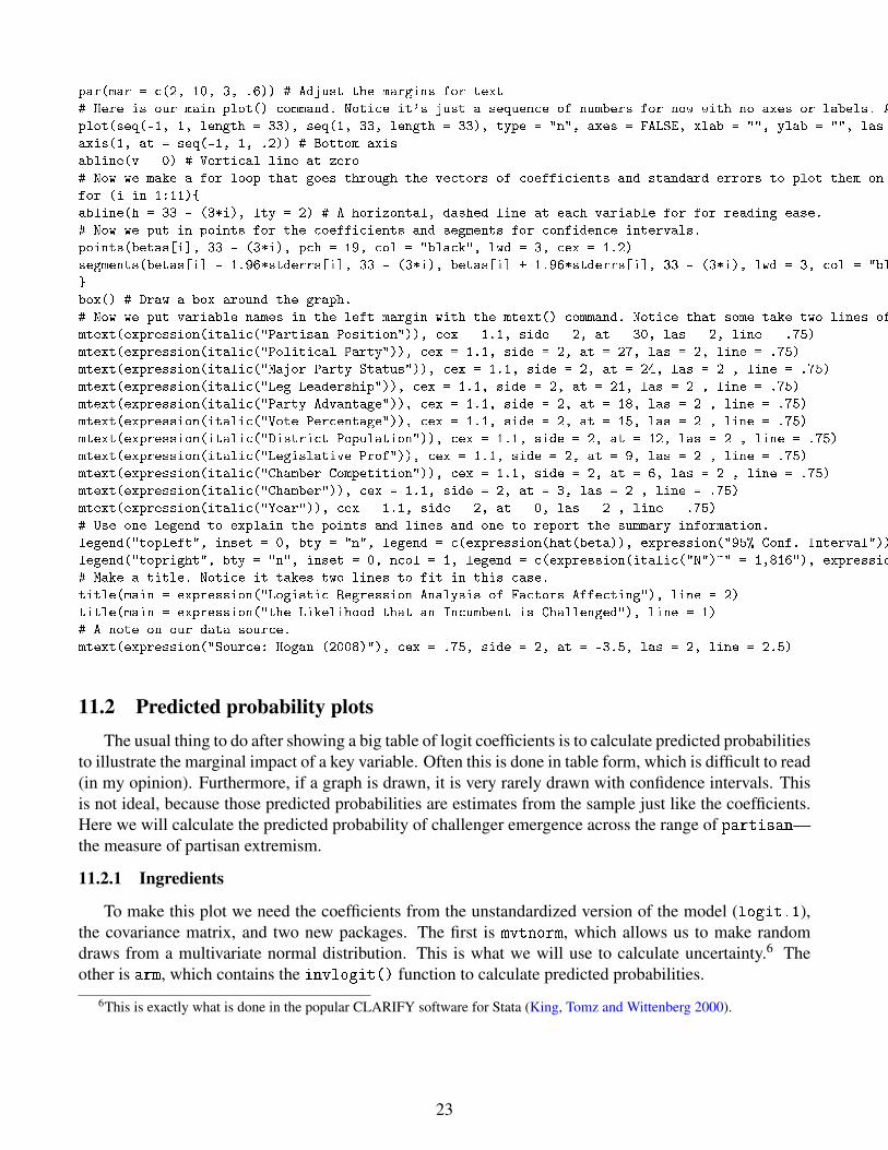
par(mar = c(2, 10, 3, .6)) # Adjust the margins for text

# Here is our main plot() command. Notice it's just a sequence of numbers for now with no axes or labels. All we want to do is define the space.

plot(seq(-1, 1, length = 33), seq(1, 33, length = 33), type = "n", axes = FALSE, xlab = "", ylab = "", las = 2, ylim = c(0, 36))

axis(1, at = seq(-1, 1, .2)) # Bottom axis

abline(v = 0) # Vertical line at zero

# Now we make a for loop that goes through the vectors of coefficients and standard errors to plot them on the graph.

for (i in 1:11){

abline(h = 33 - (3*i), lty = 2) # A horizontal, dashed line at each variable for for reading ease.

# Now we put in points for the coefficients and segments for confidence intervals.

points(betas[i], 33 - (3*i), pch = 19, col = "black", lwd = 3, cex = 1.2)

segments(betas[i] - 1.96*stderrs[i], 33 - (3*i), betas[i] + 1.96*stderrs[i], 33 - (3*i), lwd = 3, col = "black")

}

box() # Draw a box around the graph.

# Now we put variable names in the left margin with the mtext() command. Notice that some take two lines of text.

mtext(expression(italic("Partisan Position")), cex = 1.1, side = 2, at = 30, las = 2, line = .75)

mtext(expression(italic("Political Party")), cex = 1.1, side = 2, at = 27, las = 2, line = .75)

mtext(expression(italic("Major Party Status")), cex = 1.1, side = 2, at = 24, las = 2 , line = .75)

mtext(expression(italic("Leg Leadership")), cex = 1.1, side = 2, at = 21, las = 2 , line = .75)

mtext(expression(italic("Party Advantage")), cex = 1.1, side = 2, at = 18, las = 2 , line = .75)

mtext(expression(italic("Vote Percentage")), cex = 1.1, side = 2, at = 15, las = 2 , line = .75)

mtext(expression(italic("District Population")), cex = 1.1, side = 2, at = 12, las = 2 , line = .75)

mtext(expression(italic("Legislative Prof")), cex = 1.1, side = 2, at = 9, las = 2 , line = .75)

mtext(expression(italic("Chamber Competition")), cex = 1.1, side = 2, at = 6, las = 2 , line = .75)

mtext(expression(italic("Chamber")), cex = 1.1, side = 2, at = 3, las = 2 , line = .75)

mtext(expression(italic("Year")), cex = 1.1, side = 2, at = 0, las = 2 , line = .75)

# Use one legend to explain the points and lines and one to report the summary information.

legend("topleft", inset = 0, bty = "n", legend = c(expression(hat(beta)), expression("95% Conf. Interval")), lwd = 3, pch = c(19, -1), lty = c(-1, 1), bg = "white", cex = 1.25)

legend("topright", bty = "n", inset = 0, ncol = 1, legend = c(expression(italic("N")~" = 1,816"), expression("AIC = 1656.7")), cex = 1.25)

# Make a title. Notice it takes two lines to fit in this case.

title(main = expression("Logistic Regression Analysis of Factors Affecting"), line = 2)

title(main = expression("the Likelihood that an Incumbent is Challenged"), line = 1)

# A note on our data source.

mtext(expression("Source: Hogan (2008)"), cex = .75, side = 2, at = -3.5, las = 2, line = 2.5)

11.2 Predicted probability plotsThe usual thing to do after showing a big table of logit coefficients is to calculate predicted probabilities

to illustrate the marginal impact of a key variable. Often this is done in table form, which is difficult to read(in my opinion). Furthermore, if a graph is drawn, it is very rarely drawn with confidence intervals. Thisis not ideal, because those predicted probabilities are estimates from the sample just like the coefficients.Here we will calculate the predicted probability of challenger emergence across the range of partisan—the measure of partisan extremism.

11.2.1 Ingredients

To make this plot we need the coefficients from the unstandardized version of the model (logit.1),the covariance matrix, and two new packages. The first is mvtnorm, which allows us to make randomdraws from a multivariate normal distribution. This is what we will use to calculate uncertainty.6 Theother is arm, which contains the invlogit() function to calculate predicted probabilities.

6This is exactly what is done in the popular CLARIFY software for Stata (King, Tomz and Wittenberg 2000).

23

11.2.2 Making the plot

Our strategy has a few steps. First, we are going to simulate 100 sets of coefficients from the model.This means we will set the actual coefficient and variance estimates in logit.1 as the mean and covariancematrix of a multivariate normal and take 100 random draws.

library(mvtnorm) # This package draws from multivariate distributions.

library(arm) # This package has the invlogit() function we need.

sims <- 100 # We will simulate 100 coefficients.

pp.sim <- rmvnorm(sims, logit.1$coef, vcov(logit.1))

Next, we will hold all of the variables except partisan to their means and set partisan to its mini-mum. Then we will calculate the predicted probability at these values for all of the 100 sets of simulatedcoefficients. This will produce 100 predicted probabilities, with the mean representing the point estimateand the 2.5th and 97.5th percentiles representing the 95% confidence bounds. We will store this informa-tion, then increment the value of partisan up slightly (in the object called ruler) and do the predictedprobability calculations again for that new value of partisan, holding everything else the same. We willdo this until we reach the maximum value of partisan.

calc <- 50 # Number of times the predicted probability will be calculated.

# Next make the sequence going across the range of partisan. This will become the

# x-axis at the end.

ruler <- seq(min(hogan$partisan), max(hogan$partisan), length = calc)

pe <- numeric(calc) # Empty vectors to store the point estimates and confidence intervals.

lo <- numeric(calc)

hi <- numeric(calc)

for(i in 1:calc){ # First for loop goes across the x-axis values (ruler).

pp <- numeric(sims) # Empty vector to store the actual calculations at each point

# along the x-axis (ruler).

for(j in 1:sims){ # Now loop through all the simulated coefficients and each time

# calculate the predicted probability with partisan set to the current value on

# the x-axis (ruler) and everything else at its mean.

pp[j] <- pp.sim[j, 1] + pp.sim[j, 2]*ruler[i] + pp.sim[j, 3]*mean(hogan$politica) +

pp.sim[j, 4]*mean(hogan$majorpar) + pp.sim[j, 5]*mean(hogan$legisl_a)

} # End calculation loop

pe[i] <- mean(invlogit(pp)) # Point estimate on the probability scale.

lo[i] <- quantile(invlogit(pp), .025)# CIs on the probability scale.

hi[i] <- quantile(invlogit(pp), .975)

} # End x-axis loop (ruler)

Finally, we plot ruler, our range of the variable partisan, on the x-axis and the point estimate andconfidence bounds on the y-axis.

# Now we plot the observed range of partisan (ruler) on the x-axis and the point estimate

# and confidence intervals

plot(ruler, pe, type = "l", lwd = 2, col = "black", ylim = c(0, 1), axes = FALSE,

xlab = "", ylab = "")

lines(ruler, lo, lwd = 2, lty = 2, col = "black")

lines(ruler, hi, lwd = 2, lty = 2, col = "black")

24

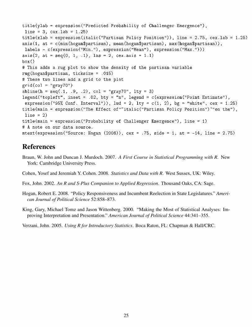
title(ylab = expression("Predicted Probability of Challenger Emergence"),

line = 3, cex.lab = 1.25)

title(xlab = expression(italic("Partisan Policy Position")), line = 2.75, cex.lab = 1.25)

axis(1, at = c(min(hogan$partisan), mean(hogan$partisan), max(hogan$partisan)),

labels = c(expression("Min."), expression("Mean"), expression("Max.")))

axis(2, at = seq(0, 1, .1), las = 2, cex.axis = 1.1)

box()

# This adds a rug plot to show the density of the partisan variable

rug(hogan$partisan, ticksize = .015)

# These two lines add a grid to the plot

grid(col = "gray70")

abline(h = seq(.1, .9, .2), col = "gray70", lty = 3)

legend("topleft", inset = .02, bty = "n", legend = c(expression("Point Estimate"),

expression("95% Conf. Interval")), lwd = 2, lty = c(1, 2), bg = "white", cex = 1.25)

title(main = expression("The Effect of"~italic("Partisan Policy Position")~"on the"),

line = 2)

title(main = expression("Probability of Challenger Emergence"), line = 1)

# A note on our data source.

mtext(expression("Source: Hogan (2008)), cex = .75, side = 1, at = -14, line = 2.75)

ReferencesBraun, W. John and Duncan J. Murdoch. 2007. A First Course in Statistical Programming with R. New

York: Cambridge University Press.

Cohen, Yosef and Jeremiah Y. Cohen. 2008. Statistics and Data with R. West Sussex, UK: Wiley.

Fox, John. 2002. An R and S-Plus Companion to Applied Regression. Thousand Oaks, CA: Sage.

Hogan, Robert E. 2008. “Policy Responsiveness and Incumbent Reelection in State Legislatures.” Ameri-can Journal of Political Science 52:858–873.

King, Gary, Michael Tomz and Jason Wittenberg. 2000. “Making the Most of Statistical Analyses: Im-proving Interpretation and Presentation.” American Journal of Political Science 44:341–355.

Verzani, John. 2005. Using R for Introductory Statistics. Boca Raton, FL: Chapman & Hall/CRC.

25