INTRODUCTION TO QCD

Michelangelo L. Mangano

CERN, TH Division, Geneva, Switzerland

AbstractI review in this series of lectures the basics of perturbative quantum chromody-namics and some simple applications to the physics of high-energy collisions.

1. INTRODUCTION

Quantum Chromodynamics (QCD) is the theory of strong interactions. It is formulated in terms ofelementary fields (quarks and gluons), whose interactions obey the principles of a relativistic QFT, witha non-abelian gauge invariance SU(3). The emergence of QCD as theory of strong interactions could bereviewed historically, analyzing the various experimental data and the theoretical ideas available in theyears 1960–1973 (see e.g. Refs. [17,18]). To do this accurately and usefully would require more timethan I have available. I therefore prefer to introduce QCD right away, and to use my time in exploringsome of its consequences and applications. I will therefore assume that you all know more or less whatQCD is! I assume you know that hadrons are made of quarks, that quarks are spin-1/2, colour-tripletfermions, interacting via the exchange of an octet of spin-1 gluons. I assume you know the concept ofrunning couplings, asymptotic freedom and of confinement. I shall finally assume that you have somefamiliarity with the fundamental ideas and formalism of QED: Feynman rules, renormalization, gaugeinvariance.

If you go through lecture series on QCD (e.g., the lectures given in previous years at the CERNSummer School, Refs. [9–11]), you will hardly ever find the same item twice. This is because QCDtoday covers a huge set of subjects and each of us has his own concept of what to do with QCD andof what are the “fundamental” notions of QCD and its “fundamental” applications. As a result, youwill find lecture series centred around non-perturbative applications, (lattice QCD, sum rules, chiralperturbation theory, heavy quark effective theory), around formal properties of the perturbative expansion(asymptotic behaviour, renormalons), techniques to evaluate complex classes of Feynman diagrams, orphenomenological applications of QCD to possibly very different sets of experimental data (structurefunctions, deep-inelastic scattering (DIS) sum rules, polarized DIS, small x physics (including hardpomerons, diffraction), LEP physics, pp collisions, etc.

I can anticipate that I will not be able to cover or to simply mention all of this. After introducingsome basic material, I will focus on some elementary applications of QCD in high-energy e+e−, ep andpp collisions. The outline of these lectures is the following:

1. Gauge invariance and Feynman rules for QCD.

2. Renormalization, running coupling, renormalization group invariance.

3. QCD in e+e− collisions: from quarks and gluons to hadrons, jets, shape variables.

4. QCD in lepton-hadron collisions: DIS, parton densities, parton evolution.

5. QCD in hadron-hadron collisions: formalism, W/Z production, jet production.

Given the large number of papers which contributed to the development of the field, it is impossible toprovide a fair bibliography. I therefore limit my list of references to some excellent books and reviewarticles covering the material presented here, and more. Papers on specific items can be easily found byconsulting the standard hep-th and hep-ph preprint archives.

41

2. QCD FEYNMAN RULES

There is no free lunch, so before starting with the applications, we need to spend some time developingthe formalism and the necessary theoretical ideas. I will dedicate to this purpose the first two lectures.Today, I concentrate on Feynman rules. I will use an approach which is not canonical, namely it doesnot follow the standard path of the construction of a gauge invariant Lagrangian and the derivation ofFeynman rules from it. I will rather start from QED, and empirically construct the extension to a non-Abelian theory by enforcing the desired symmetries directly on some specific scattering amplitudes.Hopefully, this will lead to a better insight into the relation between gauge invariance and Feynmanrules. It will also provide you with a way of easily recalling or checking your rules when books are notaround!

2.1. Summary of QED Feynman rules

We start by summarizing the familiar Feynman rules for Quantum Electrodynamics (QED). They areobtained from the Lagrangian:

L = ψ(i∂/−m)ψ − eψA/ψ − 1

4FµνF

µν , (1)

where ψ is the electron field, of mass m and coupling constant e, and F µν is the electromagnetic fieldstrength.

Fµν = ∂µAν − ∂νAµ . (2)

The resulting Feynman rules are summarized in the following table:

=i

p/−m+ iε= i

p/+m

p2 −m2 + iε(3)

= −i gµν

p2 + iε(Feynman gauge) (4)

= −ieγµQ (Q = −1 for the electron, Q = 2/3 for the u-quark, etc.)

(5)

Let us start by considering a simple QED process, e+e− → γγ (for simplicity we shall always as-sume m = 0):

= D1 +D2 (6)

The total amplitude Mγ is given by:i

e2Mγ ≡ D1 +D2 = v(q) ε/2

1

q/− k/1

ε/1 u(q) + v(q)ε/1

1

q/− k/2

ε/2 n(q) ≡Mµνεµ1ε

ν2 . (7)

Gauge invariance demands thatεν2∂

µMµν = εµ1∂νMµν = 0 . (8)

Mµ ≡ Mµνεν2 is in fact the current that couples to the photon k1. Charge conservation re-

quires ∂µMµ = 0:

∂µMµ = 0 ⇒ d

dt

∫

M0d3x =

∫

∂0M0 d3x

42

=

∫

~∇ · ~M d3x =

∫

S→∞~M · d~Σ = 0 . (9)

In momentum space, this meanskµ1Mµ = 0 . (10)

Another way of saying this is that the theory is invariant if εµ(k) → εµ(k)+f(k) kµ . This is the standardAbelian gauge invariance associated to the vector potential transformations:

Aµ(x) → Aµ(x) + ∂µf(x) . (11)

Let us verify that Mγ is indeed gauge invariant. Using q/u(q) = v(q)q/ = 0 from the Diracequation, we can rewrite kµ

1Mµ as:

kµ1 ε

ν2Mµν = v(q)ε/2

1

q/− k/1

(k/1 − q/)u(q) + v(q)(k/1 − q)1

k1 − qε/2u(q)

= −v(q)ε/2u(q) + v(q)ε/2u(q) = 0 . (12)

Notice that the two diagrams are not individually gauge invariant, only the sum is. Notice also that thecancellation takes place independently of the choice of ε2. The amplitude is therefore gauge invarianteven in the case of emission of non-transverse photons.

Let us try now to generalize our QED example to a theory where the “electrons” carry a non-Abelian charge, i.e., they transform under a non-trivial representation R of a non-Abelian group G(which, for the sake of simplicity, we shall always assume to be of the SU(N) type. Likewise, weshall refer to the non-abelian charge as “colour”). The standard current operator belongs to the productR⊗ R. The only representation that belongs to R⊗ R for any R is the adjoint representation. Thereforethe field that couples to the colour current must transform as the adjoint representation of the group G.So the only generalization of the photon field to the case of a non-Abelian symmetry is a set of vectorfields transforming under the adjoint of G, and the simplest generalization of the coupling to fermionstakes the form:

= igλaki γ

µmn , (13)

where the matrices λa represent the algebra of the group on the representation R. By definition, theysatisfy the algebra:

[λa, λb] = ifabcλc (14)

for a fixed set of structure constants f abc, which uniquely characterize the algebra. We shall call quarks(q) the fermion fields in R and gluons (g) the vector fields which couple to the quark colour current.

The non-abelian generalization of the e+e− → γγ process is the qq → gg annihilation. Itsamplitude can be evaluated by including the λ matrices in Eq. (6):

i

e2Mγ → i

g2Mg ≡ (λbλa)ij D1 + (λaλb)ij D2 (15)

with (a, b) colour labels (i.e. group indices) of gluons 1 and 2, (i, j) colour labels of q, q, respectively.Using Eq. (14), we can rewrite (15) as:

Mg = (λaλb)ij Mγ − g2 fabcλcij D1 . (16)

43

If we want the charge associated with the group G to be conserved, we still need to demand

kµ1 ε

ν2 M

µνg = εµ1k

ν2 M

µνg = 0 . (17)

Substituting εµ1 → kµ1 in (16) we get instead, using (12):

k1 µMµg = −g2fabc λc

ij vi(q) ε/2ui(q) . (18)

The gauge cancellation taking place in QED between the two diagrams is spoiled by the non-Abeliannature of the coupling of quarks to gluons (i.e., λa and λb do not commute, and f abc 6= 0).

The only possible way to solve this problem is to include additional diagrams. That new interac-tions should exist is by itself a reasonable fact, since gluons are charged (i.e., they transform under thesymmetry group) and might want to interact among themselves. If we rewrite (18) as follows:

k1 µMµg = i

(

fabc g εµ2

)

×(

i g λcij v(q) γµ u(q)

)

, (19)

we can recognize in the second factor the structure of the qqg vertex. The first factor has the appropriatecolour structure to describe a triple-gluon vertex, with a, b, c the colour labels of the three gluons:

= g fabc Vµ1µ2µ3(k1, k2, k3) . (20)

Equation (19) therefore suggests the existence of a coupling like (20), with a Lorentz structure Vµ1µ2µ3

to be specified, giving rise to the following contribution to qq → gg:

= −i g2D3 = (ig λaij)v(q)i γ

µ u(q)j

(−ip2

)

g fabc Vµνρ(−p, k1, k2) εν1(k1) ε

ρ2(k2) . (21)

We now need to find Vµ1µ2µ3(p1, p2, p3) and to verify that the contribution of the new diagram to k1 ·Mg

cancels that of the first two diagrams. We will now show that the constraints of Lorentz invariance, Bosesymmetry and dimensional analysis uniquely fix V , up to an overall constant factor.

Dimensional analysis fixes the coupling to be linear in the gluon momenta. This is because eachvector field carries dimension 1, there are three of them, and the interaction must have total dimensionequal to 4. So at most one derivative (i.e. one power of momentum) can appear at the vertex. In priciple, ifsome mass parameter were available, higher derivatives could be included, with the appropriate powers ofthe mass parameter appearing in the denominator. This is however not the case. It is important to remarkthat the absence of interactions with higher number of derivatives is also crucial for the renormalizabilityof the interaction.

Lorentz invariance requires then that V be built out of terms of the form gµ1µ2pµ3 . Bose symmetryrequires V to be fully antisymmetric under the exchange of any pair (µi, pi) ↔ (µj , pj) since the colourstructure fabc is totally antisymmetric. As a result, for example, a term like gµ1µ2p

µ33 vanishes under

antisymmetrization, while gµ1µ2pµ31 doesn’t. Starting from this last term, we can easily add the pieces

required to obtain the full antisymmetry in all three indices. The result is unique, up to an overall factor:

Vµ1µ2µ3 = V0 [(k1 − k2)µ3gµ1µ2 + (k2 − k3)

µ1gµ2µ3 + (k3 − k1)µ2gµ1µ3 ] . (22)

44

To test the gauge variation of the contribution D3, we set µ3 = µ, ε1 = k1 and k3 = −(k1 + k2) inEq. (21), and we get:

kµ11 εµ2

2 Vµ1µ2µ(k1, k2, k3) = V0 −(k1 + k2)µ(k1 · ε2) + 2(k1 · k2)ε

µ2 − (k2 · ε2)kµ

1 . (23)

The gauge variation is therefore:

k1 ·D3 = g2fabcλcV0

[

v(q)ε/2u(q) −k2 · ε22k1k2

v(q)k/1u(q)

]

. (24)

The first term cancels the gauge variation of D1 +D2 provided V0 = 1, the second term vanishes for aphysical gluon k2, since in this case k2 · ε2 = 0. D1 +D2 +D3 is therefore gauge invariant but, contraryto the case of QED, only for physical external on-shell gluons.

Having introduced a three-gluon coupling, we can induce processes involving only gluons, suchas gg → gg:

(25)

Once more it is necessary to verify the gauge invariance of this amplitude. It turns out that one morediagram is required, induced by a four-gluon vertex. Lorentz invariance, Bose symmetry and dimensionalanalysis uniquely determine once again the structure of this vertex. The overall factor is fixed by gaugeinvariance. The resulting Feynman rule for the 4-gluon vertex is given in Fig. 1.

You can verify that the 3- and 4-gluon vertices we introduced above are exactly those which arisefrom the Yang–Mills Lagrangian:

LY M = −1

4

∑

a

F aµνF

aµν with F aµν = ∂[µA

aν] − g fabcAb

[µAcν] . (26)

It can be shown that the 3- and 4-gluon vertices we generated are all is needed to guarantee gaugeinvariance even for processes more complicated than those studied in the previous simple examples. Inother words, no extra 5- or more gluon vertices have to be introduced to achieve the gauge invarianceof higher-order amplitudes. At the tree level this is the consequence of dimensional analysis and of thelocality of the couplings (no inverse powers of the momenta can appear in the Lagrangian). At the looplevel, these conditions are supplemented by the renormalizability of the theory [3,7].

Before one can start calculating cross-sections, a technical subtlety that arises in QCD when squar-ing the amplitudes and summing over the polarization of external states needs to be discussed. Let usagain start from the QED example. Let us focus, for example, on the sum over polarizations of photon k1:

∑

ε1

|M |2 =

(∑

ε1

εµ1εν∗1

)

MµM∗ν . (27)

The two independent physical polarizations of a photon with momentum k = (k0; 0, 0, k0) are given byεµL,R = (0; 1,±i, 0)/

√2. They satisfy the standard normalization properties:

εL · ε∗L = −1 = εR · ε∗R εL · ε∗R = 0 .

45

= δab −i gαβ

p2 + iε(Feynman gauge)

= δab i

p2 + iε

= δik i

/p−m+ iε

∣∣∣∣mn

= gfabc[

gαβ(p− q)γ + gβγ(q − r)α + gγα(r − p)β]

= −ig2fxacfxbd(

gαβgγδ − gαδgβγ)

−ig2fxadfxbc(

gαβgγδ − gαγgβδ)

−ig2fxabfxcd(

gαγgβδ − gαδgβγ)

= −gfabc qα

= ig λaki γ

αmn

Fig. 1: Feynman rules for QCD. The solid lines represent the femions, the curly lines the gluons, and the dotted lines represent

the ghosts.

46

We can write the sum over physical polarizations in a convenient form by introducing the vector k =(k0; 0, 0,−k0):

∑

i=L,R

εµi εν∗i ≡

0 ~01 0 0

~0 0 1 00 0 0

= −gµν +kµkν + kν kµ

k · k . (28)

We could have written the sum over physical polarizations using any other momentum `µ, providedk · ` 6= 0. This would be equivalent to a gauge transformation (prove it as an exercise). In QEDthe second term in Eq. (28) can be safely dropped, since kµM

µ = 0. As a cross check, notice thatkµM

µ = 0 implies M0 = M3, and therefore:

∑

i=L,R

|εi ·M |2 = |M1|2 + |M2|2 = |M1|2 + |M2|2 + |M3|2 − |M0|2 ≡ −gµν MµM∗ν . (29)

Therefore, the production of the longitudinal and time-like components of the photon cancel each other.This is true regardless of whether additional external photons are physical or not, since the gauge in-variance k1 ·M = 0 shown in Eq. (12) holds regardless of the choice for ε2, as already remarked. Inparticular,

kµ11 kµ2

2 Mµ1µ2 = 0 (30)

(for n photons, kµ11 kµ2

2 . . . kµnn Mµ1 ...µn = 0) and the production of any number of unphysical photons

vanishes. The situation in the case of gluon emission is different, since k1 ·M ∝ ε2 · k2, which vanishesonly for a physical ε2. This implies that the production of one physical and one non-physical gluons isequal to 0, but the production of a pair of non-physical gluons is allowed! If ε2 · k2 6= 0, then M0 is notequal to M3, and Eq. (28) is not equivalent to

∑εµε

∗ν = −gµν .

Exercise: show that

∑

non−physical

|εµ1 εν2Mµν |2 =

∣∣∣∣i g

2 fabcλc 1

2k1k2v(q)k1/ u(q)

∣∣∣∣

2

. (31)

In the case of non-Abelian theories, it is therefore important to restrict the sum over polarizations and(because of unitarity) the off-shell propagators to physical degrees of freedom with the choice of physicalgauges. Alternatively, one has to undertake a study of the implications of gauge-fixing in non-physicalgauges for the quantization of the theory (see Refs. [3,7]). The outcome of this analysis is the appearanceof two colour-octet scalar degrees of freedom (called ghosts) whose role is to enforce unitarity in non-physical gauges. They will appear in internal closed loops, or will be pair-produced in final states.They only couple to gluons. Their Feynman rules are supplemented by the prescription that each closedloop should come with a −1 sign, as if they obeyed Fermi statistics. Being scalars, this prescriptionbreaks the spin-statistics relation, and leads as a result to the possibility that production probabilitiesbe negative. This is precisely what is required to cancel the contributions of non-transverse degrees offreedom appearing in non-physical gauges. Adding the ghosts contribution to qq → gg decays (usingthe Feynman rules from Fig. 1) gives in fact

= −∣∣∣∣i g2 fabcλc 1

2k1k2v(q)k1/ u(q)

∣∣∣∣

2

, (32)

which exactly cancels the contribution of non-transverse gluons in the non-physical gauge∑εµε

∗ν =

−gµν , given in Eq. 31.

47

The detailed derivation of the need for and properties of ghosts (including their Feynman rulesand the “−1” prescription for loops) can be found in the suggested textbooks. I will not derive theseresults here since we will not need them for our applications (we will use physical gauges or will con-sider processes not involving the 3g vertex). The full set of Feynman rules for the QCD Lagrangian isgiven in Fig. 1.

2.2. Some useful results in colour algebra

The presence of colour factors in the Feynman rules makes it necessary to develop some technology toevaluate the colour coefficients which multiply our Feynman diagrams. To be specific, we shall assumethe gauge group is SU(N). The fundamental relation of the algebra is

[λa, λb] = ifabdλc , (33)

with fabc totally antisymmetric. This relation implies that all λ matrices are traceless. For practicalcalculations, since we will always sum over initial, final, and intermediate state colours, we will neverneed the explicit values of f abc. All of the results can be expressed in terms of group invariants (a.k.a.Casimirs), some of which we will now introduce. The first such invariant (TF ) is chosen to fix thenormalization of the matrices λ:

tr(λaλb) = TF δab , (34)

where by convention TF = 1/2 for the fundamental representation. Should you change this convention,you would need to change the definition (i.e. the numerical value) of the coupling constant g, since g λa

appears in the Lagrangian and in the Feynman rules.

Exercise: Show that tr(λaλb) is indeed a group invariant. Hint: write the action on λa of a general grouptransformation with infinitesimal parameters εb as follows:

δλa =∑

b,c

εbfabcλc . (35)

The definition of TF allows to evaluate the colour factor for an interesting diagram, i.e. the quarkself-energy:

∼∑

a

(λaλa)ij ≡ CF δij . (36)

The value of CF can be obtained by tracing the relation above:

CFN = tr∑

a

λaλa = δab TF δab =N2 − 1

2, (37)

where we used the fact that δabδab = N2 − 1, the number of matrices λa (and of gluons) for SU(N).

There are some useful graphical tricks (which I learned from P. Nason, Ref. [9]) which can be usedto evaluate complicated expressions. The starting point is the following representation for the quark andgluon propagators, and for the qqg and ggg interaction vertices:

fermion (38)

gluon (39)

48

1√2

− 1

N

Fermion-Gluon Vertex (ta) (40)

1√2

−

3-Gluon Vertex (f abc) (41)

Contraction over colour indices is obtained by connecting the respective colour (or anticolour) lines. Aclosed loop of a colour line gives rise to a factor N , since the closed loop is equivalent to the trace of theunit matrix. So the above representation of the qqg vertex embodies the idea of “colour conservation”,whereby the colour-anticolour quantum numbers carried by the qq pair are transferred to the gluon.The piece proportional to 1/N in the qqg vertex appears only when the colour of the quark and of theantiquark are the same. It ensures that λa is traceless, as it should. This can be easily checked as anexercise. The factor 1/

√2 is related to the chosen normalization of TF .

As a first example of applications, let us reevaluate CF :

=1√2

− 1

N

× 1√2

− 1

N

=1

2

− 1

N− 1

N+

+1

N2

= δijN2 − 1

2N. (42)

As an exercise, you can calculate the colour factor for qq → qq scattering, and show that:

∑

a

(λa)ij(λa)`k = =

1

2

− 1

N

=1

2

(

δikδ`j −1

Nδijδ`k

)

. (43)

This result can be used to evaluate the one-loop colour factors for the interaction vertex with a photon:

=1

2

− 1

N

=

1

2

N2 − 1

Nδij = CF δij . (44)

49

For the interaction with a gluon we have instead:

=1√2

− 1

N

× 1

2

− 1

N

=1

2√

2

− 1

N− 1

N+

1

N2

= − 1

2N

1√2

− 1

N

= − 1

2N(45)

Notice that in the case of the coupling to the photon the qq pair is in a colour-singlet state. The gluonexchange effect in this case has a positive sign (⇒ attraction). In the case of the coupling to the gluonthe qq pair is in a colour-octet state, and the gluon-exchange correction has a negative sign relative to theBorn interaction. The force between a qq pair is therefore attractive if the pair is in a colour-singlet, whileit is repulsive if it is in a colour-octet state! This gives a qualitative argument for why no colour-octet qqbound state exists.

The remaining important relation that one needs is the following:

∑

a,b

fabcfabd = CAδcd with CA = N . (46)

You can easily prove it by using the graphical representation given in Eq. (41), or by using Eq. (43)and fabc = −2i tr([λa, λb]λc).

3. RENORMALIZATION, OR: “THEORISTS ARE NOT AFRAID OF INFINITIES!”

QCD calculations are extremely demanding. Although perturbative, the size of the coupling constanteven at rather large values of the exchanged momentum, Q2, is such that the convergence of the pertur-bative expansion is slow. Several orders of perturbation theory (PT) are required in order to obtain a goodaccuracy. The complexity of the calculations grows dramatically with the order of the approximation. Asan additional complication, the evaluation of a large class of higher-order diagrams gives rise to resultswhich are a priori ill-defined, namely to infinities. A typical example of what is known as an ultravioletdivergence, appears when considering the corrections to the quark self-energy. Using the Feynman rulespresented in the previous lecture, one can obtain:

= (−ig)2 CF

∫d4`

(2π)4γµ

i

p/+ `γν

(

− igµν

`2

)

≡ip/Σ(p) , (47)

where simple manipulations lead to the following expression for Σ(p):

Σ(p) = iCF

∫d4`

(2π)41

`2(p+ `)2, (48)

50

which is logarithmically divergent in the ultraviolet (|`| → ∞) region. In this lecture we will discuss howto deal with these infinities. To start with, we study a simple example taken from standard electrostatics.

3.1. The potential of an infinite line of charge

Let us consider a wire of infinite length, carrying a constant charge density λ. By definition, the dimen-sions of λ are [length]−1 . Our goal is to evaluate the electric potential, and eventually the electric field,in a point P at distance R from the wire. There is no need to do any calculation to anticipate that theevaluation of the electric potential will cause some problem. Using the fact that the potential should belinear in the charge density λ, we write V (R) = λf(R). Since the potential itself has the dimensions of[length]−1 , we clearly see that there is no room for f(R) to have any non-trivial functional dependenceon R. The problem is made explicit if we try to evaluate V (R) using the standard EM formulas:

V (R) =

∫λ(r)

rdx = λ

∫ +∞

−∞

dx√R2 + x2

, (49)

where the integral runs over the position x on the wire. This integral is logarithmically divergent, and thepotential is ill-defined. We know however that this is not a serious issue, since the potential itself is nota physical observable, only the electric field is measurable. Since the electric field is obtained by takingthe gradient of the scalar potential, it will be proportional to

V ′(R) ∼ λ

∫ +∞

−∞

dx

(R2 + x2)3/2, (50)

which is perfectly convergent. It is however interesting to explore the possibiity of providing a usefuloperative meaning to the definition of the scalar potential. To do that, we start by regularizing the integralin Eq. (49). This can be done by introducing the regularized V (R) defined as:

VΛ(R) =

∫ Λ

−Λλ

dx√R2 + x2

= λ log

[√Λ2 +R2 + Λ√Λ2 +R2 − Λ

]

. (51)

We can then define the electric field as

~E(R) = limΛ→∞

[−~∇VΛ(R)] . (52)

It is easy to check that this prescription leads to the right result:

~E(R) = limΛ→∞

R2λ

R

Λ√Λ2 +R2

→ 2λ

RR . (53)

Notice that in this process we had to introduce a new variable Λ with the dimension of a length. Thisallows us to solve the puzzle first pointed out at the beginning. At the end, however, the dependenceof the physical observable (i.e. the electric field) on this extra parameter disappears. Notice also thatthe object:

δV = limΛ→∞

[VΛ(r2) − VΛ(r1)] = λ log

(

r21r22

)

(54)

is well defined. This suggests a way of defining the potential which is meaninfgul even in the Λ → ∞limit. We can renormalize the potential, by subtracting V (R) at some fixed value of R = R0, and takingthe Λ → ∞ limit:

V (R) → V (R) − V (R0) = λ log

(

R20

R2

)

. (55)

51

The non-physical infinities present in V (R) and V (R0) cancel each other, leaving a finite result, witha non-trivial R-dependence. Once again, this is possible because a dimensionful parameter (in thiscase R0) has been introduced.

This example suggests a strategy for dealing with divergencies:

1. Identify an appropriate way to regularize infinite integrals

2. Absorb the divergent terms into a redefinition of fields or parameters, e.g, via subtractions.This step is usually called renormalization.

3. Make sure the procedure is consistent, by checking that the physical results do not dependon the regularization prescription.

In the rest of this lecture I will explain how this strategy is applied to the case of ultraviolet divergenciesencountered in perturbation theory.

3.2. Dimensional regularization

The typical expressions we have to deal with have the form:

I(M2) =

∫d4`

(2π)41

[`2 +M2]2. (56)

You can easily show that the integral encountered in the quark self-energy diagram can be rewritten as:

1

`21

(`− p)2=

∫ 1

0dx

1

(L2 +M2)2, with L = `− xp,M 2 = x(1 − x)p2 . (57)

The most straighforward extension of the ideas presented above in the case of the infinite charged wire isto regularize the integral using a momentun cutoff, and to renormalize it with a subtraction (for example,I(M2) − I(M2

0 )). Experience has shown, however, that the best way to regularize I(M 2) is to take theanalytic continuation of the integral in the number of space-time dimensions. In fact

ID(M2) =

∫dD`

(2π)D

1

(`2 +M2)2(58)

is finite ∀D < 4. If we could assign a formal meaning to ID(M2) for continuous values of D away fromD = 4, we could then perform all our manipulations in D 6= 4, regulate the divergences, renormalizefields and couplings, and then go back to D = 4.

To proceed, one defines (for Euclidean metrics):

dD` = dΩd−1 `D−1d` , (59)

with dΩD−1 the differential solid angle inD dimensions. ΩD−1 is the surface of aD-dimensional sphere.It can be obtained by using the following formal identity:

∫

dD` e−~2 ≡

[∫

d` e−`2]D

= πD/2 . (60)

The integral can also be evaluated, using Eq. (59), as∫

dD` e−~2

= ΩD

∫ ∞

0`D−1 e−`2d` = ΩD

1

2

∫ ∞

0d`2(`2)

D−22 e−`2

= ΩD1

2

∫ ∞

0dx e−xx

D−22 ≡ ΩD

2Γ

(D

2

)

. (61)

52

Comparing Eqs. (60) and (61) we get:

ID(M2) =1

(4π)D/2

1

Γ(D/2)

∫ ∞

0dx x

D−22 (x+M2)2 =

1

(4π)D/2

Γ(2 −D/2)

Γ(2)(M2)

D2−2 (62)

Defining D = 4 − 2ε (with the understanding that ε will be taken to 0 at the end of the day), and usingthe small-ε expansion:

Γ(ε) =1

ε− γε + O(ε) , (63)

we finally obtain:

(4π)2ID(M2) → 1

ε− log 4πM 2 − γε . (64)

The divergent part of the integral is then regularized as a pole in (D − 4). The M -dependent part ofthe integral behaves logarithmically, as expected because the integral itself was dimensionless in D = 4.The 1/ε pole can be removed by a subtraction:

I(M2) = I(µ2) + (4π)2 log

(

µ2

M2

)

, (65)

where the subtraction scale µ2 is usually referred to as the “renormalization scale”.

One can prove (and you will find this in the quoted textbooks) that other divergent integrals whichappear in other loop diagrams can be regularized in a similar fashion, with the appearance of 1/ε poles.Explicit calculations and more details on this techinque can be found in the literature quoted at the end.

3.3. Renormalization

Let us come back now to our quark self-energy diagram, Eq. (47). After regulating the divergence usingdimensional regularization, we can eliminate it by adding a counterterm to the Lagrangian:

L → L + Σ(p)ψi∂/ψ = [1 + Σ(p)]ψi∂/ψ + . . . (66)

In this way, the corrections at O(g2) to the inverse propagator are finite:

= −ip/Σ(p) + ip/Σ(p) = 0 . (67)

The inclusion of this counterterm can be interpreted as a renormalization of the quark wave function. Tosee this, it is sufficient to define:

ψR =(

1 + Σ(p2))1/2

ψ (68)

and verify that the kinetic part of the Lagrangian written in terms of ψR takes again the canonical form.

It may seem that this regularization/renormalization procedure can always be carried out, with allpossible infinities being removed by ad hoc counterterms. This is not true. That these subtractions can beperformed consistently for any possible type of divergence which develops in PT is a highly non-trivialfact. To convince you of this, consider the following example.

53

Let us study the QCD corrections to the interaction of quarks with a photon:

= (−ig)2CF

∫d4`

(2π)4

γp i

p/+ /

Γµ

︷ ︸︸ ︷

(−i eγµ)i

p/+ /γp

(−i`2

)

= −ig2CF

∫d4`

(2π)4(−2)(p/ + /)Γµ(p/+ /)

1

`2(p+ `)2(p+ `)2

leading div.−→ −ig2(−2)CF

∫d4`

(2π)4/Γµ/

`2(p+ `)2(p+ `)2def= ieγµV (q2) .

It is easily recognized that V (q2) is divergent. The divergence can be removed by adding a countertermto the bare Lagrangian:

Lint = −e Aµψγµψ → −eAµψγ

µψ − eV (q2)Aµψγµψ

= −[1 + V (q2)] e Aµψγµψ . (69)

If we take into account the counterterm that was introduced to renormalize the quark self-energy, the partof the quark Lagrangian describing the interaction with photons is now:

Lq,γ =[

1 + Σ(p2)]

ψ i ∂/ ψ −[

1 + V (q2)]

eAµ ψγµψ . (70)

Defining a renormalized charge by:

eR = e1 + V (p2)

1 + Σ(q2), (71)

we are left with the renormalized Lagrangian:

LR = ψR i ∂/ ψR + eRAµ ψR γµ ψR . (72)

Can we blindly accept this result, regardless of the values of the counterterms V (p2) and Σ(q2)? Theanswer to this question is NO! Charge conservation, in fact, requires eR = e. The electric charge carriedby a quark cannot be affected by the QCD corrections, and cannot be affected by the renormalization ofQCD-induced divergencies. There are many ways to see that if eR 6= e the electric charge would not beconserved in strong interactions. The simplest way is to consider the process e+νe → W+ → ud. Theelectric charge of the initial state is +1 in units of e. After including QCD corrections (which in the caseof the interaction with a W are the same as those for the interaction of quarks with a photon), the chargeof the final state is +1 in units of eR. Unless eR = e, the total electric charge would not be conserved inthis process! The non-renormalization of the electric charge in presence of strong interactions is the factthat makes the charge of the proton to equal the sum of the charges of its constituent quarks, in spite ofthe complex QCD dynamics that holds the quarks together.

As a result, the renormalization procedure is consistent with charge conservation if and only if

V (q2)

Σ(p2)

q2→0= 1 . (73)

This identity should hold at all orders of perturbation theory. It represents a fundamental constraint onthe consistency of the theory, and shows that the removal of infinities, by itself, is not a trivial trick whichcan be applied to arbitrary theories. Fortunately, the previous identity can be shown to hold. You canprove it explicitly at the one-loop order by explicitly evaluating the integrals defining V (q) and Σ(p).

54

To carry out the renormalization program for QCD at 1-loop order, several other diagrams inaddition to the quark self-energy need to be evaluated. One needs the corrections to the gluon self-energy,to the coupling of a quark pair to a gluon, and to the 3-gluon coupling. Each of these corrections gives riseto infinities, which can be regulated in dimensional regularization. For the purposes of renormalization,it is useful to apply the concept of D dimensions not only to the evaluation of the infinite integrals, but tothe full theory as well. In other words we should consider the Lagrangian as describing the interactions offields inD-dimensions. Nothing changes in its form, but the canonical dimensions of fields and couplingswill be shifted. This is because the action (defined as the integral over space-time of the lagrangian), is adimensionless quantity. As a result, the canonical dimensions of the fields, and of the coupling constants,have to depend on D:

[∫

dDxL(x)

]

= 0 ⇒ [L] = D = 4 − 2ε ,

[∂µφ∂µφ] = D ⇒ [φ] = 1 − ε ,

[ψ∂/ψ] = D ⇒ [ψ] = 3/2 − ε ,

[ψA/ψg] = D ⇒ [g] = ε .

The gauge coupling constant acquires dimensions! This is a prelude to the non-trivial behaviour ofthe renormalized coupling constant as a function of the energy scale (“running”). But before we cometo this, let us go back to the calculation of the counter-terms and the construction of the renormalizedLagrangian.

Replace the bare fields and couplings with renormalized ones1:

ψbare = Z1/22 ψR ,

Aµbare = Z

1/23 Aµ

R ,

gbare = Zg µεgR .

We explicitly extracted the dimensions out of gbare, introducing the dimensional parameter µ (renormal-ization scale). In this way the renormalized coupling gR is dimensionless (as it should be once we goback to 4-dimensions).

The Lagrangian, written in terms of renormalized quantities, becomes:

L = Z2ψi∂/ψ − 1

4Z3F

aµνF

µνa + ZgZ2Z

1/23 µε gψA/ψ + (gauge fixing, ghosts, . . .) (74)

It is customary to defineZ1 = Zg Z2 Z

1/23 . (75)

If we set Zn = 1 + δn, we then obtain:

L = ψ i ∂/ψ − 1

4F a

µνFµνa + µε gψA/ψ + [ghosts, GM]

+ δ2 ψ i∂/ψ − 1

4δ3F

aµνF

µνa + δ1µεgψA/ψ . (76)

The counter-terms δi are fixed by requiring the 1-loop Green functions to be finite. The explicit evalua-tion, which you can find carried out in detail, for example, in Refs. [7,3], gives:

1For the sake of simplicity, here and in the following we shall assume the quarks as massless. The inclusion of the massterms does not add any interesting new feature in what follows.

55

quark self-energy ⇒ δ2 = −CF

(αs

4π

1

ε

)

, (77)

gluon self-energy ⇒ δ3 =

(5

3CA − 4

3nf TF

)αs

4π

1

ε, (78)

qqg vertex corrections ⇒ δ1 = −(CA + CF )αs

4π

1

ε. (79)

As usual we introduced the notation αs = g2/4π. The strong-coupling renormalization constant Zg canbe obtained using these results and Eq. (75):

Zg =Z1

Z2Z1/23

= 1 + δ1 − δ2 −1

2δ3 = 1 +

αs

4π

1

ε

[

−11

6CA +

2

3nF TF

]def≡ 1− 1

ε

(b02

)

αs . (80)

Notice the cancellation of the terms proportional to CF , between the quark self-energy (Z2) and theabelian part of the vertex correction (Z1). This is the same as in the case of the QCD non-renormalizationof the electric coupling, discussed at the beginning of the lecture. The non-abelian part of the vertexcorrection contributes viceversa to the QCD coupling renormalization. This is a consequence of gaugeinvariance. The separation of the non-abelian contributions to the self-energy and to the vertex is notgauge-invariant, only their sum is. Notice also that the consistency of the renormalization procedurerequires that the renormalized strong coupling g defining the strength of the interaction of quarks andgluons should be the same as that defining the interaction of gluons among themselves. If this didn’thappen, the gauge invariance of the qq → gg process so painfully achieved in the first lecture by fixingthe coefficient of the 3-gluon coupling would not hold anymore at 1-loop! Once again, this additionalconstraint can be shown to hold through an explicit calculation.

3.4. Running of αs

The running of αs is a consequence of the renormalization-scale independence of the renormalizationprocess. The bare coupling gbare knows nothing about our choice of µ. The parameter µ is an artifactof the regularization prescription, introduced to define the dimensionful coupling in D dimensions, andshould not enter in measurable quantities. As a result:

dgbare

dµ= 0 . (81)

Using the definition of g: gbare = µεZg g, we then get

εµ2ε Z2g αs + µ2ε αs2Zg

dZg

dt+ µ2ε Z2

g

dαs

dt= 0 , (82)

whered

dt= µ2 d

dµ2=

d

d log µ2. (83)

Zg depends upon µ only via the presence of αs. If we define

β(αs) =dαs

dt, (84)

we then get:

β(αs) + 2αs

Zg

dZg

dαsβ(αs) = −εαs . (85)

56

Using Eq. (80) and expanding in powers of αs, we get:

β(αs) =−εαs

1 + 2 αsZg

dZg

dαs

=−εαs

1 − b0αsε

= −b0α2s +O(α2

s, ε) , (86)

and finally:

β(αs) = −b0α2s with b0 =

1

2π

(11

6CA − 2

3nf TF

)

N=3=

1

12π(33 − 2nf ) . (87)

We can now solve Eq. (84), assuming b0 > 0 (which is true provided the number of quark flavours is lessthan 16) and get the famous running of αs:

αs(µ2) =

1

b0 log(µ2/Λ2). (88)

The parameter Λ describes the boundary condition of the first order differential equation defining therunning of αs, and corresponds to the scale at which the coupling becomes infinity.

3.5. Renormalization group invariance

The fact that the coupling constant αs depends on the unphysical renormalizaiton scale µ should not bea source of worry. This is because the coupling constant itself is not an observable. What we observe aredecay rates, spectra, or cross sections. These are given by the product of the coupling constant times somematrix element, which in general will acquire a non-trivial renormalization-scale dependence through therenormalization procedure. We therefore just need to check that the scale dependence of the couplingconstant and of the matrix elements cancel each other, leaving results which do not depend on µ.

Consider now a physical observable, for example the ratio R = σ(e+e− → hadrons)/σ(e+e−

→ µ+µ−). R can be calculated in perturbation theory within QCD, giving rise to an expansion in therenormalized coupling αs(µ):

R[αs, s/µ2] = 1 + αs f1(t) + α2

s f2(t) + . . . =∞∑

n=0

αns f(n)(t) , (89)

where t = s/µ2 (and we omitted a trivial overall factor 3∑

f Q2f ). R depends on µ explicitly via the

functions f(n)(t) and implicitly through αs. Since R is an observable, it should be independent of µ, andthe functions f(n)(t) cannot be totally arbitrary. In particular, one should have:

µ2 dR

dµ2= 0 =

[

µ2 ∂

∂µ2+ β(αs)

∂

∂αs

]

R[αs, s/µ2] = 0 . (90)

Before we give the general, formal solution to this differential equation, it is instructive to work outdirectly its form within perturbation theory.

µ2 dR

dµ2= 0 = β(αs) f1(t) + αs µ

2 df1

dµ2+ 2αs β(αs) f2(t) + α2

s µ2 df2

dµ2+ . . . (91)

At order αs (remember that β is of order α2s) we get

df1

dµ2= 0 ⇒ f1 = constant ≡ a1 . (92)

This is by itself a non-trivial result! It says that the evaluation of R at one-loop is finite, all UV infinitiesmust cancel without charge renormalization. If they didn’t cancel, f1 would depend explicitly on µ. As

57

we saw at the beginning, this is a consequence of the non-renormalization of the electric charge. At orderα2

s we have:

β(αs)f1(t) + α2s

df2

d log µ2= 0 ⇒ f2 = b0 a1 log

µ2

s+ a2 (integration constant) . (93)

So up to order α2s we have:

R = 1 + a1 αs︸ ︷︷ ︸

one−loop

+ a1 b0 α2s log µ2/s+ a2α

2s

︸ ︷︷ ︸

two−loops

+ . . . (94)

Notice that the requirement of renormalization group invariance allows us to know the coefficient of thelogarithimc term at 2-loops without having to carry out the explicit 2-loop calculation! It is also importantto notice that in the limit of high energy, s → ∞, the logarithmic term of the two-loop contributionbecomes very large, and this piece becomes numerically of order αs as soon as log s/µ2 >∼ 1/b0 αs. Youcan easily check that renormalization scale invariance requires the presence of such logs at all orders ofPT, in particular:

f(n)(t) = a1

[

b0 logµ2

s

]n

+ . . . (95)

We can collect all these logs as follows:

R = 1 + a1αs

[

1 + αsbo logµ2

s+ (αsb0 log

µ2

s)2 + . . .

]

+ a2α2s + . . . (96)

= 1 + a1αs(µ)

1 + αs(µ)bo log sµ2

+ a2α2s + . . . ≡ 1 + a1αs(s) + a2α

2s + . . . (97)

In fact:αs(µ)

1 + αs(µ)bo log sµ2

=1

bo log µ2

Λ2 + bo log sµ2

=1

bo log sΛ2

≡ αs(s) (98)

RG invariance constrains the form of higher-order corrections. All of the higher-order logarithmic termsare determined in terms of lower-order finite coefficients. They can be resummed by simply setting thescale of αs to s. You can check by yourself that this will work also for the higher-order terms, such asthose proportional to a2. So the final result has the form:

R = 1 + a1αs(s) + a2α2s(s) + a3α

3s(s) + . . . (99)

Of course a1, a2, . . . have to be determined by an explicit calculation. However, the truncation of theseries at order n has now an accuracy which is truly of order αn+1

s , contrary to before when higher-order terms were as large as lower-order ones. The explicit calculation has been carried out up to the a3

coefficient, in particular,

a1 =3

4

CF

π≡ 1

π. (100)

The formal proof of the previous equation can be obtained by showing that the general form of theequation

[

µ2 ∂

∂µ2+ β(αs)

]

R (αs,s

µ2) = 0 , (101)

is given by

R(αs(s), 1) , with

dαs

d log sµ2

= β(αs) .(102)

58

4. QCD IN e+e− COLLISIONS

e+e− collisions provide one of the cleanest environments in which to study applications of QCD at highenergy. This is the place where theoretical calculations have today reached their best accuracy, and whereexperimental data are the most precise, especially thanks to the huge statistics accumulated by LEP, LEP2and SLC. The key process is the annihilation of the e+e− pair into a virtual photon or Z0 boson, whichwill subsequently decay to a qq pair. e+e− collisions have therefore the big advantage of providing analmost point-like source of quark pairs, so that, contrary to the case of interactions involving hadrons inthe initial state, we at least know very precisely the state of the quarks at the beginning of the interactionprocess.

Nevertheless, it is by no means obvious that this information is sufficient to predict the propertiesof the hadronic final state. We all know that this final state is clearly not simply a qq pair, but some high-multiplicity set of hadrons. It is therefore not obvious that a calculation done using the simple picturee+e− → qq will have anything to do with reality. For example, one may wonder why don’t we needto calculate σ(e+e− → qqg . . . g . . .) for all possible gluon multiplicities to get an accurate estimate ofσ(e+e− → hadrons). And since in any case the final state is not made of q’s and g’s, but of π’s, K’s,ρ’s, etc., why would σ(e+e− → qqg . . . g) be enough?

The solution to this puzzle lies both in a question of time and energy scales, and in the dynamicsof QCD. When the qq pair is produced, the force binding q and q is proportional to αs(s) (

√s being

the e+e− centre-of-mass energy). Therefore it is weak, and q and q behave to good approximation likefree particles. The radiation emitted in the first instants after the pair creation is also perturbative, and itwill stay so until a time after creation of the order of (1 GeV)−1, when radiation with wavelengths >∼ (1GeV)−1 starts being emitted. At this scale the coupling constant is large, non-perturbative phenomenaand hadronization start playing a role. However, as we will show, colour emission during the perturbativeevolution organizes itself in such a way as to form colour-neutral, low mass, parton clusters highlylocalized in phase-space. As a result, the complete colour-neutralization (i.e., the hadronization) doesnot involve long-range interactions between partons far away in phase-space. This is very important,because the forces acting among coloured objects at this time scale would be huge. If the perturbativeevolution were to separate far apart colour-singlet qq pairs, the final-state interactions taking place duringthe hadronization phase would totally upset the structure of the final state. As an additional result of this“pre-confining” evolution, memory of where the local colour-neutral clusters came from is totally lost. Sowe expect the properties of hadronization to be universal: a model that describes hadronization at a givenenergy will work equally well at some other energy. Furthermore, so much time has passed since theoriginal qq creation, that the hadronization phase cannot significantly affect the total hadron productionrate. Perturbative corrections due to the emission of the first hard partons should be calculable in PT,providing a finite, meaningful cross-section.

The nature of non-perturbative corrections to this picture can be explored. One can prove for ex-ample that the leading correction to the total rateRe+e− is of order F/s2, where F ∝ 〈0|αsF

aµνF

µνa|0〉 isthe so-called gluon condensate. Since F ∼ O(1 GeV4), these NP corrections are usually very small. Forexample, they are of O(10−8) at the Z0 peak! Corrections scaling like Λ2/s or Λ/

√s can nevertheless

appear in other less inclusive quantities, such as event shapes or fragmentation functions.

We now come back to the perturbative evolution, and will devote the first part of this lectureto justifying the picture given above. In the second half we shall discuss jet cross-sections and shapevariables.

59

4.1. Soft gluon emission

Emission of soft gluons plays a fundamental role in the evolution of the final state [6,15]. Soft gluons areemitted with large probability, since the emission spectrum behaves like dE/E, typical of bremstrahlungeven in QED. They provide the seed for the bulk of the final-state multiplicity of hadrons. The study ofsoft-gluon emission is simplified by the simplicity of their couplings. Being soft (i.e., long wavelength)they are insensitive to the details of the very-short-distance dynamics: they cannot distinguish features ofthe interactions which take place on time scales shorter than their wavelength. They are also insensitiveto the spin of the partons: the only feature they are sensitive to is the colour charge. To prove this let usconsider soft-gluon emission in the qq decay of an off-shell photon:

(103)

Asoft = u(p)ε(k)(ig)−ip/+ k/

Γµ v(p) λaij + u(p) Γµ i

p/+ k/(ig)ε(k) v(p) λa

ij

=

[g

2p · k u(p)ε(k) (p/ + k/)Γµ v(p) − g

2p · k u(p) Γµ (p/+ k/)ε(k) v(p)

]

λaij .

I used the generic symbol Γµ to describe the interaction vertex with the photon to stress the fact that thefollowing manipulations are independent of the specific form of Γµ. In particular, Γµ can represent anarbitrarily complicated vertex form factor. Neglecting the factors of k/ in the numerators (since k p, p,by definition of soft) and using the Dirac equations, we get:

Asoft = gλaij

(p · εp · k − pε

p · k

)

ABorn . (104)

We then conclude that soft-gluon emission factorizes into the product of an emission factor, times theBorn-level amplitude. From this exercise, one can extract general Feynman rules for soft-gluon emission:

= g λaij 2pµ (105)

Exercise: Derive the g → gg soft-emission rules:

= igfabc 2pµ gνρ (106)

Example: Consider the “decay” of a virtual gluon into a quark pair. One more diagram should beadded to those considered in the case of the electroweak decay. The fact that the quark pair is not in acolour-singlet state anymore makes things a bit more interesting:

60

(107)

k→0=

[

i g fabc λcij

(Qε

Qk

)

+ g (λb λa)ij

(pε

pk

)

− g (λaλb)ij

(pε

pk

) ]

ABorn

= g (λa λb)ij

[Qε

Qk− pε

pk

]

+ g (λb λa)ij

[pε

pk− Qε

Qk

]

. (108)

The two factors correspond to the two possible ways colour can flow in this process:

(109)

In the first case the antiquark (colour label j) is colour connected to the soft gluon (colour label b),and the quark (colour label i) is connected to the decaying gluon (colour label a). In the second case,the order is reversed. The two emission factors correspond to the emission of the soft gluon from theantiquark, and from the quark line, respectively. When squaring the total amplitude, and summing overinitial and final-state colours, the interference between the two pieces is suppressed by 1/N 2 relative tothe individual squares:

∑

a,b,i,j

|(λaλb)ij |2 =∑

a,b

tr(

λaλbλbλa)

=N2 − 1

2CF = O(N3) , (110)

∑

a,b,i,j

(λaλb)ij [(λbλa)ij]

∗ =∑

a,b

tr(λaλbλaλb) =N2 − 1

2(CF − CA

2)

︸ ︷︷ ︸

− 12N

= O(N) . (111)

As a result, the emission of a soft gluon can be described, to the leading order in 1/N 2, as the incoherentsum of the emission form the two colour currents.

4.2. Angular ordering for soft-gluon emission

The results presented above have important consequences for the perturbative evolution of the quarks.A key property of the soft-gluon emission is the so-called angular ordering. This phenomenon consistsin the continuous reduction of the opening angle at which successive soft gluons are emitted by theevolving quark. As a result, this radiation is confined within smaller and smaller cones around the quarkdirection, and the final state will look like a collimated jet of partons. In addition, the structure of thecolour flow during the jet evolution forces the qq pairs which are in a colour-singlet state to be close inphase-space, thereby achieving the pre-confinement of colour-singlet clusters alluded to at the beginningof the lecture.

61

Let us start first by proving the property of colour ordering. Consider the qq pair produced by thedecay of a rapidly moving virtual photon. The amplitude for the emission of a soft gluon was given inEq. (104). Squaring, summing over colours and including the gluon phase-space we get the followingresult:

dσg =∑

|Asoft|2d3k

(2π)32k0

∑

|A0|2−2pµpν

(pk)(pk)g2∑

εµε∗ν

d3k

(2π)32k0

= dσ02(pp)

(pk)(pk)g2 Cf

(dφ

2π

)k0dk0

8π2d cos θ

= dσ0αsCF

π

dk0

k0

dφ

2π

1 − cos θij

(1 − cos θik)(1 − cos θjk)d cos θ , (112)

where θαβ = θα − θβ , and i, j, k refer to the q, q and gluon directions, respectively. We can write thefollowing identity:

1 − cos θij

(1 − cos θik)(1 − cos θjk)=

1

2

[

cos θjk − cos θij

(1 − cos θik)(1 − cos θjk)+

1

1 − cos θik

]

+1

2[i↔ j] ≡W(i)+W(j) .

(113)We would like to interpret the two functions W(i) and W(j) as radiation probabilities from the

quark and antiquark lines. Each of them is in fact only singular in the limit of gluon emission parallel tothe respective quark:

W(i) → finite if k ‖ j (cos θjk → 1) , (114)

W(j) → finite if k ‖ i (cos θik → 1) . (115)

The intepretation as probabilities is however limited by the fact that neither W(i) nor W(j) are positivedefinite. However, you can easily prove that

∫dφ

2πW(i) =

11−cos θik

0

if θik < θij ,

otherwise ,(116)

where the integral is the azimuthal average around the q direction. A similar result holds for W(j):

∫dφ

2πW(j) =

11−cos θjk

0

if θjk < θij ,

otherwise .(117)

As a result, the emission of soft gluons outside the two cones obtained by rotating the antiquark directionaround the quark’s, and viceversa, averages to 0. Inside the two cones, one can consider the radiationfrom the emitters as being uncorrelated. In other words, the two colour lines defined by the quark andantiquark currents act as independent emitters, and the quantum coherence (i.e. the effects of interferencebetween the two graphs contributing to the gluon-emission amplitude) is accounted for by constrainingthe emission to take place within those fixed cones.

If one repeats now the exercise for emission of one additional gluon, one will find the same angularconstraint, but this time applied to the colour lines defined by the previously established antenna. Asshown in the previous subsection, the qqg state can be decomposed at the leading order in 1/N into twoindependent emitters, one given by the colour line flowing from the gluon to the quark, the other givenby the colour line flowing from the antiquark to the gluon. So the emission of the additional gluon will

62

be constrained to take place either within the cone formed by the quark and the gluon, or within the coneformed by the gluon and the antiquark. Either way, the emission angle will be smaller than the angle ofthe first gluon emission. This leads to the concept of angular ordering, with successive emission of softgluons taking place within cones which get smaller and smaller.

The fact that colour always flows directly from the emitting parton to the emitted one, the colli-mation of the jet, and the softening of the radiation emitted at later stages, ensure that partons forming acolour-singlet cluster are close in phase-space. As a result, hadronization (the non-perturbative processthat will bind together colour-singlet parton pairs) takes place locally inside the jet and is not a collectiveprocess: only pairs of nearby partons are involved. The inclusive properties of jets (e.g. the particlemultiplicity, jet mass, jet broadening, etc.) are independent of the hadronization model, up to correctionsof order (Λ/

√s)n (for some integer power n, which depends on the observable), with Λ <∼ 1 GeV.

4.3. Jet rates

We now present explicit calculations of interesting observables. For simplicity, we will work with thesoft-gluon approximation for the matrix elements and the phase-space. As a result, the correction to thedifferential e+e− → qq cross-section from one-gluon emission becomes:

dσg = σ02αs

πCF

dk0

k0

d cos θ

1 − cos2 θ, with σ0 = Born amplitude. (118)

In this equation we used the fact that in the soft-g limit the q and q are back-to-back, and

q · q = 2q0q0 , q · k = q0k0(1 − cos θ) , qk = q0k0(1 + cos θ) . (119)

Notice the presence in dσg of soft and collinear singularities. They will have to cancel in the total cross-section which, as we saw in the previous lecture, is finite. They do indeed cancel against the contributionto the total cross-section coming from the virtual correction diagram, where a gluon is exchanged be-tween the two quarks. In the total cross-section (and for other sufficiently inclusive observables) the finalstates produced by the virtual diagrams and by the real emission diagrams in the soft or collinear limitare the same, and both contribute. In order for the total cross-section to be finite, the virtual contributionwill need to take the following form:

d2σv

dk0d cos θ= −σ0

2αs

πCF

∫√

s/2

0

dk′0k′0

∫ 1

−1

d cos θ′

(1 − cos2 θ′× 1

2δ(k0) [δ(1 − cos θ) + δ(1 + cos θ)]

(120)plus finite corrections. In this way:

∫√

s/2

0dk0

∫ 1

−1d cos θ

[

d2σg

dk0d cos θ+

d2σv

dk0d cos θ

]

= finite . (121)

With the form of the virtual corrections available (at least in this simplified soft-gluon-dominated ap-proximation) we can proceed and calculate other quantities.

Jets are usually defined as clusters of particles close-by in phase-space. A typical jet definitiondistributes particles in sets of invariant mass smaller than a given parameter M , requiring that one particleonly belongs to one jet, and that no other particles (or jets) can be added to a given jet without its massexceeding M . In the case of a three-particle final state, such as the one we are studying, we get three-jetevents if (q + k)2, (q + k)2 and (q + q)2 are all larger than M 2. We will have two-jet events when atleast one of these quantities gets smaller than M 2. For example emission of a gluon near the direction ofthe quark, with 2qk = 2q0k0(1 − cos θ) < M 2, defines a two-jet event, one jet being given by the q, theotherby the system q + k.

63

One usually introduces the parameter y = M 2/s, and studies the jet multiplicity as a functionof y. Let us calculate the two- and three-jet rates at order αs. The phase-space domain for two-jet eventsis given by two regions. The first one is defined by 2qk = 2q0k0(1 − cos θ) < ys. This region consistsof two parts:

(I)a :

k0 < y

√s

0 < cos θ < 1⊕ (I)b :

k0 > y

√s

1 − y√

sk0

< cos θ < 1, (122)

(I)a corresponds to soft gluons at all angles smaller than π/2 (i.e. in the quark emisphere), while (I)b

corresponds to hard gluons emitted at small angles from the quark.

The second region, (II), is analogous to (I), but the angles are now referred to the direction of theantiquark. The integrals of dσ over (I) and (II) are of course the same. The O(αs) contribution to thetwo-jet rate is therefore given by:

σ(αs)2 jet

σ0=

1

σ0

[

2

∫

(I)a

d σg + 2

∫

(I)b

d σg +

∫

virtuald σv

]

=4αsCF

π

[∫ y

√s

0

dk0

k0

∫ 1

0

d cos θ

1 − cos2 θ+

∫√

s/2

y√

s

dk0

k0

∫ 1

1−( y√

sk0

)

d cos θ

1 − cos2 θ

−∫ y

√s

0

dk0

k0

∫ 1

0

d cos θ

1 − cos2 θ

]

=4αsCF

π

−∫√

s/2

y√

s

dk0

k0

∫ 1

0

d cos θ

1 − cos2 θ+

∫√

s/2

y√

s

dk0

k0

∫ 1

1−( y√

sk0

)

d cos θ

1 − cos2 θ

=4αsCF

π

∫√

s/2

y√

s

dk0

k0

∫ 1−( y√

sk0

)

0

(d cos θ

1 − cos2 θ

)

=2αsCF

π

∫√

s/2

y√

s

dk0

k0

[

(−) logk0

y√s

+ (finite for y → 0)

]

= −αsCF

πlog2 2y. (123)

Including the Born contribution, which always gives rise to two and only two jets, we finally have:

σ2−jet = σ0

[

1 − αsCF

πlog2 y + . . .

]

,

σ3−jet = σ0αsCF

πlog2 y + . . .

If y → 0, σ3−jet becomes larger than σ2−jet. If y is sufficiently small, we can even get σ2−jet < 0!This is a sign that higher-order corrections become important. In the soft-gluon limit, assuming that theemission of a second gluon will also factorize 2, we can repeat the calculation at higher orders and obtain:

σ2−jet ' σ0

[

1 − αsCF

πlog2 y +

1

2!

(αsCF

πlog2 y

)2

+ . . .

]

= σ0 e−αsCF

πlog2 y ,

σ3−jet ∼ σ0αsCF

πlog2 y e−

αsCFπ

log2 y ,

...2This is not true (see later on), but let us just accept it to see how things develop.

64

σ(n+2)−jet ∼ σ01

n!

(αsCF

πlog2 y

)n

e−αsCF

πlog2 y . (124)

It is immediate to recognize in this series a Poisson distribution, leading to an average number of jetsgiven by:

〈njet〉 ' 2 +αsCF

πlog2 y . (125)

The smaller the resolution parameter y, the smaller the mass of the jets, the larger the importance ofhigher order corrections. If we take the parameter M down to the scale of few hundred MeV hun-dred MeV (M ∼ ΛQCD), each particle gets identified with an independent jet. We can therefore estimatethe s-dependence of the average multiplicity of particles produced:

〈npart〉 ∼CFαs

πlog2 s

Λ2=

CF

π

1

b0 log sΛ2

log2 s

Λ2' CF

πb0log

s

Λ2. (126)

The final state particle multiplicity grows with log(s).

In practice, things are a bit more complicated than this. Once the first gluon is emitted, additionalgluons can be emitted from it as well. Therefore the final-state multiplicity will be dominated by theemission of gluons from gluons. The analysis becomes more complicated (see e.g. Refs. [6,8] for thedetails), and the final result is:

〈npart(s)〉 ∼ exp

√

2CA

πblog(

s

Λ2) (127)

for the particle multiplicity, and

〈njet(y)〉 = 2 + 2CF

CA(cosh

√

αsCA

2πlog2 1

y− 1) ∼ CF

CAexp

√

αsCA

2πlog2 1

y(128)

for the average jet multiplicity.

Other interesting quantities that can be calculated using the simple formulas we developed sofar are the average jet mass and the thrust. To define the jet mass we just divide the final state into twoemispheres, separated by the plane orthogonal to the thrust axis. We now call jets the two sets of particleson either side of the plane. The 〈m2〉 of the jet is then given by

〈m2jet〉 =

1

2σ0

∫

(I)(q + k)2dσg +

∫

(II)(q + k)2dσg

. (129)

The virtual correction does not enter here, since the pure qq final state has jet masses equal to 0. Theresult of this simple computation leads to

〈m2jet〉 =

αsCF

πs . (130)

Another interesting variable often used in experimental studies is the thrust T , defined by:

T = max

T

∑

i

|~pi · T | /∑

i

|~pi| ,

where T is the thrust axis, defined so as to maximize T . For three-body final states, T is the direction of

65

the highest-energy parton, and T is proportional to twice its energy:

T = 2q0√s≡ 1 − (q + k)2

s= 1 −

m2jet

s. (131)

As a result:

〈1 − T 〉 =αsCF

π. (132)

At LEP, 〈1 − T 〉 ' 0.120π × 4

3 ' 0.05. The terms neglected in the soft-gluon approximation we usedthroughout can be calculated, and give some small correction to the above results. Corrections will like-wise come from higher-order effects. State-of-the-art calculations exist which evaluate all these “shapevariables” (and more!) up to O(α2

s) accuracy, including a full next-to-leading-log accurate resummationof higher-order logarithms (such as the log 1/y terms we encountered in the discussion of jet rates, orterms of the form logn(1−T ) which appear at higher orders in the evaluation of the thrust distributions).These calculations allow a reliable estimate of several different observables directly proportional to αs,and provide the theoretical input for the extraction of αs from the LEP QCD data [8].

Notice that non-perturbative corrections proportional to Λ√s, with Λ ∼ 1 GeV, can have a signifi-

cant impact on the extraction of αs. For example, a Λ√s

correction to 〈1 − T 〉 would be a 20 % effect:

Λ√s∼ 0.01 , 〈1 − T 〉PT ' 0.05 .

Indeed one measures 〈1 − T 〉LEP = 0.068±0.003, vs the full PT QCD prediction of 0.055 (us-ing αs = 0.120).

5. QCD AND THE PROTON STRUCTURE AT LARGE Q2

The understanding of the structure of the proton at short distances is one of the key ingredients to be ableto predict cross-section for processes involving hadrons in the initial state. All processes in hadronic col-lisions, even those intrinsically of electroweak nature such as the production of W/Z bosons or photons,are in fact induced by the quarks and gluons contained inside the hadron. In this lecture I will introducesome important concepts, such as the notion of partonic densities of the proton, and of parton evolution.These are the essential tools used by theorists to predict production rates for hadronic reactions.

The idea that the parton language [1] and the use of perturbative QCD can be used to describe thestructure of the proton at short distances was developed in the late 60’s and early 70’s (for a nice review,see Ref. [17]). While I will not provide you with a rigorous proof of the legitimacy of this approach, Iwill try to justify it qualitatively to make it sound at least plausible. I will then proceed to extract someresults based on the application of perturbative QCD to lepton-hadron interactions.

5.1. The parton model

We all know that quarks are deeply bound inside the proton. It is important to realise, however, thatthe binding forces responsible for the quark confinement are due to the exchange of rather soft gluons.If a quark were to exchange a hard virtual gluon with another quark, in fact, the recoil would tend tobreak the proton apart. It is easy to verify that the exchange of gluons with virtuality larger than Q isthen proportional to some large power of mp/Q, mp being the proton mass. Since the gluon coupling

66

constant gets smaller at large Q, exchange of hard gluons is significantly suppressed 3. As a result, thetypical time scale for quarks inside the proton to interact among themselves is of the order of 1/mp,or longer. If we probe the proton with an off-shell photon, the interaction should take place during thelimited lifetime of the virtual photon, given by the inverse of its virtuality as a result of the Heisenbergprinciple. Once the photon gets “inside” the proton and meets a quark, the struck quark has no time tonegotiate a coherent response with the other quarks, because the time scale for it to “talk” to its palsis too long compared with the duration of the interaction with the photon itself. As a result, the struckquark has no option but to interact with the photon as if it were a free particle.

The one thing that the above picture does not tell us, obviously, is in which precise state the quarkwas once it got struck by the photon. This depends on the internal wave function of the proton, whichperturbative QCD cannot easily predict. We can however say that the wave function of the proton, andtherefore the state of the “free” quark, are determined by the dynamics of the soft-gluon exchanges insidethe proton itself. Since the time scale of this dynamics is long relative to the time scale of the photon-quark interaction, we can safely argue that the photon sees to good approximation a static snapshot ofthe proton’s inner guts. In other words, the state of the quark had been prepared long before the photonarrived. This also suggests that the state of the quark will not depend on the precise nature of the externalprobe, provided the time scale of the hard interaction is very short compared to the time it would takefor the quark to readjust itself. As a result, if we could perform some measurement of the quark stateusing, say, a virtual-photon probe, we could then use this knowledge on the state of the quark to performpredictions for the interaction of the proton with any oter probe (e.g. a virtual W or even a gluon froman opposite beam of hadrons).

In order to make the measurement of the proton structure as simple as possible, it is therefore wiseto use a probe as simple as possible. A virtual photon emitted from a beam of high-energy electrons pro-vides such a probe. The relative process is called deeply inelastic scattering (DIS), and was historicallythe first phenomenon which led people to introduce the concept of partons [2].

Assuming the parton picture outlined above, we can describe the cross-section for the interactionof the virtual photon with the proton as follows:

σ0 =

∫ 1

0dx

∑

i

e2i fi(x) σ0(γ∗qi → q′i, x) , (133)

where the 0 subscript anticipates that this description represents a leading order approximation. In theabove equation, fi(x) represents the density of quarks of flavour i carrying a fraction x of the protonmomentum. The hatted cross-section represents the interaction between the photon and a free (massless)quark:

σ0(γ∗qi → q′i) =

1

flux

∑

|M0(γ∗q → q′)|2 d3p′

(2π)32p′0(2π)4δ4(p′ − q − p)

=1

flux

∑

|M0|22πδ(p′2) . (134)

Using p′ = xP + q, where P is the proton momentum, we get

(p′)2 = 2xP · q + q2 ≡ 2xP · q −Q2 , (135)

σ0(γ∗q → q′) =

2π

flux

∑

|M0|21

2P · q δ(x − xbj) , (136)

3The fact that the coupling decreases at large Q plays a fundamental role in this argument. Were this not true, the partonpicture could not be used!

67

where xbj = Q2

2P ·q is the so-called Bjorken-x variable. Finally:

σ0 =2π

flux

∑|M0|2Q2

∑

i

xbj fi(xbj) e2i ≡ 2π

flux

∑|M0|2Q2

F2(xbj) . (137)

The measurement of the inclusive ep cross-section as a function of Q2 and P · q (= mp(E′ − E) in the

proton rest frame, with E ′ = energy of final-state lepton and E = energy of initial-state lepton) probesthe quark momentum distribution inside the proton.

5.2. Parton evolution

Let us now study the QCD corrections to the LO parton-model description of DIS. This study will exhibitmany important aspects of QCD (structure of collinear singularities, renormalization-group invariance)and will take us to an important element of the DIS phenomenology, namely scaling violations. We startfrom real-emission corrections to the Born level process:

(138)

The first diagram is proportional to 1/(p−k)2 = 1/2(pk), which diverges when k is emitted parallel to p:

p · k = p0k0 (1 − cos θ)cos θ→1−→ 0 . (139)

The second diagram is also divergent, if k is emitted parallel to p′. This second divergence turns out tobe harmless, since we are summing over all possible final states. Whether the final-state quark keepsall of its energy, or whether it decides to share it with a gluon emitted collinearly, an inclusive final-state measurement will not care. The collinear divergence can then be cancelled by a similar divergenceappearing in the final-state quark self-energy corrections.

The first divergence is more serious, since from the point of view of the incoming photon (whichonly sees the quark, not the gluon) it does make a difference whether the momentum is all carried by thequark or is shared between the quark and the gluon. This means that no cancellation between collinearsingularities in the real emission and virtual emission is possible. So let us go ahead, calculate explicitlythe contribution of these diagrams, and learn how to deal with their singularities.

First of all note that while the second diagram is not singular in the region k·p→ 0, its interferencewith the first one is. It is possible, however, to select a gauge for which the interference of the twodiagrams is finite in this limit. You can show that the right choice is

∑

εµε∗ν(k) = −gµν +

kµp′ν + kνp′µ

k · p′ . (140)

Notice that in this gauge not only k · ε(k) = 0, but also p′ · ε(k) = 0. The key to getting to the endof a QCD calculation in a finite amount of time is choosing a proper gauge (which we just did) and theproper parametrization of the momenta involved. In our case, since we are interested in isolating the

68

region where k becomes parallel with p, it is useful to set

kµ = (1 − z)pµ + βp′µ + (k⊥)µ , (141)

with k⊥ · p = k⊥ · p′ = 0. β is obtained by imposing

k2 = 0 = 2β(1 − z)p · p′ + k2⊥ . (142)

Defining k2⊥ = −k2

t , we then get

β =k2

t

2(pp′) (1 − z), (143)

kµ = (1 − x)pµ +k2

t

2(1 − x)p · p′ p′µ + (k⊥)µ , (144)

(k⊥)µ is therefore the gluon momentum vector transverse to the incoming quark, in a frame where γ ∗

and q are aligned. kt is the value of this transverse momentum. We also get

k · p = β p · p′ =k2

t

2(1 − z)and k · p′ = (1 − z)p · p′ . (145)

As a result (p − k)2 = −k2t /(1 − z). The amplitude for the only diagram carrying the initial-state

singularity is:

Mg = igλaij u(p

′)Γp− k

(p− k)2ε(k)u(p) , (146)

(where we introduced the notation a ≡ a/ ≡ aµγµ). We indicated by Γ the interaction vertex with the

external current q. It is important to keep Γ arbitrary, because we would like to get results which do notdepend on the details of the interaction with the external probe. It is important that the singular part ofthe QCD correction, and therefore its renormalization, be process independent. Only in this way we canhope to achieve a true universality of the parton densities! So we will keep Γ generic, and make sure thatour algebra does not depend on its form, at least in the p · k → 0 limit. Squaring the most singular partof the amplitude, and summing over colours and spins, we get:

∑

g polariz.and colours

|Mg|2 = g2

N×CF︷ ︸︸ ︷∑

a

tr (λaλa)× 1

t2×∑

ε

Tr [p′ Γ(p− k) ε p ε∗ (p− k) Γ+] , (147)

with t = (p− k)2 = −k2t /(1 − z). Let us look first at

∑

ε

ε p ε∗ =∑

εµ ε∗ν γ

µpγν = −γµpγµ +1

k · p′ (p′pk + kpp′) =2

1 − z(k + βp′) , (148)

(we used: abc+ cba = 2(a · b) c− 2(a · c) b+ 2(b · c) a and some of the kinematical relations from theprevious page). Then take

(p− k) (k + βp′) (p− k) = (p− k) k (p− k) + β(p− k) p′ (p− k) . (149)

In the second term, proportional to β, we can approximate k = (1 − z)p. This is because the otherpieces (βp′ + k⊥) multiplied by β would cancel entirely the 1

t2 singularity, and would only contribute anon-singular term, which we are currently neglecting. So Eq. (149) becomes

pkp+ βz2pp′p = 2(p · k)p+ βz22(p · p′)p = 2(p · k) (1 + z2)p (150)

69

and∑

|Mg|2 = 2g2 CF(1 − z)

k2t

(

1 + z2

1 − z

)

N Tr[p′ΓpΓ+] . (151)

The last factor with the trace corresponds to the Born amplitude squared. So the one-gluon emissionprocess factorizes in the collinear limit into the Born process times a factor which is independent of thebeam’s nature! If we add the gluon phase-space:

[dk] ≡ d3k

(2π)32k0=dk‖k0

dφ

2π

1

8π2

dk2⊥

2=

dz

(1 − z)

1

16π2dk2

⊥ , (152)

we get:∑

|Mg|2 [dk] =dk2

⊥k2⊥dz

(αs

2π

)

Pqq(z)∑

|M0|2 , (153)

where

Pqq(z) = CF1 + z2

1 − z(154)

is the so-called Altarelli-Parisi splitting function for the q → q transition (z is the momentum fractionof the original quark taken away by the quark after gluon emission). We are now ready to calculate thecorrections to the parton-model cross-section:

σg =

∫

dx f(x)1

flux

∫

dzdk2

⊥k2⊥

(αs

2π

)

Pqq(z)∑

|M0|2 2πδ(p′2) . (155)

Using (p′)2 = (p− k + q)2 ∼ (zp+ q)2 = (xzP + q)2 and

δ(p′2) =1

2P · q1

zδ(x − xbj

z) =

xbj

zδ(x− xbj

z) , (156)

we finally obtain:

σg =2π

flux

(∑|M0|2Q2

)∑

i

e2i xbjαs

2π

∫dk2

⊥k2⊥

∫dz

zPqq(z) fi

(xbj

z

)

. (157)

We then find that the inclusion of the O(αs) correction is equivalent to a contribution to the partondensity:

fi(x) → fi(x) +αs

2π

∫dk2

⊥k2⊥

∫ 1

x

dz

zPqq(z) fi

(x

z

)

. (158)

Notice the presence of the integral∫dk2

⊥/k2⊥. The upper limit of integration is proportional to Q2. The

lower limit is 0. Had we included a quark mass, the propagator would have behaved like 1/(k2⊥ +m2).

But the quark is bound inside the hadron, so we do not quite know what m should be. Let us then assumethat we cutoff the integral at a k⊥ value equal to some scale µ0, and see what happens. The effectiveparton density becomes:

f(x,Q2) = f(x) + log

(

Q2

µ20

)

αs

2π

∫ 1

x

dz

zPqq(z) f

(x

z

)

. (159)

The dependence on the scale µ0, which is a non-perturbative scale, can be removed by defining f(x,Q2)

70

in terms of the parton density f measured at a large, perturbative scale µ2:

f(x, µ2) = f(x) + log

(

µ2

µ20

)

αs

2π

∫ 1

x

dz

zPqq(z) f

(x

z

)

. (160)

We can then perform a subtraction, and write:

f(x,Q2) = f(x, µ2) + log

(

Q2

µ2

)

αs

2π

∫ 1

x

dz

zPqq(z) f

(x

z

)

. (161)

The scale µ plays here a similar role to the renormalization scale introduced in the second lecture. Itschoice is arbitrary, and f(x,Q2) should not depend on it. Requiring this independence, we get thefollowing “renormalization-group invariance” condition:

df(x,Q2)

d lnµ2= µ2 df(x, µ2)

dµ2− αs

2π

∫ 1

x

dz

zPqq(z) f

(x

z

)

≡ 0 (162)

and then

µ2df(x, µ2)

dµ2=

αs

2π

∫ 1

x

dz

zPqq(z) f

(x

z, µ2

)

. (163)

This equation is usually called the DGLAP (Dokshitzer-Gribov-Lipatov-Altarelli-Parisi) equation. As inthe case of the resummation of leading logarithms in Re+e− induced by the RG invariance constraints,the DGLAP equation – which is the result of RG-invariance – resums a full tower of leading logarithmsof Q2.

Proof: Let us define t = log Q2

µ2 . We can then expand f(x, t) in powers of t:

f(x, t) = f(x, 0) + tdf

dt(x, 0) +

t2

2!

d2f

dt2(x, 0) + . . . (164)

The first derivative is given by the DGLAP equation itself. Higher derivatives can be obtained by differ-entiating it:

f ′′(x, t) =αs

2π

∫dz

zPqq(z)

df

dt(x

z, t) ,

=αs

2π

∫ 1

x

dz

zPqq(z)

αs

2π

∫ 1

xz

dz′

z′Pqq(z)f(

x

zz′, t) ,

...

f (h)(x, t) =αs

2π

∫ 1

x. . . . . .

αs

2π

∫ 1

x/zz′...z(n−1)

dz(n)

z(n)Pqq(z

(n))f(x

zz′ . . ., t) . (165)

The n-th term in this expansion, proportional to (αs t)n, corresponds to the emission of n gluons (it is

just the n-fold iteration of what we did studying the one-gluon emission case).

With similar calculations one can include the effect of the other O(αs) correction, originating from thesplitting into a qq pair of a gluon contained in the proton. With the addition of this term, the evolutionequation for the density of the ith quark flavour becomes:

dfq(x, t)

dt=

αs

2π

∫ 1

x

dz

z

[

Pqq(z) fi(x

z, t) + Pqg(z)fg(

x

z, t)

]

, with Pqg =1

2

[

z2 + (1 − z)2]

. (166)

In the case of interactions with a coloured probe (say a gluon) we meet the following corrections, which

71

affect the evolution of the gluon density fg(x):

dfg(x, t)

dt=

αs

2π

∫ 1

x

dz

z

Pgq(z)∑

i=q,q

fi

(x

z, t

)

+ Pgg(z)fg

(x

z, t

)

(167)

with

Pgq(z) = Pqq(1 − z) = CF1 + (1 − z)2

zand Pgg(z) = 2CA

[1 − z

z+

z

1 − z+ z(1 − z)

]

. (168)

Defining the moments of an arbitrary function g(x) as follows:

gn =

∫ 1

0

dx

xxn g(x) ,

it is easy to prove that the evolution equations turn into ordinary linear differential equations:

df(n)i

dt=

αs

2π[P (n)

qq f(n)i + P (n)

qg f (n)g ] , (169)

df(n)g

dt=

αs

2π[P (n)

gg fg + P (n)gq f

(n)i ] . (170)

5.3. Properties of the evolution equations

We now study some general properties of these equations. It is convenient to introduce the concepts ofvalence (V (x, t)) and singlet (Σ(x, t)) densities:

V (x) =∑

i

fi(x) −∑

ı

fı(x) , (171)

Σ(x) =∑

i

fi(x) +∑

ı

fı(x) , (172)

where the index ı refers to the antiquark flavours. The evolution equations then become:

dV (n)

dt=

αs

2πP (n)

qq V (n) , (173)

dΣ(n)

dt=

αs

2π

[

P (n)qq Σ(n) + 2nf P

(n)qg f (n)

g

]

, (174)

df(n)g

dt=

αs

2π

[

P (n)gq Σ(n) + P (n)

gg f (n)g

]

. (175)

Note that the equation for the valence density decouples from the evolution of the gluon and singletdensities, which are coupled among themselves. This is physically very reasonable, since in perturbationtheory the contribution to the quark and the antiquark densities coming form the evolution of gluons (viatheir splitting into qq pairs) is the same, and will cancel out in the definition of the valence. The valencetherefore only evolves because of gluon emission. On the contrary, gluons and qq pairs in the proton seaevolve into one another.

The first moment of V (x), V (1) =∫ 10 dxV (x), counts the number of valence quarks. We there-

fore expect it to be independent of Q2:

dV (1)

dt≡ 0 =

αs

2πP (1)

qq V (1) = 0 . (176)

72

Since V (1) itself in different from 0, we obtain a constraint on the first moment of the splitting function:P

(1)qq = 0. This constraint is satisfied by including the effect of the virtual corrections, which generate

a contribution to Pqq(z) proportional to δ(1 − z). This correction is incorporated in Pqq(z) via theredefinition:

Pqq(z) →(

1 + z2

1 − z

)

+

≡ 1 + z2

1 − z− δ(1 − z)

∫ 1

0dy

(

1 + y2

1 − y

)

, (177)

where the + sign turns Pqq(z) into a distribution. In this way,∫ 10 dz Pqq(z) = 0 and the valence sum-rule

is obeyed at all Q2.

Another sum rule which does not depend on Q2 is the momentum sum rule, which imposes theconstraint that all of the momentum of the proton is carried by its constituents (valence plus sea plusgluons):

∫ 1

0dxx

∑

i,i

fi(x) + fg(x)

≡ Σ(2) + f (2)g = 1 . (178)

Once more this relation should hold for allQ2 values, and you can prove by using the evolution equationsthat this implies:

P (2)qq + P (2)

gq = 0 , (179)

P (2)gg + 2nf P

(2)qg = 0 . (180)

You can check using the definition of second moment, and the explicit expressions of the Pqq and Pgq

splitting functions, that the first condition is automatically satisfied. The second condition is satisfied byincluding the virtual effects in the gluon propagator, which contribute a term proportional to δ(1 − z). Itis a simple exercise to verify that the final form of the Pgg(z) splitting function, satisfying Eq. (180), is:

Pgg → 2CA

x

(1 − x)++

1 − x

x+ x(1 − x)

+ δ(1 − x)

[11CA − 2nf

6

]

. (181)

5.4. Solution of the evolution equations

The evolution equations formulated in the previous section can be solved analytically in moment space.The boundary conditions are given by the moments of the parton densities at a given scale µ, where inprinciple they can be obtained from a direct measurement. The solution at different values of the scaleQ can then be obtained by inverting numerically the expression for the moments back to x space. Theresulting evolved densities can then be used to calculate cross sections for an arbitrary process involvinghadrons, at an arbitrary scale Q. We shall limit ourselves here to studying some properties of the analyticsolutions, and will present and comment some plots obtained from numerical studies available in theliterature.

As an exercise, you can show that the solution of the evolution equation for the valence density isthe following:

V (n)(Q2) = V (n)(µ2)

[

logQ2/Λ2

log µ2/Λ2

]P(n)qq /2πb0

= V (n)(µ2)

[

αs(µ2)

αs(Q2)

]P(n)qq /2πb0

, (182)

where the running of αs(µ2) has to be taken into account to get the right result. Since all moments P (n)

are negative, the evolution to larger values of Q makes the valence distribution softer and softer. This isphysically reasonable, since the only thing that the valence quarks can do is to loose energy because ofgluon emission.

73

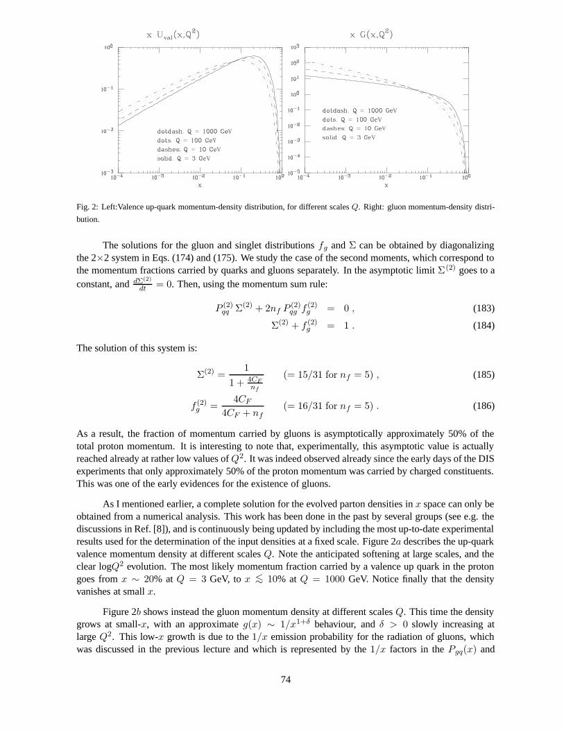
Fig. 2: Left:Valence up-quark momentum-density distribution, for different scales Q. Right: gluon momentum-density distri-

bution.

The solutions for the gluon and singlet distributions fg and Σ can be obtained by diagonalizingthe 2×2 system in Eqs. (174) and (175). We study the case of the second moments, which correspond tothe momentum fractions carried by quarks and gluons separately. In the asymptotic limit Σ(2) goes to aconstant, and dΣ(2)

dt = 0. Then, using the momentum sum rule:

P (2)qq Σ(2) + 2nf P

(2)qg f

(2)g = 0 , (183)

Σ(2) + f (2)g = 1 . (184)

The solution of this system is:

Σ(2) =1

1 + 4CFnf

(= 15/31 for nf = 5) , (185)

f (2)g =

4CF

4CF + nf(= 16/31 for nf = 5) . (186)

As a result, the fraction of momentum carried by gluons is asymptotically approximately 50% of thetotal proton momentum. It is interesting to note that, experimentally, this asymptotic value is actuallyreached already at rather low values ofQ2. It was indeed observed already since the early days of the DISexperiments that only approximately 50% of the proton momentum was carried by charged constituents.This was one of the early evidences for the existence of gluons.

As I mentioned earlier, a complete solution for the evolved parton densities in x space can only beobtained from a numerical analysis. This work has been done in the past by several groups (see e.g. thediscussions in Ref. [8]), and is continuously being updated by including the most up-to-date experimentalresults used for the determination of the input densities at a fixed scale. Figure 2a describes the up-quarkvalence momentum density at different scales Q. Note the anticipated softening at large scales, and theclear logQ2 evolution. The most likely momentum fraction carried by a valence up quark in the protongoes from x ∼ 20% at Q = 3 GeV, to x <∼ 10% at Q = 1000 GeV. Notice finally that the densityvanishes at small x.

Figure 2b shows instead the gluon momentum density at different scales Q. This time the densitygrows at small-x, with an approximate g(x) ∼ 1/x1+δ behaviour, and δ > 0 slowly increasing atlarge Q2. This low-x growth is due to the 1/x emission probability for the radiation of gluons, whichwas discussed in the previous lecture and which is represented by the 1/x factors in the Pgq(x) and

74

Fig. 3: Left: Sea up-quark momentum-density distribution, for different scales Q. Right: Momentum-density distribution for

several parton species, at Q = 1000 GeV.

Pgg(x) splitting functions. Figure 3a shows the up-quark sea momentum density at different scales Q.Shape and evolution match those of the gluon density, a consequence of the fact that sea quarks comefrom the splitting of gluons. Since the gluon-splitting probability is proportional to αs, the approximateratio sea/gluon ∼ 0.1 which can be obtained by comparing Figs. 2b and 3a is perfectly justified.

Finally, the momentum densities for gluons, up-sea, charm and up-valence distributions are shownin Fig. 3b for Q = 1000 GeV. Note here that usea and charm are approximately the same at very large Qand small x, The proton momentum is mostly carried by valence quarks and by gluons. The contributionof sea quarks is negligible.

6. QCD IN HADRONIC COLLISIONS

In hadronic collisions, all phenomena are QCD-related. The dynamics is more complex than in e+e−

or DIS, since both beam and target have a non-trivial partonic structure. As a result, calculations (andexperimental analyses) are more complicated. QCD phenomenology is however much richer, and thehigher energies available in hadronic collisions allow to probe the structure of the proton and of itsconstituents at the smallest scales attainable in a laboratory.

Contrary to the case of e+e− and lepton-hadron collisions, where calculations are routinely avail-able up to next-to-next-to-leading order (NNLO) accuracy, theoretical calculations for hadronic colli-sions are available at best with next-to-leading-order (NLO) accuracy. The only exception is the caseof Drell-Yan production, where NNLO results are known for the total cross sections. So we generallyhave relatively small precision in the theoretical predictions, and theoretical uncertainties which are largewhen compared to LEP or HERA.

However, pp collider physics is primarily discovery physics, rather than precision physics (thereare exceptions, such as the measurements of the W mass and of the properties of b-hadrons. But theseare not QCD-related measurements). As such, knowledge of QCD is essential both for the estimate ofthe expected signals, and for the evaluation of the backgrounds. Tests of QCD in pp collisions confirmour understanding of perturbation theory, or, when they fail, point to areas where our approximationsneed to be improved. (see, e.g., the theory advances prompted by the measurements of ψ production atCDF!).

75

Finally, a reliable theoretical control over the details of production dynamics allows one to extractimportant information on the structure of the proton (parton densities) in regions of Q2 and x otherwiseunaccessible. Control of QCD at the current machines (the Tevatron at Fermilab) is therefore essentialfor the extrapolation of predictions to higher energies (say for applications at the future LHC, at CERN).

The key ingredients for the calculation of production rates and distributions in hadronic colli-sions are:

• the matrix elements for the hard, partonic process (e.g., gg → gg, gg → bb, qq′ →W, . . .),

• the hadronic parton densities, discussed in the previous lecture.

Then the production rate for a given final state H is given by a factorization formula similar to the oneused to describe DIS:

dσ(pp→ H +X) =

∫

dx1 dx2

∑

i,j

fi(x1, Q) fj(x2.Q) dσ(ij → H) , (187)

where the parton densities fi’s are evaluated at a scale Q typical of the hard process under consideration.For example Q ' MDY for production of a Drell-Yan pair, Q ' ET for high transverse-energy (ET )jets, Q2 ' p2

T +m2Q for high-pT heavy quarks, etc.

In this lecture we will briefly explore two of the QCD phenomena currently studied in hadroniccollisions: Drell-Yan, and inclusive jet production. More details can be found in Refs. [8,4].

6.1. Drell-Yan processes

While the Z boson has been recently studied with great precision by the LEP experiments, it was actuallydiscovered, together with the W boson, by the CERN experiments UA1 and UA2 in pp collisions. Wphysics is now being studied in great detail at LEP2, but the best direct measurements of its mass bya single group still belong to pp experiments (CDF and D0 at the Tevatron). Even after the ultimateluminosity will have been accumulated at LEP2, with a great improvement in the determination of theparameters of the W boson, the monopoly of W studies will immediately return to hadron colliders, withthe Tevatron data-taking resuming in the year 2000, and later on with the start of the LHC experiments.

Precision measurements of W production in hadronic collisions are important for several reasons:

• this is the only process in hadronic collisions which is known to NNLO accuracy

• the rapidity distribution of the charged leptons from W decays is sensitive to the ratio of the upand down quark densities, and can contribute to our understanding of the proton structure.

• deviations from the expected production rates of highly virtual W ’s (pp → W ∗ → eν) are apossible signal of the existence of new W bosons, and therefore of new gauge interactions.

The partonic cross-section for the production of a W boson from the annihilation of a qq pair canbe easily calculated, giving the following result [8,4]:

σ(qiqj → W ) = π

√2

3|Vij |2 GF M2

W δ(s−M 2W ) = Aij M

2W δ(s−M 2

W ) , (188)

where s is partonic center of mass energy squared, and Vij is the element of the Cabibbo-Kobayashi-Maskawa matrix. The delta function comes from the 2 → 1 phase space, which forces the center-of-massenergy of the initial state to coincide with the W mass. It is useful to introduce the two variables

τ =s

Shad≡ x1x2 , (189)

76

y =1

2log

(

EW + pzW

EW − pzW

)

≡ 1

2log

(x1

x2

)

, (190)

where Shad is the hadronic center of mass energy squared. The variable y is called rapidity. For slowlymoving objects it reduces to the standard velocity, but, contrary to the velocity, it transforms additivelyeven at high energies under Lorentz boosts along the direction of motion. Written in terms of τ andy, the integration measure over the initial-state parton momenta becomes: dx1dx2 = dτdy. Using thisexpression and Eq. (188) in Eq. (187), we obtain the following result for the LO total W production crosssection:

σDY =∑

i,j

π Aij

M2W

τ

∫ 1

τ

dx

xfi(x) fj

(τ

x

)

≡∑

i,j

π Aij

M2W

τLij(τ) , (191)

where the function Lij(τ) is usually called partonic luminosity. In the case of ud collisions, the overallfactor in front of this expression has a value of approximately 6.5 nb. It is interesting to study the partonicluminosity as a function of the hadronic CoM energy. This can be done by taking a simple approximationfor the parton densities. Following the indications of the figures presented in the previous lecture, weshall assume that fi(x) ∼ 1/x1+δ , with δ < 1. Then

L(τ) =

∫ 1

τ

dx

x

1

x1+δ

(x

τ

)1+δ

=1

τ1+δ

∫ 1

τ

dx

x=

1

τ1+δlog

(1

τ

)

(192)

and

σW ∼ τ−δ log

(1

τ

)

=

(

Shad

M2W

)δ

log

(

Shad

M2W

)

. (193)

The DY cross-section grows therefore at least logarithmically with the hadronic CM energy. This is tobe compared with the behaviour of the Z production cross section in e+e− collisions, which is steeplydiminuishing for values of s well above the production threshold. The reason for the different behaviourin hadronic collisions is that while the energy of the hadronic initial state grows, it will always be possibleto find partons inside the hadrons with the appropriate energy to produce the W directly on-shell. Thenumber of partons available for the production of a W is furthermore increasing with the increase inhadronic energy, since the larger the hadron energy, the smaller will be the value of hadron momentumfraction x necessary to produce theW . The increasing number of partons available at smaller and smallervalues of x causes then the growth of the total W production cross section.

A comparison between the best available prediction for the production rates of W and Z bosonsin hadronic collisions, and the experimental data, is shown in Fig. 4. The experimental uncertainties willsoon be dominated by the limited knowledge of the machine luminosity, and will exceed the accuracyof the NNLO predictions. This suggests that in the future the total rate of produced W bosons could beused as an accurate luminometer.

It is also interesting to note that an accurate measurement of the relative W and Z production rates(which is not affected by the knowledge of the total integrated luminosity, that will cancel in their ratio)provides a tool to measure the total W width. This can be seen from the following equation:

ΓW =Nobs(Z → e+e−)

Nobs(W → e±ν)

(σW±

σZ

) (

ΓWeν

ΓZe+e−

)

ΓZ .

↑ ↑measure calculable LEP/SLC

As of today, this technique provides the best measurement of ΓW : ΓW = 2.06 ± 0.06 GeV, which is afactor of 5 more accurate than the current best direct measurements from LEP2.

77

0.4

0.50.60.70.80.9

1

2

3

4

0.4 0.6 0.8 1 1.2 1.4 1.6 1.8 2 2.2 2.4

CDF eD0 eD0 µUA1 µUA2 e

σB(W

→lν

) (n

b)

(a)

2.3

2.4

2.5

2.6

2.7

0 2.5 5 7.5 10

1 2 3 4 5PDF Set

0.04

0.050.060.070.080.090.1

0.2

0.3

0.4 0.6 0.8 1 1.2 1.4 1.6 1.8 2 2.2 2.4Center of Mass Energy (TeV)

σB(Z

0 →l+

l- ) (n

b)

(b)

0.21

0.22

0.23

0.24

0.25

0 2.5 5 7.5 10

1 2 3 4 5PDF Set

Fig. 4: Comparison of measured (a) σ ·B(W → eν) and (b) σ ·B(Z0 → e+e−) to 2-loop theoretical predictions using MRSA

parton distribution functions. The UA1 and UA2 measurements and D0 measurements are offset horizontally by ± 0.02 TeV

for clarity. In the inset, the shaded area shows the 1σ region of the CDF measurement; the stars show the predictions using

various parton distribution function sets (1) MRSA, (2) MRSD0′, (3)MRSD-′, (4) MRSH and (5) CTEQ2M. The theoretical

points include a common uncertainty in the predictions from choice of renormalization scale (MW /2 to 2MW ).

6.2. W rapidity asymmetry

The measurement of the charge asymmetry in the rapidity distribution of W bosons produced in ppcollisions can provide an important measurement of the ratio of the u-quark and d-quark momentumdistributions. Using the formulas provided above, you can in fact easily check as an exercise that:

dσW+

dy∝ fp

u(x1) fpd(x2) + fp

d(x1)f

pu(x2) , (194)

dσW−

dy∝ fp

u(x1) fpd (x2) + fp

d (x1)fpu(x2) . (195)

We can then construct the following charge asymmetry (assuming the dominance of the quark densitiesover the antiquark ones, which is valid in the kinematical region of interest for W production at theTevatron):

A(y) =

dσW+

dy − dσW−dy

dσW+

dy +dσW−

dy

=fp

u(x1) fpd (x2) − fp

d (x1) fpu(x2)

fpu(x1) f

pd (x2) + fp

d (x1) fpu(x2)

. (196)

78

Setting fd(x) = fu(x) R(x) we then get:

A(y) =R(x2) −R(x1)

R(x2) +R(x1), (197)

which measures the R(x) ratio since x1,2 are known in principle from the kinematics: x1,2 =√τ exp(±y)4. The current CDF data provide the most accurate measurement to date of this quantity

(see Ref. [8]).

6.3. Jet production

Jet production is the hard process with the largest rate in hadronic collisions. For example, the crosssection for producing at the Tevatron (

√Shad = 1.8 TeV) jets of transverse energy Ejet

T<∼ 50 GeV is

of the order of a µb. This means 50 events/sec at the luminosities available at the Tevatron. The datacollected at the Tevatron so far extend all the way up to the ET values of the order of 450 GeV. Theseevents are generated by collisions among partons which carry over 50% of the available pp energy, andallow to probe the shortest distances ever reached. The leading mechanisms for jet production are shownin Fig. 5.

Fig. 5: Representative diagrams for the production of jet pairs in hadronic collisions.

The 2-jet inclusive cross section can be obtained from the formula

dσ =∑

ijkl

dx1 dx2 f(H1)i (x1, µ) f

(H2)j (x2, µ)

dσij→k+l

dΦ2dΦ2 , (198)

that has to be expressed in terms of the rapidity and transverse momentum of the quarks (or jets), in orderto make contact with physical reality. The two-particle phase space is given by

dΦ2 =d3k

2k0(2π)32π δ((p1 + p2 − k)2) , (199)

and, in the CM of the colliding partons, we get

dΦ2 =1

2(2π)2d2kT dy 2 δ(s − 4(k0)2 ) , (200)

where kT is the transverse momentum of the final-state partons. Here y is the rapidity of the produced4In practice one cannot determine x1,2 with arbitrary precision on an event-by-event basis, since the longitudinal momentum

of the neutrino cannot be easily measured. The actual measurement is therefore done by studying the charge asymmetry in therapidity distribution of the charged lepton.

79

parton in the parton CM frame. It is given by

y =y1 − y2

2, (201)

where y1 and y2 are the rapidities of the produced partons in the laboratory frame (in fact, in any frame).One also introduces

y0 =y1 + y2

2=

1

2log

x1

x2, τ =

s

Shad= x1 x2 . (202)

We havedx1 dx2 = dy0 dτ . (203)

We obtain

dσ =∑

ijkl

dy01

Shadf

(H1)i (x1, µ) f

(H2)j (x2, µ)

dσij→k+l

dΦ2

1

2(2π)22 dy d2kT , (204)

which can also be written as

dσ

dy1 dy2 d2kT=

1

Shad 2(2π)2

∑

ijkl

f(H1)i (x1, µ) f

(H2)j (x2, µ)

dσij→k+l

dΦ2. (205)

The variables x1, x2 can be obtained from y1, y2 and kT from the equations

y0 =y1 + y2

2, (206)

y =y1 − y2

2, (207)

xT =2kT√Shad

, (208)

x1 = xT ey0 cosh y , (209)

x2 = xT e−y0 cosh y . (210)

For the partonic variables, we need s and the scattering angle in the parton CM frame θ, since

t = − s2

(1 − cos θ) , u = − s2

(1 + cos θ) . (211)

Neglecting the parton masses, you can show that the rapidity can also be written as:

y = − log tanθ

2≡ η , (212)

with η being usually referred to as pseudorapidity.The leading-order Born cross sections for parton parton scattering are reported in Table 1. It is

interesting to note that a good approximation to the exact results can be easily obtained by using the soft-gluon techniques introduced in the third lecture. Based on the fact that even at 90 min(|t|, |u|) does notexceed s/2, and that therefore everything else being equal a propagator in the t or u channel contributesto the square of an amplitude 4 times more than a propagator in the s channel, it is reasonable to assumethat the amplitudes are dominated by the diagrams with a gluon exchanged in the t (or u) channel. Itis easy to calculate the amplitudes in this limit using the soft-gluon approximation. For example, theamplitude for the exchange of a soft gluon among a qq ′ pair is given by:

(λaij) (λa

kl) 2pµ1

t2p′µ = λa

ij λakl

4p · p′t

=2s

tλa

ij λakl . (213)

80

Process dσdΦ2

qq′ → qq′ 12s

49

s2+u2

t2

qq → qq 12

12s

[49

(s2+u2

t2+ s2+t2

u2

)

− 827

s2

ut

]

qq → q′q′ 12s

49

t2+u2

s2

qq → qq 12s

[49

(s2+u2

t2+ t2+u2

s2

)

− 827

u2

st

]

qq → gg 12

12s

[3227

t2+u2

tu− 8

3t2+u2

s2

]

gg → qq 12s

[16

t2+u2

tu− 3

8t2+u2

s2

]

gq → gq 12s

[

−49

s2+u2

su + u2+s2

t2

]

gg → gg 12

12s

92

(

3 − tus2 − su

t2− st

u2

)

Table 1: Cross sections for light parton scattering. The notation is p1 p2 → k l, s = (p1 + p2)2, t = (p1 − k)2, u = (p1 − l)2.

The pµ and p′µ factors represent the coupling of the exchanged gluon to the q and q ′ quark lines, respec-tively (see Eq. (105). Squaring, and summing and averaging over spins and colours, gives

∑

colours,spin

|Mqq′ |2 =1

N2

(

N2 − 1

4

)

4s2

t2=

8

9

s2

t2. (214)

Since for this process the diagram with a t-channel gluon exchange is symmetric for s ↔ u exchange,and since u → −s in the t → 0 limit, the above result can be rewritten in an explicitly (s, u) symmetricway as

4

9

s2 + u2

t2, (215)

which indeed exactly agrees with the result of the exact calculation, as given in Table 1. The correctionswhich appear from s or u gluon exchange when the quark flavours are the same or when we study a qqprocess are small, as can be seen by comparing the above result to the expressions in the Table.

As another example we consider the case of qg → qg scattering. The amplitude will be exactlythe same as in the qq′ → qq′ case, up to the different colour factors. A simple calculation then gives:

∑

colours,spin

|Mqg|2 =9

4

∑

|Mqq′ |2 =s2 + u2

t2. (216)

The exact result isu2 + s2

t2− 4

9

u2 + s2

us, (217)

which even at 90, the point where the t-channel exchange approximation is worse, only differs fromthis latter by no more than 25%.

As a final example we consider the case of gg → gg scattering, which in our approximation gives:

∑

|Mgg|2 =9

2

s2

t2. (218)

By u↔ t symmetry we should expect the simple improvement:

∑

|Mgg|2 ∼ 9

2

(

s2

t2+s2

u2

)

. (219)

81

This only differs by 20% from the exact result at 90.

Notice that at small t the following relation holds:

σgg : σqg : σqq =

(9

4

)

: 1 :

(4

9

)

. (220)

The 9/4 factors are simply the ratios of the colour factors for the coupling to gluons of a gluon (CA)and of a quark (TF ), after including the respective colour-average factors (1/(N 2 − 1) for the gluon, and1/N for the quark). Using Eq. (220), we can then write:

dσhadr =

∫

dx1 dx2

∑

i,j

fi(x1) fj(x2) dσij =

∫

dx1 dx2 F (x1) F (x2) dσgg(gg → jets) , (221)

where the object:

F (x) = fg(x) +4

9

∑

f

[qf (x) + qf (x)] (222)

is usually called the effective structure function. This result indicates that the measurement of the inclu-sive jet cross section does not allow in principle to disentangle the independent contribution of the variouspartonic components of the proton, unless of course one is considering a kinematical region where theproduction is dominated by a single process. The relative contributions of the different channels, aspredicted using the global fits of parton densities available in the literature, are shown in Fig. 6.

Fig. 6: Relative contribution to the inclusive jet-ET rates from the different production channels.

Predictions for jet production at colliders are available today at the next-to-leading order in QCD.A comparison between these calculations and the available data is given in Figs. 7 and 8.

At the Tevatron, jets up to 450 GeV transverse momentum have been observed. That is x >∼ 0.5and Q2 ' 160, 000 GeV2. This is a domain of x and Q2 not accessible to HERA. The current agreementbetween theory and data is at the level of 30 % over 8 orders of magnitude of cross-section, from ET ∼20 to ET ∼ 450 GeV. The small deviation observed by CDF at high ET is under active investigationboth experimentally and theoretically. It is still premature to say whether it can be a signal of newphenomena, or whether it is the result of our incomplete knowledge of the gluon density at large x.Either way, future higher-statistics measurements at the Tevatron will provide some important input onthese fundamental questions. The resulting knowledge will enable theorists to reliably predict productionrates for all interesting processes that will take place at the LHC.

82

1/∆η

∫d2 σ/

(dE

Tdη

) f

b/G

eV

CTEQ3M µ=ET(max)/2

Unsmeared Data

Jet ET (GeV)

Sys.

Err

or (

%)

10-1

1

10

10 2

10 3

10 4

10 5

10 6

10 7

-50%

0%

50%

50 100 150 200 250 300 350 400 450 500

Fig. 7: Inclusive ET spectra for central jets at the Tevatron

Jet ET (GeV)

(Dat

a-T

heor

y)/T

heor

y

(94-95) Data 93 pb-1

-1.5

-1

-0.5

0

0.5

1

1.5

50 100 150 200 250 300 350 400 450 500

Transverse Energy

(DATA-THEORY)/THEORY

-100

-75

-50

-25

0

25

50

75

100

125

150

0 50 100 150 200 250 300 350 400 450

(GeV)

Per

cent

age

CDF Preliminary

Run 1B (87 pb-1)with run 1A results overlayed

NLO QCD CTEQ3M scale Et/2

Statistical errors only

Fig. 8: Comparison of inclusive jets cross sections with QCD calculations at the Tevatron.

ACKNOWLEDGEMENT

It is a pleasure to thank the organizers of this School, for the successful efforts made to bring top-quality students together, and to provide a great environment for physics discussions and for a pleasanttime as well.

83

References

Standard Textbooks:

[1] R.P. Feynman, Photon-Hadron Interactions, W.A. Benjamin, NY (1972).

[2] B.L. Ioffe, V.A. Khoze and L.N. Lipatov, Hard Processes, North Holland (1984).

[3] T. Muta, Foundations of QCD, World Scientific (1987).

[4] V. Barger and R.J.N. Phillips, Collider Physics, Addison Wesley (1987).

[5] R. Field, Applications of Perturbative QCD, Addison Wesley (1989).

[6] Yu.L. Dokshitzer, V.A. Khoze, A.H. Mueller and S.I. Troyan, Basics of Perturbative QCD,Editions Frontieres (1991).

[7] M.E. Peskin and D.V. Schroeder: An Introduction to Quantum Field Theory, Addison-Wesley (1995).

[8] R.K. Ellis, W.J. Stirling and B.R. Webber: QCD and Collider Physics, Cambridge UniversityPress (1996).

Pedagogical Reviews

[9] P. Nason, lectures delivered at the 1997 CERN School.

[10] Yu.L. Dokshitzer, lectures delivered at the 1995 CERN School.

[11] M. Neubert, lectures delivered at the 1994 CERN School.

Review Articles

[12] G. Altarelli, Phys. Rep. 81 (1982) 1.

[13] A.H. Mueller, Phys. Rev. 73 (1981) 237.

[14] Yu.L. Dokshitzer, D.I. Dyakonov and S.I. Trojan, Phys. Rep. 58 (1980) 270.

[15] A. Bassetto, M. Ciafaloni and G. Marchesini, Phys. Rep. 100 (1983) 201.

[16] M.L. Mangano and S.J. Parke, Phys. Rep. 200 (1991) 301.

Historical Reviews

[17] D.J. Gross, hep-th/9809060.

[18] G. ’t Hooft, hep-th/9808154.

84