Introduction to Predictive Models Book Chapters 1, 2 and 5. · 1. Introduction to Predictive Models...
67
Introduction to Predictive Models Book Chapters 1, 2 and 5. Carlos M. Carvalho The University of Texas McCombs School of Business 1
Transcript of Introduction to Predictive Models Book Chapters 1, 2 and 5. · 1. Introduction to Predictive Models...

Introduction to Predictive ModelsBook Chapters 1, 2 and 5.
Carlos M. CarvalhoThe University of Texas McCombs School of Business
1

1. Introduction
2. Measuring Accuracy
3. Out-of Sample Predictions
4. Bias-Variance Trade-Off
5. Classification
6. Cross-Validation
7. k-Nearest Neighbors (kNN)

1. Introduction to Predictive Models
Simply put, the goal is to predict a
target variable Y with input variables X !
In Data Mining terminology this is know as supervised learning
(also called Predictive Analytics).
In general, a useful way to think about it is that Y and X are
related in the following way:
Yi = f (Xi ) + εi
The main purpose of this part of the course is to learn or estimate
f (·) from data1
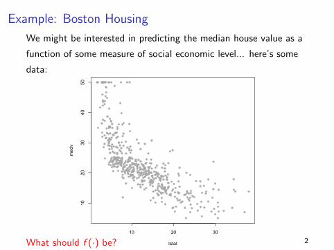
Example: Boston Housing
We might be interested in predicting the median house value as a
function of some measure of social economic level... here’s some
data:
10 20 30
1020
3040
50
lstat
medv
What should f (·) be? 2

Example: Boston Housing
How about this...
10 20 30
1020
3040
50
lstat
medv
If lstat = 30 what is the prediction for medv? 3

Example: Boston Housing
or this...
10 20 30
1020
3040
50
lstat
medv
If lstat = 30 what is the prediction for medv? 4

Example: Boston Housing
or even this?
10 20 30
1020
3040
50
lstat
medv
If lstat = 30 what is the prediction for medv? 5
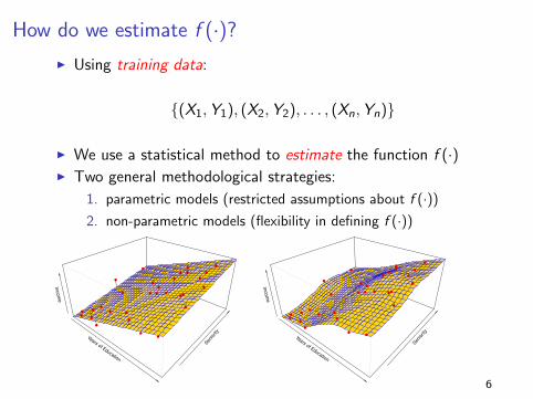
How do we estimate f (·)?
I Using training data:
{(X1,Y1), (X2,Y2), . . . , (Xn,Yn)}
I We use a statistical method to estimate the function f (·)I Two general methodological strategies:
1. parametric models (restricted assumptions about f (·))
2. non-parametric models (flexibility in defining f (·))
Years of Education
Sen
iorit
y
Incom
e
Years of Education
Sen
iorit
y
Incom
e
6

Back to Boston Housing
Parametric Model Non-Parametric Model
(Y = µ+ ε) (k-nearest neighbors)
10 20 30
1020
3040
50
lstat
medv
10 20 30
1020
3040
50
lstat
medv
7
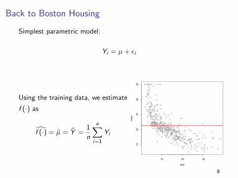
Back to Boston Housing
Simplest parametric model:
Yi = µ+ εi
Using the training data, we estimate
f (·) as
f (·) = µ = Y =1
n
n∑i=1
Yi
10 20 30
1020
3040
50
lstat
medv
8

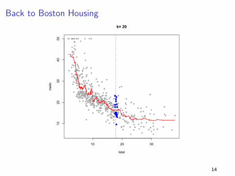
Back to Boston Housing
The above strategy averages all points in the training set... maybe
points that are “closer” to the place I am trying to predict should
be more relevant...
How about averaging the closest 20 neighbors?
What do I mean by closest? We will choose the 20 points that are
closest to the X value we are trying to predict.
This is what is called the k-nearest neighbors algorithm
9

Back to Boston Housing
10 20 30
1020
3040
50
k= 20
lstat
medv
10

Back to Boston Housing
10 20 30
1020
3040
50
k= 20
lstat
medv
11

Back to Boston Housing
10 20 30
1020
3040
50
k= 20
lstat
medv
12

Back to Boston Housing
10 20 30
1020
3040
50
k= 20
lstat
medv
13
Back to Boston Housing
10 20 30
1020
3040
50
k= 20
lstat
medv
14

Back to Boston Housing
10 20 30
1020
3040
50
k= 20
lstat
medv
15

Back to Boston Housing
Okay, that seems sensible but why not use 2 neighbors or 200
neighbors?
10 20 30
1020
3040
50
k= 2
lstat
medv
16

Back to Boston Housing
Okay, that seems sensible but why not use 5 neighbors or 200
neighbors?
10 20 30
1020
3040
50
k= 10
lstat
medv
17

Back to Boston Housing
Okay, that seems sensible but why not use 5 neighbors or 200
neighbors?
10 20 30
1020
3040
50
k= 50
lstat
medv
18

Back to Boston Housing
Okay, that seems sensible but why not use 5 neighbors or 200
neighbors?
10 20 30
1020
3040
50
k= 100
lstat
medv
19

Back to Boston Housing
Okay, that seems sensible but why not use 5 neighbors or 200
neighbors?
10 20 30
1020
3040
50
k= 150
lstat
medv
20
Back to Boston Housing
Okay, that seems sensible but why not use 5 neighbors or 200
neighbors?
10 20 30
1020
3040
50
k= 200
lstat
medv
21

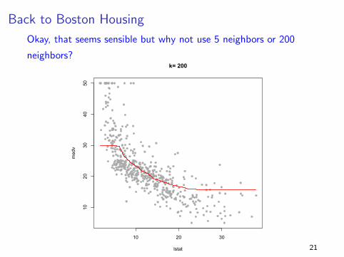
Back to Boston Housing
Okay, that seems sensible but why not use 5 neighbors or 200
neighbors?
10 20 30
1020
3040
50
k= 400
lstat
medv
22

Back to Boston Housing
Okay, that seems sensible but why not use 5 neighbors or 200
neighbors?
10 20 30
1020
3040
50
k= 505
lstat
medv
23

Complexity, Generalization and Interpretation
I As we have seen in the examples above, there are lots of
options in estimating f (X ).I Some methods are very flexible some are not... why would we
ever choose a less flexible model?
1. Simple, more restrictive methods are usually easier to interpret
2. More importantly, it is often the case that simpler models are
more accurate in making future predictions.
Not too simple, but not too complex!
10 20 30
1020
3040
50
lstat
medv
10 20 30
1020
3040
50
k= 150
lstat
medv
10 20 30
1020
3040
50
k= 2
lstatmedv
24

2. Measuring Accuracy
How accurate are each of these models?
Using the training data a standard measure of accuracy is the root
mean-squared error
RMSE =
√√√√1
n
n∑i=1
[Yi − f (Xi )
]2
This measure, on average, how large the “mistakes” (errors) made
by the model are...
25

Measuring Accuracy (Boston housing, again)
10 20 30
1020
3040
50
k= 505
lstat
medv
10 20 30
1020
3040
50
k= 150
lstat
medv
10 20 30
1020
3040
50
k= 2
lstat
medv
-6 -5 -4 -3 -2 -1
45
67
89
Complexity (log(1/k))
RMSE
k= 2
k= 505
k= 150
So, I guess we should just go
with the most complex model,
i.e., k = 2, right?
26

3. Out-of Sample Predictions
But, do we really care about explaining what we have already seen?
Key Idea: what really matters is our prediction accuracy
out-of-sample!!!
Suppose we have m additional observations (X oi ,Y
oi ), for
i = 1, . . . ,m, that we did not use to fit the model. Let’s call this
dataset the validation set (also known as hold-out set or test set)
Let’s look at the out-of-sample RMSE:
RMSE o =
√√√√ 1
m
m∑i=1
[Y oi − f (X o
i )]2
27

Out-of Sample Predictions
In our Boston housing example, I randomly chose a training set of
size 400. I re-estimate the models using only this set and use the
models to predict the remaining 106 observations (validation set)...
-6 -5 -4 -3 -2 -1
5.0
5.5
6.0
6.5
7.0
7.5
8.0
Complexity (log(1/k))
out-o
f-sam
ple
RM
SE
k= 46
k= 2
k= 345
Now, the model where
k = 46 looks like the
most accurate choice!!
Not too simple but not
too complex!!!
28

The Key Idea of the Course!!
Elements of Statistical Learning (2nd Ed.) c!Hastie, Tibshirani & Friedman 2009 Chap 2
High BiasLow Variance
Low BiasHigh Variance
Pre
dic
tion
Err
or
Model Complexity
Training Sample
Test Sample
Low High
FIGURE 2.11. Test and training error as a functionof model complexity.
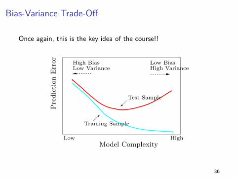
This shows the typical behavior of the in and out-of-sample
prediction error as a function of the complexity of the model... too
flexible models will adapt itself too closely to the the training set
and will not generalize well, i.e., not be very good for the test data.29

4. Bias-Variance Trade-Off
Why do complex models behave poorly in making predictions?
Let’s start with an example...
I In the Boston housing example, I will randomly choose 30
observations to be in the training set 3 different times...
I for each training set I will estimate f (·) using the k-nearest
neighbors idea... first with k = 2 and them with k = 20
30

Bias-Variance Trade-Off
k=2 Hi variability...
10 20 30
1020
3040
50
k= 2
lstat
medv
10 20 30
1020
3040
50
k= 2
lstat
medv
10 20 30
1020
3040
50
k= 2
lstat
medv
(blue points are the training data used)31

Bias-Variance Trade-Off
k=20 Low variability ... but BIAS!!
10 20 30
1020
3040
50
k= 20
lstat
medv
10 20 30
1020
3040
50
k= 20
lstat
medv
10 20 30
1020
3040
50
k= 20
lstat
medv
(blue points are the training data used)32

Bias-Variance Trade-Off
What did we see here?
I When k = 2, it seems that the estimate of f (·) varies a lot
between training sets...
I When k = 20 the estimates look a lot more stable...
Now, imagine that you are trying to predict medv when
lstat = 20... compare the changes in the predictions made by the
different training sets under k = 2 and k = 20... what do you see?
33

Bias-Variance Trade-Off
I This is an illustration of what is called the bias-variance
trade-off.
I In general, simple models are trying to explain a complex, real
problem with not a lot of flexibility so it introduces bias... on
the other hand, by being simple the estimates tend to have
low variance
I On the other hand, complex models are able to quickly adapt
to the real situation and hence lead to small bias... however,
by being to adaptable, it tends to vary a lot, i.e., high
variance.
34
Bias-Variance Trade-Off
I In other words, we are trying to capture important patterns of
the data that generalize to the future observations we are
trying to predict. Models that are too simple are not able to
capture relevant patterns and might have too big of a bias in
predictions...
I Models that are too complex will “chase” irrelevant patterns
in the training data that are not likely to exist in future data...
so, it will lead to predictions that will vary a lot as things could
change a lot depending on what sample we happen to see.
I Our goal is to find the sweet spot in the bias-variance
trade-off!!
35
Bias-Variance Trade-Off
Once again, this is the key idea of the course!!
Elements of Statistical Learning (2nd Ed.) c!Hastie, Tibshirani & Friedman 2009 Chap 2
High BiasLow Variance
Low BiasHigh Variance
Pre
dic
tion
Err
or
Model Complexity
Training Sample
Test Sample
Low High
FIGURE 2.11. Test and training error as a functionof model complexity. 36

Bias-Variance Trade-Off
Let’s get back to our original representation of the problem... it
helps us understand what is going on...
Yf = f (Xf ) + ε
I We need flexible enough models to find f (·) without imposing
bias...
I ... but, too flexible models will “chase” non-existing patterns
in ε leading to unwanted variability
37

Bias-Variance Trade-Off
A more detailed look at this idea... assume we are trying to make
a prediction for Yf using Xf and our inferred f (·). We hope to
make small mistake measured by squared distance... Let’s explore
how our mistakes will behave on average.
E[(Yf − f (Xf ))2
]=
(f (Xf )− E
[f (Xf )
])2+ Var
[f (Xf )
]+ Var(ε)
= Bias[f (Xf )
]2+ Var
[f (Xf )
]+ Var(ε)
hence, the Bias-Variance Trade-Off!!
38

5. Classification
Classification is the term used when we want to predict a Y that is
a category... win/lose, sick/healthy, pay/default, good/bad...
below is an example where we are trying to predict whether or not
the favorite team will win as a function of the Vegas’ betting
point-spread.
spread
Frequency
0 10 20 30 40
020
4060
80100
120 favwin=1favwin=0
01
0 10 20 30 40
spread
favwin
39

Classification
In this context, f (X ) will output the probability of Y taking a
particular category (win/lose,here). Below, the black line represent
different methods to estimate f (X ) in this example.
0 10 20 30 40
0.0
0.2
0.4
0.6
0.8
1.0
linear regression
spread
favwin
0 10 20 30 40
0.0
0.2
0.4
0.6
0.8
1.0
logistic regression
spread
favwin
0 10 20 30 40
0.0
0.2
0.4
0.6
0.8
1.0
knn(5)
spread
favwin
0 10 20 30 40
0.0
0.2
0.4
0.6
0.8
1.0
knn(20)
spread
favwin
40

Classification
All the discussion about complexity vs. predictive accuracy
(bias-variance trade-off) applies to this setting... what differs is our
measure of accuracy as we are no longer dealing with a numerical
outcome variable. A common approach is to measure the error
rate, i.e., the number of times we a estimated f (·) “gets it
wrong”... in the training set (with n observations) define the error
rate as:1
n
n∑i=1
I(Yi 6= Yi )
where Yi is the class (category) label assigned by f (Xi ) and I(·) is
an indicator variable that equals 1 whenever Yi 6= Yi and 0
otherwise.
41
Classification
As mentioned above, in classification, f (Xi ) outputs a probability.
In order to use this information and create a classification rule we
need to decide on a cut-off (or cut-offs) to determined the label
assignments.
In general, if we are looking at only two categories (like the NBA
example above) the standard cut-off is 0.5. This means that if
f (Xf ) > 0.5 we define Yi = 1 (Yi = 0 otherwise).
Later on, we will think more carefully about defining cut-offs...
42
Classification
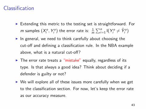
I Extending this metric to the testing set is straightforward. For
m samples (X oi ,Y
oi ) the error rate is: 1
m
∑ni=1 I(Y o
i 6= Y oi )
I In general, we need to think carefully about choosing the
cut-off and defining a classification rule. In the NBA example
above, what is a natural cut-off?
I The error rate treats a “mistake” equally, regardless of its
type. Is that always a good idea? Think about deciding if a
defender is guilty or not?
I We will explore all of these issues more carefully when we get
to the classification section. For now, let’s keep the error rate
as our accuracy measure.
43
6. Cross-Validation
I Using a validation-set to evaluate the performance of
competing models has two potential drawbacks:
1. the results can be highly dependent on the choice of the
validation set... what samples? how many?
2. by leaving aside a subset of data for validation we end up
estimating the models with less information. It is harder to
learn with fewer samples and this might lead to an
overestimation of errors.
I Cross-Validation is a refinement of the validation strategy that
help address both of these issues.
44

Leave-One-Out Cross-Validation (loocv)
The name says it all!
I Assume we have n samples in our dataset. Define the
validation set by choosing only one sample. Call it the i th
observation...
I The model is then trained in the remaining n − 1 samples and
the results are used to predict the left-out sample. Compute
the squared-error MSEi = (Yi − Yi )2
I Repeat the procedure for every sample in the dataset (n
times) and compute the average cross-validation MSE:
MSE loocv =1
n
n∑i=1
MSEi
45
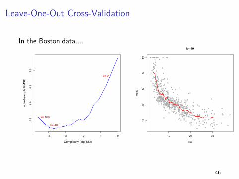
Leave-One-Out Cross-Validation
In the Boston data....
-4 -3 -2 -1 0
5.5
6.0
6.5
7.0
Complexity (log(1/k))
out-o
f-sam
ple
RM
SE
k= 40
k= 2
k= 100
10 20 30
1020
3040
50
k= 40
lstat
medv
46

k-fold Cross Validation
LOOCV can be computationally expensive as each model being
considered has to be estimated n times! A popular alternative is
what is called k-fold Cross Validation.
I This approach randomly divides the original dataset into k
groups of approximately the same size
I Choose one of the groups as a validation set. Estimate the
models with the remaining k − 1 groups and predict the
samples in the validation set. Compute the average
squared-error for the samples in the validation set
MSEi = Average[(Yi − Yi )
2]
I Repeat the procedure for every fold in the dataset (k times)
and compute the average cross-validation MSE:
MSE kcv = 1k
∑ki=1 MSEi 47

k-fold Cross Validation
The usual choices are between k = 5 and k = 10...
-4 -3 -2 -1 0
5.5
6.0
6.5
7.0
kfold( 5 )
Complexity (log(1/k))
out-o
f-sam
ple
RM
SE
k= 29
k= 2
k= 100
-4 -3 -2 -1 0
5.5
6.0
6.5
7.0
7.5
kfold( 10 )
Complexity (log(1/k))
out-o
f-sam
ple
RM
SE
k= 37
k= 2
k= 100
48

k-fold Cross Validation
I Bias-Variance Trade-Off: LOOCV has a smaller bias as it uses
more information in the training sets... but it also has more
variance! By only leaving a sample out at a time, the training
set doesn’t change much so the outputs will be very correlated
with each other. So, the resulting MSE will be a average off
correlated quantities which tends to be more variable
I In k-fold the outputs are not very correlated as the training
sets can be quite different and the resulting MSE is an average
of somewhat “independent” quantities... hence less variance!
I There is a bias-variance trade-off between LOOCV and k-fold.
The choice of k = 5 or k = 10 has been empirically shown to
be a good choice that neither suffers from a lot of bias nor
from a lot of variance! 49

7. k-Nearest Neighbors (kNN)
The k-nearest neighbors algorithm will try to predict (numerical
variables) or classify (categorical variables) based on similar (close)
records on the training dataset.
Remember, the problem is to guess a future value Yf given new
values of the covariates Xf = (x1f , x2f , x3f , . . . , xpf ).
50

k-Nearest Neighbors (kNN)
kNN: How do the Y ′s look like close to the region around
Xf ?
We need to find the k records in the training dataset that are close
to Xf . How? “Nearness” to the i th neighbor can be defined by
(euclidian distance):
di =
√√√√ p∑j=1
(xjf − xji )2
Prediction:
I Numerical Yf : take the average of the Y ′s in the k-nearest
neighbors
I Categorical Yf : take the most common category in the
k-nearest neighbors 51

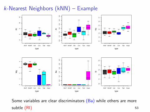
k-Nearest Neighbors (kNN) – Example
Forensic Glass Analysis
Classifying shards of glass
Refractive index, plus oxide %
Na, Mg, Al, Si, K, Ca, Ba, Fe.
6 possible glass types
WinF: float glass window
WinNF: non-float window
Veh: vehicle window
Con: container (bottles)
Tabl: tableware
Head: vehicle headlamp
3
52
k-Nearest Neighbors (kNN) – Example
WinF WinNF Veh Con Tabl Head
-50
510
15
type
RI
WinF WinNF Veh Con Tabl Head
0.5
1.0
1.5
2.0
2.5
3.0
3.5
type
Al
WinF WinNF Veh Con Tabl Head
1112
1314
1516
17
type
Na
WinF WinNF Veh Con Tabl Head
01
23
4
type
Mg
WinF WinNF Veh Con Tabl Head
0.0
0.5
1.0
1.5
2.0
2.5
3.0
type
Ba
WinF WinNF Veh Con Tabl Head
7071
7273
7475
type
Si
Some variables are clear discriminators (Ba) while others are more
subtle (RI) 53

k-Nearest Neighbors (kNN) – Example
Using only RI and AI let’s try to predict the point marked by “?”
-2 -1 0 1 2 3 4
-20
24
1-nearest neighbor
Al
RI
?
54

k-Nearest Neighbors (kNN) – Example
-2 -1 0 1 2 3 4
-20
24
1-nearest neighbor
Al
RI
55

k-Nearest Neighbors (kNN) – Example
-2 -1 0 1 2 3 4
-20
24
5-nearest neighbor
Al
RI
?
56
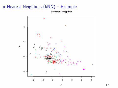
k-Nearest Neighbors (kNN) – Example
-2 -1 0 1 2 3 4
-20
24
5-nearest neighbor
Al
RI
57

k-Nearest Neighbors (kNN)
Comments:
I kNN is simple and intuitive and yet very powerful! e.g.
Pandora (music genome project), Nate Silver’s first company...
I Choice of k matters! Once again, we should rely on the
out-of-sample performance
I As always, deciding the cut-off for classification impacts the
results (more on this later)
58

k-Nearest Neighbors (kNN)
More comments:
I The distance metric used above is only valid for numerical
values of X . When X ′s are categorical we need to think about
a different distance metric or perform some manipulation of
the information.
I The scale of X also will have an impact. In general it is a
good idea put the X ′s in the same scale before running kNN
(see example in R)
59
knn: California Housing
Data: Medium home values in census tract plus the following
information:
I Location (latitude, longitude)
I Demographic information: population, income, etc...
I Average room/bedroom number, home age
I Let’s start using just location as our X ′s... euclidian distance
is quite natural here, right?
Goal: Predict log(MediumValue) (why logs? more on this later)
60

knn: California Housing
Using a training data of n = 1000 samples, here’s a picture of the
results for k = 500... left Yi , right (Yi − Yi )
fitted values (k=500) Residuals (k=500)
61

knn: California Housing
Now, k = 10... does this make sense?
fitted values (k=10) Residuals (k=10)
62

knn: California Housing
k-fold cross validation... kfold = 10
-4 -3 -2 -1 0
0.36
0.38
0.40
0.42
0.44
California Housing (knn)
Complexity
out-o
f-sam
ple
RM
SE
k= 7
k=100
k=1
63

knn: California Housing
Adding Income as a predictor... think about the scale of X ...
-4 -3 -2 -1 0
0.32
0.34
0.36
0.38
0.40
California Housing (knn)
Complexity
out-o
f-sam
ple
RM
SE
k= 11
k=100
k=1
64

knn: California Housing
Adding Income as a predictor... think about the scale of X ...
fitted values (k=9) Residuals (k=9)
65