Introduction to Photonics lecture 13-14-15 16 Electromagnetic Optics(1)
57
Introduction to Photonics Lecture 13/14/15/16: Electromagnetic Optics November 3/5/10/12, 2014 • Electroma gn et ic the or y • Review of Maxwell’ s equa ti ons • Electromagnet ic waves in dielectric media • Conductive media • Time- ha rmonic ME and TEM w av es • Ab so rp tio n and di sp ers io n • Resonant medi a and Lorentz mod el 1
-
Upload
lauren-stevenson -
Category
Documents
-
view
215 -
download
0
Transcript of Introduction to Photonics lecture 13-14-15 16 Electromagnetic Optics(1)

8/10/2019 Introduction to Photonics lecture 13-14-15 16 Electromagnetic Optics(1)
http://slidepdf.com/reader/full/introduction-to-photonics-lecture-13-14-15-16-electromagnetic-optics1 1/59
Introduction to Photonics
Lecture 13/14/15/16: Electromagnetic OpticsNovember 3/5/10/12, 2014
• Electromagnetic theory
• Review of Maxwell’s equations
• Electromagnetic waves in dielectric media
• Conductive media
• Time-harmonic ME and TEM waves
• Absorption and dispersion
• Resonant media and Lorentz model 1

8/10/2019 Introduction to Photonics lecture 13-14-15 16 Electromagnetic Optics(1)
http://slidepdf.com/reader/full/introduction-to-photonics-lecture-13-14-15-16-electromagnetic-optics1 2/59
2
Electromagnetic Optics
• Ray optics! light as ray theory – Reflection, refraction, imaging
– Good approximation when wavelength is small in comparison to size of
optical component
• Wave optics! light as scalar wave theory – Ray optics plus diffraction and interference (by considering phase)
• Electromagnetic optics! light as vector wave theory
– Wave optics plus fraction of light reflected and/or transmitted (by
considering polarization)
8/10/2019 Introduction to Photonics lecture 13-14-15 16 Electromagnetic Optics(1)
http://slidepdf.com/reader/full/introduction-to-photonics-lecture-13-14-15-16-electromagnetic-optics1 3/59
• Light is an electromagnetic phenomenon.
• An electromagnetic field is described by two mutually coupled
vector fields, the electric field, E , and the magnetic field, H .
– E = ( E x , E y , E z) and H = ( H x , H y , H z) – Wave optics is a scalar approximation of electromagnetic optics.
• Relationship between electric and magnetic field vectors
described by Maxwell’s equations
3
Electromagnetic Optics

8/10/2019 Introduction to Photonics lecture 13-14-15 16 Electromagnetic Optics(1)
http://slidepdf.com/reader/full/introduction-to-photonics-lecture-13-14-15-16-electromagnetic-optics1 4/59
4
Review of Maxwell’s Equations
• E (r, t ) , H (r, t ) are electric and magnetic fields – Units of E : [V/m]; Units of H : [A/m]
– Six functions of E and H must satisfy M.E.
• D(r, t ) is electric flux density (or displacement
field) [C/m2]
• B(r, t ) is magnetic flux density [W/m2 = T]
• ! is electric permittivity [F/m]
– ! 0 = 8.854 x 10⁻¹² F/m
• µ is magnetic permeability [H/m]
– µ 0 = 4" x 10-7 H/m
• J (r, t ) is current density [A/m2]
• # (r, t ) is charge density [C/m2]
• P(r, t ) is polarization density [C/m2]
• M (r, t ) is magnetization density [A/m]
• Many variables, however, this is for any arbitrary medium
• Relationships simplify for many media
0),(),(),(
),(),(
),(),(
),(
=$%=
$%
&
&'=(%
+&
&=(%
t Bt t D
t
t Bt E
t J t
t Dt H
rrr
rr
rr
r
#
),(),(),(
),(),(),(
t M t H t B
t Pt E t D
rrr
rrr
µ µ
!
+=
+=
8/10/2019 Introduction to Photonics lecture 13-14-15 16 Electromagnetic Optics(1)
http://slidepdf.com/reader/full/introduction-to-photonics-lecture-13-14-15-16-electromagnetic-optics1 5/59
8/10/2019 Introduction to Photonics lecture 13-14-15 16 Electromagnetic Optics(1)
http://slidepdf.com/reader/full/introduction-to-photonics-lecture-13-14-15-16-electromagnetic-optics1 6/59
6
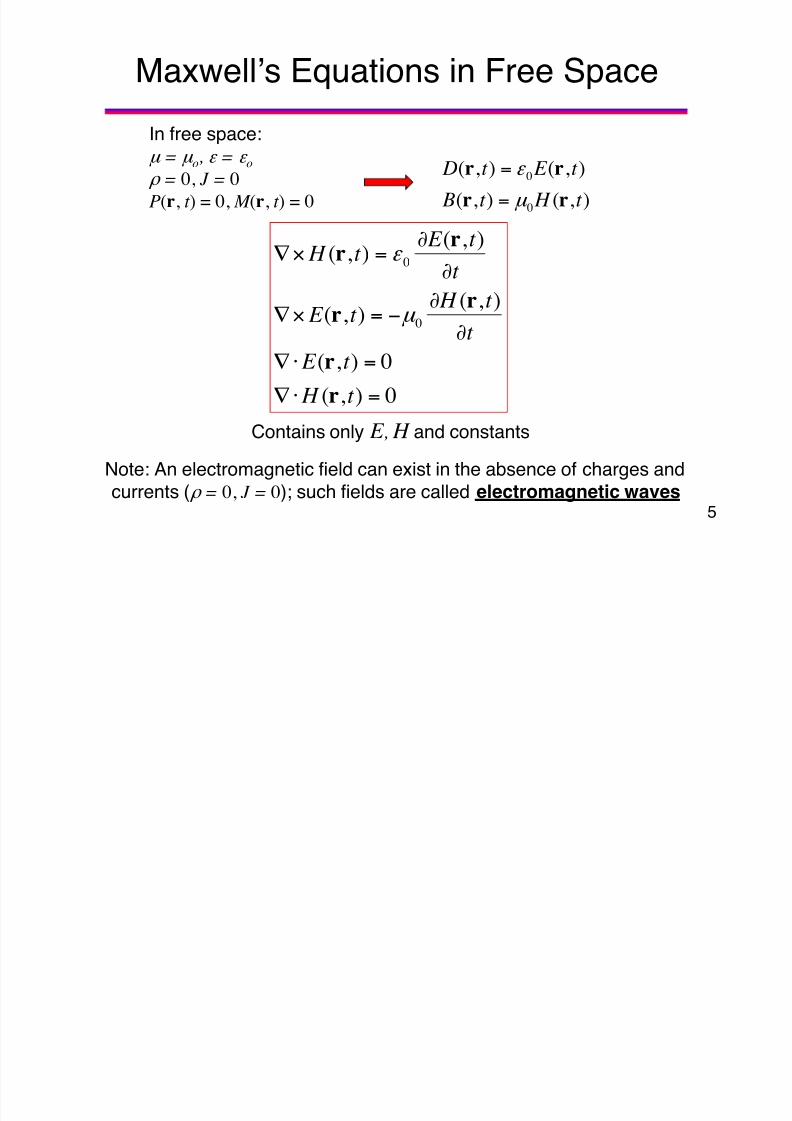
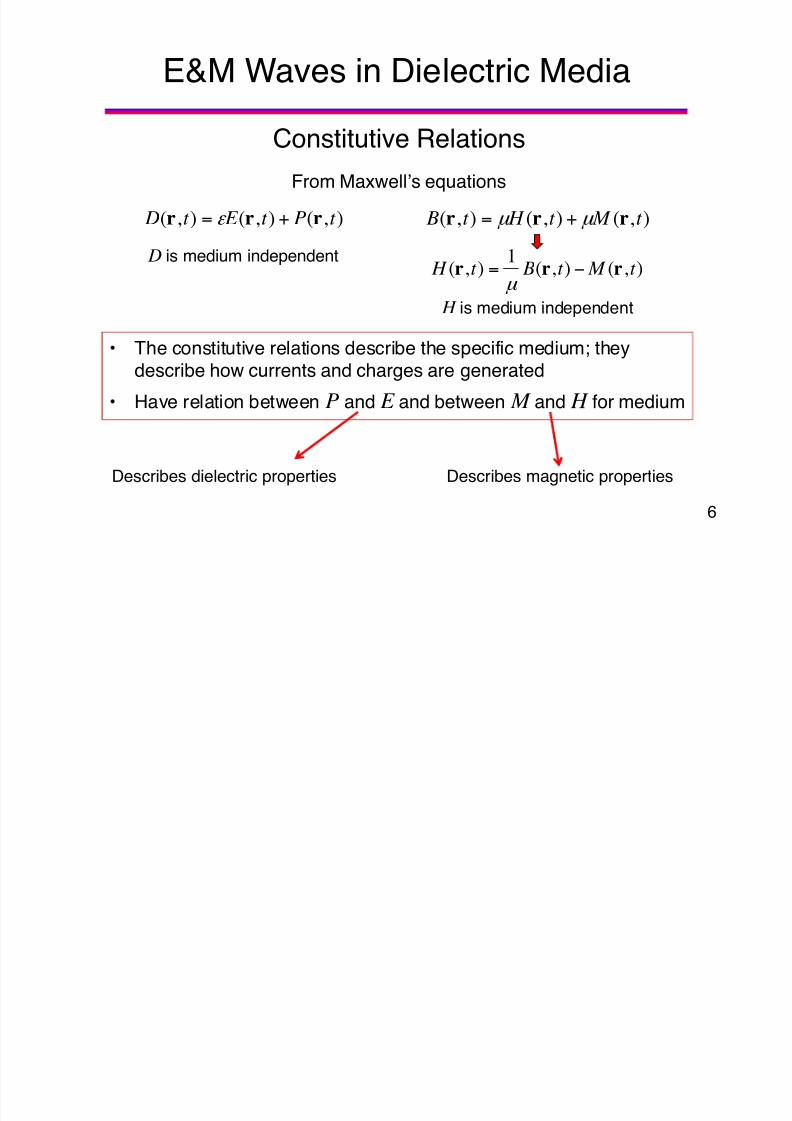
E&M Waves in Dielectric Media
• The constitutive relations describe the specific medium; theydescribe how currents and charges are generated
• Have relation between P and E and between M and H for medium
),(),(),( t Pt E t D rrr += ! ),(),(),( t M t H t B rrr µ µ +=
Describes dielectric properties Describes magnetic properties
),(),(
1
),( t M t Bt H rrr '
= µ
H is medium independent
From Maxwell’s equations
D is medium independent
Constitutive Relations
8/10/2019 Introduction to Photonics lecture 13-14-15 16 Electromagnetic Optics(1)
http://slidepdf.com/reader/full/introduction-to-photonics-lecture-13-14-15-16-electromagnetic-optics1 7/59
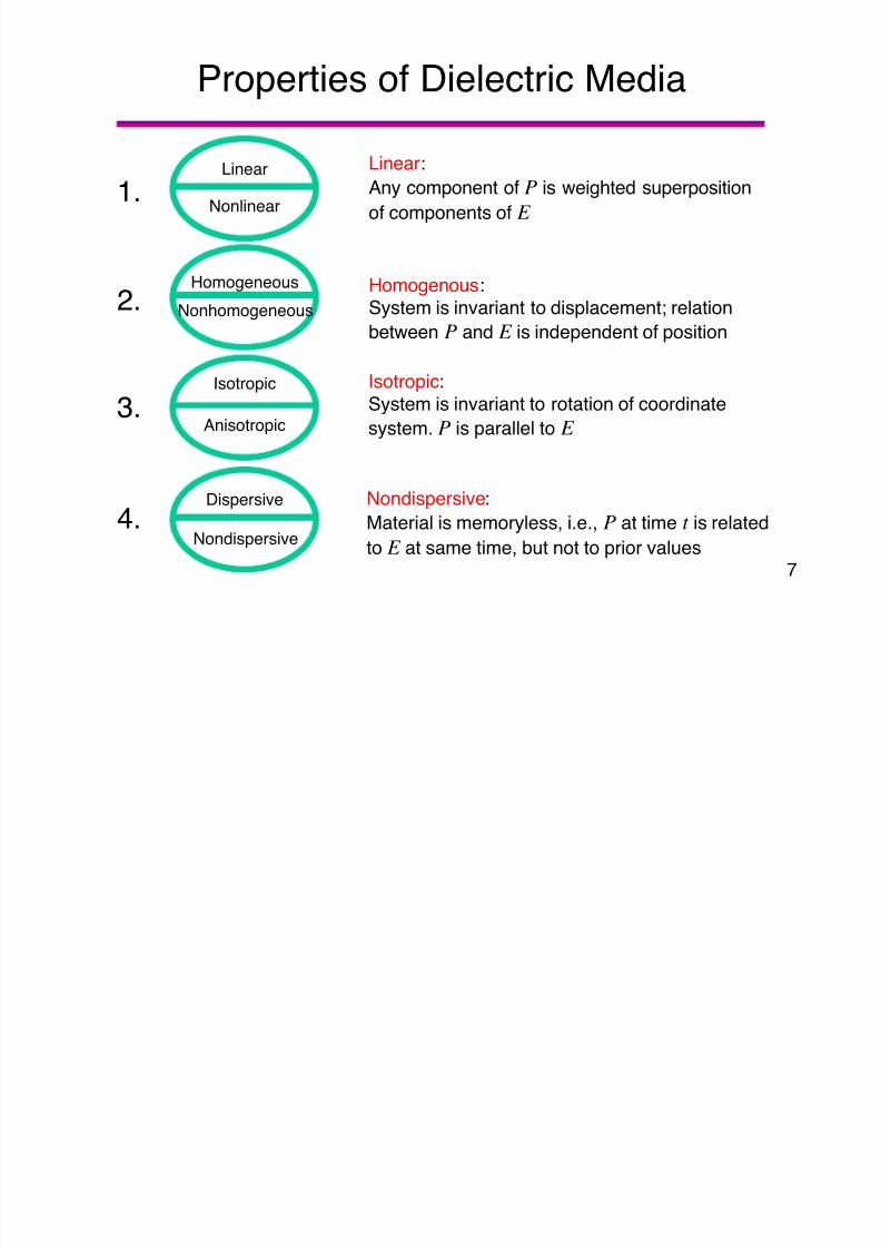
Nondispersive:
Material is memoryless, i.e., P at time t is related
to E at same time, but not to prior values
Linear
Nonlinear1.
Linear:
Any component of P is weighted superposition
of components of E
Nondispersive
Dispersive
4.
Isotropic
Anisotropic3.
Isotropic:System is invariant to rotation of coordinate
system. P is parallel to E
Homogeneous
2.
Homogenous:
System is invariant to displacement; relationbetween P and E is independent of position
Nonhomogeneous
7
Properties of Dielectric Media

8/10/2019 Introduction to Photonics lecture 13-14-15 16 Electromagnetic Optics(1)
http://slidepdf.com/reader/full/introduction-to-photonics-lecture-13-14-15-16-electromagnetic-optics1 8/59
8
Maxwell’s Equations
0),(
),(),(
),(),(
),(),(
),(
=$%
=$%
&
&'=(%
+&
&=(%
t B
t t D
t t Bt E
t J t
t Dt H
r
rr
rr
rr
r
# Divergenceequations
Curlequations
Time-varying displacement (electric
field) and current are accompanied by
rotating magnetic field
Time-varying magnetic fieldaccompanied by rotating electric field
Diverging displacement (electric field)
related to charge (both bound and free)
Diverging magnetic flux densitydoesn’t exist
8/10/2019 Introduction to Photonics lecture 13-14-15 16 Electromagnetic Optics(1)
http://slidepdf.com/reader/full/introduction-to-photonics-lecture-13-14-15-16-electromagnetic-optics1 9/59
9
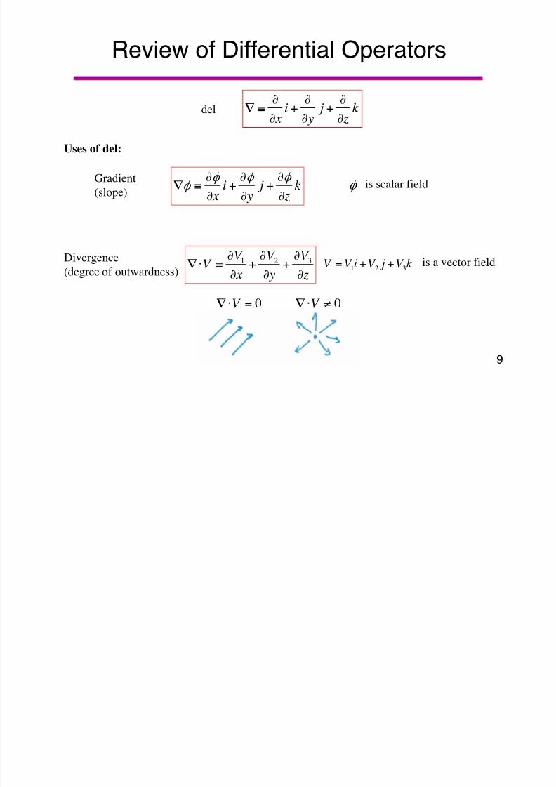
Review of Differential Operators
k z
j y
i x &
&+&
&+&
&)%del
Gradient
(slope) k
z j
yi
x &
&+
&
&+
&
&)%
* * * * * is scalar field
Divergence
(degree of outwardness) z
V
y
V
x
V V
&
&+
&
&+
&
&)$%
321 k V j V iV V 321 ++= is a vector field
Uses of del:
0=$% V 0+$% V
8/10/2019 Introduction to Photonics lecture 13-14-15 16 Electromagnetic Optics(1)
http://slidepdf.com/reader/full/introduction-to-photonics-lecture-13-14-15-16-electromagnetic-optics1 10/59
10
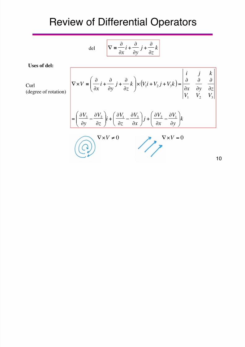
Review of Differential Operators
k z
j y
i x &
&+&
&+&
&)%del
Curl(degree of rotation) ( )
k y
V
x
V j
x
V
z
V i
z
V
y
V
V V V
z y x
k j i
k V j V iV k z j yi xV
!! "
#$$%
&
&
&'
&
&+!
"
#$%
&
&
&'
&
&+!!
"
#$$%
&
&
&'
&
&=
&
&
&
&
&
&
=++(
!! "
#
$$%
&
&
&
+&
&
+&
&)(%
123123
321
321
Uses of del:
0+(% V 0=(% V
8/10/2019 Introduction to Photonics lecture 13-14-15 16 Electromagnetic Optics(1)
http://slidepdf.com/reader/full/introduction-to-photonics-lecture-13-14-15-16-electromagnetic-optics1 11/59
11
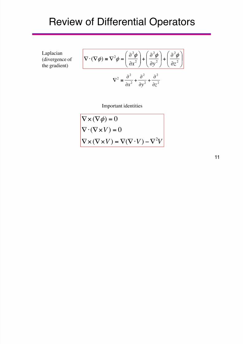
Review of Differential Operators
Laplacian
(divergence of
the gradient)!!
"
#$$%
&
&
&+!!
"
#$$%
&
&
&+!!
"
#$$%
&
&
&=%)%$%
2
2
2
2
2
22)(
z y x
* * * * *
2
2
2
2
2
22
z y x &
&+
&
&+
&
&)%
Important identities
V V V
V 2)()(
0)(
0)(
%'$%%=(%(%
=(%$%
=%(% *

8/10/2019 Introduction to Photonics lecture 13-14-15 16 Electromagnetic Optics(1)
http://slidepdf.com/reader/full/introduction-to-photonics-lecture-13-14-15-16-electromagnetic-optics1 12/59
12
M.E. 1: Ampere’s Law
Displacement current(added by Maxwell)
),(),(
),( t J t
t Dt H r
rr +
&
&=(%
Conductioncurrent
• A time-varying displacement (electric
field) OR current generates magnetic
field with rotation
• Another way to state ‘generates’ is to say ‘is
accompanied by’
• The displacement current term allows forexistence of electromagnetic waves (when
J = 0, E still accompanied by H )
• Recall curl is a measure of field rotation –
how much vector curls around a given point
8/10/2019 Introduction to Photonics lecture 13-14-15 16 Electromagnetic Optics(1)
http://slidepdf.com/reader/full/introduction-to-photonics-lecture-13-14-15-16-electromagnetic-optics1 13/59
13
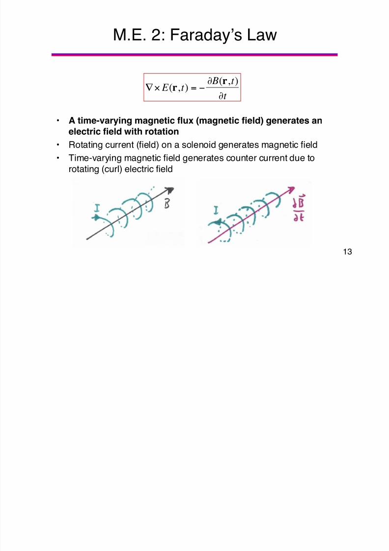
M.E. 2: Faraday’s Law
t
t Bt E
&
&'=(%
),(),( r
r
• A time-varying magnetic flux (magnetic field) generates an
electric field with rotation• Rotating current (field) on a solenoid generates magnetic field
• Time-varying magnetic field generates counter current due to
rotating (curl) electric field

8/10/2019 Introduction to Photonics lecture 13-14-15 16 Electromagnetic Optics(1)
http://slidepdf.com/reader/full/introduction-to-photonics-lecture-13-14-15-16-electromagnetic-optics1 14/59
14
M.E. 3: Gauss’s Law
• The divergence of the electric displacement (electric flux) isproportional to the charge density present at the point
• Mathematical expression for Coulomb’s law
• Relates charge to electric field
• Recall that divergence is a measure of total outgoing flux per unit
volume
),(),( t t D rr # =$%

8/10/2019 Introduction to Photonics lecture 13-14-15 16 Electromagnetic Optics(1)
http://slidepdf.com/reader/full/introduction-to-photonics-lecture-13-14-15-16-electromagnetic-optics1 15/59
15
M.E. 4: Absence of Magnetic Charges
• There are no points in space that act as sources/sinks formagnetic field lines (or magnetic flux)
• Magnetic field lines always close on themselves
• There are no magnetic charges (magnetic monopoles)
0),( =$% t B r

8/10/2019 Introduction to Photonics lecture 13-14-15 16 Electromagnetic Optics(1)
http://slidepdf.com/reader/full/introduction-to-photonics-lecture-13-14-15-16-electromagnetic-optics1 16/59
Introduction to Photonics
Lecture 13/14/15/16: Electromagnetic OpticsNovember 3/5/10/12, 2014
• Electromagnetic theory
• Review of Maxwell’s equations
• Electromagnetic waves in dielectric media
• Conductive media
• Time-harmonic ME and TEM waves
• Absorption and dispersion
• Resonant media and Lorentz model 16
8/10/2019 Introduction to Photonics lecture 13-14-15 16 Electromagnetic Optics(1)
http://slidepdf.com/reader/full/introduction-to-photonics-lecture-13-14-15-16-electromagnetic-optics1 17/59
17
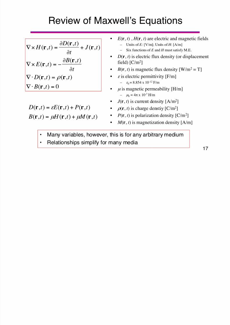
Review of Maxwell’s Equations
• E (r, t ) , H (r, t ) are electric and magnetic fields – Units of E : [V/m]; Units of H : [A/m]
– Six functions of E and H must satisfy M.E.
• D(r, t ) is electric flux density (or displacement
field) [C/m2]
• B(r, t ) is magnetic flux density [W/m2 = T]
• ! is electric permittivity [F/m]
– ! 0 = 8.854 x 10⁻¹² F/m
• µ is magnetic permeability [H/m]
– µ 0 = 4" x 10-7 H/m
• J (r, t ) is current density [A/m2]
• # (r, t ) is charge denstiy [C/m2]
• P(r, t ) is polarization density [C/m2]
• M (r, t ) is magnetization density [A/m]
• Many variables, however, this is for any arbitrary medium
• Relationships simplify for many media
0),(
),(),(
),(),(
),(),(
),(
=$%
=$%
&
&'=(%
+&
&=(%
t B
t t D
t
t Bt E
t J t
t Dt H
r
rr
rr
rr
r
#
),(),(),(
),(),(),(
t M t H t B
t Pt E t D
rrr
rrr
µ µ
!
+=
+=

8/10/2019 Introduction to Photonics lecture 13-14-15 16 Electromagnetic Optics(1)
http://slidepdf.com/reader/full/introduction-to-photonics-lecture-13-14-15-16-electromagnetic-optics1 18/59
Nondispersive:
Material is memoryless, i.e., P at time t is related
to E at same time, but not to prior values
Linear
Nonlinear1.
Linear:
Any component of P is weighted superposition
of components of E
Nondispersive
Dispersive
4.
Isotropic
Anisotropic3.
Isotropic:System is invariant to rotation of coordinate
system. P is parallel to E
Homogeneous
2.
Homogenous:
System is invariant to displacement; relationbetween P and E is independent of position
Nonhomogeneous
18
Properties of Dielectric Media

8/10/2019 Introduction to Photonics lecture 13-14-15 16 Electromagnetic Optics(1)
http://slidepdf.com/reader/full/introduction-to-photonics-lecture-13-14-15-16-electromagnetic-optics1 19/59
Linear, Nondispersive, Homogeneous,
Isotropic Media
%2u - (1/c2)&2u/ &t 2=0 c = (! µ )-1/2 = co /n
, !
! +=== 1
0
0
c
cn
0µ µ =non-magnetic materials:
0
0
0
=$%
=$%
&
&'=(%
&
&=(%
H
E
t
H E
t
E H
µ
!
)1(0
0
, ! !
!
!
+=
=
=
E D
E P
Contains only
E, H fields

8/10/2019 Introduction to Photonics lecture 13-14-15 16 Electromagnetic Optics(1)
http://slidepdf.com/reader/full/introduction-to-photonics-lecture-13-14-15-16-electromagnetic-optics1 20/59
Time-Harmonic Fields
A monochromatic (time-harmonic) field can be written as:
Spatial complex amplitude
])()([2
1})(Re{),(
t j t j t j eeet E - - - '.+== rErErEr
)cos()(
)sin()}(Im{)cos()}(Re{),(
/ -
- -
+=
+=
t
t t t E
rE
rErEr
This is a different way of writing:
where !! "
#$$%
& = '
)}(Re{
)}(Im{tan( 1
rE
rEr)/

8/10/2019 Introduction to Photonics lecture 13-14-15 16 Electromagnetic Optics(1)
http://slidepdf.com/reader/full/introduction-to-photonics-lecture-13-14-15-16-electromagnetic-optics1 21/59
M.E. for Time-Harmonic Fields
Expressed with only complex spatial amplitudes
where complex permittivity is:
0 (1 ) i0
! ! , -
= + +
B
!D
BE
JDH
$%
=$%
'=(%
+=(%
-
-
j
j
MHB
PED
00
0
µ µ
!
+=
+=
8/10/2019 Introduction to Photonics lecture 13-14-15 16 Electromagnetic Optics(1)
http://slidepdf.com/reader/full/introduction-to-photonics-lecture-13-14-15-16-electromagnetic-optics1 22/59
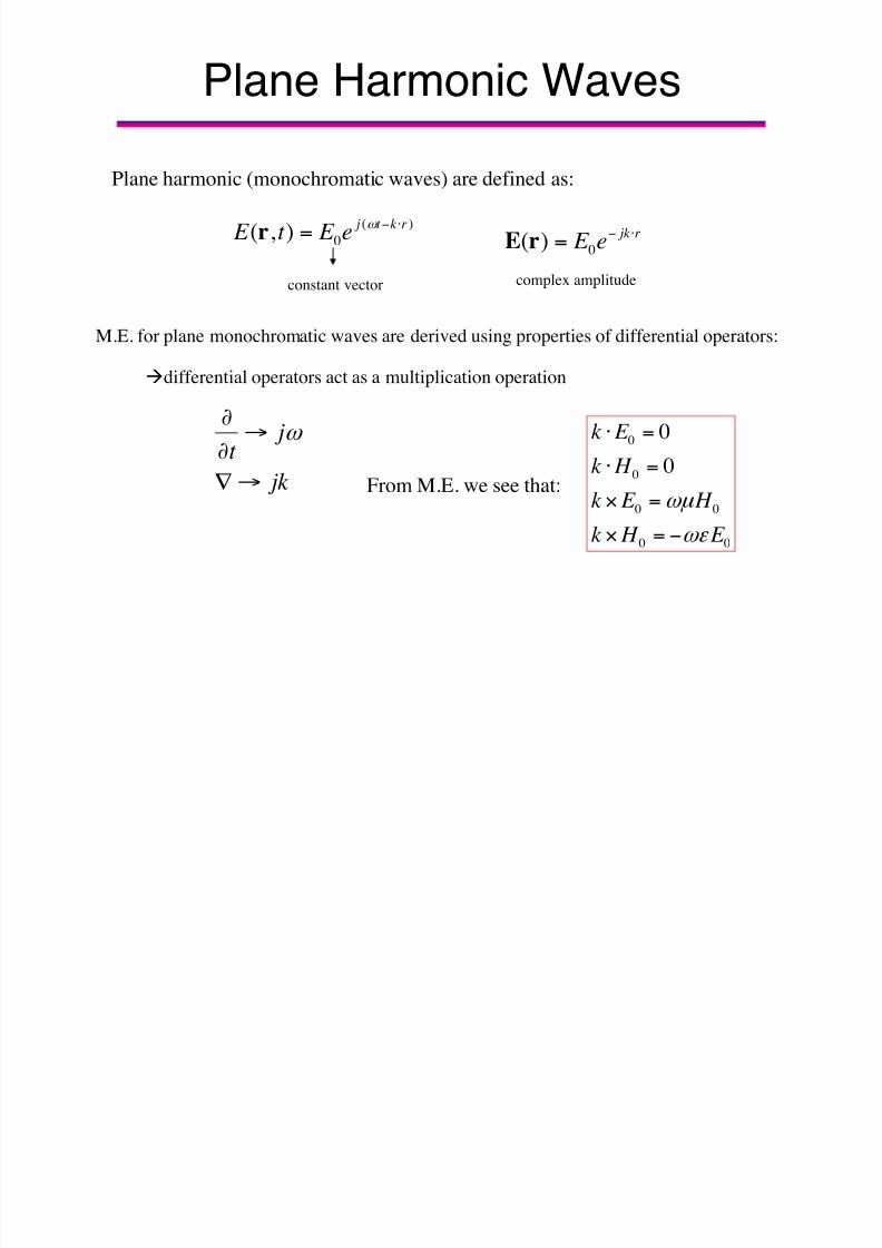
Plane Harmonic Waves
Plane harmonic (monochromatic waves) are defined as:
M.E. for plane monochromatic waves are derived using properties of differential operators:
constant vector
!differential operators act as a multiplication operation
From M.E. we see that:
0
0
0 0
0 0
0
0
k E
k H
k E H
k H E
- µ
-!
$ =
$ =
( =
( = '
)(
0),( rk t j
e E t E $'= -
r r jk e E
$'= 0)(rE
complex amplitude
jk
j t
1%
1&
&-

8/10/2019 Introduction to Photonics lecture 13-14-15 16 Electromagnetic Optics(1)
http://slidepdf.com/reader/full/introduction-to-photonics-lecture-13-14-15-16-electromagnetic-optics1 23/59
Helmholtz Equations
For source-free media, and time-harmonic fields:
Typical scattering problem
0
0
22
22
=+%
=+%
HH
EE
k
k
Vector Helmholtz equations:
! µ - 22 =k
What are the boundary conditions ?
%$%)%2 is a dyadic which, when operated
on a vector yields a vector.
In the special case where E is specified relative to a rectangular
Cartesian coordinate system ! the components of E separatelysatisfy the scalar wave equation:
022 =+% 2 2 k

8/10/2019 Introduction to Photonics lecture 13-14-15 16 Electromagnetic Optics(1)
http://slidepdf.com/reader/full/introduction-to-photonics-lecture-13-14-15-16-electromagnetic-optics1 24/59
0=$%
=$%
B
D
0
3
=$
=$
''
'''''
&
&
V
V V
dAn B
rd dAn D #
( )( ) 012
12
=$'
=$'
n B Bn D D 0
t
B E
t D J H
&
&'=(%
&&+=(%
'''
'''
$! "
#$%
&
&
&'=$
$! "
#$%
&
&
&+=$
&
&
S S
S S
dAnt
Bdl E
dAnt
D J dl H
( )( ) K H H n
E E n
='(
='(
12
12 0
Using the divergence theorem
:K Surface
current density :0 Surface charge
density
Using Stokes’s theorem
Boundary Conditions

8/10/2019 Introduction to Photonics lecture 13-14-15 16 Electromagnetic Optics(1)
http://slidepdf.com/reader/full/introduction-to-photonics-lecture-13-14-15-16-electromagnetic-optics1 25/59
Boundary Conditions
From M.E. 1, 2:
From M.E. 3, 4:
( )( )
0i j
i j
n E E
n H H K
( ' =
( ' =
( )( ) 0
i j
i j
n D D
n B B
0 $ ' =
$ ' =
a surface current
density may be present
a surface charge
density may be present
Tangential components
Condition:
Normal components
Condition:
8/10/2019 Introduction to Photonics lecture 13-14-15 16 Electromagnetic Optics(1)
http://slidepdf.com/reader/full/introduction-to-photonics-lecture-13-14-15-16-electromagnetic-optics1 26/59
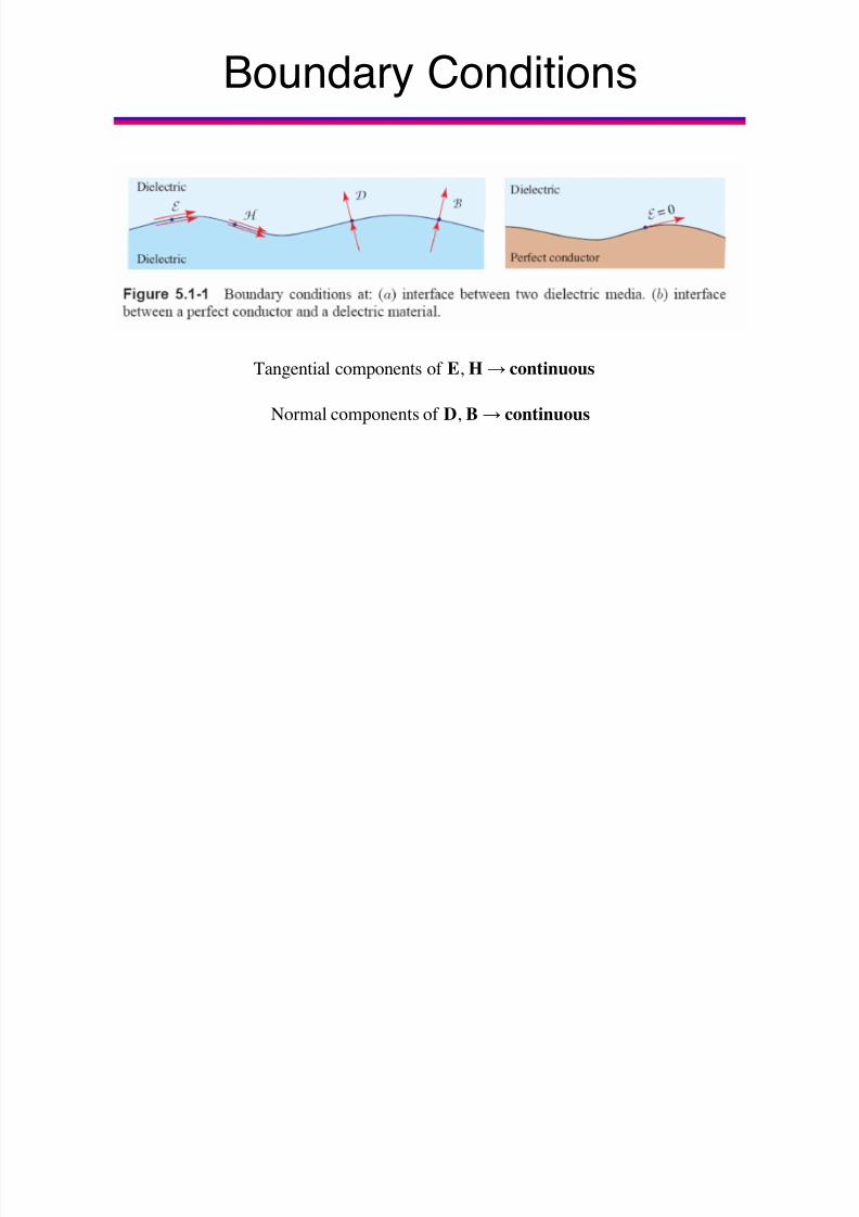
Tangential components of E, H" continuous
Normal components of D, B" continuous
Boundary Conditions

8/10/2019 Introduction to Photonics lecture 13-14-15 16 Electromagnetic Optics(1)
http://slidepdf.com/reader/full/introduction-to-photonics-lecture-13-14-15-16-electromagnetic-optics1 27/59
The simplest solution of Maxwell’s equations in free space is the harmonic transverse
electromagnetic wave (TEM) wave
TEM Wave
3 o = µ o ! o = 377 Ohms
Properties:
• E and H are orthogonal to one another and to the direction of propagation (the z direction)
• The ratio of the magnitudes of E and H is the impedance = 377 Ohms.
z
x
y
E
H
H
z
E
E = E oe j - (t ' z/c o ) ˆ x
H = E o3 o
e j - ( t ' z/ co ) ˆ y
3 o = µ o ! o

8/10/2019 Introduction to Photonics lecture 13-14-15 16 Electromagnetic Optics(1)
http://slidepdf.com/reader/full/introduction-to-photonics-lecture-13-14-15-16-electromagnetic-optics1 28/59
Poynting Vector and Energy Flow
S E H = ( Poynting vector (power flux density, W/cm2)
[ ]1
2W D E B H = $ + $ E&M energy density (J/cm3)
Specifies the transfer rate of E&M energy: of fundamental importance in propagation, absorption, scattering
The rate at which E&M energy is transferred across a general surface:
A
W S ndA= ' $'
Positive if energy is absorbed inside V
For harmonic fields in linear media, the time-averaged Poynting vector is:
{ }1
Re ( ) *( )2
S E r H r= (This is a relevant experimental quantity:=),( t r I
Optical intensity
8/10/2019 Introduction to Photonics lecture 13-14-15 16 Electromagnetic Optics(1)
http://slidepdf.com/reader/full/introduction-to-photonics-lecture-13-14-15-16-electromagnetic-optics1 29/59
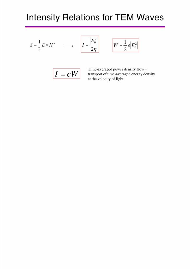
Intensity Relations for TEM Waves
.(= H E S
2
1
3 2
2
0 E I = 2
02
1 E W ! =
cW I =Time-averaged power density flow =
transport of time-averaged energy density
at the velocity of light

8/10/2019 Introduction to Photonics lecture 13-14-15 16 Electromagnetic Optics(1)
http://slidepdf.com/reader/full/introduction-to-photonics-lecture-13-14-15-16-electromagnetic-optics1 30/59
= 4 + j 4 4
k = - ! µ o = 1+ , k o = 1+ 4 , + j 4 4 , k o
k = 5 ' j 12 6 5 ' j 12 6 = k o 1+ 4 , + j 4 4 ,
n ' j 6
2k o= 1+ 4 , + j 4 4 ,
Absorption is governed by a complex susceptibility:
Complex wavenumber
Let
6 = absorption coefficient , attenuation coefficient, or extinction coefficient
U = e' jkz
= e' j ( 5 ' 1
26 ) z
= e' 1
26 z
e' j 5 z I = U
2= e
'6 z
5 = propagation constant = nk o
Expression relating refractive index and
absorption coefficient to complex
susceptibility
z
Attenuated wave
Absorption
then,
Expression for plane wave:
! = ! o(1 + , )Complex permittivity
8/10/2019 Introduction to Photonics lecture 13-14-15 16 Electromagnetic Optics(1)
http://slidepdf.com/reader/full/introduction-to-photonics-lecture-13-14-15-16-electromagnetic-optics1 31/59

8/10/2019 Introduction to Photonics lecture 13-14-15 16 Electromagnetic Optics(1)
http://slidepdf.com/reader/full/introduction-to-photonics-lecture-13-14-15-16-electromagnetic-optics1 32/59
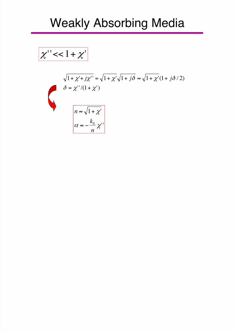
Strongly Absorbing Media
'1'' , , +>>
2/)''(2
2/)''(
0 , 6
,
'8
'8
k
n
00'' >(< 6 Note that
)''()1(2
1)''(''2/ 0 , , , 6 ''±=''=8' j j j k j n
8/10/2019 Introduction to Photonics lecture 13-14-15 16 Electromagnetic Optics(1)
http://slidepdf.com/reader/full/introduction-to-photonics-lecture-13-14-15-16-electromagnetic-optics1 33/59
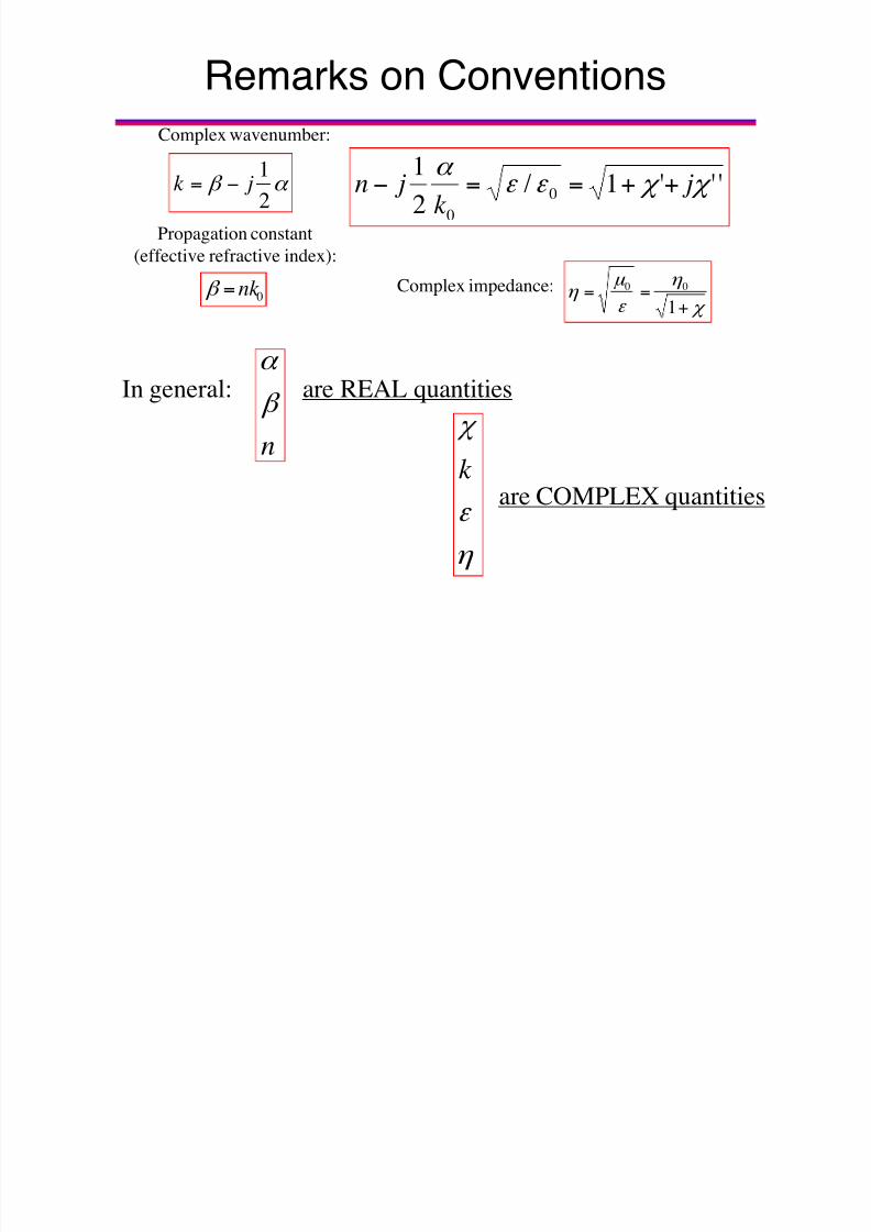
Remarks on Conventions
In general:
n
5
6 are REAL quantities
3
!
k are COMPLEX quantities
'''1/2
10
0
, , ! ! 6
j k
j n ++=='6 5 2
1 j k '=
,
3
!
µ 3
+
==
1
00Complex impedance:0nk = 5
Propagation constant
(effective refractive index):
Complex wavenumber:
8/10/2019 Introduction to Photonics lecture 13-14-15 16 Electromagnetic Optics(1)
http://slidepdf.com/reader/full/introduction-to-photonics-lecture-13-14-15-16-electromagnetic-optics1 34/59
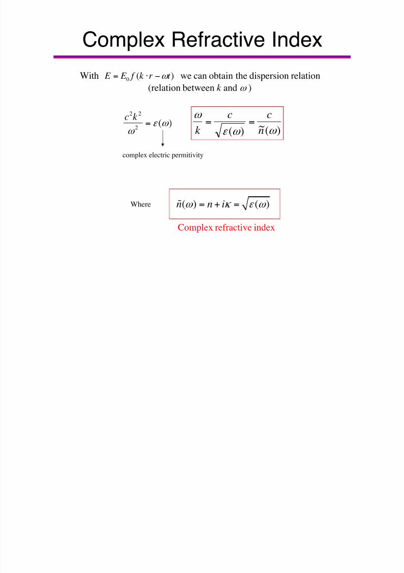
Complex Refractive Index
With 0 ( ) E E f k r t - = $ ' we can obtain the dispersion relation
2 2
2 ( )
c k ! -
- =
complex electric permitivity
( ) ( )n n i- 9 ! - = + =!Where
Complex refractive index
)(~)( - - !
-
n
cc
k ==
(relation between k and - )

8/10/2019 Introduction to Photonics lecture 13-14-15 16 Electromagnetic Optics(1)
http://slidepdf.com/reader/full/introduction-to-photonics-lecture-13-14-15-16-electromagnetic-optics1 35/59
Complex Refractive Index
( ) ( )n n i- 9 ! - = + =!
0
( )n
: :
- =
0
4( ) ( )
" 6 - 9 -
:
=
Snell’s law refractive index
(real dispersion)
Intensity extinction
(energy dissipation)
Re( ) ( ) ph
g
cv
k n
vk
-
-
-
= =
&=
&
Absorption coefficient
)(~)( - - !
- n
cck
==
8/10/2019 Introduction to Photonics lecture 13-14-15 16 Electromagnetic Optics(1)
http://slidepdf.com/reader/full/introduction-to-photonics-lecture-13-14-15-16-electromagnetic-optics1 36/59
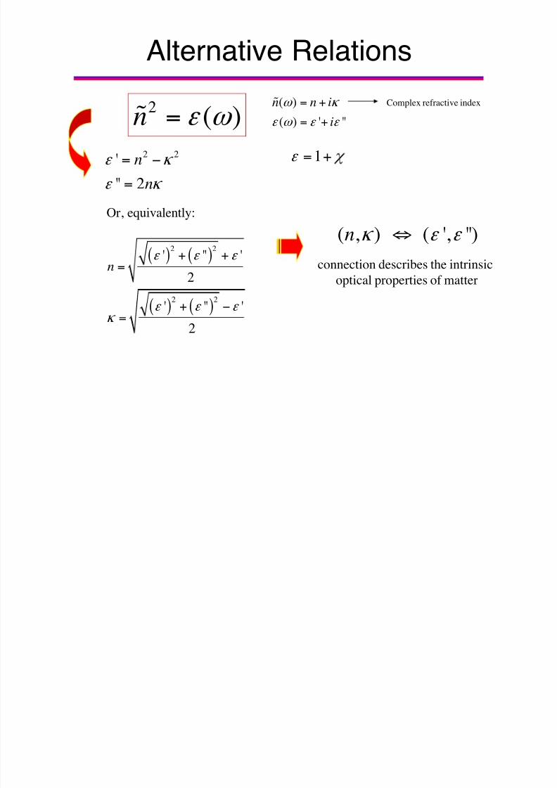
Alternative Relations
2 ( )n ! - =! ( )
( ) ' ''
n n i
i
- 9
! - ! !
= +
= +
!
2 2'
'' 2
n
n
! 9
! 9
= '
=
( ) ( )
( ) ( )
2 2
2 2
' '' '
2
' '' '
2
n! ! !
! ! ! 9
+ +=
+ '=
Or, equivalently:
( , ) ( ', '')n 9 ! ! ;
connection describes the intrinsic
optical properties of matter
! +=1
Complex refractive index

8/10/2019 Introduction to Photonics lecture 13-14-15 16 Electromagnetic Optics(1)
http://slidepdf.com/reader/full/introduction-to-photonics-lecture-13-14-15-16-electromagnetic-optics1 37/59
Kramers-Kronig Relations
Hilbert transform pairs
For any linear, shift-invariant, causal system with real impulse-response functions,
, ’ and , ’’ are related through Kramers-Kronig relations:
Kramers-Kronig relations for n and 6
Relation between absorption and dispersion: if n(: )!
then 6 (: )
8/10/2019 Introduction to Photonics lecture 13-14-15 16 Electromagnetic Optics(1)
http://slidepdf.com/reader/full/introduction-to-photonics-lecture-13-14-15-16-electromagnetic-optics1 38/59
Optical Transmission

8/10/2019 Introduction to Photonics lecture 13-14-15 16 Electromagnetic Optics(1)
http://slidepdf.com/reader/full/introduction-to-photonics-lecture-13-14-15-16-electromagnetic-optics1 39/59
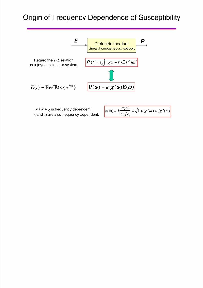
P
Origin of Frequency Dependence of Susceptibility
Regard the P-E relation
as a (dynamic) linear system
!Since , is frequency dependent,
n and 6 are also frequency dependent.n(- ) ' j 6 (- )
2- co
= 1 + 4 , (- )+ j 4 4 , (- )
P (t ) =! o ' , (t ' 4 t )E ( 4 t )d 4 t
Dielectric mediumLinear, homogeneous, isotropic
})(Re{)( t j et E - - E= )()()( 0 - -- - - -- - ! !! ! - -- - EP =

8/10/2019 Introduction to Photonics lecture 13-14-15 16 Electromagnetic Optics(1)
http://slidepdf.com/reader/full/introduction-to-photonics-lecture-13-14-15-16-electromagnetic-optics1 40/59
LSI Systems and Dielectric Media
Electric dipole
)(t P : response (real)
)(t E : input (real)
)(0 t ! : impulse-response (real)
)(0 < ! : transfer function
*)()( < , < , =' : Hermitian symmetry
P ( t ) =! o ' , (t ' 4 t )E ( 4 t )d 4 t
)(t 7
Recall LSI = linear, shift-invariant
P P = - Nex
N : atomic density
-e: electronic charge
x: charge displacement
8/10/2019 Introduction to Photonics lecture 13-14-15 16 Electromagnetic Optics(1)
http://slidepdf.com/reader/full/introduction-to-photonics-lecture-13-14-15-16-electromagnetic-optics1 41/59
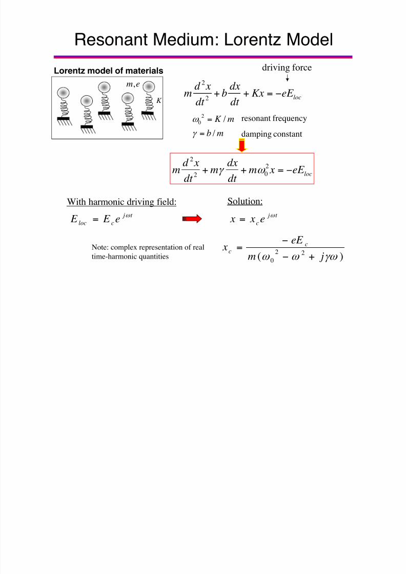
Resonant Medium: Lorentz Model
NpP
ex p
=
'= induced dipole moment/atom
(-e = electron charge; x = displacement)
polarization density
( N = atomic density)
Lorentz model of materials
K
,m e“There is not a single granule oflight which is not the fruit of an
oscillating charge.” - A. Lorentz
How do we model the dipole moment (of an atom) induced by incident electric field?
! model motion of bound charge as driven harmonic oscillator
t j
cloc e E E
-
= : local electric field that induces dipole moment

8/10/2019 Introduction to Photonics lecture 13-14-15 16 Electromagnetic Optics(1)
http://slidepdf.com/reader/full/introduction-to-photonics-lecture-13-14-15-16-electromagnetic-optics1 42/59
Lorentz model of materials
K
,m e
With harmonic driving field:
2
0 /
/
K m
b m
-
=
=
=
driving force
Solution:
Resonant Medium: Lorentz Model
loceE Kxdt
dxb
dt
xd m '=++
2
2
damping constant
resonant frequency
loceE xmdt
dxm
dt
xd m '=++ 2
02
2
- =
t j cloc e E E - = t j
c e x x - =
)( 22
0 =- - - j m
eE x c
c+'
'=Note: complex representation of real
time-harmonic quantities

8/10/2019 Introduction to Photonics lecture 13-14-15 16 Electromagnetic Optics(1)
http://slidepdf.com/reader/full/introduction-to-photonics-lecture-13-14-15-16-electromagnetic-optics1 43/59
43
loceE xm
dt
dxm
dt
xd m '=++ 2
02
2
- =
Resonant Medium: Lorentz Model
mass*
acceleration
Where does this come from?
restore frictionexternaltotal
total
F F F F
maF
++=
= Newton’s Law
Driving force from
electric field of
incident wave
Friction/damping
(loss: due to
emission,
scattering/
collisions)
Restoring
force
8/10/2019 Introduction to Photonics lecture 13-14-15 16 Electromagnetic Optics(1)
http://slidepdf.com/reader/full/introduction-to-photonics-lecture-13-14-15-16-electromagnetic-optics1 44/59
Collection of Oscillators
Induced dipole moment of an oscillator is:
Polarization density of medium containing N oscillators/unit volume is:
Where we have defined the plasma frequency:
22
0
p
Ne
m-
! =
0P E ! , =
ex p '=
Nex NpP '==
E j
P p
022
0
2
! =- - -
- +'
=
Recall:=- - -
- ,
j
p
+'=
22
0
2

8/10/2019 Introduction to Photonics lecture 13-14-15 16 Electromagnetic Optics(1)
http://slidepdf.com/reader/full/introduction-to-photonics-lecture-13-14-15-16-electromagnetic-optics1 45/59
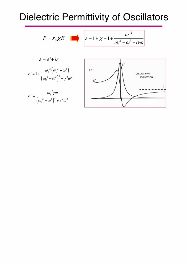
Dielectric Permittivity of Oscillators
2
2 2
0
1 1 p
i
- ! , - - =-
= + = +' '
' ''i! ! ! = +
( )( )
( )
2 2 2
0
22 2 2 2
0
2
22 2 2 2
0
' 1
''
p
p
- - - !
- - = -
- =- !
- - = -
'= +
' +
=
' +
1
0P E ! , =
8/10/2019 Introduction to Photonics lecture 13-14-15 16 Electromagnetic Optics(1)
http://slidepdf.com/reader/full/introduction-to-photonics-lecture-13-14-15-16-electromagnetic-optics1 46/59
8/10/2019 Introduction to Photonics lecture 13-14-15 16 Electromagnetic Optics(1)
http://slidepdf.com/reader/full/introduction-to-photonics-lecture-13-14-15-16-electromagnetic-optics1 47/59
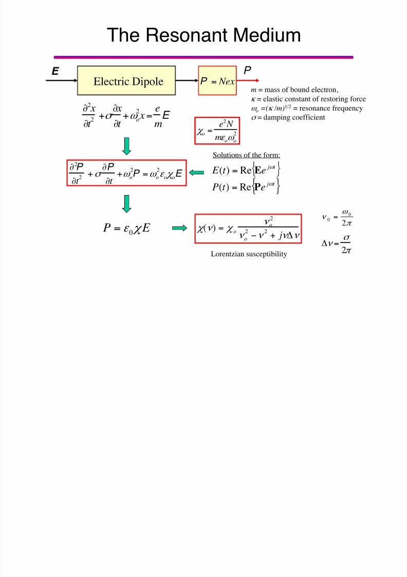
The Resonant Medium
&2 x
&t 2 +0
& x
&t +- o
2 x=
e
mE
, (< ) = , o< o
2
< o2
' < 2+ j < ><
P
&2P
&t 2 +0
&P
&t +- o
2P =- o
2! o , oE
, o = e2 N
m! o- o2
Electric Dipole
>< = 0
2" Lorentzian susceptibility
m = mass of bound electron,
9 = elastic constant of restoring force
- o =(9 /m)1/2 = resonance frequency
0 = damping coefficient
Solutions of the form:
{ }t j
t j
et P
et E
-
-
P
E
Re)(
Re)(
=
=
P = Nex
0P E ! , = "
- < 2
00 =
8/10/2019 Introduction to Photonics lecture 13-14-15 16 Electromagnetic Optics(1)
http://slidepdf.com/reader/full/introduction-to-photonics-lecture-13-14-15-16-electromagnetic-optics1 48/59
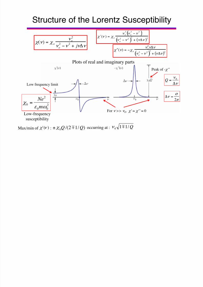
Structure of the Lorentz Susceptibility
<
<
>= 0Q
" <
2=>
Low frequency limit
)/12/(0 QQ "±Max/min of :)(' < , occurring at : Q/110 "<
2
00
2
0
- !
,
m
Ne=
Low-frequency
susceptibility
, (< ) = , o< o
2
< o2
' < 2+ j < ><
Plots of real and imaginary parts
Peak of - , ’’
For < >> < 0, , ’ 8 , ’’ 8 0
4 , (< ) = , o
< o2
< o2
' < 2( )
< o
2' < 2( )
2+ < >< ( )2
4 4 , (< ) = ' , o< o
2< ><
< o2
' < 2( )2
+ < >< ( )2

8/10/2019 Introduction to Photonics lecture 13-14-15 16 Electromagnetic Optics(1)
http://slidepdf.com/reader/full/introduction-to-photonics-lecture-13-14-15-16-electromagnetic-optics1 49/59

8/10/2019 Introduction to Photonics lecture 13-14-15 16 Electromagnetic Optics(1)
http://slidepdf.com/reader/full/introduction-to-photonics-lecture-13-14-15-16-electromagnetic-optics1 50/59
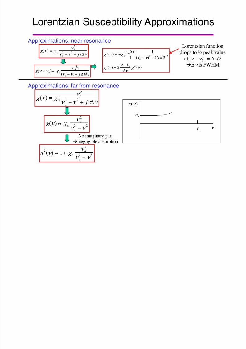
Dielectric Permittivity Approximations
For frequencies in the vicinity of 0-
( )
( ) ( )
( ) ( )
0 0
2 2
0
0
2 2
0
/ 2' 1
/ 2
/ 4''
/ 2
p
p
- - - - !
- - =
=- - !
- - =
'8 +
' +
8
' +
2
pmax
0
0
max max
min max
''
FWHM( '') / 2
' 1 '' / 2
' 1 '' / 2
- ! =-
! - - =
! !
! !
8
1 ' = ±
= +
= 'Lorentzian lineshape
(

8/10/2019 Introduction to Photonics lecture 13-14-15 16 Electromagnetic Optics(1)
http://slidepdf.com/reader/full/introduction-to-photonics-lecture-13-14-15-16-electromagnetic-optics1 51/59
Absorption/Refraction
One resonance
(dilute concentration
of atoms)
Multiple resonances
(different lattice and
electronic vibrations)
! Overall susceptibility
from superposition of
resonances
'''1/2
10
0 , , ! !
6 j k j n ++=='
Recall: , ’’ confined near
resonances; , ’ near and
below resonance
!Absoption anddispersion strong near
resonance;
Away from resonance n
constant (nondispersive,
nonabsorptive)

8/10/2019 Introduction to Photonics lecture 13-14-15 16 Electromagnetic Optics(1)
http://slidepdf.com/reader/full/introduction-to-photonics-lecture-13-14-15-16-electromagnetic-optics1 52/59
Transparent [in Visible]
Although medium is approximately nondispersive/nonabsorptive away from resonance,
each resonance contributes to value of refractive index away from [below] resonance
Recall Kramers-Kronig relations:

8/10/2019 Introduction to Photonics lecture 13-14-15 16 Electromagnetic Optics(1)
http://slidepdf.com/reader/full/introduction-to-photonics-lecture-13-14-15-16-electromagnetic-optics1 53/59
Absorption/Refraction
One resonance
(dilute concentration
of atoms)
Multiple resonances
(different lattice and
electronic vibrations)
! Overall susceptibility
from superposition of
resonances
'''1/2
10
0 , , ! !
6 j k j n ++=='
Recall: , ’’ confined near
resonances; , ’ near and
below resonance
!Absoption anddispersion strong near
resonance;
Away from resonance n
constant (nondispersive,
nonabsorptive)

8/10/2019 Introduction to Photonics lecture 13-14-15 16 Electromagnetic Optics(1)
http://slidepdf.com/reader/full/introduction-to-photonics-lecture-13-14-15-16-electromagnetic-optics1 54/59
The Sellmeier Equation (far from resonance)!susceptibility is a sum of terms
Media with multiple resonances
n2(: ) 8 1 + , i
: 2
: 2
' : i2
i
)
n28 1+ , oi
< i2
< i2
' < 2
i)
• Electronic vibrations• Lattice vibrations
Superpositionof different contributions
The imaginary part is confined near resonance
The real part contributes at all frequencies
The Sellmeier Equation
oi
8/10/2019 Introduction to Photonics lecture 13-14-15 16 Electromagnetic Optics(1)
http://slidepdf.com/reader/full/introduction-to-photonics-lecture-13-14-15-16-electromagnetic-optics1 55/59
N = n ' : dn
d : D: = ' :
c
d 2n
d : 2
= group index
c/N = group velocity
= dispersion coefficient(ps/km-nm)
Refractive Index of Silica Glass in the Transparent Region
(well described by three resonances)
, 1=.6961663; : 1 =.0684043 µm
, 2 =0.4079426; : 2 =0.1162414 µm
, 3 =0.89794; : 3 =9.896161 µmn 2(: ) 8 1 + , i
: 2
: 2
' : i2
i)
D :
n
N

8/10/2019 Introduction to Photonics lecture 13-14-15 16 Electromagnetic Optics(1)
http://slidepdf.com/reader/full/introduction-to-photonics-lecture-13-14-15-16-electromagnetic-optics1 56/59
Refractive Index Dispersion

8/10/2019 Introduction to Photonics lecture 13-14-15 16 Electromagnetic Optics(1)
http://slidepdf.com/reader/full/introduction-to-photonics-lecture-13-14-15-16-electromagnetic-optics1 57/59

8/10/2019 Introduction to Photonics lecture 13-14-15 16 Electromagnetic Optics(1)
http://slidepdf.com/reader/full/introduction-to-photonics-lecture-13-14-15-16-electromagnetic-optics1 58/59
58
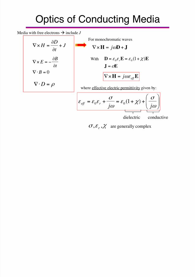
Optics of Conducting Media
EH eff j -! =(%
0µ ! - eff k =
Describes wave propagation with
eff !
µ 3 0=
n and 6 determined from
00 /2/ ! ! 6 eff k j n ='-
0 ! ! !
j reff += 0
When conductive effects dominate
-
0 !
j eff 8
0 - µ 3
0 - µ 6
-! 0
2/)1(
2
2/
0
0
0
j
n
+8
8
8
, where

8/10/2019 Introduction to Photonics lecture 13-14-15 16 Electromagnetic Optics(1)
http://slidepdf.com/reader/full/introduction-to-photonics-lecture-13-14-15-16-electromagnetic-optics1 59/59
Physical Meaning
Where complex permittivity defined as:
bound charge current density
free charge current density
Im( ) Im( ) Re 0
! , -
& #= + $ !
% "
Both conductivity and susceptibility contribute to the imaginary part of the permittivity
If the imaginary parts of µ or ! are nonzero, the amplitude of a plane wave will
decrease as it propagates in the medium! absorption
Complex phenomenological coefficients of a medium are equivalent to a phase
difference between P and E (or H and B) and are manifested by absorption
! "
#$%
& ++=
-
0 , ! ! j )1(0