Technical report, IDE0891 , November 17, 2008

Introduction to Parabolic DifferentialEquations

Catherine Bandle

Mathematisches Institut, Universitat Basel

Rheinsprung 21, CH-4051 Basel, Switzerland

catherine.bandle@unibas.ch

School of Information Science, Computer and Electrical EngineeringHalmstad University

Contents

1 Some results for ordinary differential equation 3

2 Partial differential equations 62.1 Introduction . . . . . . . . . . . . . . . . . . . . . . . . . . . . . . . . . . . 62.2 Reaction-diffusion equations . . . . . . . . . . . . . . . . . . . . . . . . . . 7

2.2.1 . . . . . . . . . . . . . . . . . . . . . . . . . . . . . . . . . . . . . . 72.2.2 The balance equation . . . . . . . . . . . . . . . . . . . . . . . . . . 7

2.3 Simple observations . . . . . . . . . . . . . . . . . . . . . . . . . . . . . . . 10

3 Construction of a fundamental solution 11

4 Initial value problem (Cauchy problem) 134.1 Nonhomogeneous problem . . . . . . . . . . . . . . . . . . . . . . . . . . . 14

5 Separation of variables 15

6 Boundary conditions 166.1 Inhomogeneous problem . . . . . . . . . . . . . . . . . . . . . . . . . . . . 17

7 Maximum principle 187.1 Applications . . . . . . . . . . . . . . . . . . . . . . . . . . . . . . . . . . . 19

7.1.1 Uniqueness . . . . . . . . . . . . . . . . . . . . . . . . . . . . . . . 197.1.2 Estimates . . . . . . . . . . . . . . . . . . . . . . . . . . . . . . . . 20

8 Viscosity solutions 21

9 Parabolic equations of more general type 24

10 Weak solution 2510.1 Small excursion to functional analysis . . . . . . . . . . . . . . . . . . . . . 2510.2 Generalized derivatives . . . . . . . . . . . . . . . . . . . . . . . . . . . . . 2610.3 Sobolev spaces . . . . . . . . . . . . . . . . . . . . . . . . . . . . . . . . . 2710.4 Definition of weak solutions . . . . . . . . . . . . . . . . . . . . . . . . . . 27

11 Galerkin approximation 28

1

Preface

This lecture course gives a short introduction into the theory of parabolic differentialequations. It is part of the lecture course Introduction to Financial Mathematics.The main lecture course contains two parts, one of them devoted to the Probability the-ory (15 lectures and classroom exercises) and the second one to the Theory of parabolicequations, which includes 5 lectures devoted to analytical questions and 10 lectures de-voted to numerical methods. This text provides just these 5 lectures devoted to analyticalproperties of solutions which are the most important for applications.We started 2006 a one year master program Master in Financial Mathematics. Theprogram attracted a lot of students from abroad which have quite different preliminaryeducation in the Theory of parabolic equations or Stochastics. Because the well knownBlack-Scholes model and its generalizations are parabolic equations we decided to developsuch introductory course to give the students a possibility to consolidate their knowledgeon this area.We are very glad that Professor Catherine Bandle (Basel, Switzerland) was able to findtime and possibility to came to Halmstad and provide for our students this course.

Ljudmila A. BordagProfessor in Applied MathematicsDirector of the programMaster in Financial MathematicsHalmstad UniversityHalmstad, 2008

2

1 Some results for ordinary differential equation

An ordinary differential equation is a relation of the form

F (u(n)(t), u(n−1)(t), . . . , u(t), u(t), t) = 0, (1)

where t ∈ R is a variable and u(t) is a real valued function, u(n)(t) = dnudtn

and u = dudt

. Thehighest derivative n is called the order of the differential equation. Solving a differentialequation means finding a continuous function u(t) satisfying (1) pointwise.

First order equationsF (u, u, t) = 0. (2)

The first order equations are used to describe a relation between the growth rate of aquantity, u(t) in terms of the quantity at a fixed time t. One of the simplest evolutionlaws is the organic growth

du

dt= a u, u(t) = ceat.

c is an arbitrary parameter which can be determined by prescribing an initial condition

u(t0) = u0.

More generally the growth rate of a substance depending only on the time and the totalquantity at time t can be expressed as a first order differential equation of the type

du

dt= f(t, u(t)). (3)

If f(t, u) > 0 particle produce new substance (source) whereas if f(t, u) < 0 then particlesabsorb the substance (sink). This equation yields a direction field in which the curve u(t)has to be fitted.

3

Definition 1 (3) is called linear if it is of the form

u(t) = a(t)u(t) + b(t).

It is a homogeneous equation if b(t) = 0 otherwise it is called an inhomogeneous equation.

If uh is a solution of the homogeneous equation then the same is true for any multiplecuh.

Every solution of a linear equation can be represented as

u(t) = up(t) + uh(t),

where up is a particular solution of the inhomogeneous and uh is a solution of the ho-mogeneous problem. The general solution of the homogeneous problem can be expressedas

uh(t) = e∫ tt0

a(s)dsc, c ∈ R arbitrary constant number

4

By means of the variation of constants we find

up(t) =

∫ t

t0

e∫ t

τ a(s) dsf(τ) dτ.

Observation The solution of the linear problem is uniquely determined if we prescribean initial condition u(t0) = u0.

General existence and uniqueness result

Definition 2 A function f : U → W, U ⊂ R2, W ⊂ R satisfies a Lipschitz condition

with respect to u if there exist a constant L > 0 such that

|f(t, u1) − f(t, u2)| ≤ L|u1 − u2|

for all (t, u1) , (t, u2) ∈ U

Theorem 3 Let the function f(t, u) be a continuous in some set U = {(t, u) : |t − t0| < a, |u − u0| < b}.Assume that it satisfies a Lipschitz condition in U with respect to u. Then the initial valueproblem

u(t) = f(t, u(t)), u(t0) = u0

has a unique solution in the interval t0 − α ≤ t ≤ t0 + α, α = min(a, b‖f‖∞ ), where

‖f‖∞ = maxU |f |

Remarks

1. The fact that u can be expressed uniquely as a function of u and t is crucial for thevalidity of Theorem 3.

Example where this is not the case: |u| = 1. The solution of the initial value problemis not unique (cf. figure).

2. If in Theorem 3 the function f is only continuous and not Lipschitz, there still existsa solution, but it is not necessarily unique.

Examples. u = up, 0 < p < 1 , u(0) = 0.

5

Problems

1. Construct the direction fields of

u(t) = eu(t), u(t) = u(t)(1 − u(t)).

2. Solve the two equations. Plot the solutions through (0, 0.5). Discuss the long timebehavior of the solutions.

3. Plot the nonlinearity f(u) = u(1 − u). Discuss the role of this function for thesolution computed above. When does it have the role of a source or a sink?

4. The existence theorem guarantees the existence of local solutions, i.e. solution ina neighborhood of t0. Show by means of the equation u(t) = 1 + u2(t) that allsolutions cease to exist after a finite time.

ReferencesE. A. Coddington and N. Levinson, Theory of Ordinary Differential Equations, (1955)P. Hartman, Ordinary Differential Equations, (1982)

2 Partial differential equations

2.1 Introduction

Let u : R × RN → R be a function which depends on the time t and the space variable

x = (x1, x2, . . . , xN ). Its first order partial derivatives are

uxi= lim

h→0

u(t, x1, . . . , xi + h, . . . , xn) − u(x, t)

h, ut = lim

h→0

u(t + h, x) − u(x, t)

h.

The gradient ∇u is a vector pointing in the direction of biggest increase of the functionu(t, ·). It is given by

∇u(t, ·) = (ux1, ux2, . . . , uxN).

Partial derivatives of the second order are defined recursively by

uxit = (uxi)t, uxjxi

= (uxi)xj

, utt = (ut)t,

and similarly higher order derivatives. An equation of the form

F (t, x, u, uxi, ut, uxixj

, utxi) = 0, i = 1, . . . , N, j = 1, . . . , N,

is called a partial differential equation of the second order.

We shall deal with partial differential equations of the form

ut =n∑

i=1

uxixi

︸ ︷︷ ︸

△u

+f(t, x, u, uxi), i = 1, . . . , N.

6

△u is called the Laplacian of u. This equation is an example of a parabolic differentialequation.

Problems

1. Let f(x) = 3x21 + 5x1x

32

Compute∇f(x), △f(x).

2. If u(x, t) is a solution of the heat equation ut = △u, prove that v(t, x) = eαtu(x, t)is a solution of vt = △v + αv.

3. If u(x, t) solves ut = △u, what kind of equation does v(t, x) = u(−t, x) solve?

2.2 Reaction-diffusion equations

2.2.1

Diffusion mechanism models the movement of a substance (population) in a media (envi-ronment).

Let u : R × D → R+ be a function representing for instance the density of the

population or of a substance.Our goal is to know how u(x, t) changes as time evolves and as the location x varies. Wehave three possibilities

1. particles can produce new individuals or kill existing ones (reaction)

2. particles can move around (diffusion)

3. both cases occur (reaction-diffusion) .

The case of pure reaction can be modeled by a ordinary differential equation as we haveseen in Section 1.

2.2.2 The balance equation

We want to express the change of the total mass in D ⊂ RN per unit time, i.e.

d

dt

∫

D

u(x, t)dx, dx = dx1 · . . . · dxn

in terms of diffusion and reaction. We shall make the assumption that the particles obeythe

Fick’s Law Particles move from high density place to a low density place.

Special case: n=1

7

The balance equation in the interval (x, x + dx) is per unit time

ut(t, x)dx︸ ︷︷ ︸

rate of total mass

= σ(x + dx)ux(t, x + dx) − σ(x)ux(t, x)︸ ︷︷ ︸

diffusion through endpoints

+ f(t, u, u, ux)dx︸ ︷︷ ︸

production rate

,

whence

ut(x, t) = (σ(x)ux)x(t, x) + f(t, x, u, ux). (4)

General case

We consider a flux density ~fl = −σ(x)∇u(x, t) where σ(x) > 0 is the diffusion coeffi-cient. In accordance with Fick’s law it points in the direction of the lowest density. Thetotal flux through the boundary ∂D of D is

∫

∂D

(~fl, ~n)dS, ~n outer normal, (·, ·) scalar product.

The balance law reads as

d

dt

∫

D

u(x, t)dx =

∮

∂D

σ(x)∂u

∂ndS +

∫

D

f(x, t, u(x, t),∇u(x, t))dx,

where f(x, t, u,∇u) is a measure for the production ( f > 0) or absorption (f < 0) perunit volume element. The divergence theorem implies that

∮

∂D

∂u

∂ndS =

∫

D

div(σ∇u)dx,∂

∂nouter normal derivative.

Inserting the last expression into the balance law we obtain

∫

D

∂u(x, t)

∂t=

∫

D

[div(σ(x)∇u(x, t)) + f(x, t, u(x, t),∇u(x, t))] dx.

Since the choice of the region D is arbitrary, we deduce that the differential equation

∂u(x, t)

∂t= div(σ(x)∇u(x, t)) + f(x, t, u(x, t),∇u(x, t)) (5)

holds for any (t, x).

Equation (5) is called reaction diffusion equation. Here div(σ(x)∇u(x, t)) is the diffu-sion term which describes the movement of the individuals, and f(x, t, u(x, t),∇u(x, t)) isthe reaction term which describes the birth-death or reaction occurring inside the habitator reactor.

8

Definition 4 A reaction-diffusion equation of the form

ut = div(σ∇u) + f(x, t)

is called linear. If f = 0 is is homogeneous and otherwise inhomogeneous.

The diffusion coefficient σ(x) is not a constant in general since the environment is usu-ally heterogeneous. But when the region of the diffusion is approximately homogeneous,we can assume that σ(x) ≡ σ0 and can be simplified to

∂u

∂t= σ0∆u + f(x, t, u,∇u)

where ∆u = div(∇u) =n∑

i=1

∂2u∂x2

iis the Laplacian operator. When no reaction takes place,

the equation becomes∂u

∂t= σ0∆u

In classical mathematical physics, the equation ut = ∆u is called heat equation, where uis temperature function. Therefore (5) is often called nonlinear heat equation.

Random walksThe heat equation can also be interpreted as a model for random walks. Suppose that

a walker takes steps of lenght △x to the left or to the right along a line, and after eachtime units, the walker will be with probability 1/2 either at x0−△x or x0 +△x. If P (t, x)denotes the number of walkers at time t and location x then

P (t0 + △t, x0) =1

2P (t0, x0 + △x) +

1

2P (t0, x0 −△x).

By the Taylor expansion:

P (t0 + △t, x0) = P (t0, x0) +∂P

∂t(t0, x0)△t +

1

2

∂2P

∂t2(t0, x0)(△t)2 + · · · ,

1

2P (t0, x0 ±△x) =

1

2P (t0, x0) ±

1

2

∂P

∂x(t0, x0)(△x) +

1

4

∂2P

∂x2(t0, x0)(△x)2 + · · · .

Inserting these expression into the above equation we find

∂P

∂t(t0, x0)△t + · · · =

∂2P

∂x2(t0, x0)(△x)2 + · · · .

Here we have assumed that both △x and △t are small quantities. If in addition we assumethat

(△x)2

2△t→ σ0 as △t, △x → 0,

then we arrive at the one-dimensional diffusion equation

∂P

∂t(t, x) = σ0

∂2P

∂x2(t, x).

ReferencesL.C.Evans, Partial Differential Equations, AMS (1998)E. DiBenedetto, Partial Differential Equations, Birkhauser (1995).

9

2.3 Simple observations

1. Consider the homogeneous diffusion equation ut = ∆u.

• Superposition principleIf u1 and u2 are solutions then αu1 + βu2 is also solution

• translation invarianceu(x + x0, t + t0) = v(x, t) is also a solution

• Scaling invarianceu(λx, λ2t) = v(x, t) is also a solution

• If u = u(x)is independent of t, it is called steady state and satisfies ∆u = 0.Such functions are called harmonic functions.

• The function v(t, x) = u(−t, x) solves the backward diffusion equation

vt + ∆u = 0.

2. Consider the inhomogeneous reaction diffusion equation ut = ∆u + f(x, t).

• The general solution is of the form

u(x, t) = uh(x, t) + up(x, t),

where uh is the general solution of the homogeneous equation and up is aparticular solution of the inhomogeneous equation.

Problems

1. Let f(x) = 3x21 + 5x1x

32

Compute∇f(x), △f(x).

2. If u(x, t) is a solution of the heat equation ut = △u, prove that eαtu(x, t) is a solutionof vt = △v + αv.

3. If u(x, t) solves ut = △u, what kind of equation does v(x, t) = u(x,−t) solve?

4. Let u(x, t) = t(x1 +2x2)3 be a density function. Determine the direction of the flow

according to Fick’s law in x = (1, 1).

10

3 Construction of a fundamental solution

Let us consider u(x, t) solution to the equation ut = ∆u. We will seek for a solution ofthe form

v(ξ) · t−α, where ξ =x√t∈ R

N .

Substituting this into equation, we obtain

−αt−α−1v + ∇vt−α

(

− x

2(√

t)3

)

= t−α−1∆v,

αv +

(

∇v,x

2√

t

)

+ ∆v = 0,

αv +1

2(∇v, ξ) + ∆v = 0.

Suppose now that v(ξ) = v(ρ), where ρ = |ξ|, then

∆v = v′′ +(N − 1)v′

ρ=

1

ρN−1(ρN−1v′)′,

hence, we obtain the following expressions

αv +1

2v′ρ +

1

ρN−1(ρN−1v′)′ = 0,

(ρN−1v′)′ = αvρN−1 +v′

2ρN .

Choose α = N2

1

2(vρN)′ + (ρN−1v′)′ = 0,

1

2vρN + ρN−1v′ = a.

We assume further that a = 0, then

v′

v= −1

2ρ.

The solution of this equation isv = C0e

− 14ρ2

,

and the solution of the diffusion equation is

u(x, t) =C0

tN2

e−|x|2

4t .

11

We want the following normalization

∫

RN

u(x, t)dx = 1 ⇒ C0 =1

(4π)N2

.

Finally

Φ(t, x) =1

(4πt)N2

e−|x|2

4t

Φ(t, x) is called Gaussian kernel.

Important observation Φ(x, t) is the normal distribution with mean 0 and varianceσ2 = 2t

The figure describes the Gaussian kernel at times t = 3, 2, 1 (curve 1,2,3). If t is largethe Gaussian kernel is flat.

12

If t decreases the function is more and more peaked (cf. figure) and tends to a Diracfunction in the limit as t → 0.

4 Initial value problem (Cauchy problem)

We consider the following initial value problem (IP){

ut = ∆u in RN × (0,∞)

u = g(x) in RN × {t = 0}

Because of the translation invariance Φ(x − y, t) is also a solution of the heat equationand by the superposition principle so is the Riemann sum

n∑

i=1

Φ(x − yi, t)g(yi)dyi

13

for fixed dyi, i = 1 · · ·n.. Now we can formulate the theorem

Theorem 5 If g ∈ C(RN) ∩ L∞(RN) then

u(x, t) =

∫

RN

Φ(x − y, t)g(y)dy

is a solution of (IP).

Proof Since Φ(x−y, t) is infinitely differentiable for t > δ > 0 and since all its derivativesdecrease very rapidly as x, y → ∞ we can differentiate

∫

RN

Φ(x − y, t)g(y)dy

under the integral. A straightforward computation, yields

ut −△u =

∫

RN

(Φt −△xΦ)(x − y, t)]g(y) dy.

Keeping in mind that Φ is a solution of the heat equation we can conclude that the sameis true for u .The fact that limt→0 u(x, t) = g(x) is technically more involved. A detailed proof can befound e.g. in the book of Evans on Partial Differential Equations p. 47.

Problems

1. Carry out the details in the proof of Theorem 4.1:

(a) u ∈ C∞(RN × R+).

(b) u solves ut = △u

2. Construct a solution of (IP) in the case where △ is replaced by σ0△, σ0 =const.

4.1 Nonhomogeneous problem

We consider problems of the following type

{

ut − ∆u = f(x, t) in RN × R

+

u(x, 0) = 0

We have seen that

u = u(x, t, s) =

∫

RN

Φ(x − y, t − s)f(s, y)dy

14

is a solution of

ut = ∆u

u(x, s) = f(x, s).

Duhamel’s principle

Let

u(x, t) =

t∫

0

u(x, t, s)ds

Then the following theorem holds.

Theorem 6 If f ∈ C , ft ∈ C , fxi,xj∈ C then u(x, t) is the solution of the inhomoge-

neous problem

Proof Formal differentiation with respect to t implies

ut(x, t) = u(x, t, t) +

∫ t

0

ut(x, t, s) ds = f(x, t) +

∫

RN

Φt(x − y, t − s) dy.

Here we have used the fact that for small time the Gaussian kernel behaves like a Diracfunction,

limt→0

∫

RN

Φ(x, t)f(h(x) dx = f(0).

Moreover, since Φ satisfies the heat equation,

∫

RN

Φt(x − y, t − s) dy = −∫

RN

△xΦt(x − y, t − s) dy = −△u.

The assumptions are used to guarantee that all integrals exist.

5 Separation of variables

We consider the following problemut = uxx

Further we look for solutions of this equation that can be represented as u(x, t) = h(x)T (t).Then we obtain following relation

T (t)

T (t)=

h′′(x)

h(x)= α,

which yieldsT (t) = eαt

15

• If α > 0 thenh(x) = e

√αx and the solution assumes the form

u(x, t) = e√

αx+αt

• if α < 0 then the solution can be represented as

u(x, t) = eαt[a cos(√

αx) + b sin(√

αx)]

6 Boundary conditions

In this section n stands for the outer normal of a domain D ⊂ RN . The classical boundary

conditions for reaction-diffusion equations are:

1. Dirichlet’s problem

• homogeneous problem u(x, t) = 0 in ∂D × R+,

• inhomogeneous problem u(x, t) = ϕ(x, t) in ∂D × R+.

2. Neumann’s problem

• homogeneous problem ∂u∂n

= 0 in ∂D × R+(isolation),

• inhomogeneous problem ∂u∂n

= ϕ in ∂D × R+.

ExampleWe consider the problem with homogeneous Dirichlet boundary conditions u(0, t) =u(l, t) = 0. A particular (separable) solution is

u(x, t) = eαt[a cos(√

αx) + b sin(√

αx)]

From the boundary conditions we get

u(0, t) = 0 → a = 0,

u(l, t) = 0 →√

α =πn

e,

Then by the superposition principle

u(x, t) =

∞∑

n=1

e−(πnl

)2tbn sin(πn

lx) (6)

is also a (formal) solution. (Attention: The infinite series could diverge.) If we choose forbn the Fourier coefficients of the initial condition u0(x)

bn =2

l

l∫

0

u0(x) sin (πn

lx)dx

16

then the solution constructed in (6) solves (formally) the homogeneous Dirichlet problemwith given initial conditions.

RemarksIn the 18th century it was believed that every continuous function has a Fourier serieswhich converges pointwise to the original function. In 1829 Dirichlet established thisassertion for Lipschitz functions. 1873 appeared the first example of a continuous functionwith no convergent Fourier series. In 1966 the Swedish mathematician L. Carlesson provedthat a continuous function has almost everywhere a Fourier series.

Consequently (6) does not solve the Dirichlet problem in a classical sense withoutadditional regularity on the initial conditions. A suitable frame for treating such problemsis L2. because every L2-function has a convergent Fourier series (in the L2-topology).

L2- norm of u(x, t):

‖u(·, t)‖2L2 :=

∫ l

0

u2(x, t) dx =∞∑

n=1

b2ne−(πn

l )22t l

2.

Observe that ‖u(·, t)‖L2 always decreases as t increases.

6.1 Inhomogeneous problem

Let us consider problems of the following type

ut = uxx + h(x, t),

u(0, y) = u(l, t) = 0,

u(x, 0) = 0,

where h is given by its Fourier series

h(x, t) =∑

hn(t) sin (πn

lx).

As in the method of the variation of constant we look for a solution of the form u(x, t) =∑∞

n=1 e−(πnl )

2tbn(t) sin(πn

lx). Inserting this expression into the equation we obtain, setting

λn = −(

πnl

)2,

∑

bn(t)e−λnt sin (πn

lx) =

∑

hn(t) sin (πn

lx)

→ bn(t) = eλnthn(t)

bn(t) =

l∫

0

eλnshn(s)ds

17

7 Maximum principle

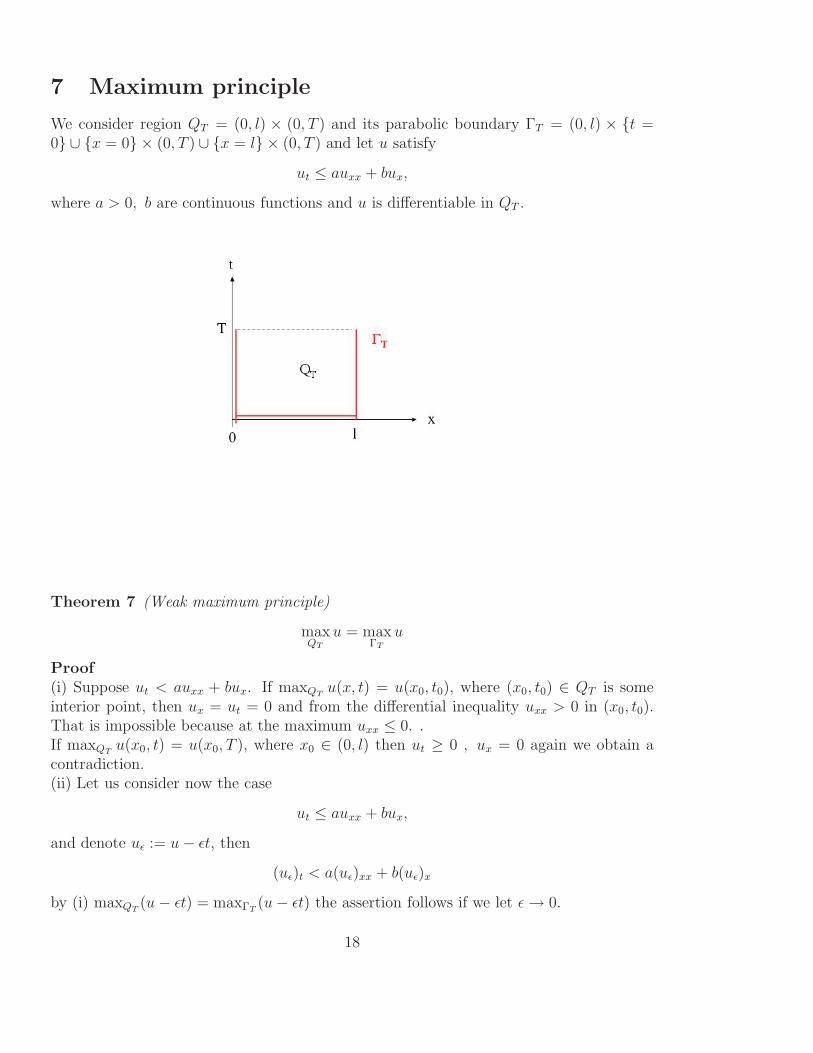
We consider region QT = (0, l) × (0, T ) and its parabolic boundary ΓT = (0, l) × {t =0} ∪ {x = 0} × (0, T ) ∪ {x = l} × (0, T ) and let u satisfy

ut ≤ auxx + bux,

where a > 0, b are continuous functions and u is differentiable in QT .

Theorem 7 (Weak maximum principle)

maxQT

u = maxΓT

u

Proof(i) Suppose ut < auxx + bux. If maxQT

u(x, t) = u(x0, t0), where (x0, t0) ∈ QT is someinterior point, then ux = ut = 0 and from the differential inequality uxx > 0 in (x0, t0).That is impossible because at the maximum uxx ≤ 0. .If maxQT

u(x0, t) = u(x0, T ), where x0 ∈ (0, l) then ut ≥ 0 , ux = 0 again we obtain acontradiction.(ii) Let us consider now the case

ut ≤ auxx + bux,

and denote uǫ := u − ǫt, then

(uǫ)t < a(uǫ)xx + b(uǫ)x

by (i) maxQT(u − ǫt) = maxΓT

(u − ǫt) the assertion follows if we let ǫ → 0.

18

Remark 1 Ifut ≤ auxx + bux,

then we cannot exclude from from the previous argument that the maximum lies both onΓT and in QT .

The next result clarifies the situation.

Theorem 8 (Strong maximum principle)If u attains its maximum at an interior point in QT , then u ≡ const.

7.1 Applications

7.1.1 Uniqueness

(A). We consider the following problem

(BVP1)

ut = auxx + bux + f(x, t) in (0, l) × R+

u(0, t) = ϕ1(t) , u(l, t) = ϕ2(t)

u(x, 0) = u0(x)

Theorem 9 (BVP1) has at most one solution.

ProofLet u1 and u2 be two solutions and d(x, t) := u1 − u2, then

dt = adxx + bdx in (0, l) × R+

and d(0, t) = d(l, t) = 0, d(x, 0) = 0. By the maximum principle

maxQT

d = minQT

d = 0

(B). The next problem contains an additional linear term

(BVP2)

ut = auxx + bux + c(x, t)u + f(x, t) in (0, l) × R+

u(0, t) = ϕ1(t) , u(l, t) = ϕ2(t)

u(x, 0) = u0(x)

Theorem 10 If |c(x, t)| ≤ c0 then there exist at most one solution to (BVP2).

ProofLet u1 and u2 be two solutions and d(x, t) := u1 − u2, then

dt = adxx + bdx + cd in (0, l) × R+

19

Consider e−c0td = σ then

σt = −c0e−c0td + e−c0tdt

= −c0σ + aσxx + bσx + cσ

= aσxx + bσx + (c − c0)σ

it is significant that c − c0 < 0. The claim σ cannot have negative minimum in QT ,however σ cannot reach its maximum in QT , consequently

maxQT

σ = minQT

σ = 0

(C). Let us consider

(BVP3)

ut = auxx + bux + c(x, t)u + f(x, t, u) in (0, l) × R+

u(0, t) = ϕ1(t) , u(l, t) = ϕ2(t)

u(x, 0) = u0(x)

Theorem 11 If f is differentiable in u and if |fu| is bounded then there is at most onesolution to (BVP3).

Proof Let ui, i = 1, 2 be two solutions. The difference d satisfies

dt = adxx + bdx + c(x, t)d + fu(x, t, u1 + θu2)d in (0, l) × R+

d(0, t) = 0 , d(l, t) = 0

d(x, 0) = 0.

If |f ′| is bounded then we can apply the previous result and conclude that d = 0.

Exercise Show that the theorem (10.5) remains valid for Lipschitz functions.

7.1.2 Estimates

Let

u t ≤ au xx + bu x + f in (0, l) × R+

u(0, t) ≤ 0 , u(l, t) ≤ 0

u(x, 0) ≤ u0(x)

Theorem 12 u is called a subsolution of (BVP3). Analogously we define a supersolutionu with reversed inequality signs .

Theorem 13 Let f be Lipschitz in u and let u, u be sub and super solutions. Then

u(x, t) ≤ u(x, t) ≤ u(x, t)

20

Example Consider the problem

ut = uxx + eu in (0, π) × R+, u(0, t) = u(π, t) = 0, u(x, 0) = u0(x).

If u0(x) ≥ 0, u = 0 is a sub solution. As a super solution we take the solution to theordinary differential equation u = eu, that is

u(t) = log

[1

e−max u0 − t

]

.

This super solution blows up at t∗ = e−max u0. It is interesting to observe that if u0 ≥ 0the solution of the reaction-diffusion problem blows up in finite time. A way to see it, isto multiply (test) the equation with sin x and to integrate. Then

∫ π

0

ut sin x dx = −∫ π

0

u sin x dx +

∫ π

0

eu sin x dx (7)

Jensen’s inequality implies∫ π

0

eu sin x dx ≥ 1

2e

∫ π0 u sinx dx.

Put

Φ(t) :=

∫ π

0

u sin x dx.

From (7) we deduce the differential inequality

Φ + Φ ≥ 1

2eΦ.

An elementary argument shows, that Φ cannot exist for all t. It tends to infinity at somefinite time t∗.

Exercise Prove the last statement.

ReferencesM. H. Protter, H. F. Weinberger, Maximum Principles in Differential Equations, PrenticeHall (1967).

8 Viscosity solutions

The existence theory for parabolic equations fails if instead of the diffusion operator △we have a(t, x)△ where a(t, x) vanishes somewhere.

Exampleut = x2uxx in R × R

+, u(x, 0) = |x|α, 0 < α < 1.

By means of separation of variables one obtains a formal solution of the form u(x, t) =|x|αeα(α−1)t. Notice that for the particular choice of α this is not a solution in the classical

21

sense because it is not differentiable in x = 0. The figure below shows the graph of u(x, t)for α = 1/2.

In order to include such less regular solutions, a different concept has been introducedwhich is described next.

Let us consider an equation of the general form

H(t, x, u, ut, ux, uxx) = 0, (x, t) ∈ QT . (8)

For simplicity we take x ∈ R. It satisfies the parabolicity condition, in the sense that ifM ≥ N then

H(t, x, u, p1, p2, M) ≤ H(t, x, u, p1, p2, N) ∀t, x, u, p1, p2.

Examples The reaction-diffusion equations satisfy the parabolicity condition.

22

Observation Let u ∈ C2 be a classical solution of (8) and let ϕ ∈ C2 be an arbitraryfunction of x and t. If (x0, t0) is a local maximum (minimum) of u − ϕ then ut(x0.t0) =ϕt(x0.t0), ux(x0.t0) = ϕx(x0.t0) and uxx(x0, t0) − ϕxx(x0.t0) ≤ 0, (≥ 0). Consequently bythe parabolicity condition

H(t0, x0, u(x0, t0), ϕt(x0, t0), ϕx(xo, t0), ϕxx(x0, t0)) ≤ 0 (resp. ≥ 0).

If those two inequalities are satisfied for all ϕ then u is a solution (choose ϕ = u)

Definition 14 (Continuous viscosity solution)If u is continuous and if for all ϕ ∈ C2 such that u−ϕ takes its maximum at (x0, t0) wehave

H(t0, x0, u(x0, t0), ϕt(x0, t0), ϕx(xo, t0), ϕxx(x0, t0)) ≤ 0

and if in addition, at a minimum point (x1, t1) of u − ϕ we have

H(t0, x0, u(x0, t0), ϕt(x0, t0), ϕx(xo, t0), ϕxx(x0, t0)) ≥ 0,

then u(x, t) is called a continuous viscosity solution.

If u is locally bounded instead of continuous it is called a discontinuous viscositysolution.

Exercise Prove that the solution in Example 2 is a viscosity solution.

Boundary value problems

Consider the parabolic boundary value problem

H(t, x, u, ut, ux, uxx) = 0 in QT , u = g on ΓT .

Here QT and ΓT have the same meaning as in Sec. 7. For a viscosity solution satisfyingthe boundary conditions, the following inequalities must be satisfied:

If the maximum (minimum) point (x0, t0), ((x1, t1) lies on the parabolic boundary γT

then

min{H(t, x, u, ϕt, ϕx, ϕxx), u − g|(x0,t0)} ≤ 0 ormax{H(t, x, u, ϕt, ϕx, ϕxx), u − g|(x1,t1)} ≥ 0.

ReferencesG. Barles, B. Perthame, Exit time problems in optimal control and the vanishing viscositymethod, SIAM J. Control Optim., 26 (1988), 1133-1148.

M. G. Crandall, L. C. Evans and P.-L. Lions, Some properties of viscosity solutions ofHamilton-Jacobi equations, TRAMS 282 (1984), 487-502.

23

9 Parabolic equations of more general type

Let us consider a domain (=open connected set) D in RN , x is a generic point and t > 0

stands for the time. Moreover we introduce a symmetric positive (N × N)-matrix A(aij = aji) such that

∑

aijξiξj ≥ λ|ξ|2, λ > 0,

and functions bi, i = 1 . . . N and c. Further we introduce the differential operator Lgiven by

Lu :=N∑

i,j=1

(aijuxj)xi

+N∑

i=1

biuxi+ cu

Definition 15 The equation

ut(x, t) = Lu + f in D × R+ (9)

is called a parabolic equation.

We distinguish between

• linear equations where

aij = aij(x, t)

bi = bi(x, t)

c = c(x, t)

f = f(x, t)

• nonlinear equations where

aij = aij(x, t, u,∇u)

bi = bi(x, t, u,∇u)

c = c(x, t, u,∇u)

f = f(x, t, u,∇u)

Examples of nonlinear equations: N = 1

1. ut = uxx + au(1 − u) Fisher’s equation

2. ut = ∂∂x

(umux) fast (m < 1)/slow (m > 1) diffusion

3. ut = uxx + uux Burger’s equation

And we consider two types of problems

24

• Cauchy problem. In this case D = RN

ut = Lu + f in RN × (0, T )

u(x, 0) = g(x) initial conditions (no boundary conditions)

• Boundary value problem. In this case D ⊂ RN

ut = Lu + f in D × (0, T )

(BC)

u = ϕ on ∂D × (0, T ) ( Dirichlet problem )

∂u

∂n= ϕ on ∂D × (0, T ) (Neumann problem )

(IC) u(x, 0) = g(x)

10 Weak solution

Let us consider the case N = 1 then we can rewrite equation (9) as

ut = (aux)x + bux + cu + f.

Let ϕ(x) be a smooth function then

l∫

0

utϕdx

︸ ︷︷ ︸

(ut,ϕ)

= −l∫

0

aϕxuxdx + ϕaux|l0 +

l∫

0

(bux + c)ϕdx +

l∫

0

fϕdx

︸ ︷︷ ︸

(f,ϕ)

(ut, ϕ) +

l∫

0

aϕxuxdx −l∫

0

(bux + c)ϕdx = ϕaux|l0 + (f, ϕ)

Suppose that ϕ(0) = ϕ(l) = 0. Then

(ut, ϕ) + a(u, ϕ) = (f, ϕ),

where a(u, ϕ) is a bilinear form. We want to interpret this equation in a Hilbert space.

10.1 Small excursion to functional analysis

Let us introduce some notation: H Hilbert space

( , ) scalar product‖ ‖ norm

25

Example

We consider the space L2 with a scalar product (f, g) =l∫

0

f · g dx and norm ‖f‖ =

(l∫

0

f 2dx

) 12

.

A linear functional A : H → R is a mapping such that

A(αf + βg) = αAf + βAg ∀α, β ∈ R.

A is bounded if ‖Ax‖‖x‖ ≤ ‖A‖ for any x ∈ H

Theorem 16 A linear operator is continuous if and only if it is bounded.

10.2 Generalized derivatives

Let us consider a set Γ = {ϕ(x) ∈ C∞0 (0, l)}. An example of an element in Γ is ϕ0(x) =

e− 1

(x−l/2)2−l2/4 .

Exercise: Prove that ϕ0 is infinitely often differentiable.

Definition 17 Let f , h be integrable. If

l∫

0

fϕ′dx = −l∫

0

hϕdx, ∀ϕ ∈ Γ

then h is a generalized derivative of f .

Generalized derivatives exist even if the function is not differentiable. Consider for in-stance the function f = |x| in (−1, 1). we have

∫ 1

−1

|x|φ′ dx = −∫ 0

−1

xφ′ dx +

∫ 1

0

xφ′ dx =

∫ 0

−1

φ dx +

∫ 1

0

φ dx.

The generalized derivative is therefore

f ′(x) =

{

−1 if x < 0

1 if x > 0

Consider the Heaviside function

f(x) =

{

0 in (0, l/2)

1 in (l/2, l).

Then ∫ l

0

fφ′ dx = φ(l/2) ∀φ ∈ Γ.

We cannot associate to f ′ a function h but a linear functional Tf ′(φ) = φ(l/2).

26

Definition 18 A distribution is a bounded linear functional T : Γ → R.

The Heaviside function possesses a derivative in the distributional sense.

Definition 19 The functional Tδyφ = φ(y) is called Dirac distribution.

ReferencesR. A. Adams, Sobolev Spaces, Academic Press (1975).

10.3 Sobolev spaces

Definition 20 The Sobolev space H1(0, l) is a Hilbert space consisting of the elements

{u : (0, l) → R, ux ∈ L2(0, l)}

and whose norm is defined as follows:

‖u‖H1 =

l∫

0

u2xdx +

l∫

0

u2dx

12

We say that un → u in H1 if ‖un − u‖H1 → 0. The definition above generalises immedi-ately to higher dimensions. The next Sobolev space takes into account that the functionsvanish in a generalised sense at the boundary.

Definition 21 H10(0, l) = {u ∈ H1(0, l) : ∃{un}∞n=1 ⊂ C∞

0 (0, l), u = limn→∞

un in H1}.

H1 and H10 are Hilbert spaces.

Exercises

1. Prove that a function in H1(0, l) is absolutely continuous.

2. Take D = B1(0) and f = |x|α. Prove that f belongs to H(B1(0)) if and only ifα < N−2

2.

10.4 Definition of weak solutions

Let us go back to the parabolic equation

(ut, ϕ) + a(u, ϕ) = (f, ϕ) ∀ϕ ∈ H10(0, l), (8.1)

and let us switch viewpoint. We interprete

u : [0, T ] → H10(0, l)

27

and denote by u′ the distributional derivative with respect to t.Then u is a weak solutionof (8.1) if

u ∈ L2(0, T ;H10)

andut = u′ ∈ L2(0, T ;H−1)

and (8.1) is satisfied. Here H−1 denotes the dual space of H10(0, l). More precisely

Definition 22 A function f belongs to the dual space, H−1 if there exists f 0 . . . fN in L2

such that

(f, v) = (f 0, v) +

N∑

i=1

(f i, vxi)

for any v ∈ H10(D). The H−1 is called a dual space to H1

0.

The space L2(0, T ; X), X Banach space, consists of elements u : (0, T ) → X such that

(∫ T

0

‖u‖2Xdt

) 12

< ∞.

11 Galerkin approximation

The Galerkin approximation provides a method to construct numerical solutions to theboundary value problem

ut = (aux)x + bux + c + f in (0, l) × R+, u(0, t) = u(l, t) = 0, u(x, 0) = u0(x).

It is an extension of the method of Fourier series considered in Sect. 6. We shall belooking for approximations to the weak solutions, Let {wk}∞k=1 be a basis of H1

0(0, l) suchthat the scalar product in L2(0, l) satisfies (wk, wj) = δkj. Set

um(x, t) =

m∑

k=1

dkm(t)wk(x)

um(x, 0) =

m∑

k=1

dkm(0)wk(x)

where dkm(0) = (u0, wk). We are looking for a solution of

(u′m, wj) + a(um, wj) = (f, wj) ∀j = 1 · · ·m.

This equation can be seen as the projection of the original problem into the space gener-ated by {wk}. The above equation leads to a first order system of differential equations

28

for the unknown dk(t), namely

dj′

m(t) +

m∑

k=1

dkm(t)a(wk, wj) = (f, wj)

djm(0) = (u0, wj)

j = 1 . . . k

We obtained the first order system of linear ODE’s with constant coefficients consequentlythere exists an unique solution.

Remark This method is also used to prove analytically the existence of solutions toparabolic problems. It applies to very general problems and to higher dimensions.

ReferencesO.A. Ladyzenskajia, N.N. Ural’tzeva, Linear and Quasilinear Equations of ParabolicType, Transl. Math, Monographs, 23, AMS, Providence R.I., (1968)A. Friedman, Partial Differential Equations of Parabolic Type, New York (1964).

29