
Introduction to Panel Data Analysis -...
155
Introduction to Panel Data Analysis Oliver Lipps / Ursina Kuhn Swiss Centre of Expertise in the Social Sciences (FORS) c/o University of Lausanne Lugano Summer School, 2016
Transcript of Introduction to Panel Data Analysis -...
Introduction to Panel Data Analysis
Oliver Lipps / Ursina Kuhn
Swiss Centre of Expertise in the Social Sciences (FORS) c/o University of Lausanne
Lugano Summer School, 2016
Introduction panel data, data management 1 Introducing panel data (OL) 2 The SHP (UK) 3 Data Management with Stata (UK) Regressions with panel data: basic 4 Regression refresher (UK) 5 Causality (OL) 6 Fixed effects models (OL) 7 Random Effects (random intercept) models (OL) 8 Nonlinear regression (UK) Additional topics 9 Missing data (OL), 10 Random Slope models (OL) 11 Dynamic models (UK)
1 - 2

Organisation Morning (8.30-12.30, break ca 10.30-10.45) - Classroom - Theory and application examples Lunch Break 12.30-13.30 Afternoon (13.30-17.00, break ca. 15.30-15.45) Hands-on; aim: apply what we discussed in the morning
– Data management and descriptive analysis with panel data – Regression models with panel data
Prepared data sets and exercises or work with your own data Discussion of individual questions whenever possible
1 - 3

1 - 4
Purpose of this Summer School
To introduce basic methods of panel data analysis: • Emphasis on causal effects (within variation) but also
descriptive methods (OLS) • Less emphasis on complex methods (dynamic models,
instruments) • Practical implementation with Stata, do-files (and data) • Data preparation
• Presenting and interpreting results • Graphical display of regression results

1 - 5
Surveys over time: repeated cross-sections vs. panels
• Cross-Sectional Survey: conducted at one or several points in time (“rounds”) using different respondents in each round
• Panel Survey: conducted at several points in time
(“waves”) using the same sample respondents over waves
→ panel data mostly from prospective (panel) surveys → also: from retrospective (“biographical”) survey

1 - 6
Panel Surveys: to distinguish
Length and sample size: • Time Series: N small (mostly=1), T large (T→∞) → time series models (finance, macro-economics, demography, …)
• Panel Surveys: N large, T small (N→∞) → social science panel surveys (sociology, microeconomics, …)
Sample • General population:
- rotating: only few (pre-defined number) waves per individual (in CH: SILC, LFS)
- indefinitely long (in CH: SHP)
• Special population: - e.g., age/birth cohorts (in CH e.g.: TREE, SHARE, COCON)
representative for population of special age group / birth years
1 - 7
Panel surveys increasingly important
Changing focus in social sciences → Life course research: individual trajectories (e.g., growth
curves, transitions into and out of states) → Identify “causal effects” (unbiased estimates) rather than
correlations → Large investments in social science panel surveys, high
data quality! Analysis potential of panel data
- close to experimental design: before and after studies of treated
- Control of unobserved time-invariant individual characteristics (FE Models)
1 - 8
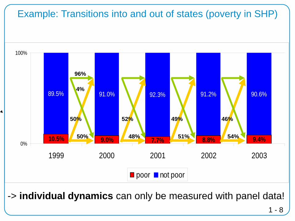
Example: Transitions into and out of states (poverty in SHP)
-> individual dynamics can only be measured with panel data!
10.5% 9.0% 7.7% 8.8% 9.4%
89.5% 91.0% 92.3% 91.2% 90.6%
0%
100%
1999 2000 2001 2002 2003
poor not poor
54%
46%
51%
49%
48%
52%
50%
50%
96%
4%

1 - 9
Identification of age, time, and (birth) cohort effects
Fundamental relationship: ait = t – ci (eg 30 = 2014 - 1984) • Effects from “formative” years (childhood, youth) -> cohort effect
(e.g. taste in music ) • Time may affect behavior -> time effect (e.g. computer
performance, economic cycle) • Behavior may change over the life cycle-> age effect (e.g. health)
• In a cross-section, t is constant → age and cohort collinear (only joint effect estimable) • In a cohort study, cohort is constant → age and time collinear (only joint effect estimable) • In a panel, Ait, t, and ci collinear. → only two of the three effects can be estimated → we can use (t,ci), (Ait,ci), or (Ait,t), but not all three
1 - 10
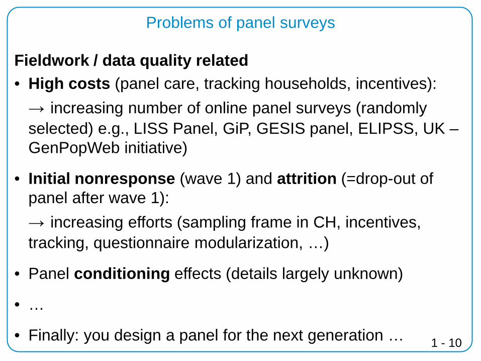
Problems of panel surveys
Fieldwork / data quality related • High costs (panel care, tracking households, incentives):
→ increasing number of online panel surveys (randomly selected) e.g., LISS Panel, GiP, GESIS panel, ELIPSS, UK – GenPopWeb initiative)
• Initial nonresponse (wave 1) and attrition (=drop-out of panel after wave 1): → increasing efforts (sampling frame in CH, incentives, tracking, questionnaire modularization, …)
• Panel conditioning effects (details largely unknown)
• …
• Finally: you design a panel for the next generation …

2 Introducing the Swiss Household Panel (SHP)

2-2
Swiss Household Panel: overview
• Primary goal: observe social change and changing life conditions in Switzerland
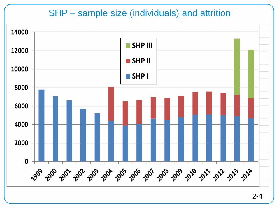
• First wave in 1999, more than 5,000 households. Refreshment samples in 2004, more than 2,500 households, several new questions, and in 2013 (more than 4,500 households, full questionnaire from 2014 on (2013: biographical questionnaire)
• Run by FORS (Swiss Centre of Expertise in the Social Sciences ), c/o University of Lausanne
• Financed by Swiss National Science Foundation

2-3
SHP – sample and methods
• Representative of the Swiss residential population
• Each individual surveyed every year (Sept.-Jan.)
• All household members from 14 years on surveyed (proxy questionnaire if child or unable)
• Telephone interviews (central CATI), languages D/F/I
• Metadata: biography, interviewers, call data
Following rules:
• OSM followed if moving, from 2007 on all individuals
• All new household entrants surveyed
2-4
SHP – sample size (individuals) and attrition
0
2000
4000
6000
8000
10000
12000
14000
SHP III
SHP II
SHP I
2-5
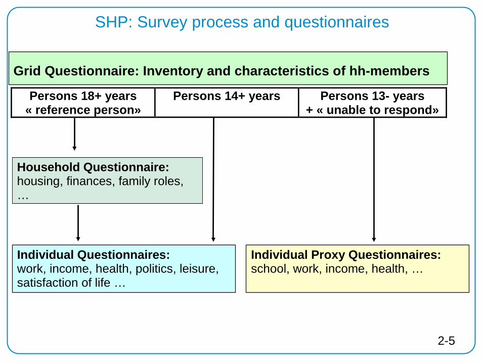
Persons 18+ years « reference person»
Persons 14+ years
Persons 13- years + « unable to respond»
Household Questionnaire: housing, finances, family roles, …
Grid Questionnaire: Inventory and characteristics of hh-members
Individual Questionnaires: work, income, health, politics, leisure, satisfaction of life …
Individual Proxy Questionnaires: school, work, income, health, …
SHP: Survey process and questionnaires

2-6
SHP: Questionnaire Content
• Social structure: socio-demography, socio-ecomomy, work, education, social origin, income, housing, religion
• Life events: marriages, births, deaths, deceases, accidents, conflicts with close persons, etc.
• Politics : attitudes, participation, party preference)
• Social participation: culture, social network, leisure
• Perception and values: trust, confidence, gender • Satisfaction: different satisfaction issues
• Health: physical and mental health self-evaluation, chronic problems
• Psychological scales

2-7
SHP Questionnaire: Rotation modules
Module 2010 2011 2012 2013 2014 2015 2016 2017 2018 2019 2020
Social network
X X X X
Religion X X X
Social participation
X X X X
Politics X X X X
Leisure X X X X
Psychologi-cal Scales
X X X
2-8
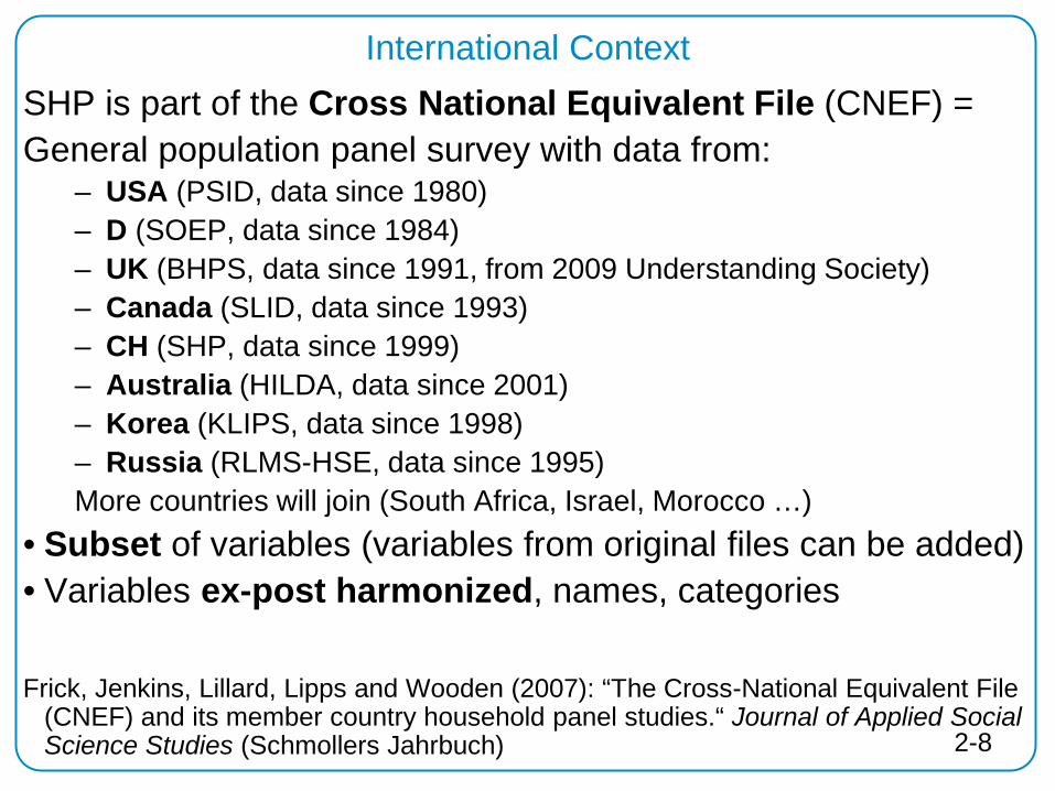
International Context SHP is part of the Cross National Equivalent File (CNEF) = General population panel survey with data from:
– USA (PSID, data since 1980) – D (SOEP, data since 1984) – UK (BHPS, data since 1991, from 2009 Understanding Society) – Canada (SLID, data since 1993) – CH (SHP, data since 1999) – Australia (HILDA, data since 2001) – Korea (KLIPS, data since 1998) – Russia (RLMS-HSE, data since 1995) More countries will join (South Africa, Israel, Morocco …)
• Subset of variables (variables from original files can be added) • Variables ex-post harmonized, names, categories
Frick, Jenkins, Lillard, Lipps and Wooden (2007): “The Cross-National Equivalent File (CNEF) and its member country household panel studies.“ Journal of Applied Social Science Studies (Schmollers Jahrbuch)
2-9
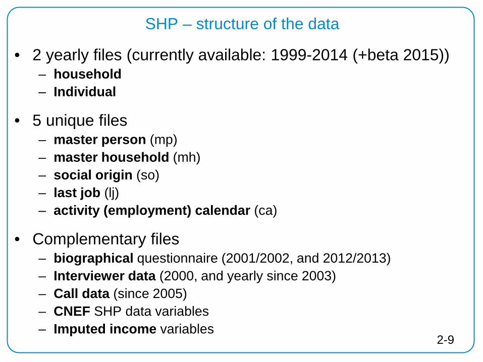
SHP – structure of the data
• 2 yearly files (currently available: 1999-2014 (+beta 2015)) – household – Individual
• 5 unique files – master person (mp) – master household (mh) – social origin (so) – last job (lj) – activity (employment) calendar (ca)
• Complementary files – biographical questionnaire (2001/2002, and 2012/2013) – Interviewer data (2000, and yearly since 2003) – Call data (since 2005) – CNEF SHP data variables – Imputed income variables
2-10
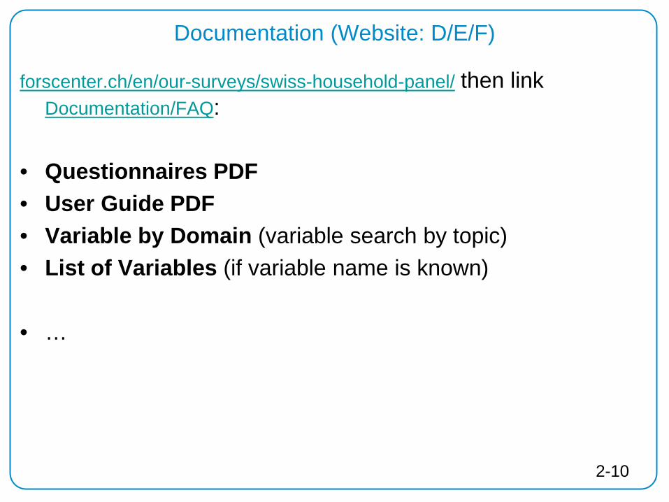
Documentation (Website: D/E/F)
forscenter.ch/en/our-surveys/swiss-household-panel/ then link Documentation/FAQ:
• Questionnaires PDF • User Guide PDF • Variable by Domain (variable search by topic) • List of Variables (if variable name is known) • …
2-11
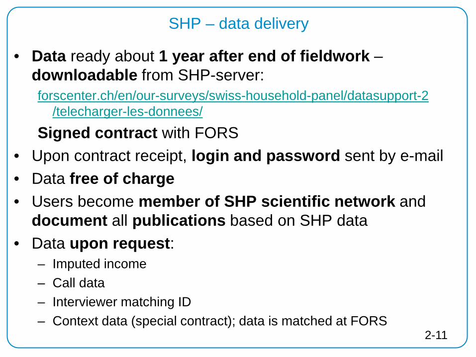
SHP – data delivery
• Data ready about 1 year after end of fieldwork – downloadable from SHP-server: forscenter.ch/en/our-surveys/swiss-household-panel/datasupport-2
/telecharger-les-donnees/
Signed contract with FORS • Upon contract receipt, login and password sent by e-mail • Data free of charge • Users become member of SHP scientific network and
document all publications based on SHP data • Data upon request:
– Imputed income – Call data – Interviewer matching ID – Context data (special contract); data is matched at FORS
3
Stata and panel data
3_2
Why Stata?
Capabilities — Data management — Broad range of statistics
– Powerful for panel data! – Many commands ready for analysis – User-written extensions
Beginners and experienced users — Beginners: analysis through menus (point and click) — Advanced users: good programmable capacities
3_3
Starting with Stata
Basics — Look at the data, check variables — Descriptive statistics — Regression analysis
→ Handout Stata basics Working with panel data — Merge — Creating « long files » — Working with the long file — Add information from other household members
→ Handout Stata SHP data management (includes Syntax examples, exercises)
3_4
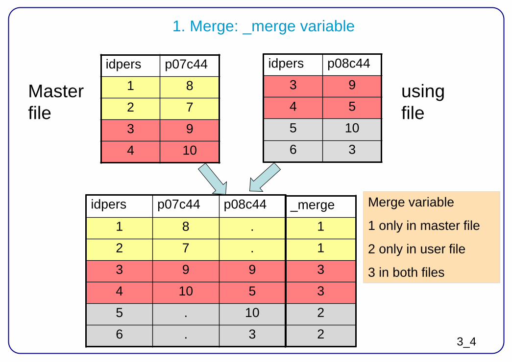
1. Merge: _merge variable
idpers p07c44 1 8 2 7 3 9 4 10
idpers p08c44 3 9 4 5 5 10 6 3
idpers p07c44 p08c44
1 8 . 2 7 . 3 9 9 4 10 5 5 . 10 6 . 3
Master file
using file
_merge 1 1 3 3 2 2
Merge variable
1 only in master file
2 only in user file
3 in both files

3_5
Merge: identifier
idpers p07c44
1 8
2 7
3 9
4 10
idpers p08c44 3 9 4 5 5 10 6 3
idpers p07c44 p08c44
1 8 . 2 7 . 3 9 9 4 10 5 5 . 10 6 . 3
Master file
using file
_merge 1 1 3 3 2 2
3_6
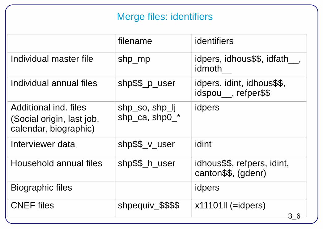
Merge files: identifiers
filename identifiers
Individual master file shp_mp idpers, idhous$$, idfath__, idmoth__
Individual annual files shp$$_p_user idpers, idint, idhous$$, idspou__, refper$$
Additional ind. files (Social origin, last job, calendar, biographic)
shp_so, shp_lj shp_ca, shp0_*
idpers
Interviewer data shp$$_v_user idint
Household annual files shp$$_h_user idhous$$, refpers, idint, canton$$, (gdenr)
Biographic files idpers
CNEF files shpequiv_$$$$ x11101ll (=idpers)
3_7
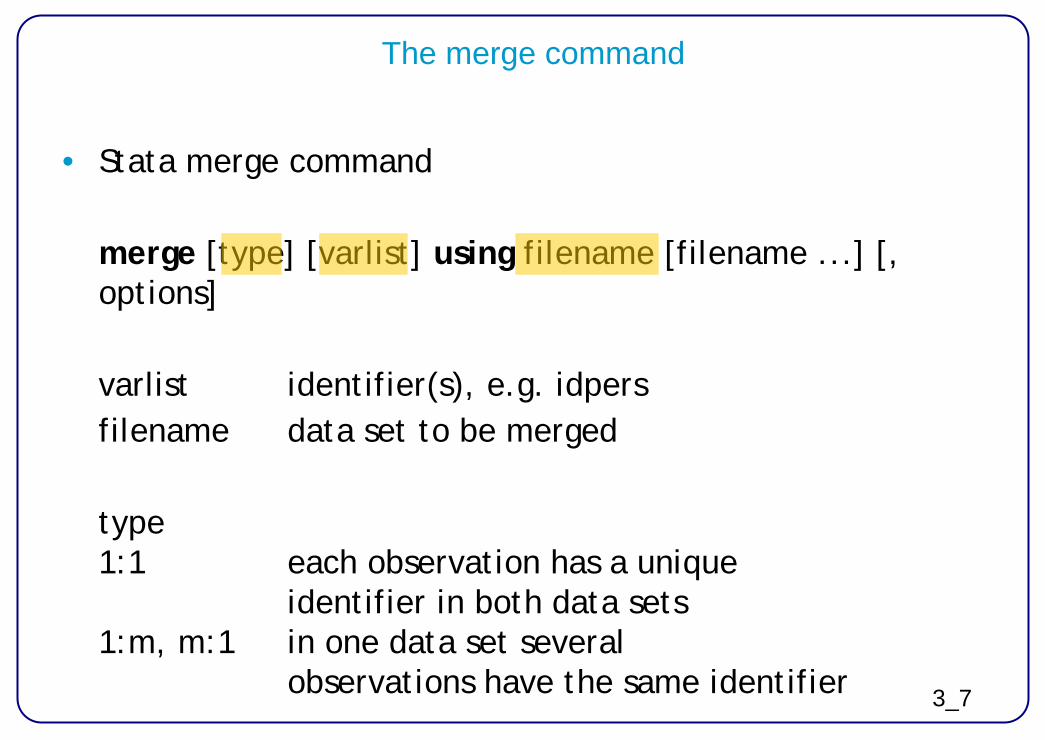
The merge command
• Stata merge command merge [type] [varlist] using filename [filename ...] [,
options] varlist identifier(s), e.g. idpers filename data set to be merged type
1:1 each observation has a unique identifier in both data sets 1:m, m:1 in one data set several observations have the same identifier

3_8
1:1 merge individual files
2 annual individual files use shp08_p_user, clear merge 1:1 idpers using shp00_p_user _merge | Freq. Percent Cum. ------------+----------------------------------- 1 | 5,845 34.93 34.93 2 | 5,056 30.21 65.14 3 | 5,833 34.86 100.00 ------------+----------------------------------- Total | 16,734 100.00
3_9
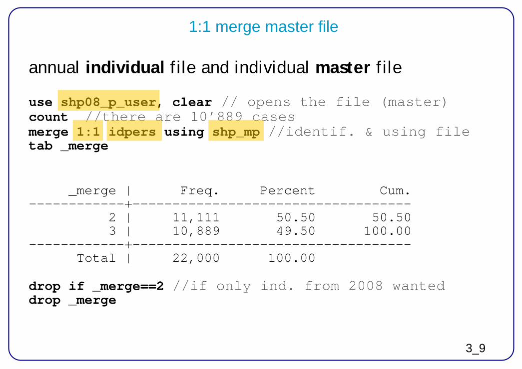
1:1 merge master file
annual individual file and individual master file use shp08_p_user, clear // opens the file (master) count //there are 10’889 cases merge 1:1 idpers using shp_mp //identif. & using file tab _merge
_merge | Freq. Percent Cum. ------------+----------------------------------- 2 | 11,111 50.50 50.50 3 | 10,889 49.50 100.00 ------------+----------------------------------- Total | 22,000 100.00 drop if _merge==2 //if only ind. from 2008 wanted drop _merge
3_10
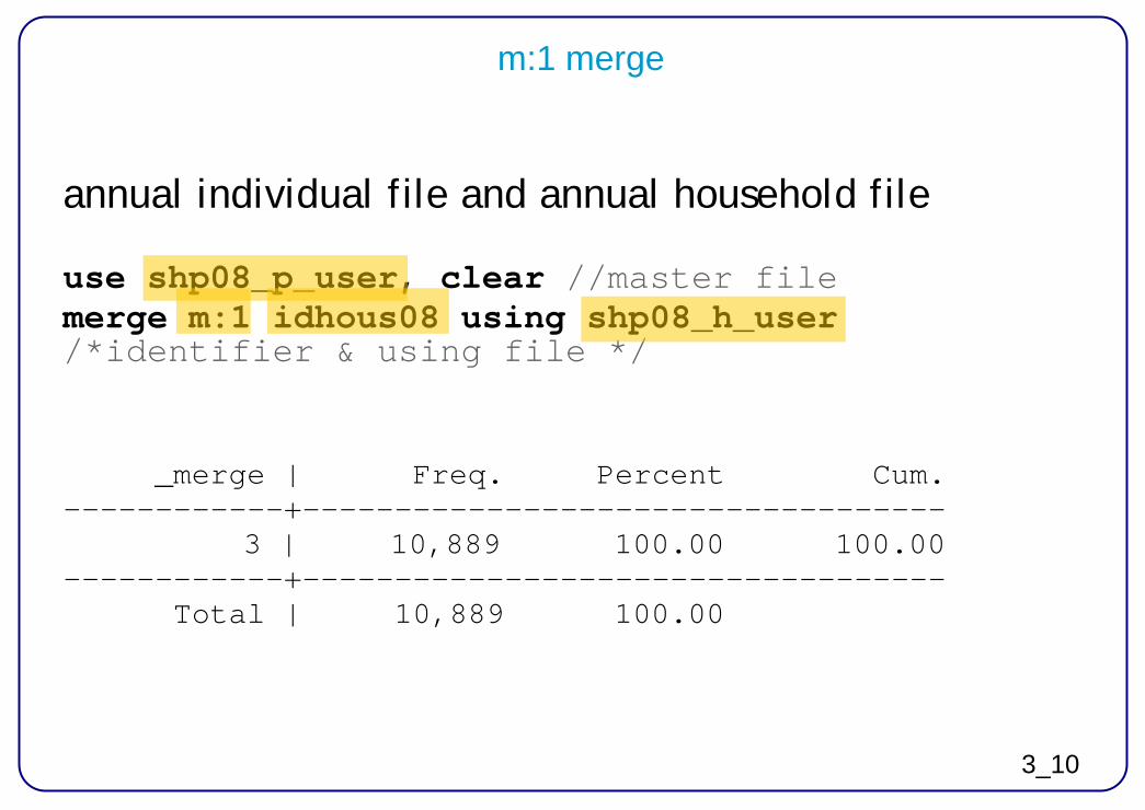
m:1 merge
annual individual file and annual household file
use shp08_p_user, clear //master file merge m:1 idhous08 using shp08_h_user /*identifier & using file */ _merge | Freq. Percent Cum. ------------+----------------------------------- 3 | 10,889 100.00 100.00 ------------+----------------------------------- Total | 10,889 100.00
3_11
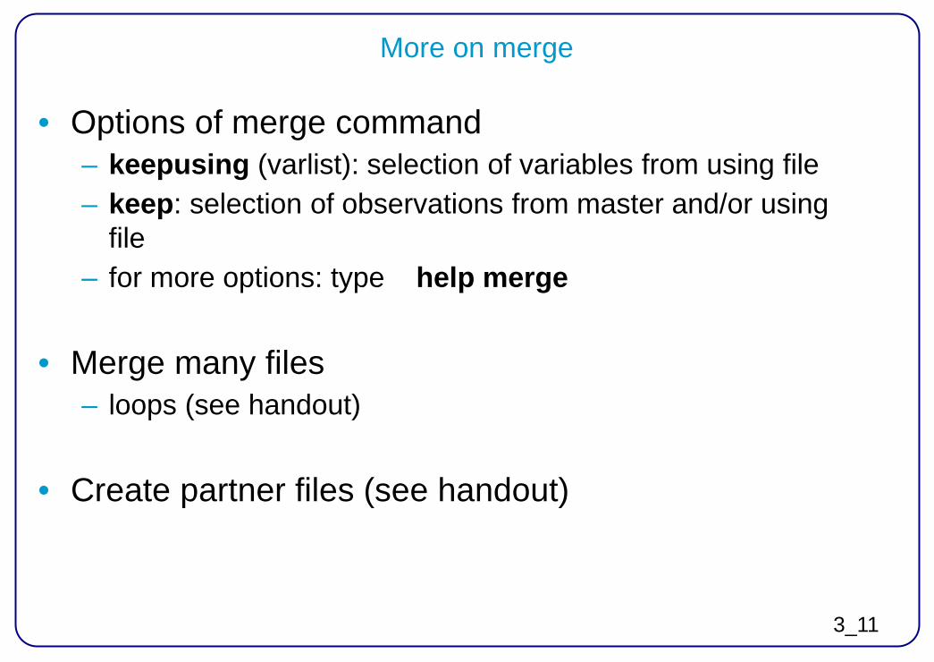
More on merge
• Options of merge command – keepusing (varlist): selection of variables from using file – keep: selection of observations from master and/or using
file – for more options: type help merge
• Merge many files
– loops (see handout)
• Create partner files (see handout)
3_12
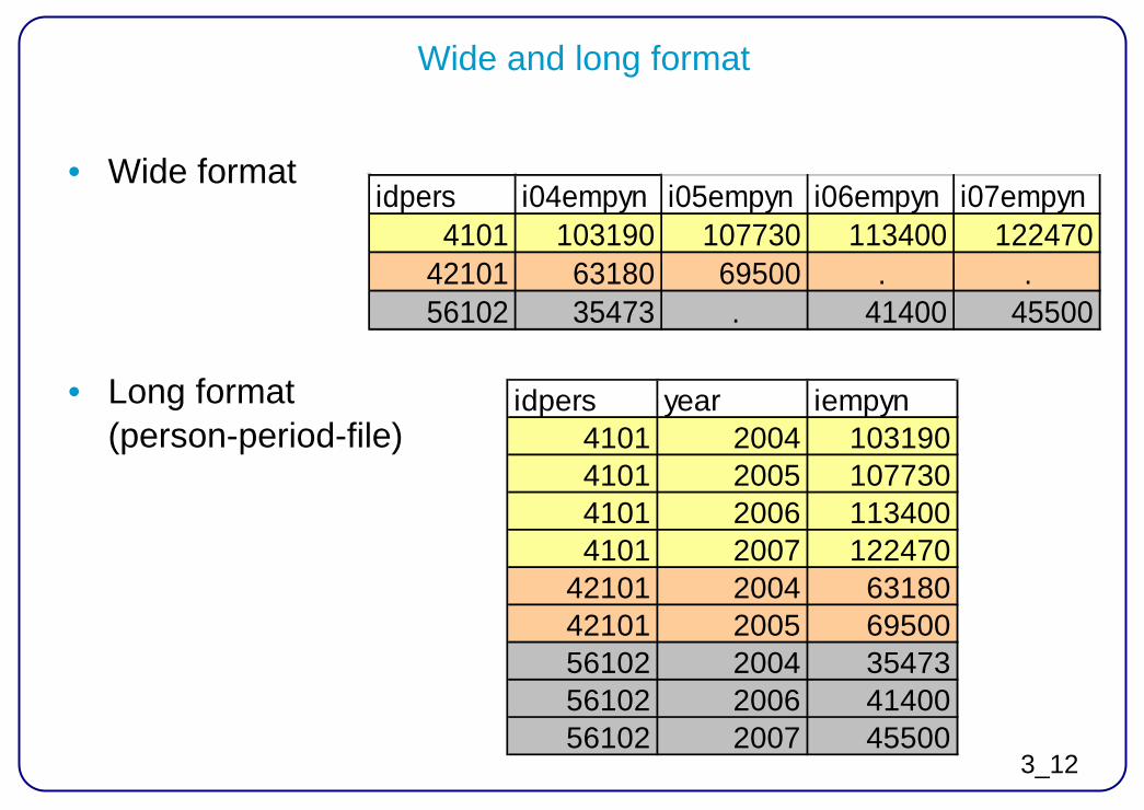
Wide and long format
• Wide format
• Long format (person-period-file)
idpers year iempyn4101 2004 1031904101 2005 1077304101 2006 1134004101 2007 122470
42101 2004 6318042101 2005 6950056102 2004 3547356102 2006 4140056102 2007 45500
idpers i04empyn i05empyn i06empyn i07empyn4101 103190 107730 113400 122470
42101 63180 69500 . .56102 35473 . 41400 45500
3_13
Use of long data format
• All panel applications: xt commands – descriptives – panel data models
• fixed effects models, random effects, multilevel • discrete time event-history analysis
• declare panel structure
panel identifier, time identifier xtset idpers wave
3_14
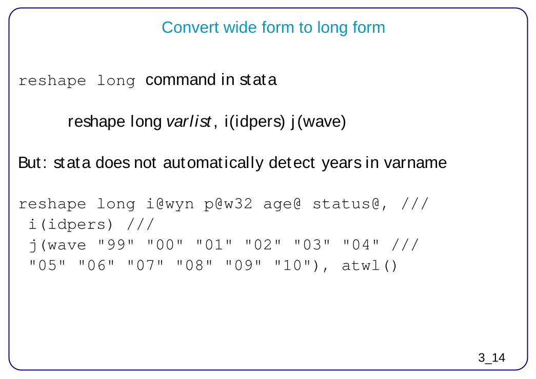
Convert wide form to long form
reshape long command in stata reshape long varlist, i(idpers) j(wave) But: stata does not automatically detect years in varname
reshape long i@wyn p@w32 age@ status@, /// i(idpers) /// j(wave "99" "00" "01" "02" "03" "04" /// "05" "06" "07" "08" "09" "10"), atwl()
3_15
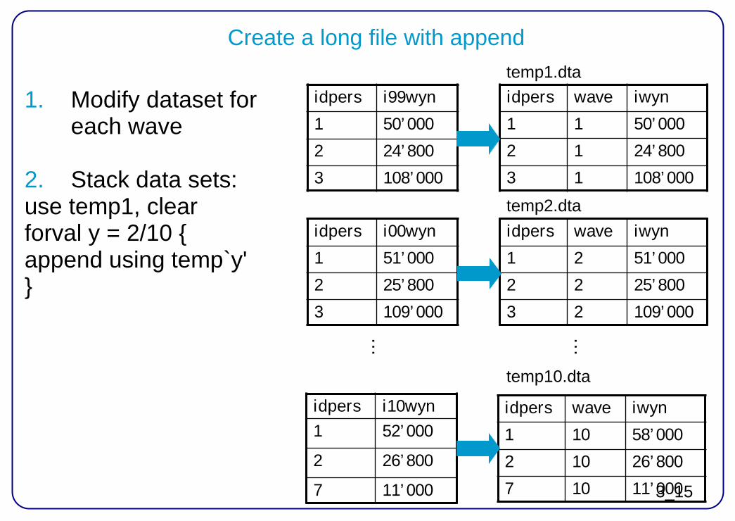
Create a long file with append
1. Modify dataset for each wave 2. Stack data sets: use temp1, clear forval y = 2/10 { append using temp`y' }
idpers wave iwyn
1 1 50’000
2 1 24’800
3 1 108’000
idpers i99wyn
1 50’000
2 24’800
3 108’000
temp2.dta idpers i00wyn
1 51’000
2 25’800
3 109’000
idpers i10wyn 1 52’000
2 26’800
7 11’000
idpers wave iwyn
1 2 51’000
2 2 25’800
3 2 109’000
idpers wave iwyn
1 10 58’000
2 10 26’800
7 10 11’000
…
…
temp10.dta
temp1.dta
3_16
Work with time lags
— If data in long format and defined as panel data (xtset) — l. indicates time lag — f. indicates time lead
— Example:
social class of last job (see handout) life events
3_17
Missing data in the SHP
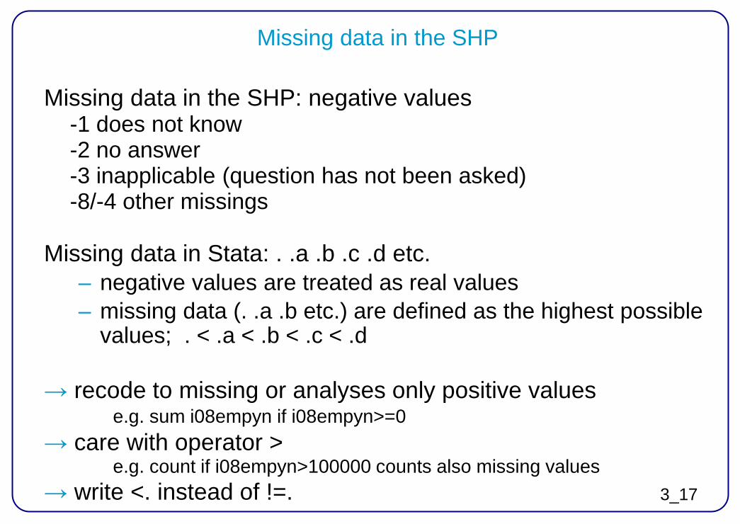
Missing data in the SHP: negative values -1 does not know -2 no answer -3 inapplicable (question has not been asked) -8/-4 other missings Missing data in Stata: . .a .b .c .d etc.
– negative values are treated as real values – missing data (. .a .b etc.) are defined as the highest possible
values; . < .a < .b < .c < .d
→ recode to missing or analyses only positive values e.g. sum i08empyn if i08empyn>=0
→ care with operator > e.g. count if i08empyn>100000 counts also missing values
→ write <. instead of !=.

3_18
Longitudinal data analysis with Stata
xt commands: descriptive statistics
– xtdescribe – xtsum, xttab, xttrans
regression analysis
– Random Intercept: xtreg, xtgls, xtlogit, xtpoisson, xtcloglog
– Random Slope: mixed, melogit, …
diagrams: xtline
3_19
Descriptive analysis
• Get to know the data • Usually: similar findings to complicated models • Visualisation • Accessible results to a wider public • Assumptions more explicit than in complicated models

3_20
Example: variability of party preferences
Kuhn (2009), Swiss Political Science Review 15(3): 463-494
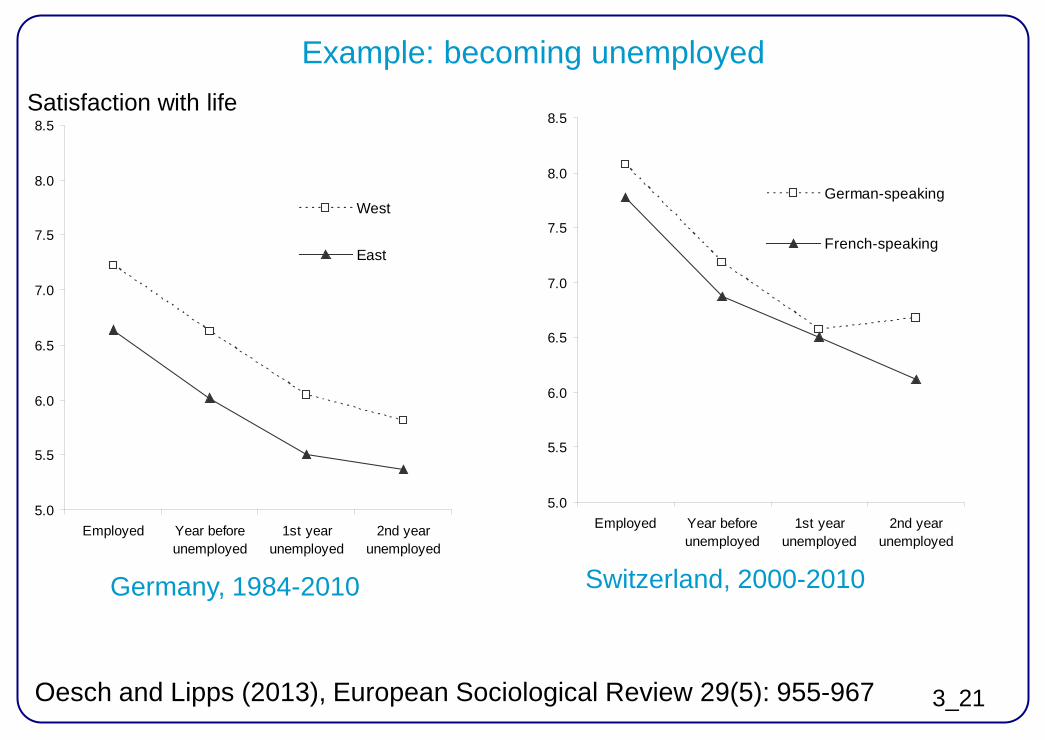
3_21 Oesch and Lipps (2013), European Sociological Review 29(5): 955-967
5.0
5.5
6.0
6.5
7.0
7.5
8.0
8.5
Employed Year beforeunemployed
1st yearunemployed
2nd yearunemployed
West
East
5.0
5.5
6.0
6.5
7.0
7.5
8.0
8.5
Employed Year beforeunemployed
1st yearunemployed
2nd yearunemployed
German-speaking
French-speaking
Germany, 1984-2010 Switzerland, 2000-2010
Example: becoming unemployed Satisfaction with life

3_22
Example: Income mobility
Grabka and Kuhn (2012), Swiss Journal of Sociology 38(2): 311–334
Switzerland Low income 2009
Middle income 2009
High income 2009
Total
Low income 2005 56.2 % 40.8 % 3.1 % 100 %
Middle income 2005 13.5 % 75.8 % 10.8 % 100 %
High income 2005 4.4 % 34.4 % 61.1 % 100 %
Germany Low income 2009
Middle income 2009
High income 2009
Total
Low income 2005 61.7 % 36.4 % 1.9 % 100 %
Middle income 2005 12.4 % 78.4 % 9.2 % 100 %
High income 2005 2.6 % 29.6 % 67.8 % 100 %

4_1
4 Linear regression (Refresher course)

4_2
Aim and content
Refresher course on linear regression — What is a regression? — How to obtain regression coefficients? — How to interpret regression coefficients? — Inference from sample to population of interest (significance
tests)
— Assumptions of linear regression — Consequences when assumptions are violated
4_3
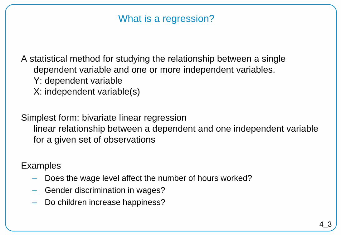
What is a regression?
A statistical method for studying the relationship between a single dependent variable and one or more independent variables. Y: dependent variable X: independent variable(s)
Simplest form: bivariate linear regression
linear relationship between a dependent and one independent variable for a given set of observations
Examples
‒ Does the wage level affect the number of hours worked? ‒ Gender discrimination in wages? ‒ Do children increase happiness?

4_4
20000
60000
40000
80000
100000
120000ye
arly
inco
me
from
em
ploy
men
t
0 10 20 30 40 50number of years spent in paid work
We start with a “scatter plot” of observations

4_5
Regression line: ŷi = a + bxi = 51375 + 693 *xi
20000
60000
40000
80000
100000
120000ye
arly
inco
me
from
em
ploy
men
t
0 10 20 30 40 50number of years spent in paid work
a
1 unit x b

4_6
Regression line: ŷi = a + b*xi = 51375 + 693*xi Estimated regression equation: yi = a + b xi + ei
20000
60000
40000
80000
100000
120000 ye
arly
inco
me
from
em
ploy
men
t
0 10 20 30 40 50 number of years spent in paid work
4_7
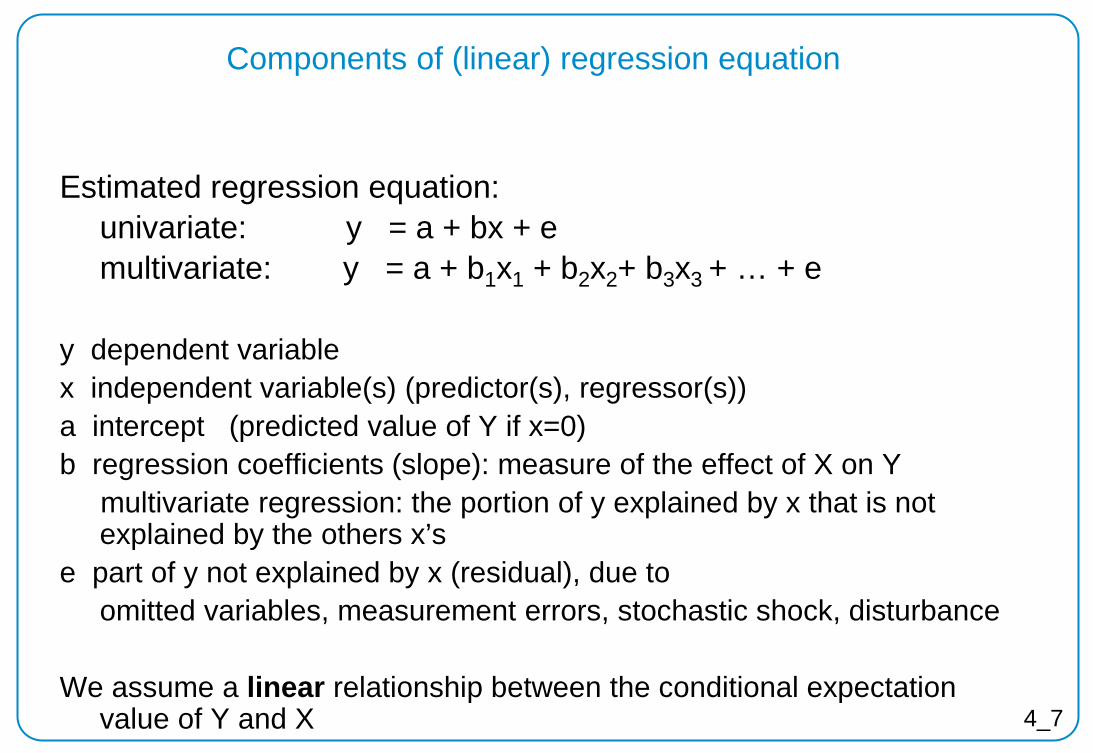
Components of (linear) regression equation
Estimated regression equation: univariate: y = a + bx + e
multivariate: y = a + b1x1 + b2x2+ b3x3 + … + e y dependent variable x independent variable(s) (predictor(s), regressor(s)) a intercept (predicted value of Y if x=0) b regression coefficients (slope): measure of the effect of X on Y multivariate regression: the portion of y explained by x that is not
explained by the others x’s e part of y not explained by x (residual), due to omitted variables, measurement errors, stochastic shock, disturbance We assume a linear relationship between the conditional expectation
value of Y and X
4_8
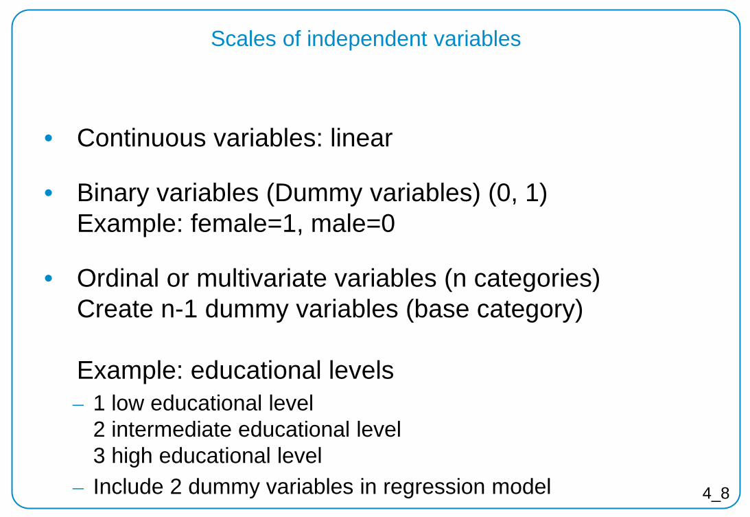
Scales of independent variables
• Continuous variables: linear
• Binary variables (Dummy variables) (0, 1) Example: female=1, male=0
• Ordinal or multivariate variables (n categories) Create n-1 dummy variables (base category) Example: educational levels – 1 low educational level
2 intermediate educational level 3 high educational level
– Include 2 dummy variables in regression model

distribution (Y|X)
Regression – graphical interpretation
distribution (Y|X)
4_9
4_10
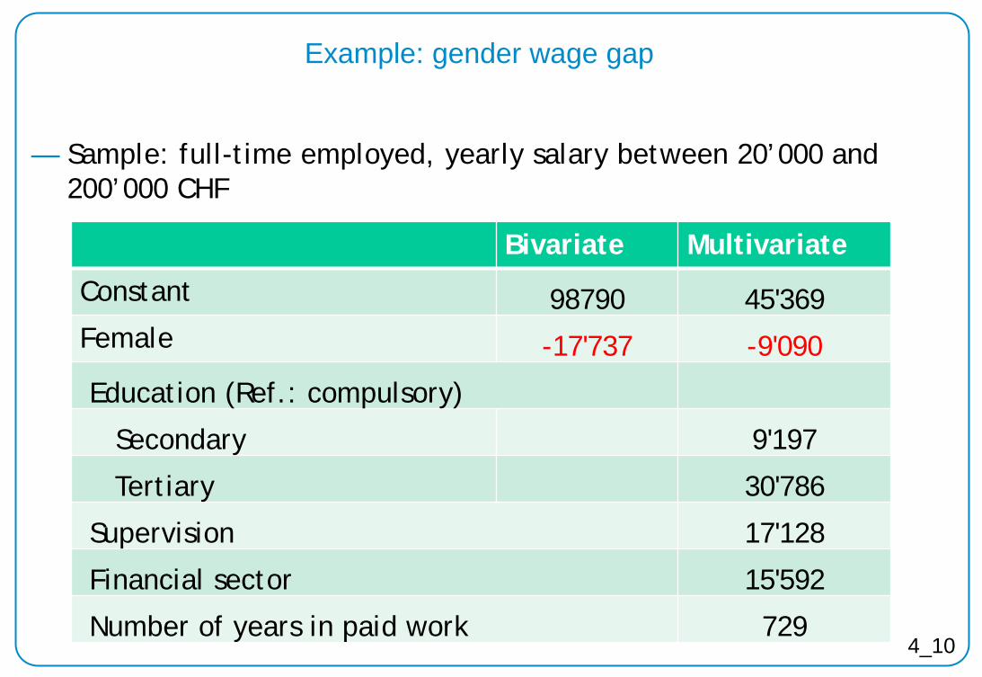
Example: gender wage gap
— Sample: full-time employed, yearly salary between 20’000 and 200’000 CHF
Bivariate Multivariate
Constant 98790 45'369 Female -17'737 -9'090
Education (Ref.: compulsory)
Secondary 9'197
Tertiary 30'786
Supervision 17'128
Financial sector 15'592
Number of years in paid work 729
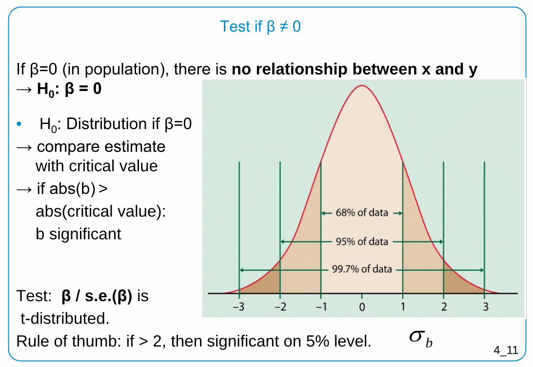
Test if β ≠ 0
If β=0 (in population), there is no relationship between x and y → H0: β = 0
• H0: Distribution if β=0 → compare estimate
with critical value → if abs(b) > abs(critical value): b significant
Test: β / s.e.(β) is t-distributed. Rule of thumb: if > 2, then significant on 5% level.
b
bv a l utbσ
=−=s t a n d
bσ 4_11
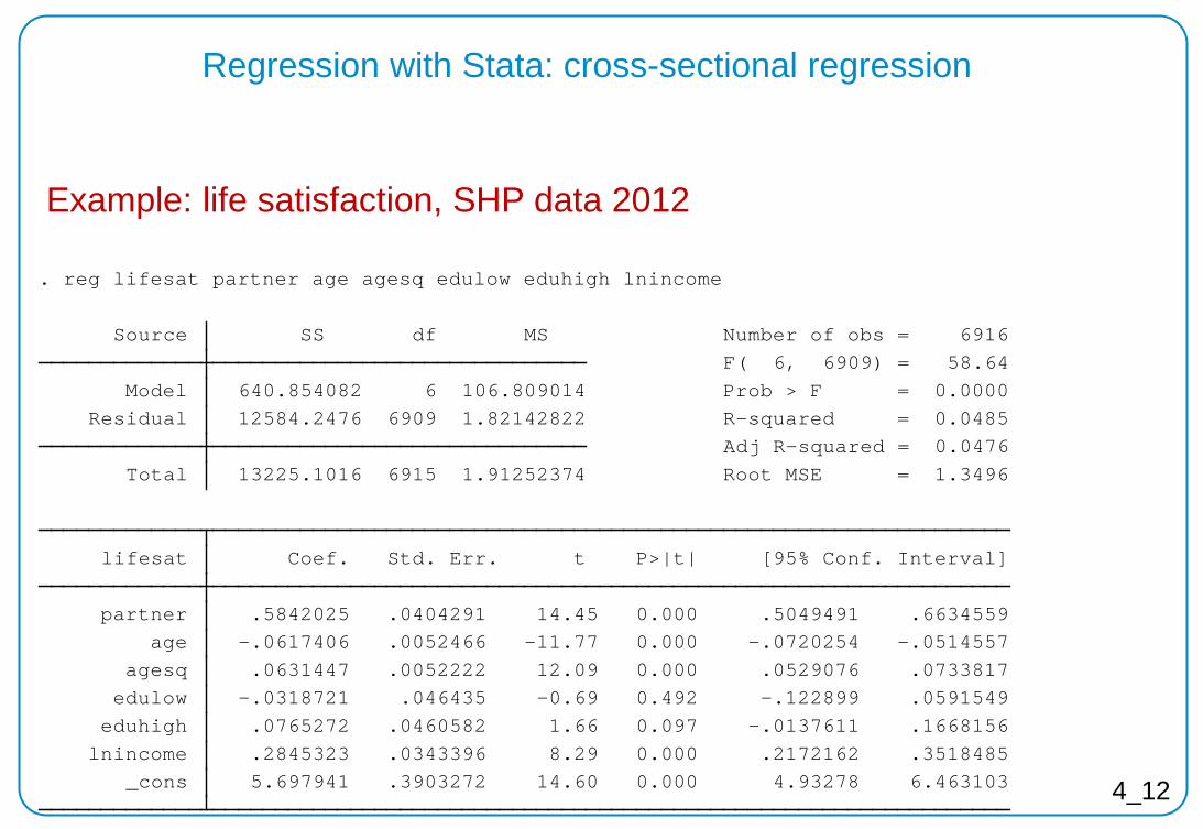
Regression with Stata: cross-sectional regression
Example: life satisfaction, SHP data 2012
_cons 5.697941 .3903272 14.60 0.000 4.93278 6.463103 lnincome .2845323 .0343396 8.29 0.000 .2172162 .3518485 eduhigh .0765272 .0460582 1.66 0.097 -.0137611 .1668156 edulow -.0318721 .046435 -0.69 0.492 -.122899 .0591549 agesq .0631447 .0052222 12.09 0.000 .0529076 .0733817 age -.0617406 .0052466 -11.77 0.000 -.0720254 -.0514557 partner .5842025 .0404291 14.45 0.000 .5049491 .6634559 lifesat Coef. Std. Err. t P>|t| [95% Conf. Interval]
Total 13225.1016 6915 1.91252374 Root MSE = 1.3496 Adj R-squared = 0.0476 Residual 12584.2476 6909 1.82142822 R-squared = 0.0485 Model 640.854082 6 106.809014 Prob > F = 0.0000 F( 6, 6909) = 58.64 Source SS df MS Number of obs = 6916
. reg lifesat partner age agesq edulow eduhigh lnincome
4_12
4_13
E(β)
σ β
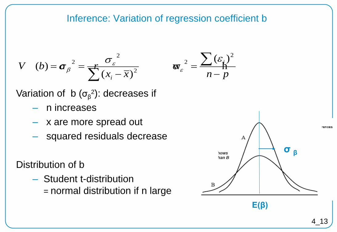
Inference: Variation of regression coefficient b
pnxxbV a r i
i −=
−== ∑∑
22
2
22 )(
w h)(
)(ε
σσσ εε
β
Variation of b (σβ2): decreases if
‒ n increases ‒ x are more spread out ‒ squared residuals decrease
Distribution of b
‒ Student t-distribution = normal distribution if n large
4_14
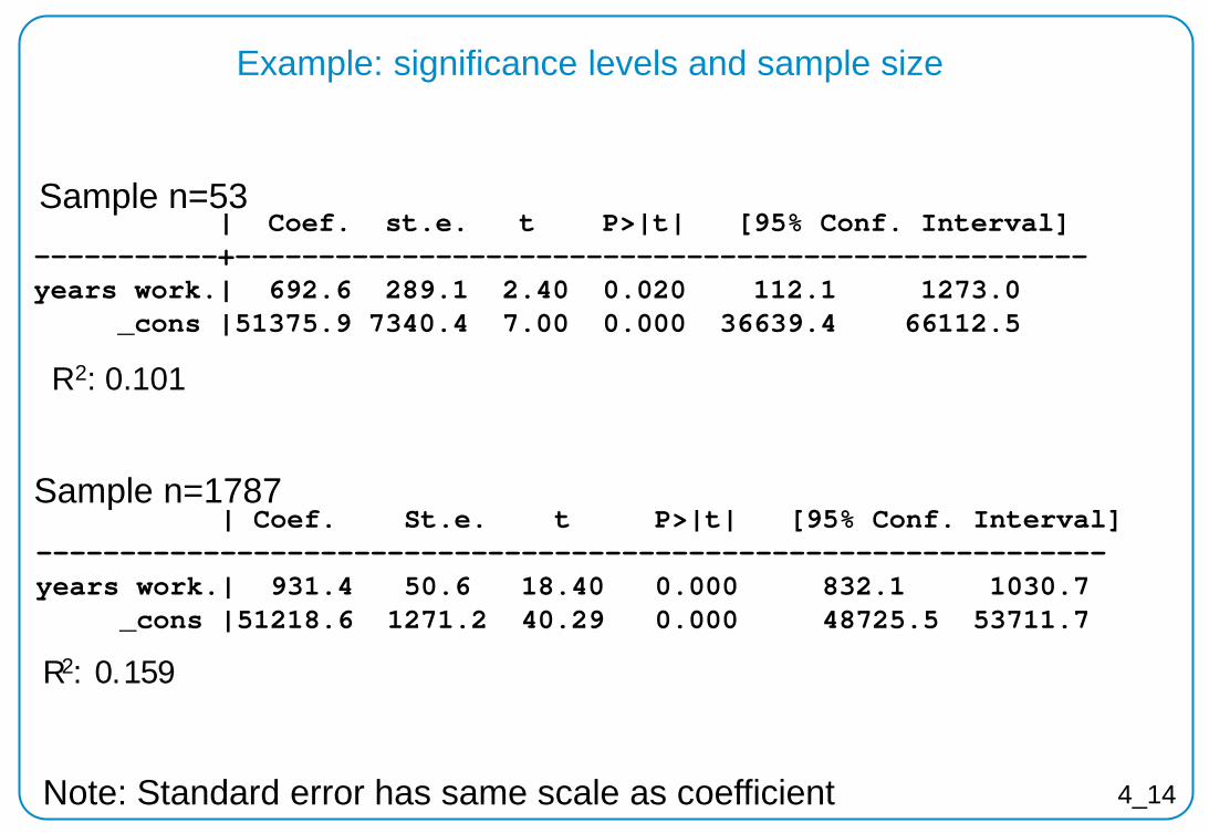
Example: significance levels and sample size
| Coef. st.e. t P>|t| [95% Conf. Interval] -----------+--------------------------------------------------- years work.| 692.6 289.1 2.40 0.020 112.1 1273.0 _cons |51375.9 7340.4 7.00 0.000 36639.4 66112.5
R2: 0.101
| Coef. St.e. t P>|t| [95% Conf. Interval] ---------------------------------------------------------------- years work.| 931.4 50.6 18.40 0.000 832.1 1030.7 _cons |51218.6 1271.2 40.29 0.000 48725.5 53711.7
R2: 0.159
Sample n=53
Sample n=1787
Note: Standard error has same scale as coefficient

4_15
Assumptions of OLS regression
General Continuous dependent variable Random sample
Coefficient estimation
No perfect multicollinearity E(e) = 0 (artifact) No endogeneity; Cov(x,e) = 0
Inference
• No autocorrelation Cov(ei,ek)=0 • Constant variance (no heteroscedasticity) • Preferentially: residuals normally distributed
Coefficients biased (inconsistent)
Standard errors of coefficients biased

4_16
Inference : assumptions
Assumptions on error terms – Independence of error terms , no autocorrelation:
Cov (εi, εk) = 0 for all i,k, i≠k – Constant error variance : Var(εi)=σ2
ε for all i; (Homoscedasticity)
Preferentially: e is normally distributed Matrix of error terms
2
2
2
2
2
2
2
00000000000010000000050000004000000300000020000001
154321;
σσ
σσ
σσ
σ
nn
nnki
−
−
4_17
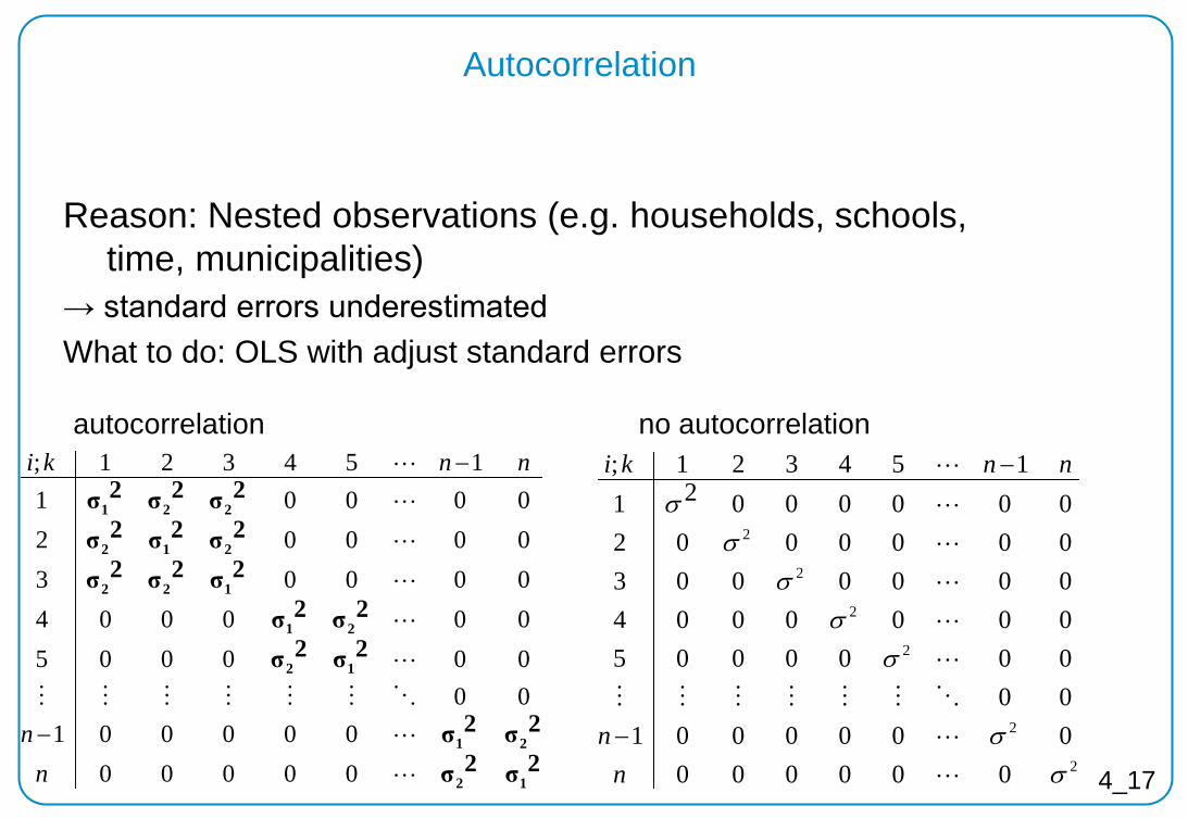
Autocorrelation
Reason: Nested observations (e.g. households, schools, time, municipalities)
→ standard errors underestimated What to do: OLS with adjust standard errors
2σ2σ
2σ2σ
2σ2σ
2σ2σ
2σ2σ2σ
2σ2σ2σ
2σ2σ2σ
12
21
12
21
122
212
221
00000000001
00000005000004000030000200001
154321;
nn
nnki
−
−
2
2
2
2
2
2
000000000000100000000500000040000003000000200000021
154321;
σσ
σσ
σσ
σ
nn
nnki
−
−autocorrelation no autocorrelation
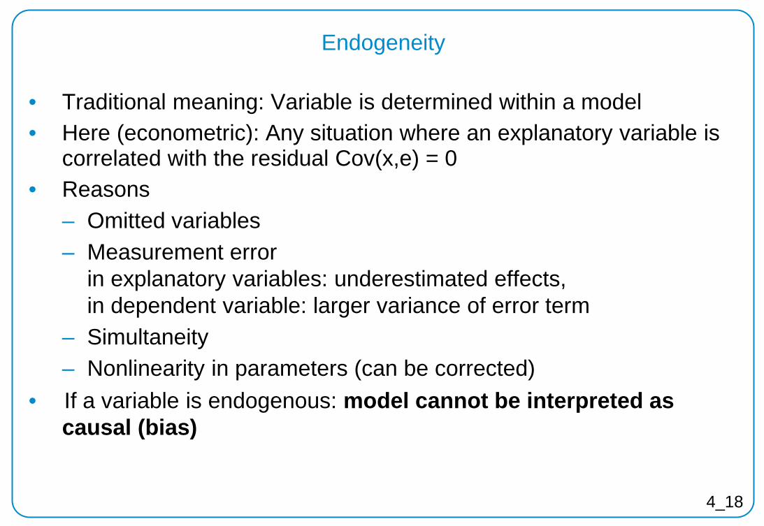
• Traditional meaning: Variable is determined within a model • Here (econometric): Any situation where an explanatory variable is
correlated with the residual Cov(x,e) = 0 • Reasons
– Omitted variables – Measurement error
in explanatory variables: underestimated effects, in dependent variable: larger variance of error term
– Simultaneity – Nonlinearity in parameters (can be corrected)
• If a variable is endogenous: model cannot be interpreted as causal (bias)
Endogeneity
4_18
4_19
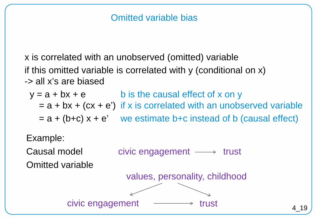
Omitted variable bias
x is correlated with an unobserved (omitted) variable if this omitted variable is correlated with y (conditional on x) -> all x’s are biased y = a + bx + e b is the causal effect of x on y = a + bx + (cx + e’) if x is correlated with an unobserved variable = a + (b+c) x + e’ we estimate b+c instead of b (causal effect) Example: Causal model civic engagement trust Omitted variable
values, personality, childhood
civic engagement trust
4_20
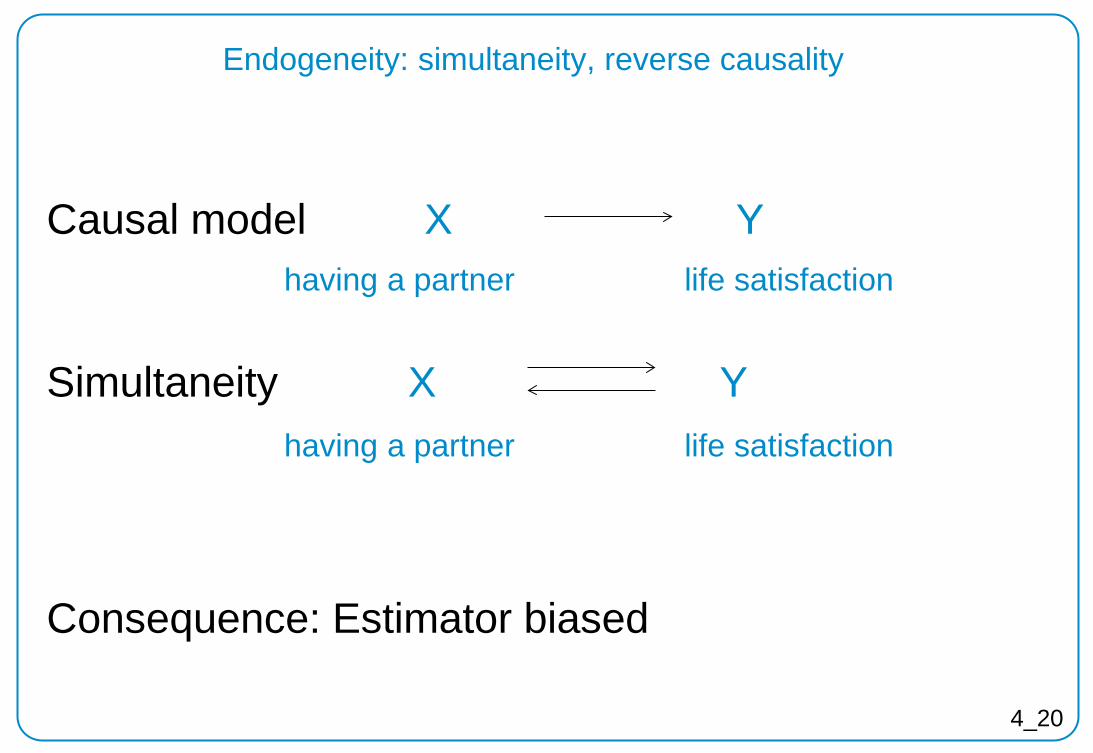
Endogeneity: simultaneity, reverse causality
Causal model X Y
Simultaneity X Y
Consequence: Estimator biased
having a partner
life satisfaction
life satisfaction
having a partner

Detection and correction of endogeneity
• Difficult: caution for causal interpretation! • Detection
‒ Theory, literature (variable selection and interpretation) !!!! ‒ Robustness checks
• Correction: instrumental variables, panel data (time ordering, within-models), structural equation modelling, discontinuity design….
• ! Overcontrol is common in social research based on regressions. Do not control for intervening mechanisms (“collider” variables)
4_21
4_22
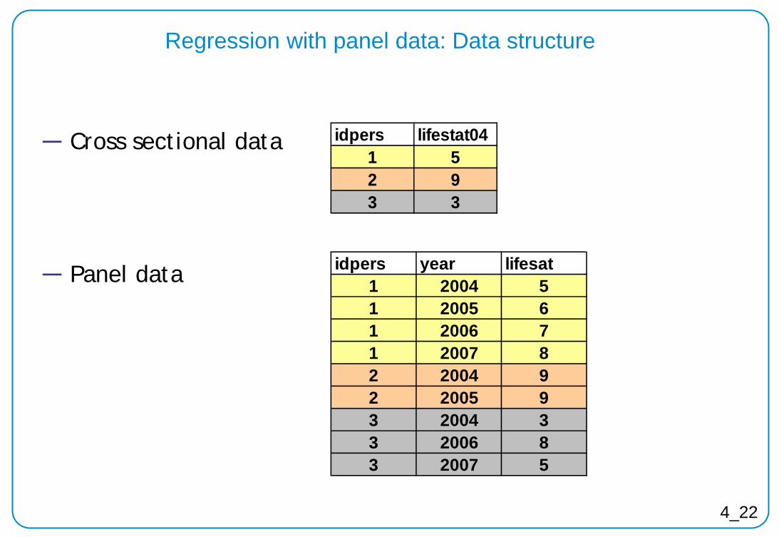
Regression with panel data: Data structure
― Cross sectional data ― Panel data
idpers year lifesat1 2004 51 2005 61 2006 71 2007 82 2004 92 2005 93 2004 33 2006 83 2007 5
idpers lifestat041 52 93 3
OLS with pooled panel data: problems I
• Pooled data: long data format, different years in one file • Problem: OLS assumption of independent observations
violated (autocorrelation) → coefficients unbiased → but standard errors biased (underestimation) • Possible measure: Correct for clustering in error terms • But: OLS is not the best estimator for pooled data (not
efficient)
4_23
4_24
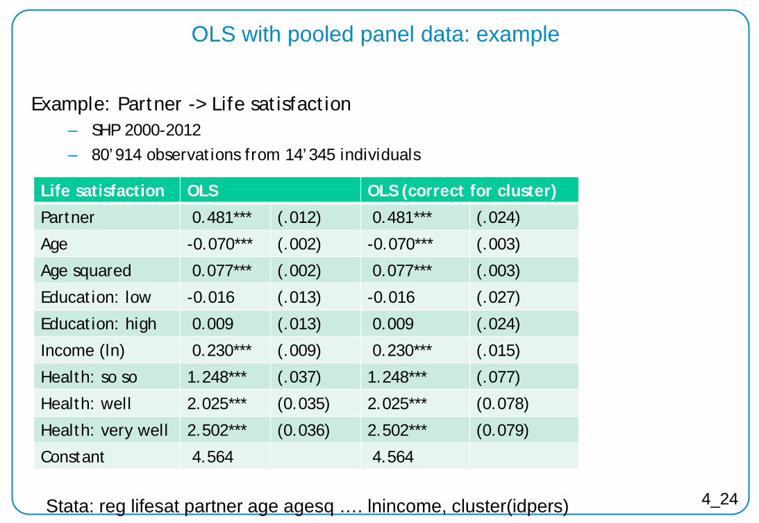
OLS with pooled panel data: example
Example: Partner -> Life satisfaction ‒ SHP 2000-2012 ‒ 80’914 observations from 14’345 individuals
Life satisfaction OLS OLS (correct for cluster)
Partner 0.481*** (.012) 0.481*** (.024)
Age -0.070*** (.002) -0.070*** (.003)
Age squared 0.077*** (.002) 0.077*** (.003)
Education: low -0.016 (.013) -0.016 (.027)
Education: high 0.009 (.013) 0.009 (.024)
Income (ln) 0.230*** (.009) 0.230*** (.015)
Health: so so 1.248*** (.037) 1.248*** (.077)
Health: well 2.025*** (0.035) 2.025*** (0.078)
Health: very well 2.502*** (0.036) 2.502*** (0.079)
Constant 4.564 4.564
Stata: reg lifesat partner age agesq …. lnincome, cluster(idpers)
4_25
OLS with panel data: problems II and outlook
• OLS does not take advantage of panel structure • Two different types of variation in panel data
‒ Variation within individuals ‒ Variation between individuals
• Control for unobservable variables (stable personal characteristics)
‒ Within-models ‒ Random Effect Models
(multilevel /random intercept / hierarchical model/ frailty for event history, mixed model)
5_1
5 Causality
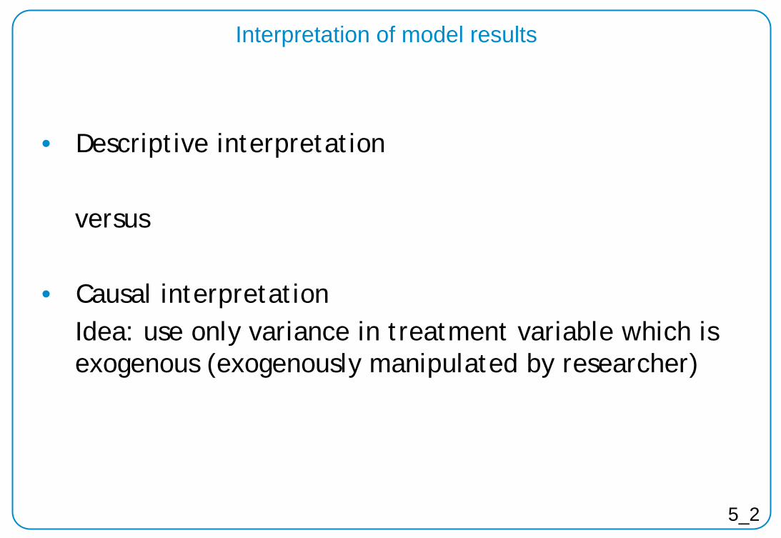
Interpretation of model results
• Descriptive interpretation versus • Causal interpretation Idea: use only variance in treatment variable which is exogenous (exogenously manipulated by researcher)
5_2
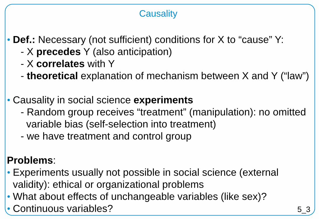
• Def.: Necessary (not sufficient) conditions for X to “cause” Y: - X precedes Y (also anticipation) - X correlates with Y - theoretical explanation of mechanism between X and Y (“law”)
• Causality in social science experiments - Random group receives “treatment” (manipulation): no omitted variable bias (self-selection into treatment) - we have treatment and control group Problems: • Experiments usually not possible in social science (external
validity): ethical or organizational problems • What about effects of unchangeable variables (like sex)? • Continuous variables?
Causality
5_3
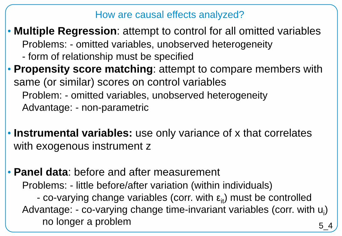
• Multiple Regression: attempt to control for all omitted variables Problems: - omitted variables, unobserved heterogeneity - form of relationship must be specified • Propensity score matching: attempt to compare members with
same (or similar) scores on control variables Problem: - omitted variables, unobserved heterogeneity Advantage: - non-parametric
• Instrumental variables: use only variance of x that correlates
with exogenous instrument z
• Panel data: before and after measurement Problems: - little before/after variation (within individuals) - co-varying change variables (corr. with εit) must be controlled Advantage: - co-varying change time-invariant variables (corr. with ui) no longer a problem
How are causal effects analyzed?
5_4
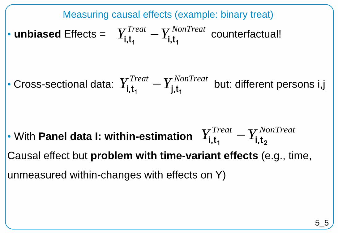
• unbiased Effects = counterfactual!
• Cross-sectional data: but: different persons i,j
• With Panel data I: within-estimation
Causal effect but problem with time-variant effects (e.g., time,
unmeasured within-changes with effects on Y)
NonTreatTreat YY11 tj,ti, −
NonTreatTreat YY11 ti,ti, −
Measuring causal effects (example: binary treat)
NonTreatTreat YY21 ti,ti, −
5_5

Between-estimation • ok with experimental data – Due to randomization units differ only in the treatment
• But strong assumption of unit homogeneity causes bias – Problem: self-selection into treatment! – Unobserved unit heterogeneity
Within-estimation • with control group often ok because the parallel trends
assumption is much weaker – Unobserved unit heterogeneity will not bias within-estimation
– Only differing time-trends in treatment and control group will bias within-estimation results
Basic Approach
5_6
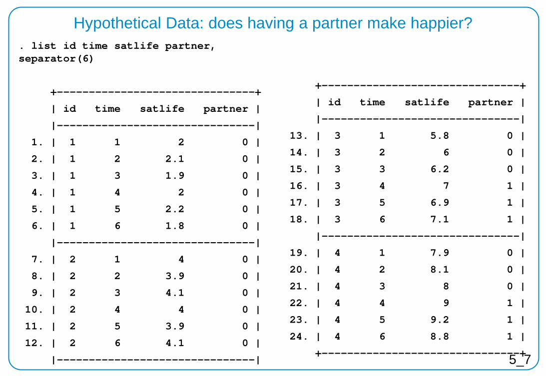
. list id time satlife partner, separator(6)
+-------------------------------+
| id time satlife partner |
|-------------------------------|
1. | 1 1 2 0 |
2. | 1 2 2.1 0 |
3. | 1 3 1.9 0 |
4. | 1 4 2 0 |
5. | 1 5 2.2 0 |
6. | 1 6 1.8 0 |
|-------------------------------|
7. | 2 1 4 0 |
8. | 2 2 3.9 0 |
9. | 2 3 4.1 0 |
10. | 2 4 4 0 |
11. | 2 5 3.9 0 |
12. | 2 6 4.1 0 |
|-------------------------------|
Hypothetical Data: does having a partner make happier?
5_7
+-------------------------------+
| id time satlife partner |
|-------------------------------|
13. | 3 1 5.8 0 |
14. | 3 2 6 0 |
15. | 3 3 6.2 0 |
16. | 3 4 7 1 |
17. | 3 5 6.9 1 |
18. | 3 6 7.1 1 |
|-------------------------------|
19. | 4 1 7.9 0 |
20. | 4 2 8.1 0 |
21. | 4 3 8 0 |
22. | 4 4 9 1 |
23. | 4 5 9.2 1 |
24. | 4 6 8.8 1 |
+-------------------------------+
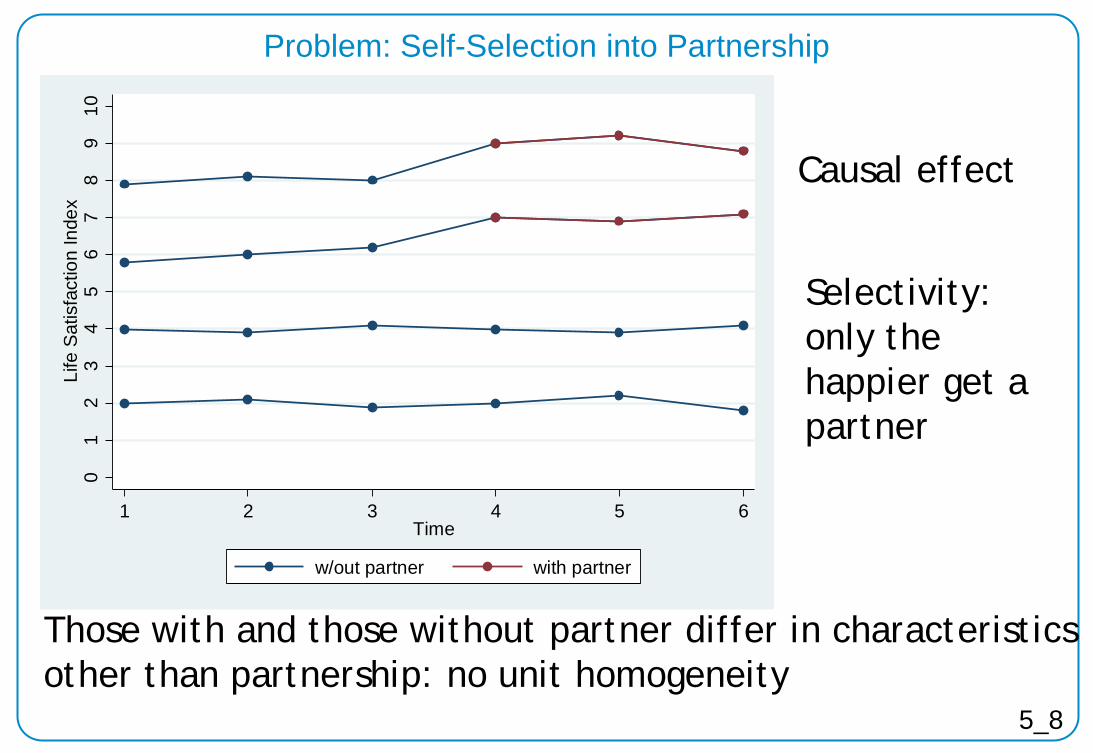
Problem: Self-Selection into Partnership
5_8
Those with and those without partner differ in characteristics other than partnership: no unit homogeneity
Causal effect
Selectivity: only the happier get a partner
01
23
45
67
89
10Li
fe S
atis
fact
ion
Inde
x
1 2 3 4 5 6Time
w/out partner with partner
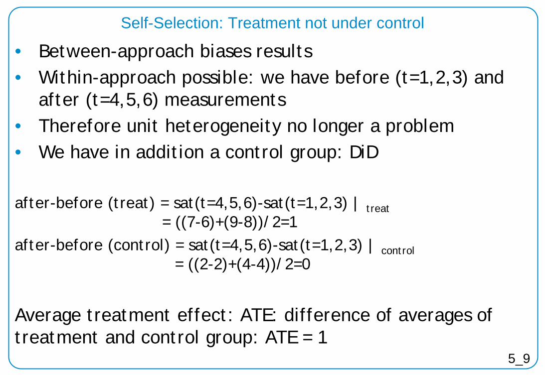
Self-Selection: Treatment not under control
5_9
• Between-approach biases results • Within-approach possible: we have before (t=1,2,3) and
after (t=4,5,6) measurements • Therefore unit heterogeneity no longer a problem • We have in addition a control group: DiD
after-before (treat) = sat(t=4,5,6)-sat(t=1,2,3) | treat
= ((7-6)+(9-8))/2=1 after-before (control) = sat(t=4,5,6)-sat(t=1,2,3) | control
= ((2-2)+(4-4))/2=0
Average treatment effect: ATE: difference of averages of treatment and control group: ATE = 1
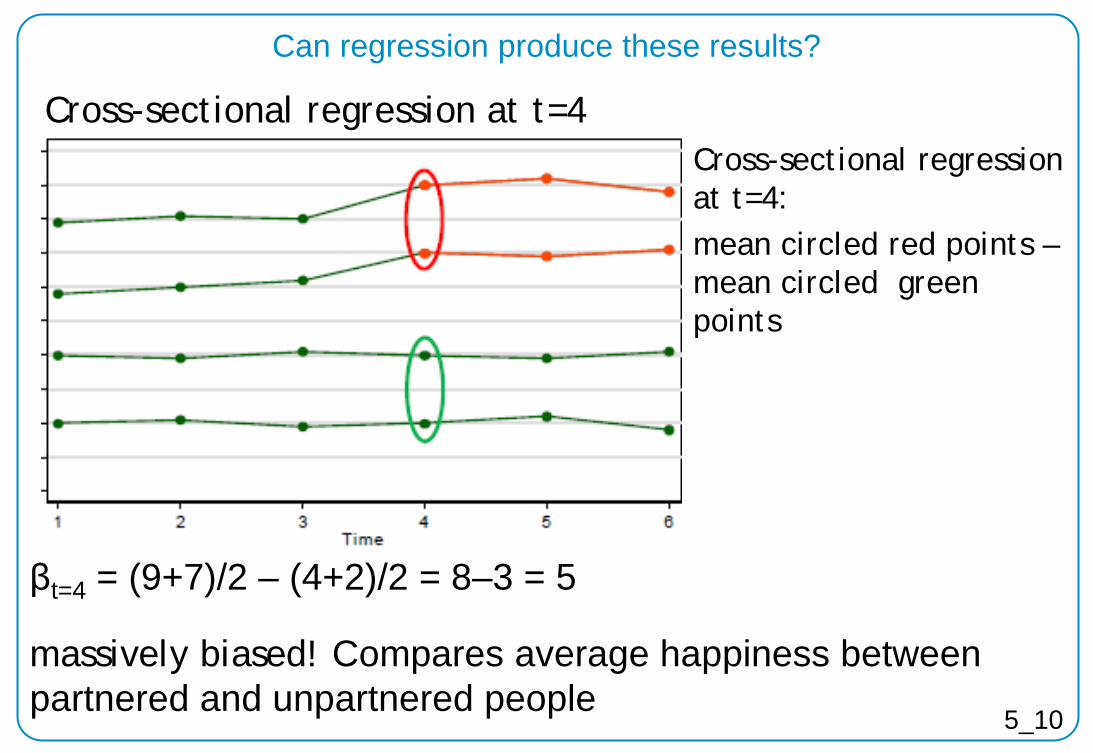
Can regression produce these results?
5_10
Cross-sectional regression at t=4
βt=4 = (9+7)/2 – (4+2)/2 = 8–3 = 5
massively biased! Compares average happiness between partnered and unpartnered people
Cross-sectional regression at t=4: mean circled red points – mean circled green points
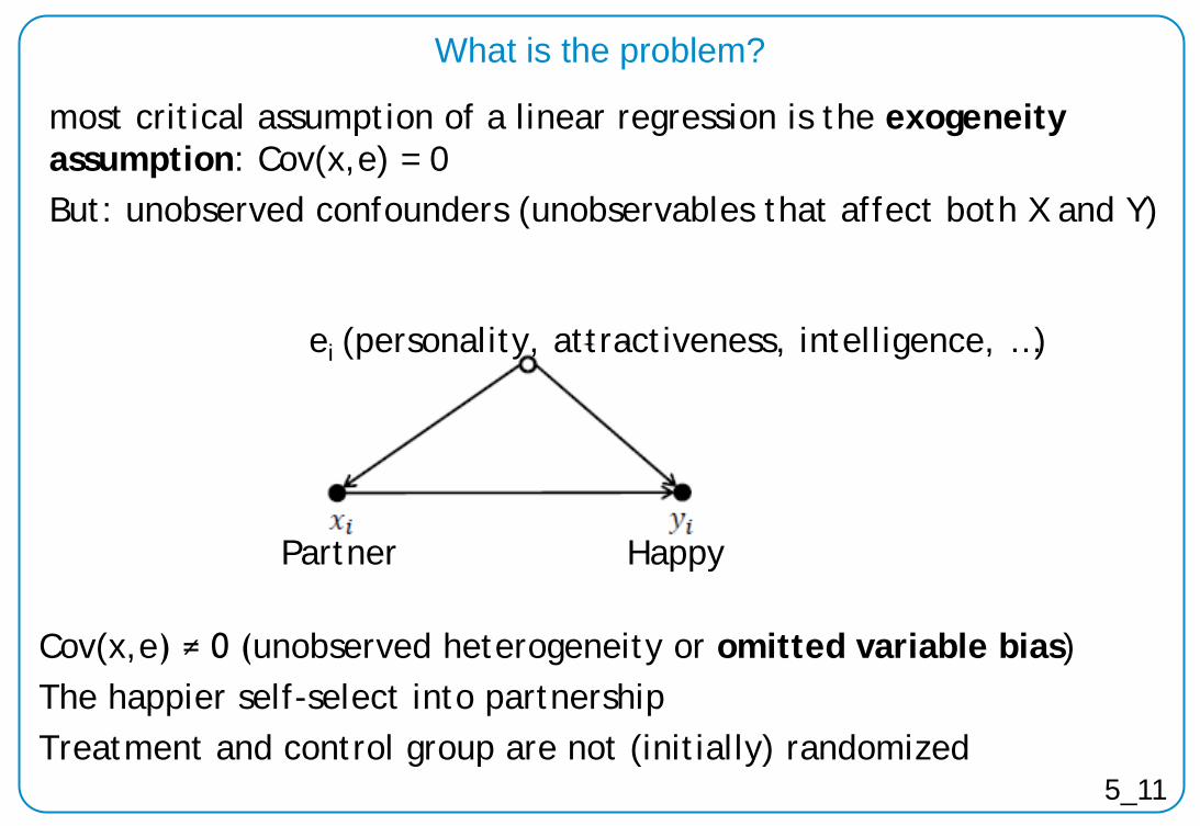
What is the problem?
5_11
most critical assumption of a linear regression is the exogeneity assumption: Cov(x,e) = 0 But: unobserved confounders (unobservables that affect both X and Y)
ei (personality, attractiveness, intelligence, …)
Partner Happy
Cov(x,e) ≠ 0 (unobserved heterogeneity or omitted variable bias) The happier self-select into partnership Treatment and control group are not (initially) randomized
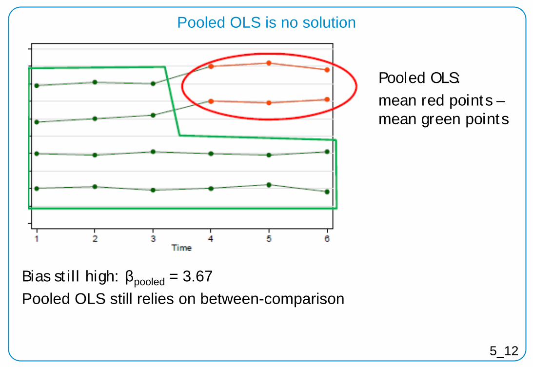
Pooled OLS is no solution
5_12
Bias still high: βpooled = 3.67 Pooled OLS still relies on between-comparison
Pooled OLS: mean red points – mean green points
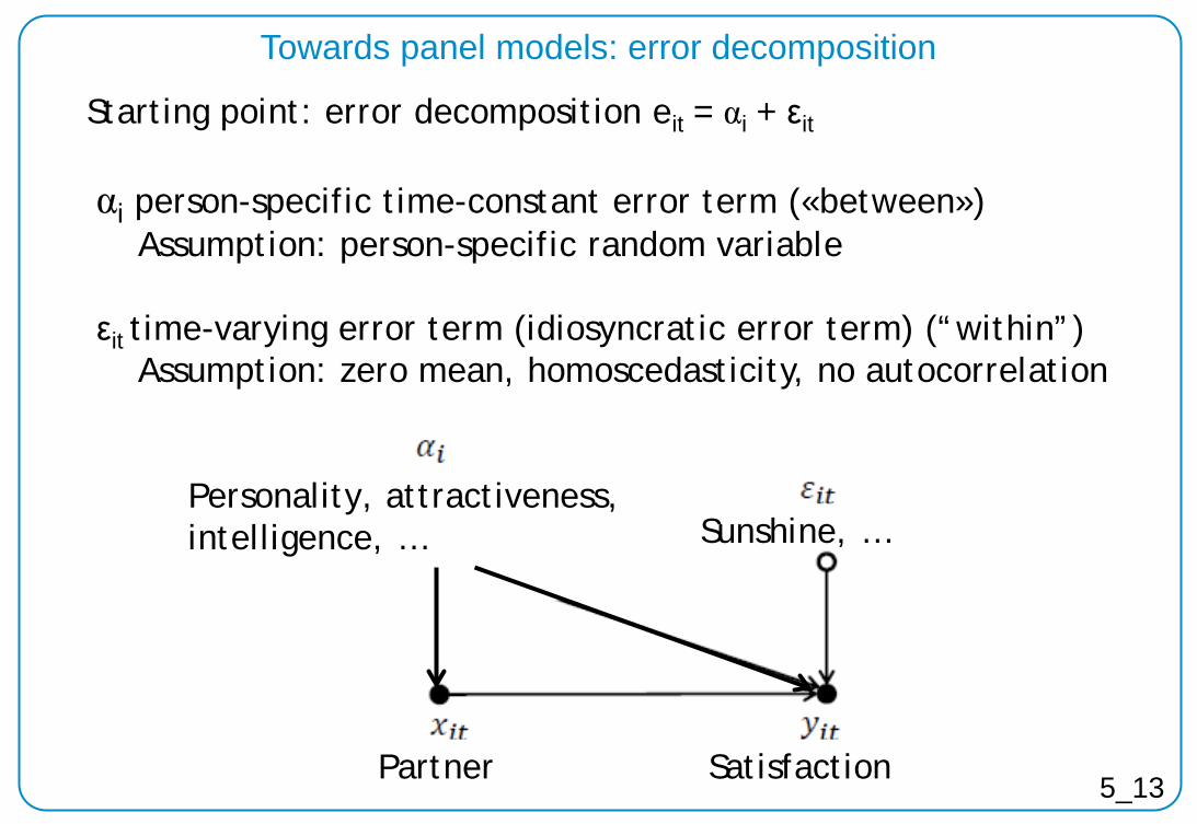
Starting point: error decomposition eit = αi + εit
αi person-specific time-constant error term («between») Assumption: person-specific random variable εit time-varying error term (idiosyncratic error term) (“within”) Assumption: zero mean, homoscedasticity, no autocorrelation
Towards panel models: error decomposition
Partner 5_13 Satisfaction Partner
Personality, attractiveness, intelligence, … Sunshine, …
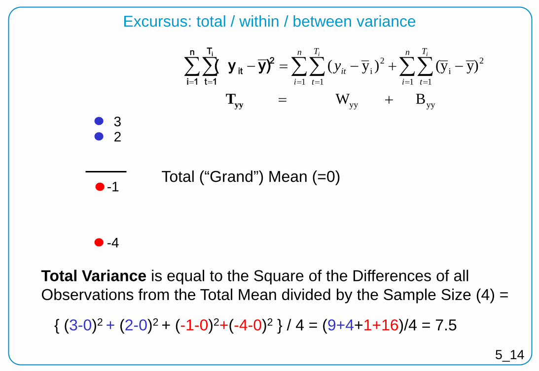
Total Variance is equal to the Square of the Differences of all Observations from the Total Mean divided by the Sample Size (4) =
{ (3-0)2 + (2-0)2 + (-1-0)2+(-4-0)2 } / 4 = (9+4+1+16)/4 = 7.5
Excursus: total / within / between variance
yyyy
1 1
2i
1 1
2i
B W
)yy()y(
+=
−+−=− ∑∑∑∑∑∑= == == =
yyT
n
i
T
t
n
i
T
tit
ii
yn
1i
T
1t
2it
i
)y( y
Total (“Grand”) Mean (=0)
3 2
-1
-4
5_14
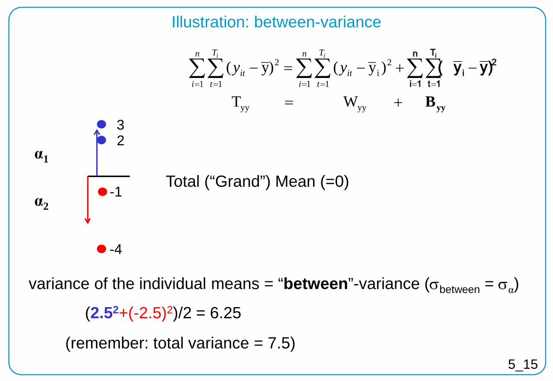
variance of the individual means = “between”-variance (σbetween = σα)
(remember: total variance = 7.5)
(2.52+(-2.5)2)/2 = 6.25
Illustration: between-variance
yyB W T
)y()y(
yyyy
1 1
2i
1 1
2
+=
−+−=− ∑∑∑∑∑∑= == == =
n
1i
T
1t
2i
i
)yy(n
i
T
tit
n
i
T
tit
ii
yy
Total (“Grand”) Mean (=0)
3 2
-1
-4
α1
α2
5_15
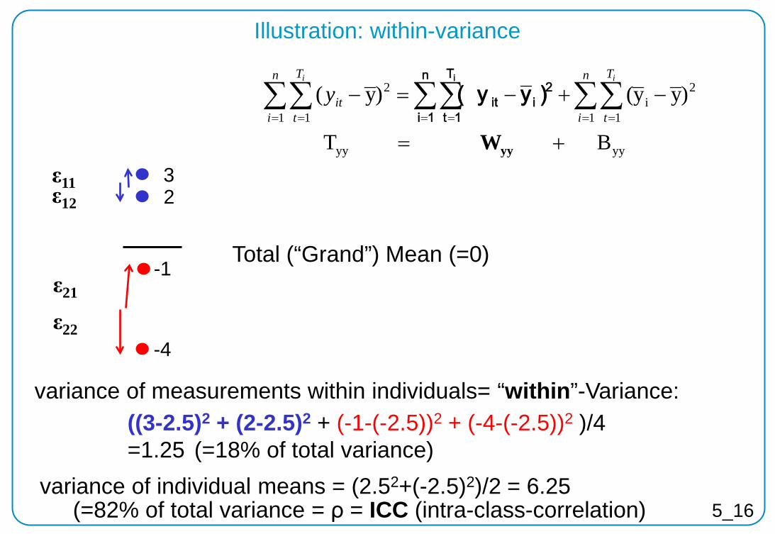
variance of measurements within individuals= “within”-Variance:
variance of individual means = (2.52+(-2.5)2)/2 = 6.25 (=82% of total variance = ρ = ICC (intra-class-correlation)
((3-2.5)2 + (2-2.5)2 + (-1-(-2.5))2 + (-4-(-2.5))2 )/4 =1.25 (=18% of total variance)
yyyy
1 1
2i
1 1
2
B T
)yy()y(
+=
−+−=− ∑∑∑∑∑∑= == == =
yyW
n
i
T
t
n
i
T
tit
ii
yn
1i
T
1t
2iit
i
)y( y
Total (“Grand”) Mean (=0)
3 2
-1
-4
Illustration: within-variance
ε11 ε12
ε21
ε22
5_16
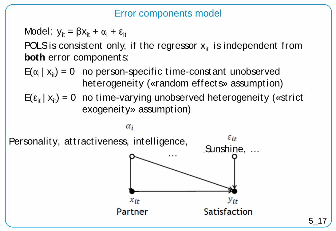
Model: yit = βxit + αi + εit
POLS is consistent only, if the regressor xit is independent from both error components: E(αi | xit) = 0 no person-specific time-constant unobserved heterogeneity («random effects» assumption) E(εit | xit) = 0 no time-varying unobserved heterogeneity («strict exogeneity» assumption)
Error components model
5_17
Personality, attractiveness, intelligence, … Sunshine, …
6 Fixed Effects (“within”)
Models
6-2
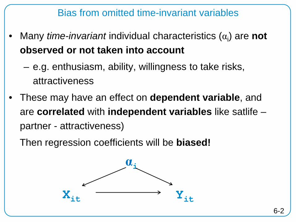
Bias from omitted time-invariant variables
• Many time-invariant individual characteristics (αi) are not observed or not taken into account – e.g. enthusiasm, ability, willingness to take risks,
attractiveness
• These may have an effect on dependent variable, and are correlated with independent variables like satlife – partner - attractiveness)
Then regression coefficients will be biased!
αi
Xit
Yit

Hypothetical Example:
Omitted time-invariant Variable Bias BMI (Y) and Smoking (X) : Continuous “Treatment”
6-3

21
2223
2425
2627
2829
3031
32bm
i
0 10 20 30 40cigarettes
BMI und Anzahl Zigaretten pro Tag
Hypothetical Observations: BMI and number of cigarettes per day
6-4
bmi
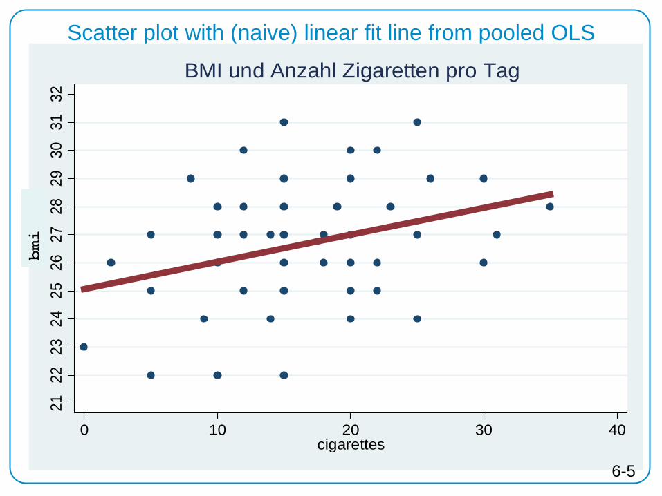
Scatter plot with (naive) linear fit line from pooled OLS 21
2223
2425
2627
2829
3031
32
0 10 20 30 40cigarettes
BMI und Anzahl Zigaretten pro Tag
6-5
bmi
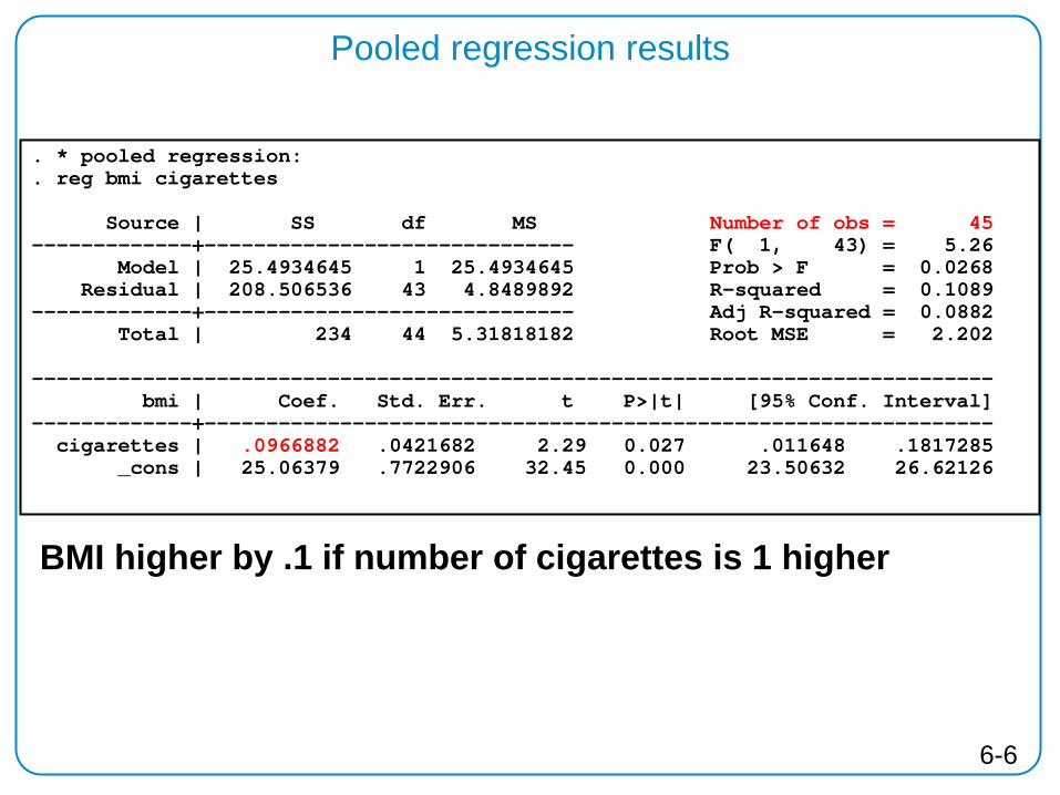
Pooled regression results
. * pooled regression:
. reg bmi cigarettes Source | SS df MS Number of obs = 45 -------------+------------------------------ F( 1, 43) = 5.26 Model | 25.4934645 1 25.4934645 Prob > F = 0.0268 Residual | 208.506536 43 4.8489892 R-squared = 0.1089 -------------+------------------------------ Adj R-squared = 0.0882 Total | 234 44 5.31818182 Root MSE = 2.202 ------------------------------------------------------------------------------ bmi | Coef. Std. Err. t P>|t| [95% Conf. Interval] -------------+---------------------------------------------------------------- cigarettes | .0966882 .0421682 2.29 0.027 .011648 .1817285 _cons | 25.06379 .7722906 32.45 0.000 23.50632 26.62126
BMI higher by .1 if number of cigarettes is 1 higher
6-6
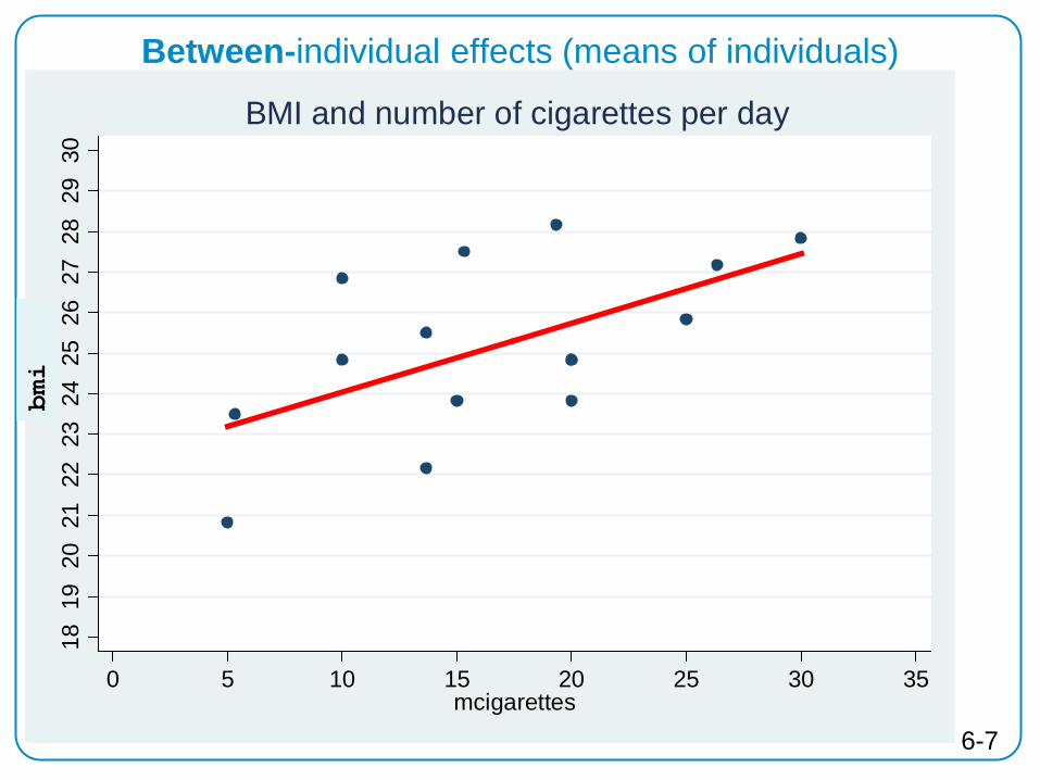
Between-individual effects (means of individuals) 21
2223
2425
2627
2829
3031
32
0 5 10 15 20 25 30 35 40mcigarettes
BMI and number of cigarettes per day18
1920
2122
2324
2526
2728
2930
0 5 10 15 20 25 30 35mcigarettes
BMI and number of cigarettes per day
6-7
bmi

Between regression
. * between-regression:
. egen mbmi=mean(bmi), by(id)
. egen mcigarettes=mean(cigarettes), by(id)
. bysort id: gen n=_n
. reg mbmi mcigarettes if n==1 // between-regression Source | SS df MS Number of obs = 15 -------------+------------------------------ F( 1, 13) = 6.98 Model | 22.134779 1 22.134779 Prob > F = 0.0203 Residual | 41.198548 13 3.16911908 R-squared = 0.3495 -------------+------------------------------ Adj R-squared = 0.2995 Total | 63.333327 14 4.52380907 Root MSE = 1.7802 ------------------------------------------------------------------------------ mbmi | Coef. Std. Err. t P>|t| [95% Conf. Interval] -------------+---------------------------------------------------------------- mcigarettes | .1709983 .0647029 2.64 0.020 .0312163 .3107803 _cons | 23.8319 1.166966 20.42 0.000 21.31082 26.35297 ------------------------------------------------------------------------------
BMI higher by .17 if number of cigarettes is 1 higher
6-8
2122
2324
2526
2728
2930
3132
0 10 20 30 40cigarettes
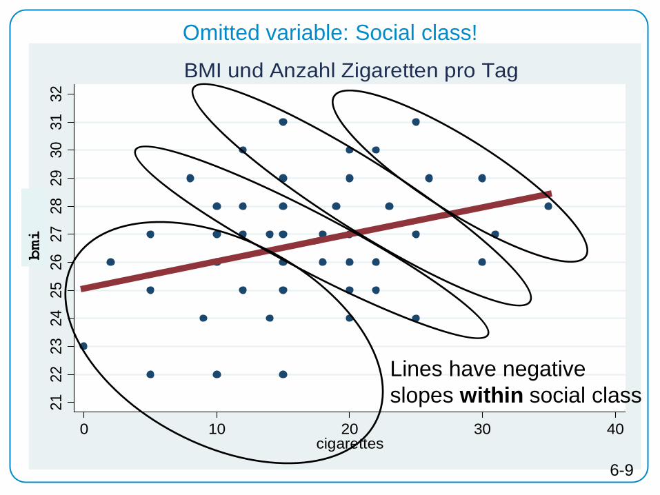
BMI und Anzahl Zigaretten pro Tag
Omitted variable: Social class!
Lines have negative slopes within social class
6-9
bmi
Panel Data is even better:
We can take a look within individuals
6-10

Panel Data: Observations are clustered in Individuals!
2122
2324
2526
2728
2930
3132
bmi
0 10 20 30 40cigarettes
BMI und Anzahl Zigaretten pro Tag
Lines have negative slopes within individuals
6-11
2122
2324
2526
2728
2930
3132
bmi
0 10 20 30 40cigarettes
BMI und Anzahl Zigaretten pro Tag22
2426
2830
32bm
i
0 10 20 30 40cigarettes
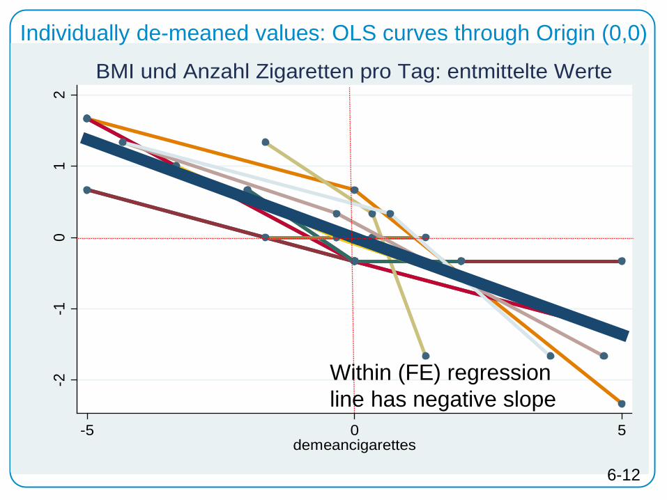
BMI und Anzahl Zigaretten pro Tag-2
-10
12
with
in
-5 0 5demeancigarettes
BMI und Anzahl Zigaretten pro Tag: entmittelte Werte-2
-10
12
-5 0 5demeancigarettes
BMI und Anzahl Zigaretten pro Tag: entmittelte Werte-2
-10
12
-5 0 5demeancigarettes
BMI und Anzahl Zigaretten pro Tag: entmittelte Werte
Individually de-meaned values: OLS curves through Origin (0,0)
Within (FE) regression line has negative slope
6-12

How can we calculate a within-regression
coefficient?
6-13
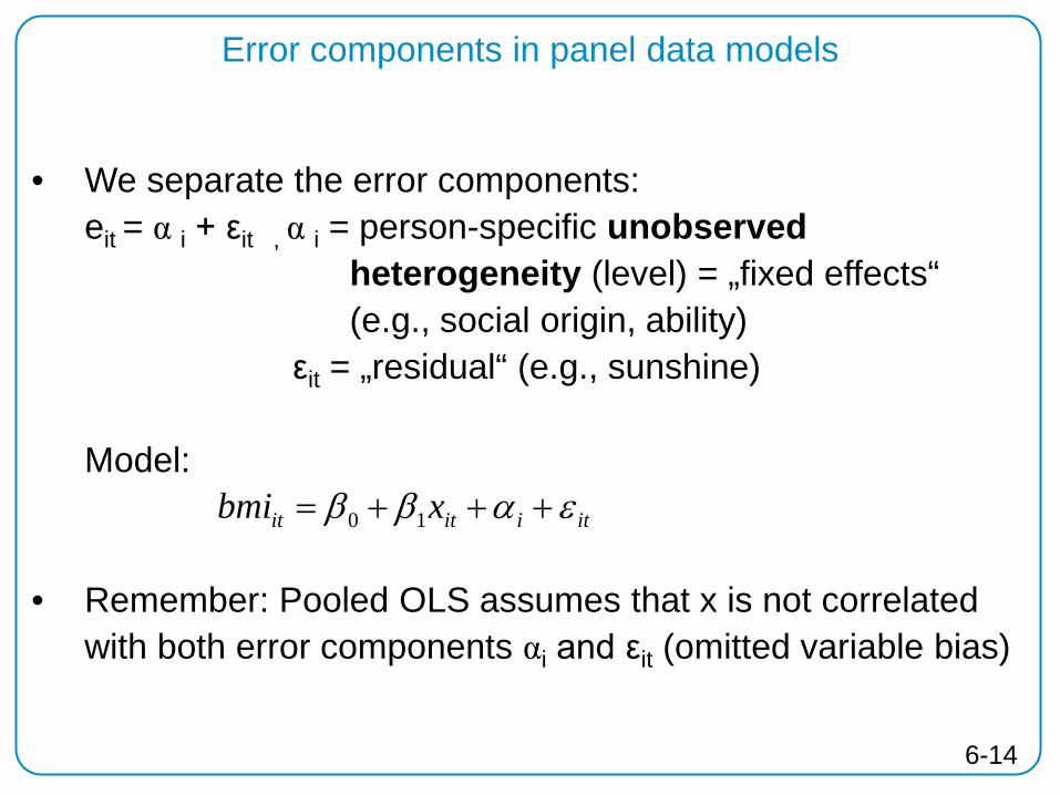
Error components in panel data models
• We separate the error components:
eit = α i + εit , α i = person-specific unobserved heterogeneity (level) = „fixed effects“ (e.g., social origin, ability)
εit = „residual“ (e.g., sunshine) Model:
• Remember: Pooled OLS assumes that x is not correlated with both error components αi and εit (omitted variable bias)
itiitit xbmi εαββ +++= 10
6-14
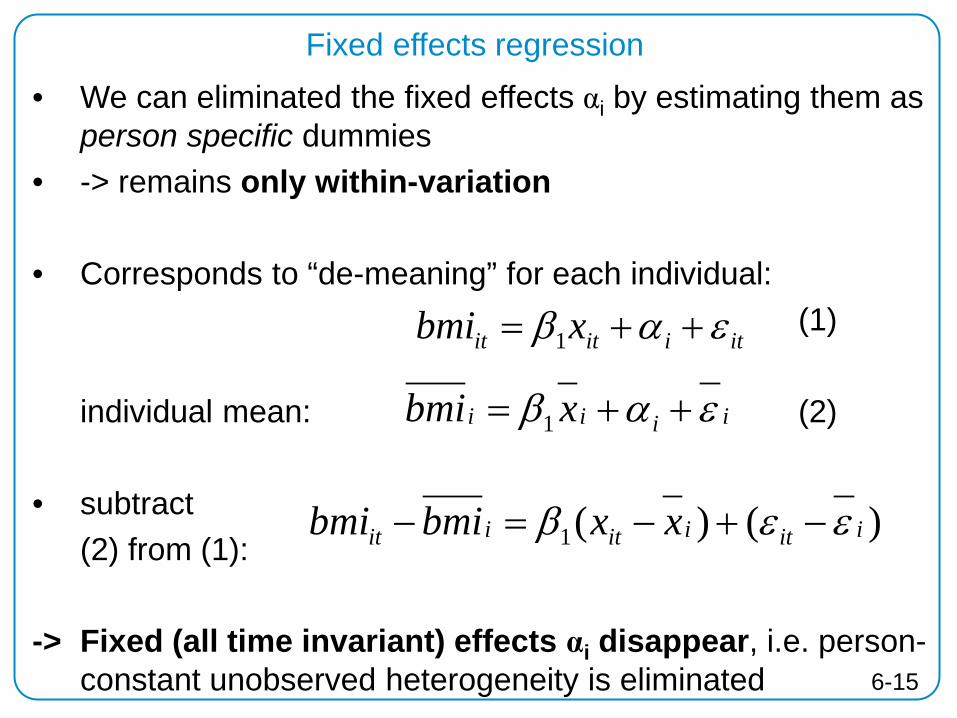
Fixed effects regression • We can eliminated the fixed effects αi by estimating them as
person specific dummies • -> remains only within-variation • Corresponds to “de-meaning” for each individual:
(1) individual mean: (2)
• subtract (2) from (1): -> Fixed (all time invariant) effects αi disappear, i.e. person-
constant unobserved heterogeneity is eliminated
itiitit xbmi εαβ ++= 1
iiii xbmi εαβ ++= 1
)()(1 iitiitiit xxbmibmi εεβ −+−=−
6-15
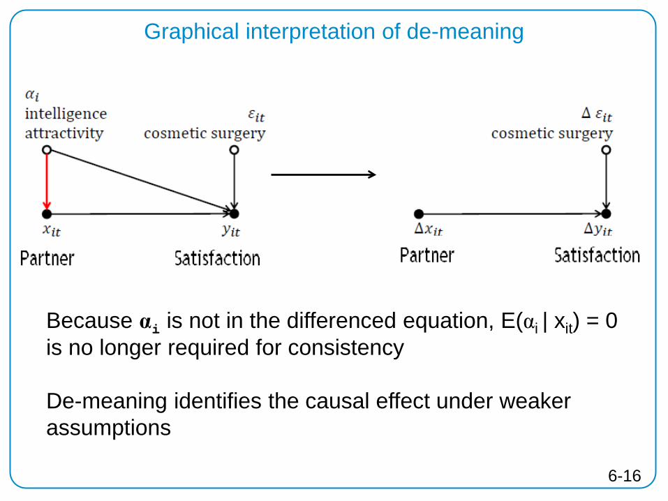
Graphical interpretation of de-meaning
6-16
Because αi is not in the differenced equation, E(αi | xit) = 0 is no longer required for consistency De-meaning identifies the causal effect under weaker assumptions
OLS of individually de-meaned Data
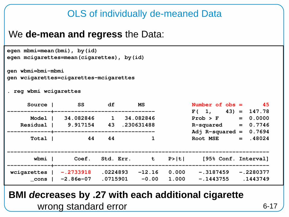
We de-mean and regress the Data: egen mbmi=mean(bmi), by(id) egen mcigarettes=mean(cigarettes), by(id) gen wbmi=bmi-mbmi gen wcigarettes=cigarettes-mcigarettes . reg wbmi wcigarettes Source | SS df MS Number of obs = 45 -------------+------------------------------ F( 1, 43) = 147.78 Model | 34.082846 1 34.082846 Prob > F = 0.0000 Residual | 9.917154 43 .230631488 R-squared = 0.7746 -------------+------------------------------ Adj R-squared = 0.7694 Total | 44 44 1 Root MSE = .48024 ------------------------------------------------------------------------------ wbmi | Coef. Std. Err. t P>|t| [95% Conf. Interval] -------------+---------------------------------------------------------------- wcigarettes | -.2733918 .0224893 -12.16 0.000 -.3187459 -.2280377 _cons | -2.86e-07 .0715901 -0.00 1.000 -.1443755 .1443749
BMI decreases by .27 with each additional cigarette wrong standard error 6-17

Direct modeling of fixed Effects in Stata
xtreg bmi time, fe (calculates correct df; this causes higher Std. Err.) . xtreg bmi cigarettes, fe Fixed-effects (within) regression Number of obs = 45 Group variable: id Number of groups = 15 R-sq: within = 0.7746 Obs per group: min = 3 between = 0.3495 avg = 3.0 overall = 0.1089 max = 3 F(1,29) = 99.67 corr(u_i, Xb) = -0.8080 Prob > F = 0.0000 ------------------------------------------------------------------------------ bmi | Coef. Std. Err. t P>|t| [95% Conf. Interval] -------------+---------------------------------------------------------------- cigarettes | -.2733918 .027385 -9.98 0.000 -.3294003 -.2173833 _cons | 31.1989 .4622757 67.49 0.000 30.25344 32.14436 -------------+---------------------------------------------------------------- sigma_u | 3.6906387 sigma_e | .58478272 rho | .97550841 (fraction of variance due to u_i) ------------------------------------------------------------------------------ F test that all u_i=0: F(14, 29) = 41.48 Prob > F = 0.0000 6-18
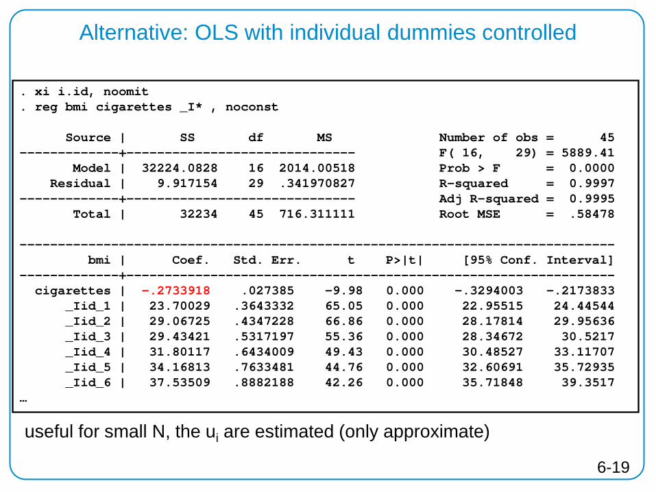
Alternative: OLS with individual dummies controlled
. xi i.id, noomit
. reg bmi cigarettes _I* , noconst Source | SS df MS Number of obs = 45 -------------+------------------------------ F( 16, 29) = 5889.41 Model | 32224.0828 16 2014.00518 Prob > F = 0.0000 Residual | 9.917154 29 .341970827 R-squared = 0.9997 -------------+------------------------------ Adj R-squared = 0.9995 Total | 32234 45 716.311111 Root MSE = .58478 ------------------------------------------------------------------------------ bmi | Coef. Std. Err. t P>|t| [95% Conf. Interval] -------------+---------------------------------------------------------------- cigarettes | -.2733918 .027385 -9.98 0.000 -.3294003 -.2173833 _Iid_1 | 23.70029 .3643332 65.05 0.000 22.95515 24.44544 _Iid_2 | 29.06725 .4347228 66.86 0.000 28.17814 29.95636 _Iid_3 | 29.43421 .5317197 55.36 0.000 28.34672 30.5217 _Iid_4 | 31.80117 .6434009 49.43 0.000 30.48527 33.11707 _Iid_5 | 34.16813 .7633481 44.76 0.000 32.60691 35.72935 _Iid_6 | 37.53509 .8882188 42.26 0.000 35.71848 39.3517 …
useful for small N, the ui are estimated (only approximate)
6-19
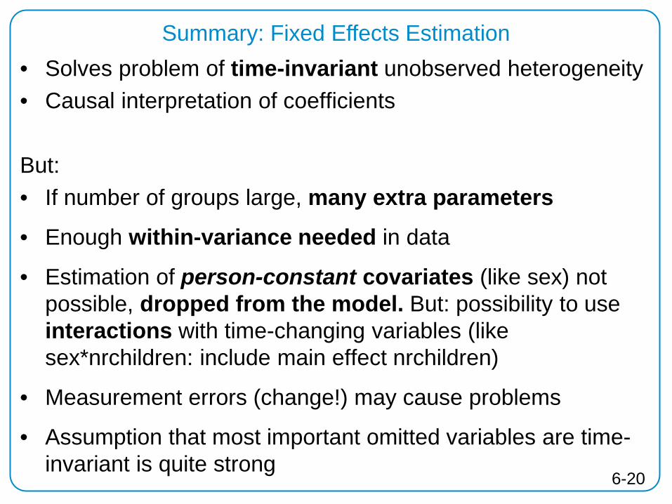
• Solves problem of time-invariant unobserved heterogeneity • Causal interpretation of coefficients But: • If number of groups large, many extra parameters
• Enough within-variance needed in data
• Estimation of person-constant covariates (like sex) not possible, dropped from the model. But: possibility to use interactions with time-changing variables (like sex*nrchildren: include main effect nrchildren)
• Measurement errors (change!) may cause problems
• Assumption that most important omitted variables are time-invariant is quite strong
Summary: Fixed Effects Estimation
6-20

Fixed Effects Model example from literature: Does civic engagement increase generalised trust?
Source: Van Ingen, E., & Bekkers, R. (2013). Generalized Trust Through Civic Engagement? Evidence from Five National Panel Studies. Political Psychology.
• Data: Swiss Household Panel 2004-2008 • Variables: − Y: Belief that most people can be trusted (scale 0 – 10) − X: Number of memberships in voluntary associations (0 - 9) − Control: Education, health, employment, having a partner
• Cross-sectional interpretation : compare trust of members/non-members with more or less membership
• Longitudinal interpretation : does trust change once individuals join or quit organisations? 6-21
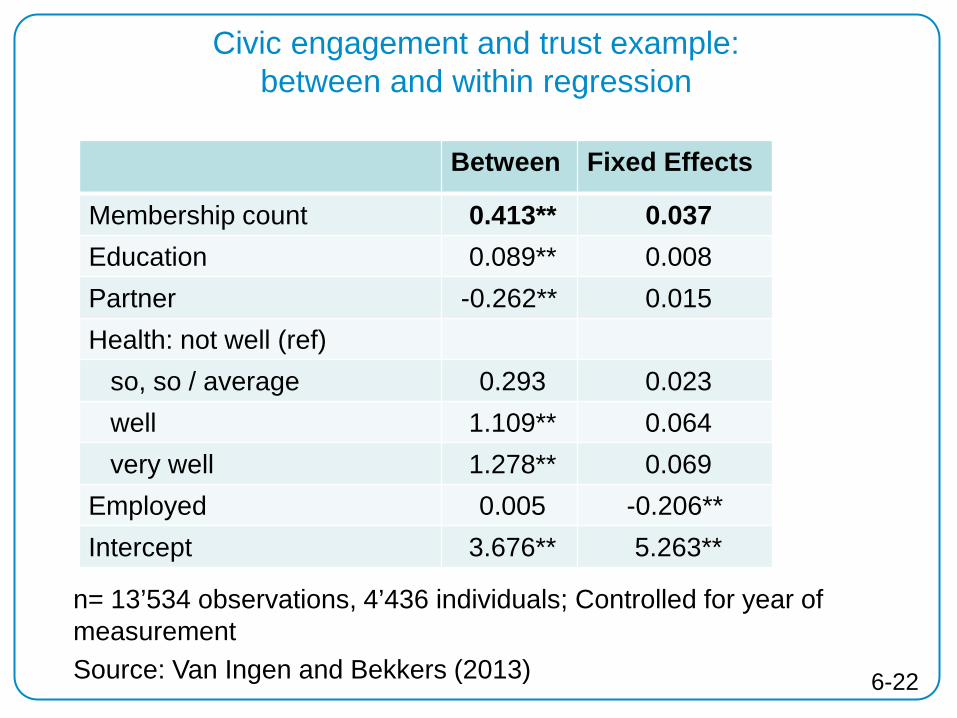
Civic engagement and trust example: between and within regression
Between Fixed Effects
Membership count 0.413** 0.037 Education 0.089** 0.008 Partner -0.262** 0.015 Health: not well (ref) so, so / average 0.293 0.023 well 1.109** 0.064 very well 1.278** 0.069 Employed 0.005 -0.206** Intercept 3.676** 5.263**
n= 13’534 observations, 4’436 individuals; Controlled for year of measurement Source: Van Ingen and Bekkers (2013) 6-22

Civic engagement and trust: assumptions / limitations of FE model
• All transitions are assumed to have the same effect (general assumption of linear regression)
– Effects of joining and quitting an organisation are
symmetric – Effect of maintaining 4 memberships (4-4) and staying
uninvolved (0-0) are equal
In addition: • Other life events may impact both membership and trust
(third variable)
6-23
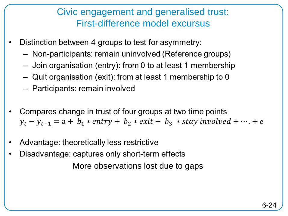
Civic engagement and generalised trust: First-difference model excursus
6-24
More observations lost due to gaps

Graphical interpretation of First-difference model
6-25
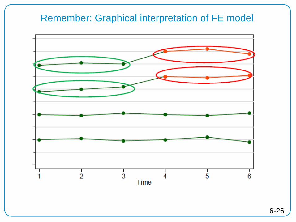
Remember: Graphical interpretation of FE model
6-26
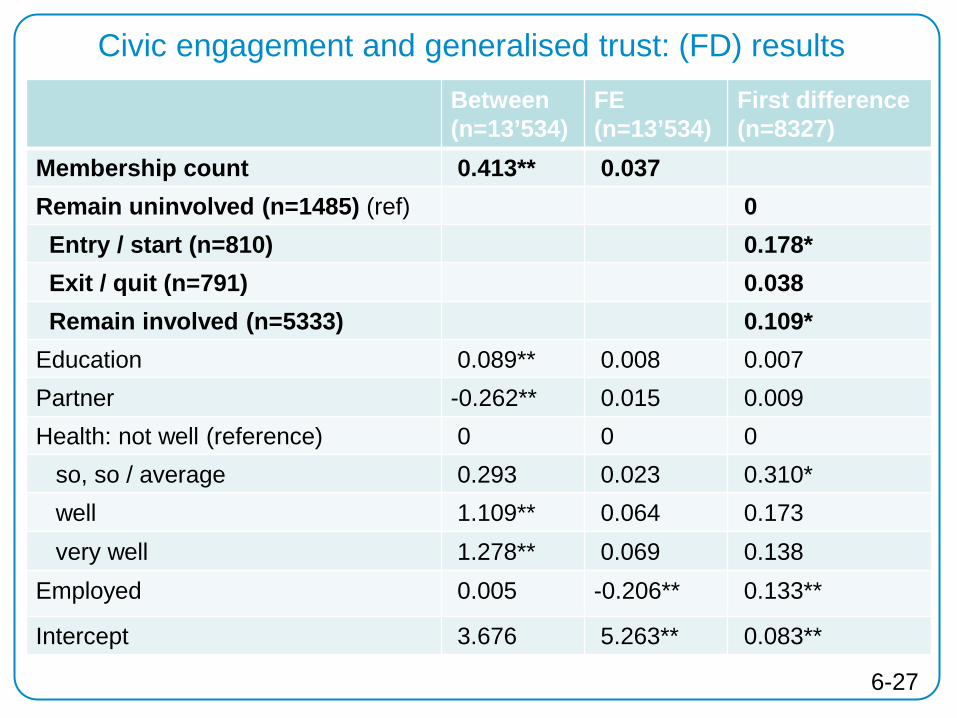
Civic engagement and generalised trust: (FD) results
Between (n=13’534)
FE (n=13’534)
First difference (n=8327)
Membership count 0.413** 0.037 Remain uninvolved (n=1485) (ref) 0 Entry / start (n=810) 0.178* Exit / quit (n=791) 0.038 Remain involved (n=5333) 0.109* Education 0.089** 0.008 0.007 Partner -0.262** 0.015 0.009 Health: not well (reference) 0 0 0 so, so / average 0.293 0.023 0.310* well 1.109** 0.064 0.173 very well 1.278** 0.069 0.138 Employed 0.005 -0.206** 0.133**
Intercept 3.676 5.263** 0.083**
6-27

Counterfactual of treated
Control group (j)
Treated (i)
t2 t1
In reality, treatment effect is positive!
What if we have a treatment which does not account for general developments (e.g., trend)?
With Panel data II: “difference-in-difference” (DID):
Assumption: parallel
trends
6-28
)()( NonTreatNonTreatTreatTreat YYYY1212 tj,tj,ti,ti, −−−
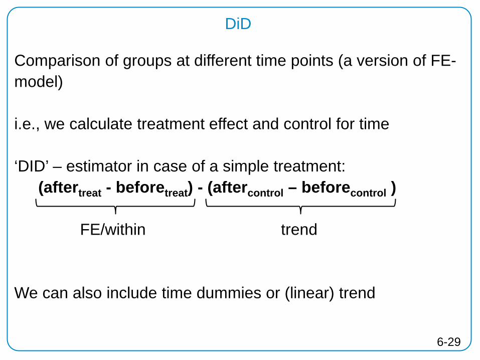
DiD
Comparison of groups at different time points (a version of FE-model)
i.e., we calculate treatment effect and control for time ‘DID’ – estimator in case of a simple treatment: (aftertreat - beforetreat) - (aftercontrol – beforecontrol ) FE/within trend We can also include time dummies or (linear) trend
6-29
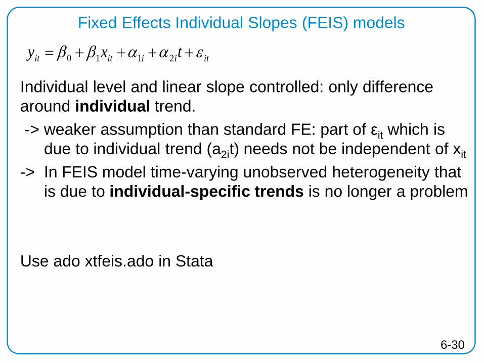
Fixed Effects Individual Slopes (FEIS) models
Individual level and linear slope controlled: only difference around individual trend. -> weaker assumption than standard FE: part of εit which is
due to individual trend (a2it) needs not be independent of xit
-> In FEIS model time-varying unobserved heterogeneity that is due to individual-specific trends is no longer a problem
Use ado xtfeis.ado in Stata
itiiitit txy εααββ ++++= 2110
6-30
7
Random Effects Models
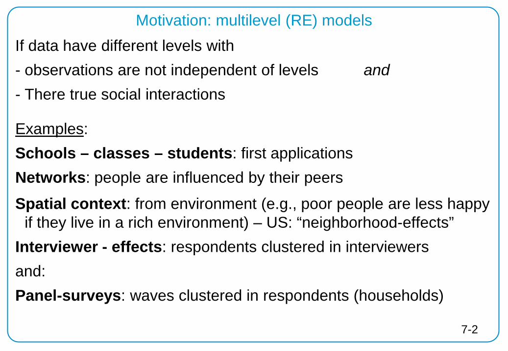
If data have different levels with - observations are not independent of levels and - There true social interactions
Examples: Schools – classes – students: first applications Networks: people are influenced by their peers
Spatial context: from environment (e.g., poor people are less happy if they live in a rich environment) – US: “neighborhood-effects”
Interviewer - effects: respondents clustered in interviewers and: Panel-surveys: waves clustered in respondents (households)
Motivation: multilevel (RE) models
7-2

Within versus cross-sectional research questions
“Within”– “causal” effects of time-variant variables: → modeling intrapersonal change (FE models) Cross-sectional – association with time-invariant effects: → OLS with robust standard errors In unbalanced panels: → RE models
Interpretation (e.g. presence of children): within: effect of additional children between: differences between people with a different number of
children
7-3

Starting point RE: “null” (“Variance Components” (VC)) model
:iondecomposit cefor varian allows model VC the
within"" assumed); )σ(N(0,mean specific individual fromdeviation εbetween"" assumed); )σ(N(0, variablerandom specific individual
:wheremodel) VCin aintercept no :(note
εit
u00i
0
==
+=
α
εα itiity
necessary) model multilevel tsignifican ρ :(note
Panels) in ationautocorrel ncorrelatio-class-intraICC( σσ
σρ
:i individual an withint points time different between ncorrelatio ρ
2ε
2u0
2u0
→
===+
=
=
7-4
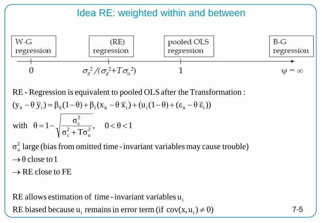
0))ucov(x, (if error termin remains u because biased RE u variablesinvariant - timeof estimation allows RE
FE toclose RE1 toclose θ
trouble)causemay variablesinvariant - timeomitted from (bias large σ
1θ0 ,Tσσ
σ1θwith
))ε θ(εθ)(1(u)x θ(xβθ)(1β)y θ(y:tionTransforma after the OLS pooled toequivalent is Regression -RE
ii
i
2u
2u
2ε
2ε
iitiiit10iit
≠
→→
<<+
−=
−+−+−+−=−
Idea RE: weighted within and between
7-5
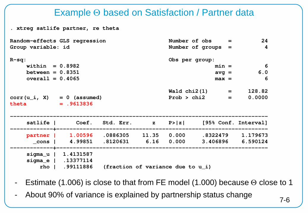
Example Θ based on Satisfaction / Partner data . xtreg satlife partner, re theta Random-effects GLS regression Number of obs = 24 Group variable: id Number of groups = 4 R-sq: Obs per group: within = 0.8982 min = 6 between = 0.8351 avg = 6.0 overall = 0.4065 max = 6 Wald chi2(1) = 128.82 corr(u_i, X) = 0 (assumed) Prob > chi2 = 0.0000 theta = .9613836 ------------------------------------------------------------------------------ satlife | Coef. Std. Err. z P>|z| [95% Conf. Interval] -------------+---------------------------------------------------------------- partner | 1.00596 .0886305 11.35 0.000 .8322479 1.179673 _cons | 4.99851 .8120631 6.16 0.000 3.406896 6.590124 -------------+---------------------------------------------------------------- sigma_u | 1.4131587 sigma_e | .13377114 rho | .99111886 (fraction of variance due to u_i)
7-6
- Estimate (1.006) is close to that from FE model (1.000) because Θ close to 1 - About 90% of variance is explained by partnership status change
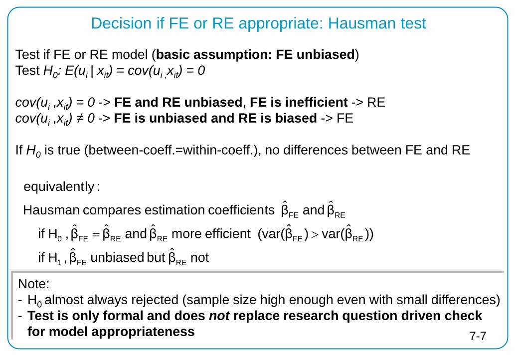
Decision if FE or RE appropriate: Hausman test
Test if FE or RE model (basic assumption: FE unbiased) Test H0: E(ui | xit) = cov(ui ,xit) = 0 cov(ui ,xit) = 0 -> FE and RE unbiased, FE is inefficient -> RE cov(ui ,xit) ≠ 0 -> FE is unbiased and RE is biased -> FE If H0 is true (between-coeff.=within-coeff.), no differences between FE and RE
not β but unbiased β , H if
))βvar( )β(var( efficient more β and β β , H if
β and β tscoefficien estimation compares Hausman
:lyequivalent
REFE1
REFEREREFE0
REFE
ˆˆ
ˆˆˆˆˆ
ˆˆ
>=
Note: - H0 almost always rejected (sample size high enough even with small differences) - Test is only formal and does not replace research question driven check
for model appropriateness 7-7
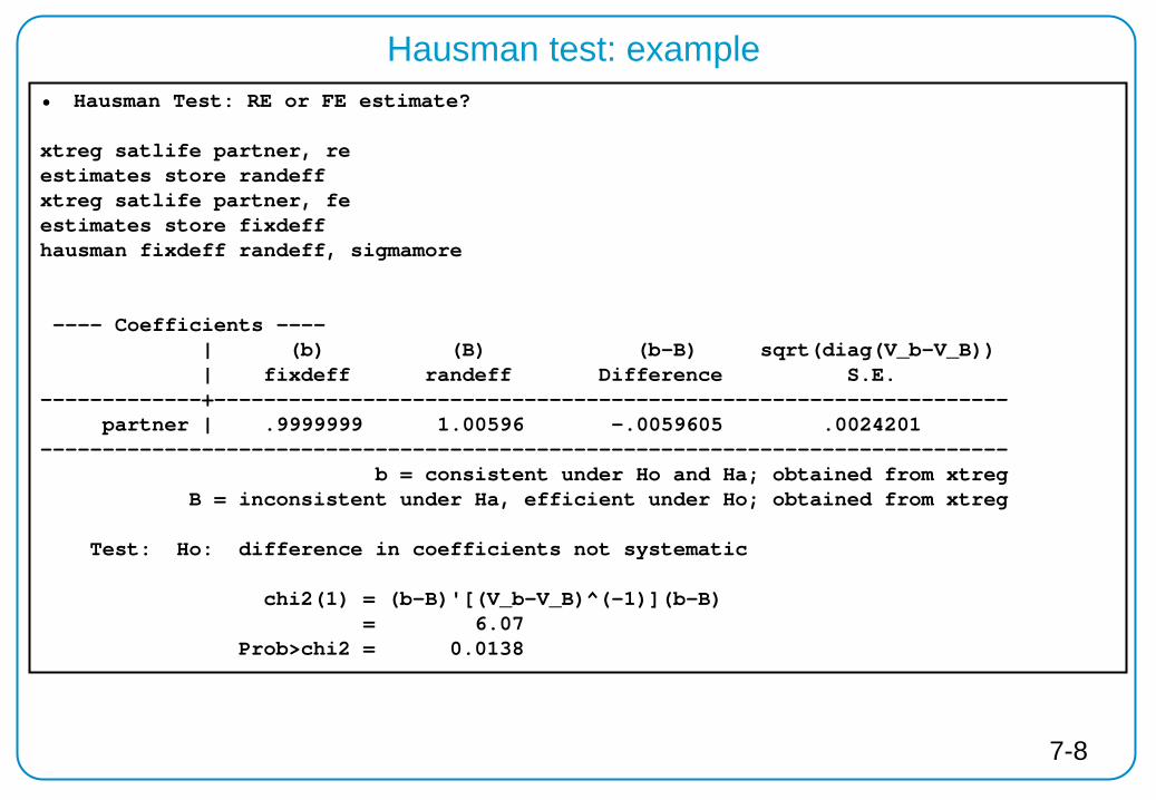
Hausman test: example • Hausman Test: RE or FE estimate?
xtreg satlife partner, re estimates store randeff xtreg satlife partner, fe estimates store fixdeff hausman fixdeff randeff, sigmamore ---- Coefficients ---- | (b) (B) (b-B) sqrt(diag(V_b-V_B)) | fixdeff randeff Difference S.E. -------------+---------------------------------------------------------------- partner | .9999999 1.00596 -.0059605 .0024201 ------------------------------------------------------------------------------ b = consistent under Ho and Ha; obtained from xtreg B = inconsistent under Ha, efficient under Ho; obtained from xtreg Test: Ho: difference in coefficients not systematic chi2(1) = (b-B)'[(V_b-V_B)^(-1)](b-B) = 6.07 Prob>chi2 = 0.0138
7-8
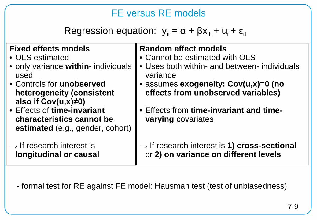
FE versus RE models
Fixed effects models • OLS estimated • only variance within- individuals
used • Controls for unobserved
heterogeneity (consistent also if Cov(u,x)≠0)
• Effects of time-invariant characteristics cannot be estimated (e.g., gender, cohort)
→ If research interest is longitudinal or causal
Random effect models • Cannot be estimated with OLS • Uses both within- and between- individuals
variance • assumes exogeneity: Cov(u,x)=0 (no
effects from unobserved variables)
• Effects from time-invariant and time-varying covariates
→ If research interest is 1) cross-sectional
or 2) on variance on different levels
Regression equation: yit = α + βxit + ui + εit
- formal test for RE against FE model: Hausman test (test of unbiasedness)
7-9
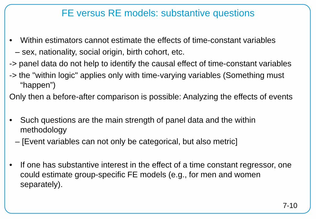
FE versus RE models: substantive questions
• Within estimators cannot estimate the effects of time-constant variables – sex, nationality, social origin, birth cohort, etc. -> panel data do not help to identify the causal effect of time-constant variables -> the "within logic" applies only with time-varying variables (Something must
“happen”) Only then a before-after comparison is possible: Analyzing the effects of events • Such questions are the main strength of panel data and the within
methodology – [Event variables can not only be categorical, but also metric] • If one has substantive interest in the effect of a time constant regressor, one
could estimate group-specific FE models (e.g., for men and women separately).
7-10
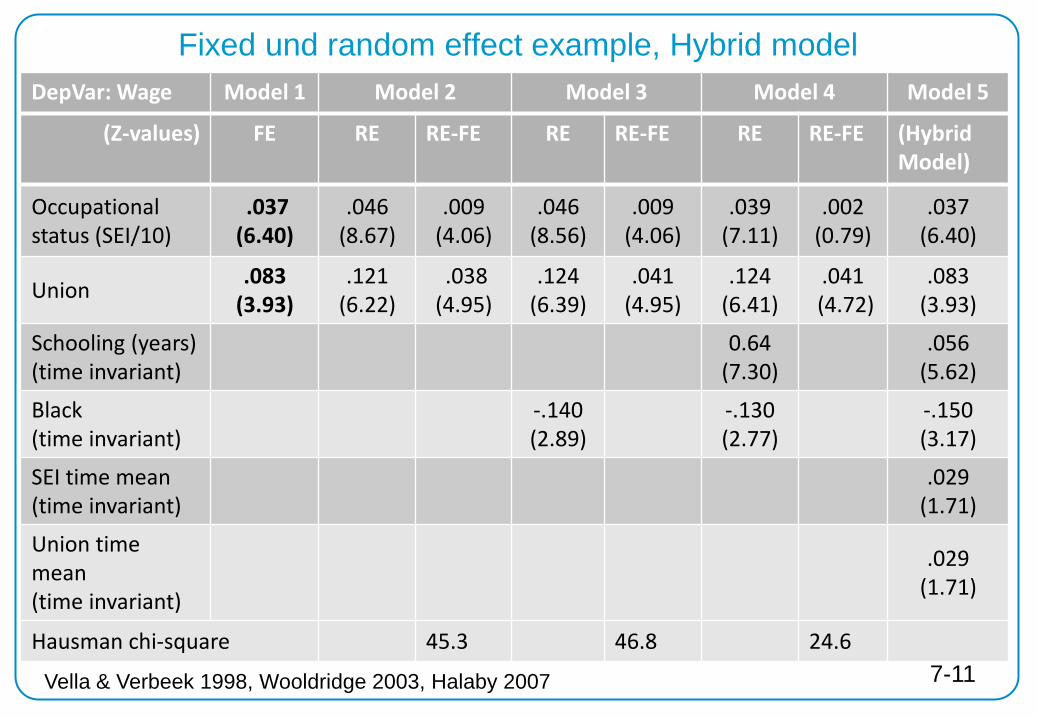
Fixed und random effect example, Hybrid model DepVar: Wage Model 1 Model 2 Model 3 Model 4 Model 5
(Z-values) FE RE RE-FE RE RE-FE RE RE-FE (Hybrid Model)
Occupational status (SEI/10)
.037 (6.40)
.046 (8.67)
.009 (4.06)
.046 (8.56)
.009 (4.06)
.039 (7.11)
.002 (0.79)
.037 (6.40)
Union .083 (3.93)
.121 (6.22)
.038 (4.95)
.124 (6.39)
.041 (4.95)
.124 (6.41)
.041 (4.72)
.083 (3.93)
Schooling (years) (time invariant)
0.64 (7.30)
.056 (5.62)
Black (time invariant)
-.140 (2.89)
-.130 (2.77)
-.150 (3.17)
SEI time mean (time invariant)
.029 (1.71)
Union time mean (time invariant)
.029 (1.71)
Hausman chi-square 45.3 46.8 24.6
Vella & Verbeek 1998, Wooldridge 2003, Halaby 2007 7-11

8
Non linear regression
Non-linear regression: motivation
Linear regression: requires continuous dependent variable e.g. BMI, income, satisfaction on scale from 0-10 (?)
Most variables in social science are not continuous but discrete – Opinions: agree vs. disagree – Poverty status – Party voted for – Number of visits to the doctor – Having a partner
We need appropriate regression models!
8-2

Non-linear models
Dependent variable is not continuous: non-linear regression
Binary variables (dummy variables, 0 or 1) (e.g. yes-no, event – no event)
Logistic Regression, Probit Regression, and many more
Multinomial (unordered variables) (e.g. vote choice, occupation)
Multinomal logistic Regression Multinomial probit Regression
Ordinal (e.g. satisfaction)
Ordinal Regression
Count variable (e.g. doctor visits)
Poisson Regression Negative Binomial Regression
7-3 8-3
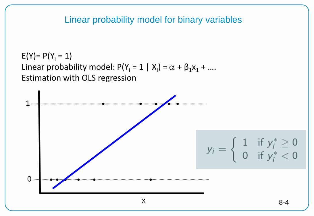
Linear probability model for binary variables
0
x
1
E(Y)= P(Yi = 1) Linear probability model: P(Yi = 1 | Xi) = α + β1x1 + …. Estimation with OLS regression
8-4
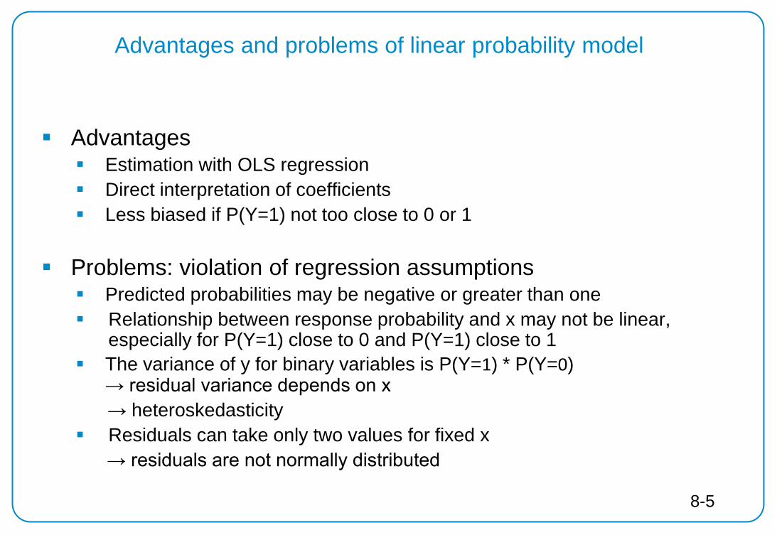
Advantages and problems of linear probability model
Advantages Estimation with OLS regression Direct interpretation of coefficients Less biased if P(Y=1) not too close to 0 or 1
Problems: violation of regression assumptions
Predicted probabilities may be negative or greater than one Relationship between response probability and x may not be linear,
especially for P(Y=1) close to 0 and P(Y=1) close to 1 The variance of y for binary variables is P(Y=1) * P(Y=0)
→ residual variance depends on x → heteroskedasticity Residuals can take only two values for fixed x → residuals are not normally distributed
8-5

P(Y=1) between 0 and 1 Non-linear Symmetry Often used function:
Cumulative logistic distribution (Logit model)
Other functions also used (e.g. probit). For practical purposes, these models provide very similar predicted probabilities
S-shaped function
...)( 221111)1Pr( +++−+
== xxey ββα
8-6
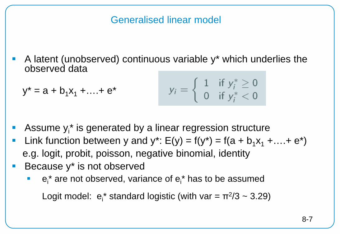
Generalised linear model
A latent (unobserved) continuous variable y* which underlies the observed data
y* = a + b1x1 +….+ e*
Assume yi* is generated by a linear regression structure Link function between y and y*: E(y) = f(y*) = f(a + b1x1 +….+ e*) e.g. logit, probit, poisson, negative binomial, identity Because y* is not observed ei* are not observed, variance of ei* has to be assumed
Logit model: ei* standard logistic (with var = π2/3 ~ 3.29)
7-7 8-7

Maximum likelihood estimation (MLE)
Usually, non-linear models are estimated by maximum likelihood Principle for MLE: Which set of parameters has the highest
likelihood to generate the data actually observed (xi, yi)? Advantages
Extremely flexible and can easily handle both linear and non-linear models (Linear model: MLE = OLS estimator)
Desirable asymptotic properties: consistency, efficiency, normality, (consistent if missing at random MAR)
Disadvantages Requires assumptions on distribution of residuals Desired properties hold only if model correctly specified Best suited for large samples
Often, there is no closed form (algebraic) solution. Coefficients have to be estimated through iteration methods
8-8
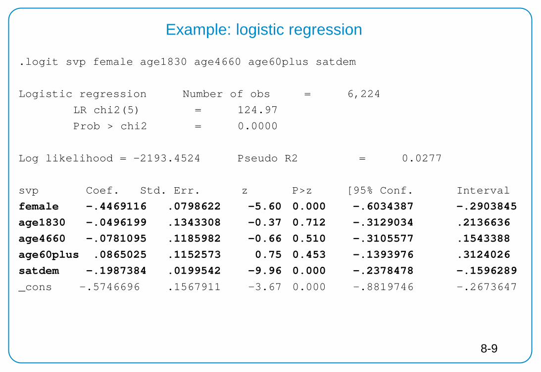
.logit svp female age1830 age4660 age60plus satdem
Logistic regression Number of obs = 6,224
LR chi2(5) = 124.97
Prob > chi2 = 0.0000
Log likelihood = -2193.4524 Pseudo R2 = 0.0277
svp Coef. Std. Err. z P>z [95% Conf. Interval
female -.4469116 .0798622 -5.60 0.000 -.6034387 -.2903845 age1830 -.0496199 .1343308 -0.37 0.712 -.3129034 .2136636 age4660 -.0781095 .1185982 -0.66 0.510 -.3105577 .1543388 age60plus .0865025 .1152573 0.75 0.453 -.1393976 .3124026 satdem -.1987384 .0199542 -9.96 0.000 -.2378478 -.1596289 _cons -.5746696 .1567911 -3.67 0.000 -.8819746 -.2673647
Example: logistic regression
8-9
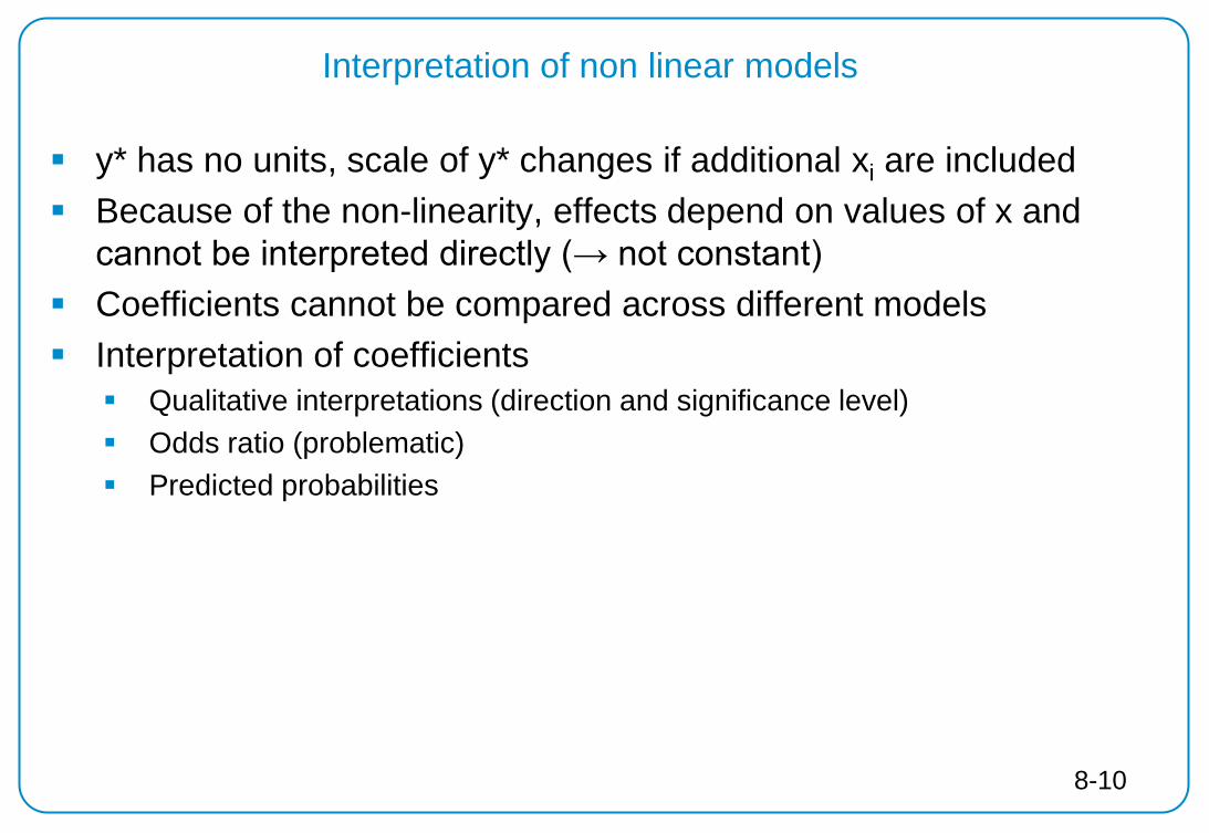
Interpretation of non linear models
y* has no units, scale of y* changes if additional xi are included Because of the non-linearity, effects depend on values of x and
cannot be interpreted directly (→ not constant) Coefficients cannot be compared across different models Interpretation of coefficients
Qualitative interpretations (direction and significance level) Odds ratio (problematic) Predicted probabilities
8-10

Excursus: Odds ratios (OR)
OR often misunderstood as relative risk
P A Group 1 0.10 0.11 2.10 2.00
Group 2 0.05 0.05 B Group 1 0.40 0.67 2.70 2.00
Group 2 0.20 0.25 C Group 1 0.80 4.00 6.00 2.00
Group 2 0.40 0.67 D Group 1 0.60 1.50 6.00 3.00
Group 2 0.20 0.25 E Group 1 0.40 0.67 6.00 4.00
Group 2 0.10 0.11
Ref.: Best and Wolf 2012, Kölner Zeitschrift für Soziologie 7-11 8-11
Compute predicted probabilities
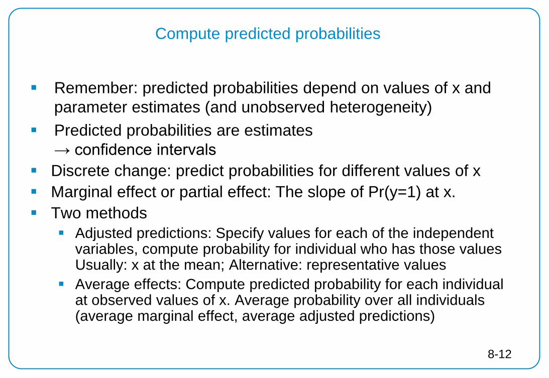
Remember: predicted probabilities depend on values of x and parameter estimates (and unobserved heterogeneity)
Predicted probabilities are estimates → confidence intervals
Discrete change: predict probabilities for different values of x Marginal effect or partial effect: The slope of Pr(y=1) at x. Two methods
Adjusted predictions: Specify values for each of the independent variables, compute probability for individual who has those values Usually: x at the mean; Alternative: representative values
Average effects: Compute predicted probability for each individual at observed values of x. Average probability over all individuals (average marginal effect, average adjusted predictions)
8-12
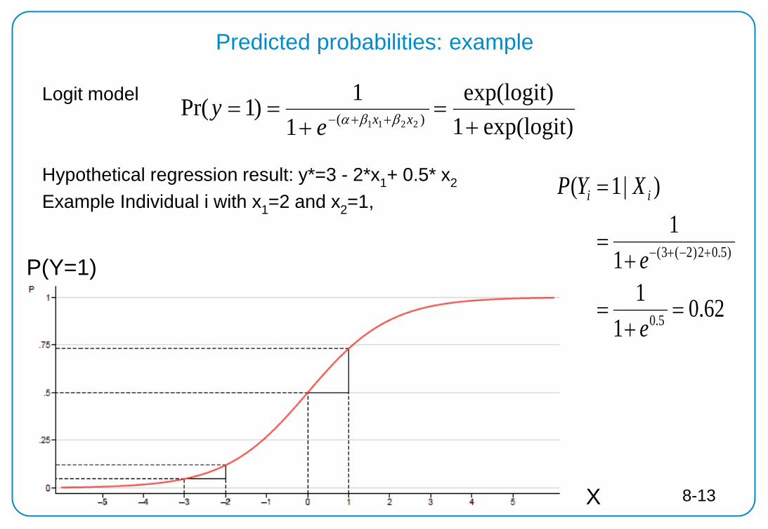
Predicted probabilities: example
Logit model Hypothetical regression result: y*=3 - 2*x1+ 0.5* x2
Example Individual i with x1=2 and x2=1,
exp(logit)1exp(logit)
11)1Pr( )( 2211 +
=+
== ++− xxey ββα
62.01
11
1)|1(
5.0
)5.02)2(3(
=+
=
+=
=
+−+−
e
e
XYP ii
P(Y=1)
X
Example: logistic regression
8-13
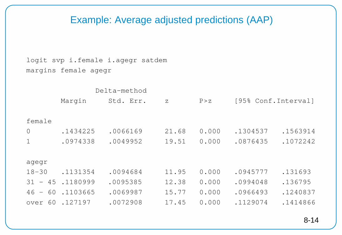
logit svp i.female i.agegr satdem
margins female agegr
Delta-method
Margin Std. Err. z P>z [95% Conf.Interval]
female
0 .1434225 .0066169 21.68 0.000 .1304537 .1563914
1 .0974338 .0049952 19.51 0.000 .0876435 .1072242
agegr
18-30 .1131354 .0094684 11.95 0.000 .0945777 .131693
31 - 45 .1180999 .0095385 12.38 0.000 .0994048 .136795
46 - 60 .1103665 .0069987 15.77 0.000 .0966493 .1240837
over 60 .127197 .0072908 17.45 0.000 .1129074 .1414866
Example: Average adjusted predictions (AAP)
8-14
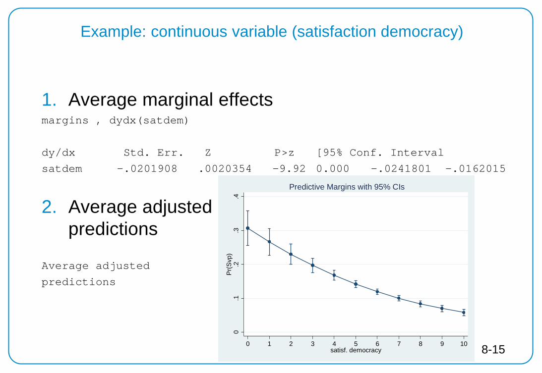
1. Average marginal effects margins , dydx(satdem)
dy/dx Std. Err. Z P>z [95% Conf. Interval
satdem -.0201908 .0020354 -9.92 0.000 -.0241801 -.0162015
2. Average adjusted predictions
Average adjusted
predictions
Example: continuous variable (satisfaction democracy)
0.1
.2.3
.4P
r(S
vp)
0 1 2 3 4 5 6 7 8 9 10satisf. democracy
Predictive Margins with 95% CIs
8-15
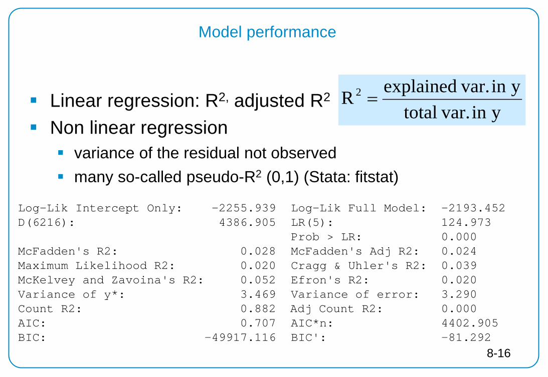
Model performance
Linear regression: R2, adjusted R2
Non linear regression variance of the residual not observed many so-called pseudo-R2 (0,1) (Stata: fitstat)
yin var.totalyin var.explainedR 2 =
Log-Lik Intercept Only: -2255.939 Log-Lik Full Model: -2193.452 D(6216): 4386.905 LR(5): 124.973 Prob > LR: 0.000 McFadden's R2: 0.028 McFadden's Adj R2: 0.024 Maximum Likelihood R2: 0.020 Cragg & Uhler's R2: 0.039 McKelvey and Zavoina's R2: 0.052 Efron's R2: 0.020 Variance of y*: 3.469 Variance of error: 3.290 Count R2: 0.882 Adj Count R2: 0.000 AIC: 0.707 AIC*n: 4402.905 BIC: -49917.116 BIC': -81.292
8-16
The likelihood ratio test
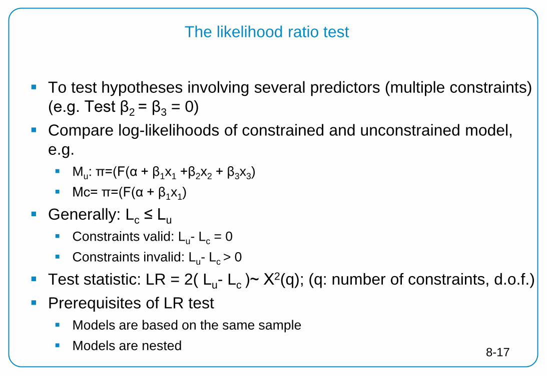
To test hypotheses involving several predictors (multiple constraints) (e.g. Test β2 = β3 = 0)
Compare log-likelihoods of constrained and unconstrained model, e.g. Mu: π=(F(α + β1x1 +β2x2 + β3x3) Mc= π=(F(α + β1x1)
Generally: Lc ≤ Lu Constraints valid: Lu- Lc = 0 Constraints invalid: Lu- Lc > 0
Test statistic: LR = 2( Lu- Lc )~ Х2(q); (q: number of constraints, d.o.f.) Prerequisites of LR test
Models are based on the same sample Models are nested 8-17

LR test example: test for joint significance
Vote intention model (support SVP vs. supporting another party P(Y = 1|X ) = F(α + β1(female) +β2(age)) +β3(lnincome) +β4(contra EU) +β5(for
nuclear energy) +β6(satisfaction democracy) Do demographic variables (age, sex) matter? H0: (β1,β2)=0
LR = 2( Lu- Lc )~=2*( -3762.1 – (-3772.2))=20.08 Chi-squared distribution with 2 degrees of freedom: p=0.0000
-> we reject H0 (demographic variables seem to affect the probability to vote for SVP)
Unconstrained Constrained Female 0.143* Age 0.002 Income -0.296*** -0.301*** Contra EU 0.834*** 0.819*** Pro nuclear energy 0.241*** 0.185** Satisfaction democracy -0.213*** -0.216*** Log likelihood -3762.1 -3772.2
8-18
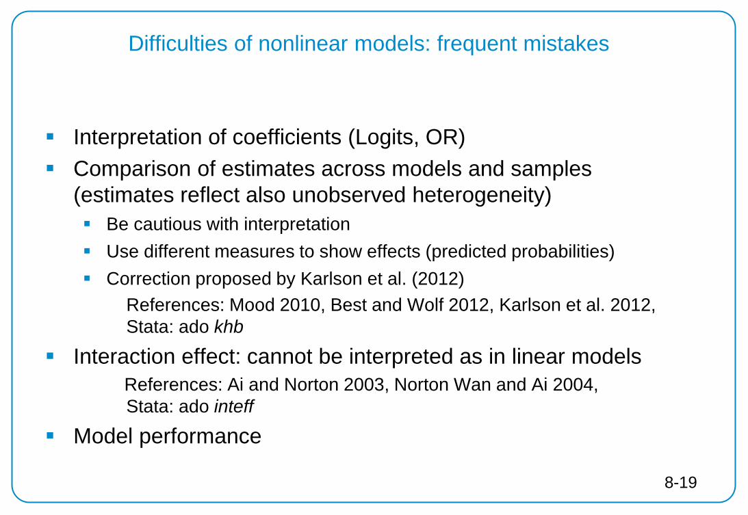
Difficulties of nonlinear models: frequent mistakes
Interpretation of coefficients (Logits, OR) Comparison of estimates across models and samples
(estimates reflect also unobserved heterogeneity) Be cautious with interpretation Use different measures to show effects (predicted probabilities) Correction proposed by Karlson et al. (2012)
References: Mood 2010, Best and Wolf 2012, Karlson et al. 2012, Stata: ado khb
Interaction effect: cannot be interpreted as in linear models References: Ai and Norton 2003, Norton Wan and Ai 2004,
Stata: ado inteff
Model performance
8-19
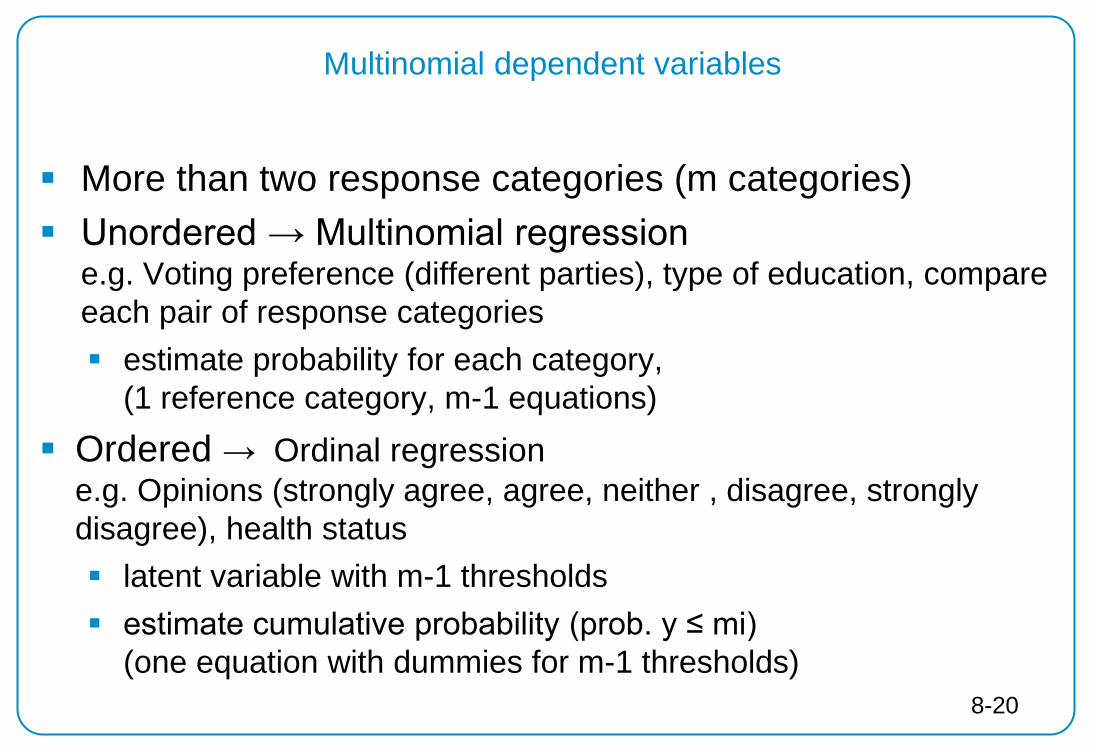
Multinomial dependent variables
More than two response categories (m categories) Unordered → Multinomial regression
e.g. Voting preference (different parties), type of education, compare each pair of response categories estimate probability for each category,
(1 reference category, m-1 equations) Ordered → Ordinal regression
e.g. Opinions (strongly agree, agree, neither , disagree, strongly disagree), health status latent variable with m-1 thresholds estimate cumulative probability (prob. y ≤ mi)
(one equation with dummies for m-1 thresholds) 8-20
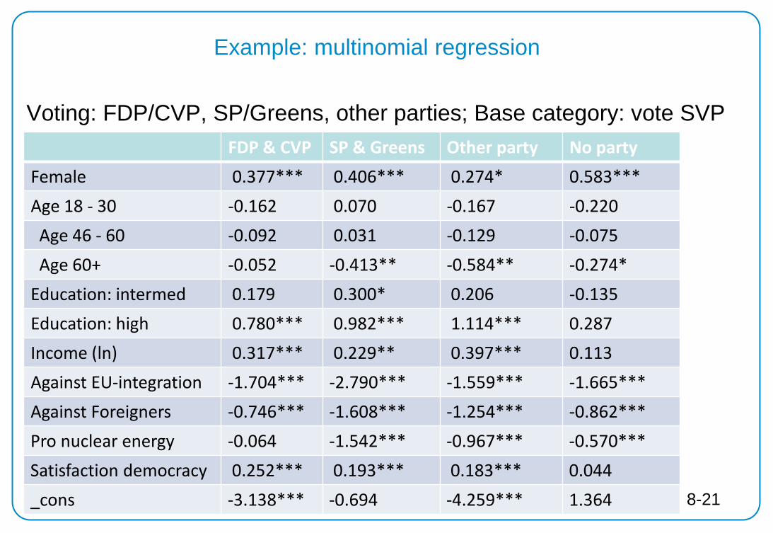
Example: multinomial regression
Voting: FDP/CVP, SP/Greens, other parties; Base category: vote SVP
FDP & CVP SP & Greens Other party No party Female 0.377*** 0.406*** 0.274* 0.583*** Age 18 - 30 -0.162 0.070 -0.167 -0.220 Age 46 - 60 -0.092 0.031 -0.129 -0.075 Age 60+ -0.052 -0.413** -0.584** -0.274* Education: intermed 0.179 0.300* 0.206 -0.135 Education: high 0.780*** 0.982*** 1.114*** 0.287 Income (ln) 0.317*** 0.229** 0.397*** 0.113 Against EU-integration -1.704*** -2.790*** -1.559*** -1.665*** Against Foreigners -0.746*** -1.608*** -1.254*** -0.862*** Pro nuclear energy -0.064 -1.542*** -0.967*** -0.570*** Satisfaction democracy 0.252*** 0.193*** 0.183*** 0.044 _cons -3.138*** -0.694 -4.259*** 1.364 8-21

Refresher: Panel data models in linear regression
Fixed effects models Yit= β1xi + β1xi +αi+ εit — αi: unobservable stable
individual characteristics (as variable, not residual)
— only variance within individuals taken into account
— Control for unobserved heterogeneity (consistent also if Cov(α,x)≠0) -> causal interpretation
— Effects of time-invariant characteristics cannot be estimated (e.g., sex, cohorts)
Random effect models Yit= α + β1xi + β1xi +αi+ εit —assumes α i ~ N(0,σα) —αi: unobservable stable
individual characteristics, part of residual
—Multilevel model with random intercepts
—Controls for unobserved heterogeneity (but consistent only if Cov(α,x)=0)
—Effects of time-invariant and time-varying covariates
22 8-22
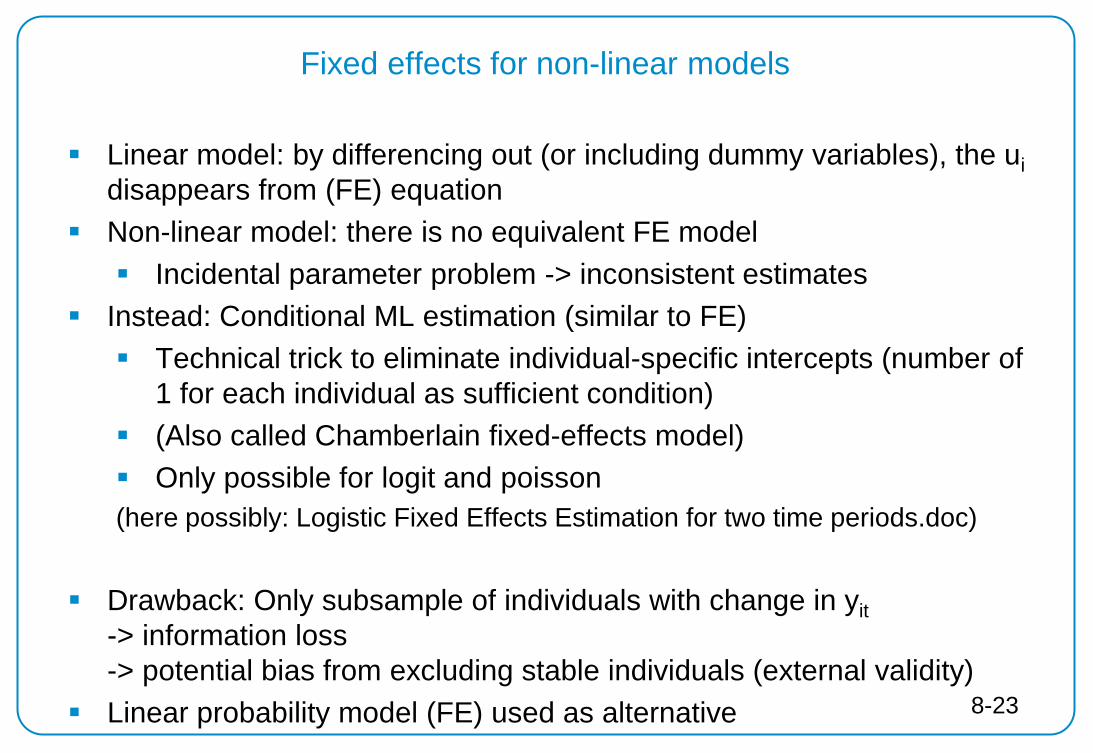
Fixed effects for non-linear models
Linear model: by differencing out (or including dummy variables), the ui disappears from (FE) equation
Non-linear model: there is no equivalent FE model Incidental parameter problem -> inconsistent estimates
Instead: Conditional ML estimation (similar to FE) Technical trick to eliminate individual-specific intercepts (number of
1 for each individual as sufficient condition) (Also called Chamberlain fixed-effects model) Only possible for logit and poisson (here possibly: Logistic Fixed Effects Estimation for two time periods.doc)
Drawback: Only subsample of individuals with change in yit
-> information loss -> potential bias from excluding stable individuals (external validity)
Linear probability model (FE) used as alternative 8-23
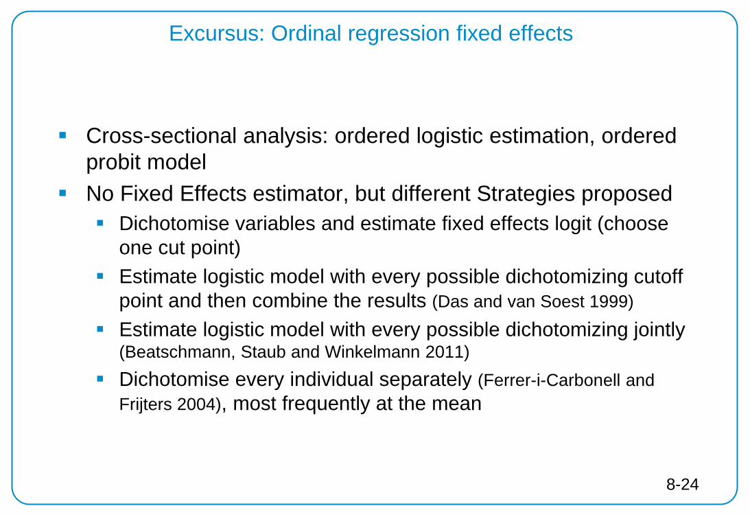
Excursus: Ordinal regression fixed effects
Cross-sectional analysis: ordered logistic estimation, ordered probit model
No Fixed Effects estimator, but different Strategies proposed Dichotomise variables and estimate fixed effects logit (choose
one cut point) Estimate logistic model with every possible dichotomizing cutoff
point and then combine the results (Das and van Soest 1999)
Estimate logistic model with every possible dichotomizing jointly (Beatschmann, Staub and Winkelmann 2011)
Dichotomise every individual separately (Ferrer-i-Carbonell and Frijters 2004), most frequently at the mean
8-24
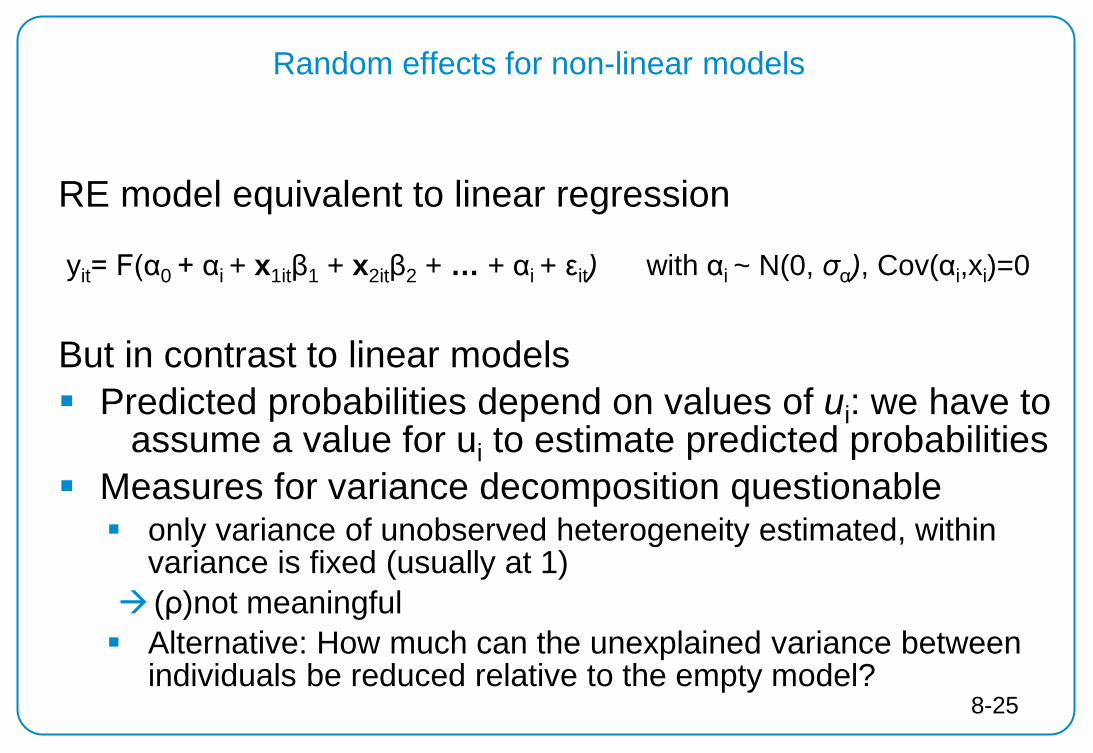
Random effects for non-linear models
RE model equivalent to linear regression yit= F(α0 + αi + x1itβ1 + x2itβ2 + … + αi + εit) with αi ~ N(0, σα), Cov(αi,xi)=0 But in contrast to linear models Predicted probabilities depend on values of ui: we have to
assume a value for ui to estimate predicted probabilities Measures for variance decomposition questionable only variance of unobserved heterogeneity estimated, within
variance is fixed (usually at 1) (ρ)not meaningful Alternative: How much can the unexplained variance between
individuals be reduced relative to the empty model? 8-25

Stata commands for non-linear panel models
Stata built-in commands —Random intercept models: xt prefix
xtlogit, xtprobit, xtpoisson, xttobit, xtcloglog, xtnbreg, xtologit —Random slope models: meqrlogit, meqrpoisson
Other software necessary for multinomial panel models (run from
Stata) —gllamm add-on (Rabe-Hesketh and Skrondal) to Stata (very powerful, freely available (but Stata necessary), slow,
become familiar with syntax) — runmlwin: command to run mlwin software from within Stata
(Mlwin software needs to be purchased) 8-26
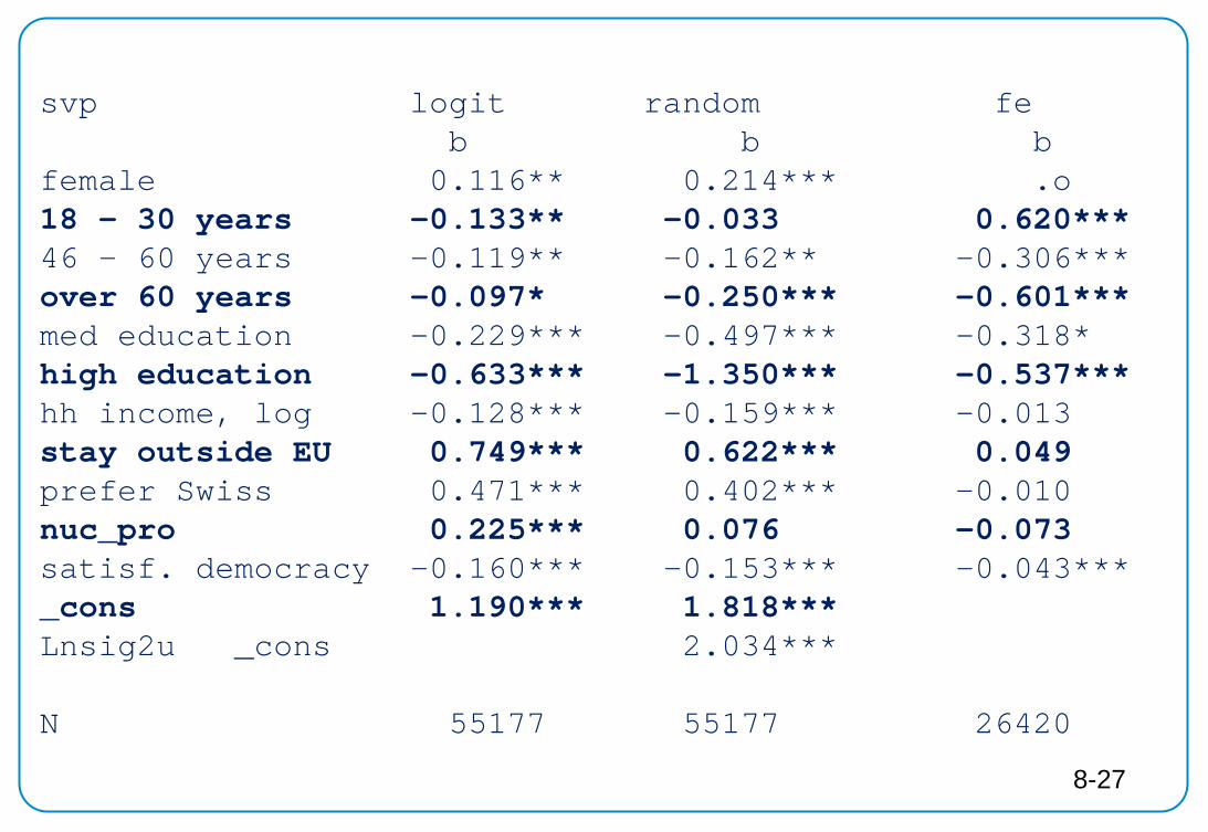
svp logit random fe b b b female 0.116** 0.214*** .o 18 - 30 years -0.133** -0.033 0.620*** 46 - 60 years -0.119** -0.162** -0.306*** over 60 years -0.097* -0.250*** -0.601*** med education -0.229*** -0.497*** -0.318* high education -0.633*** -1.350*** -0.537*** hh income, log -0.128*** -0.159*** -0.013 stay outside EU 0.749*** 0.622*** 0.049 prefer Swiss 0.471*** 0.402*** -0.010 nuc_pro 0.225*** 0.076 -0.073 satisf. democracy -0.160*** -0.153*** -0.043*** _cons 1.190*** 1.818*** Lnsig2u _cons 2.034*** N 55177 55177 26420
8-27

RE logistic model for event history analysis
Example for discrete event history analysis Dependent variable
0 event has not occurred 1 event has occurred (since last observation)
Independent variable Time until event occurrence Any other variable
Estimate logistic model or random effect logistic model
Example: change of vote intention (between parties)
Ind. Wave Vote intention, Party
Change between parties
Age
1 1 . . 23
1 2 A . 24
1 3 B 1 25
1 4 B 0 26
1 5 A 1 27
1 6 No party 0 28
Stata: xtlogit change age agesq 8-28
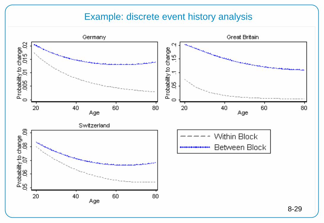
Example: discrete event history analysis
8-29