Introduction to Optimization...Introduction to Optimization, Marc Toussaint 3 1 Introduction Why...
89
Introduction to Optimization Marc Toussaint April 19, 2016 This is a direct concatenation and reformatting of all lecture slides and exercises from the Optimization course (summer term 2015, U Stuttgart), including indexing to help prepare for exams. Contents 1 Introduction 3 Types of optimization problems (1:3) 2 Unconstraint Optimization Basics 8 Plain gradient descent (2:1) Stepsize and step direction as core issues (2:2) Step- size adaptation (2:4) Backtracking (2:5) Line search (2:5) Wolfe conditions (2:7) Gra- dient descent convergence (2:8) Steepest descent direction (2:11) Covariant gradi- ent descent (2:13) Newton direction (2:14) Newton method (2:15) Gauss-Newton method (2:20) Quasi-Newton methods (2:23) Broyden-Fletcher-Goldfarb-Shanno (BFGS) (2:25) Conjugate gradient (2:28) Rprop (2:35) 3 Constrained Optimization 22 Constrained optimization (3:1) Log barrier method (3:6) Central path (3:9) Squared penalty method (3:12) Augmented Lagrangian method (3:14) Lagrangian: defini- tion (3:21) Lagrangian: relation to KKT (3:24) Karush-Kuhn-Tucker (KKT) conditions (3:25) Lagrangian: saddle point view (3:27) Lagrange dual problem (3:29) Log barrier as approximate KKT (3:33) Primal-dual interior-point Newton method (3:36) Phase I optimization (3:40) Trust region (3:41) 4 Convex Optimization 37 Function types: covex, quasi-convex, uni-modal (4:1) Linear program (LP) (4:6) Quadratic program (QP) (4:6) LP in standard form (4:7) Simplex method (4:11) LP- relaxations of integer programs (4:15) Sequential quadratic programming (4:23)
Transcript of Introduction to Optimization...Introduction to Optimization, Marc Toussaint 3 1 Introduction Why...

Introduction to Optimization
Marc Toussaint
April 19, 2016
This is a direct concatenation and reformatting of all lecture slides and exercises fromthe Optimization course (summer term 2015, U Stuttgart), including indexing to helpprepare for exams.
Contents
1 Introduction 3Types of optimization problems (1:3)
2 Unconstraint Optimization Basics 8Plain gradient descent (2:1) Stepsize and step direction as core issues (2:2) Step-size adaptation (2:4) Backtracking (2:5) Line search (2:5) Wolfe conditions (2:7) Gra-dient descent convergence (2:8) Steepest descent direction (2:11) Covariant gradi-ent descent (2:13) Newton direction (2:14) Newton method (2:15) Gauss-Newtonmethod (2:20) Quasi-Newton methods (2:23) Broyden-Fletcher-Goldfarb-Shanno(BFGS) (2:25) Conjugate gradient (2:28) Rprop (2:35)
3 Constrained Optimization 22Constrained optimization (3:1) Log barrier method (3:6) Central path (3:9) Squaredpenalty method (3:12) Augmented Lagrangian method (3:14) Lagrangian: defini-tion (3:21) Lagrangian: relation to KKT (3:24) Karush-Kuhn-Tucker (KKT) conditions(3:25) Lagrangian: saddle point view (3:27) Lagrange dual problem (3:29) Log barrieras approximate KKT (3:33) Primal-dual interior-point Newton method (3:36) Phase Ioptimization (3:40) Trust region (3:41)
4 Convex Optimization 37Function types: covex, quasi-convex, uni-modal (4:1) Linear program (LP) (4:6)Quadratic program (QP) (4:6) LP in standard form (4:7) Simplex method (4:11) LP-relaxations of integer programs (4:15) Sequential quadratic programming (4:23)
1
2 Introduction to Optimization, Marc Toussaint
5 Global & Bayesian Optimization 45Bandits (5:4) Exploration, Exploitation (5:6) Belief planning (5:8) Upper ConfidenceBound (UCB) (5:12) Global Optimization as infinite bandits (5:17) Gaussian Processesas belief (5:19) Expected Improvement (5:24) Maximal Probability of Improvement(5:24) GP-UCB (5:24)
6 Blackbox Optimization: Local, Stochastic & Model-based Search 55Blackbox optimization: definition (6:1) Blackbox optimization: overview (6:3)Greedy local search (6:5) Stochastic local search (6:6) Simulated annealing (6:7)Random restarts (6:10) Iterated local search (6:11) Variable neighborhood search(6:13) Coordinate search (6:14) Pattern search (6:15) Nelder-Mead simplex method(6:16) General stochastic search (6:20) Evolutionary algorithms (6:23) Covariance Ma-trix Adaptation (CMA) (6:24) Estimation of Distribution Algorithms (EDAs) (6:28)Model-based optimization (6:31) Implicit filtering (6:34)
7 Exercises 697.1 Exercise 1 . . . . . . . . . . . . . . . . . . . . . . . . . . . . . . . . . . . 697.2 Exercise 2 . . . . . . . . . . . . . . . . . . . . . . . . . . . . . . . . . . . 707.3 Exercise 3 . . . . . . . . . . . . . . . . . . . . . . . . . . . . . . . . . . . 717.4 Exercise 4 . . . . . . . . . . . . . . . . . . . . . . . . . . . . . . . . . . . 727.5 Exercise 6 . . . . . . . . . . . . . . . . . . . . . . . . . . . . . . . . . . . 737.6 Exercise 5 . . . . . . . . . . . . . . . . . . . . . . . . . . . . . . . . . . . 747.7 Exercise 6 . . . . . . . . . . . . . . . . . . . . . . . . . . . . . . . . . . . 757.8 Exercise 7 . . . . . . . . . . . . . . . . . . . . . . . . . . . . . . . . . . . 767.9 Exercise 7 . . . . . . . . . . . . . . . . . . . . . . . . . . . . . . . . . . . 777.10 Exercise 8 . . . . . . . . . . . . . . . . . . . . . . . . . . . . . . . . . . . 787.11 Exercise 8 . . . . . . . . . . . . . . . . . . . . . . . . . . . . . . . . . . . 797.12 Exercise 10 . . . . . . . . . . . . . . . . . . . . . . . . . . . . . . . . . . 797.13 Exercise 10 . . . . . . . . . . . . . . . . . . . . . . . . . . . . . . . . . . 807.14 Exercise 11 . . . . . . . . . . . . . . . . . . . . . . . . . . . . . . . . . . 80
8 Bullet points to help learning 828.1 Optimization Problems in General . . . . . . . . . . . . . . . . . . . . 828.2 Basic Unconstrained Optimization . . . . . . . . . . . . . . . . . . . . 828.3 Constrained Optimization . . . . . . . . . . . . . . . . . . . . . . . . . 848.4 Convex Optimization . . . . . . . . . . . . . . . . . . . . . . . . . . . . 858.5 Search methods for Blackbox optimization . . . . . . . . . . . . . . . 868.6 Bayesian Optimization . . . . . . . . . . . . . . . . . . . . . . . . . . . 86
Index 88

Introduction to Optimization, Marc Toussaint 3
1 Introduction
Why Optimization is interesting!
• In an otherwise unfortunate interview I’ve been asked why “we guys” (AI, ML, optimalcontrol people) always talk about optimality. “People are by no means optimal”, theinterviewer said. I think that statement pinpoints the whole misunderstanding of therole and concept of optimality principles.
– Optimality principles are a means of scientific (or engineering) description.– It is often easier to describe a thing (natural or artifical) via an optimality priciple
than directly
• Which science does not use optimality principles to describe nature & artifacts?– Physics, Chemistry, Biology, Mechanics, ...
– Operations research, scheduling, ...
– Computer Vision, Speach Recognition, Machine Learning, Robotics, ...
• Endless applications1:1
Teaching optimization
• Standard: Convex Optimization, Numerical Optimization• Discrete Optimization (Stefan Funke)• Exotics: Evolutionary Algorithms, Swarm optimization, etc
• In this lecture I try to cover the standard topics, but include as well work onstochastic search & global optimization
1:2
Rough Types of Optimization Problems
• Generic optimization problem:Let x ∈ Rn, f : Rn → R, g : Rn → Rm, h : Rn → Rl. Find
minx
f(x)
s.t. g(x) ≤ 0 , h(x) = 0
• Blackbox: only f(x) can be evaluated• Gradient: ∇f(x) can be evaluated• Gauss-Newton type: f(x) = φ(x)>φ(x) and∇φ(x) can be evaluated
• 2nd order: ∇2f(x) can be evaluated

4 Introduction to Optimization, Marc Toussaint
• “Approximate upgrade”:– Use samples of f(x) to approximate∇f(x) locally– Use samples of∇f(x) to approximate∇2f(x) locally
1:3
Optimization in Machine Learning: SVMs
• optimization problemmaxβ,||β||=1M subject to yi(φ(xi)
>β) ≥M, i = 1, . . . , n
• can be rephrased asminβ ||β|| subject to yi(φ(xi)
>β) ≥ 1, i = 1, . . . , n
Ridge regularization like ridge regression, but different loss
y
x
A
B
1:4
Optimization in Robotics
• Trajectories:Let xt ∈ Rn be a joint configuration and x = x1:T = (x1, . . . , xT ) a trajectory oflength T . Find
minx
T∑t=0
ft(xt−k:t)>ft(xt−k:t)
s.t. ∀t : gt(xt) ≤ 0 , ht(xt) = 0
(1)
• Control:
minu,q,λ
||u− a||2H (2)
s.t. u = Mq + h+ J>gλ (3)
Jφq = c (4)λ = λ∗ (5)

Introduction to Optimization, Marc Toussaint 5
Jg q = b (6)
1:5
Optimization in Computer Vision
• Andres Bruhn’s lectures• Flow estimation, (relaxed) min-cut problems, segmentation, ...
1:6
Planned Outline
• Unconstrained Optimization: Gradient- and 2nd order methods– stepsize & direction, plain gradient descent, steepest descent, line search & trust
region methods, conjugate gradient
– Newton, Gauss-Newton, Quasi-Newton, (L)BFGS• Constrained Optimization
– log barrier, squared penalties, augmented Lagrangian
– Lagrangian, KKT conditions, Lagrange dual, log barrier↔ approx. KKT• Special convex cases
– Linear Programming, (sequential) Quadratic Programming
– Simplex algorithm
– Relaxation of integer linear programs• Global Optimization
– infinite bandits, probabilistic modelling, exploration vs. exploitation, GP-UCB• Stochastic search
– Blackbox optimization (0th order methods), MCMC, downhill simplex
1:7
Books
6 Introduction to Optimization, Marc Toussaint
Boyd and Vandenberghe: Convex Opti-mization.http://www.stanford.edu/˜boyd/cvxbook/
(this course will not go to the full depth in math of Boyd et al.)1:8
Books
Nocedal & Wright: Numerical Optimiza-tionwww.bioinfo.org.cn/˜wangchao/maa/Numerical_Optimization.pdf
1:9
Organisation
• Webpage:http://ipvs.informatik.uni-stuttgart.de/mlr/marc/teaching/15-Optimization/
– Slides, Exercises & Software (C++)
– Links to books and other resources

Introduction to Optimization, Marc Toussaint 7
• Admin things, please first ask:Carola Stahl, [email protected], Raum 2.217
• Rules for the tutorials:– Doing the exercises is crucial!
– At the beginning of each tutorial:– sign into a list– mark which exercises you have (successfully) worked on
– Students are randomly selected to present their solutions
– You need 50% of completed exercises to be allowed to the exam
– Please check 2 weeks before the end of the term, if you can take the exam1:10

8 Introduction to Optimization, Marc Toussaint
2 Unconstraint Optimization Basics
Gradient descent
• Objective function: f : Rn → R
Gradient vector: ∇f(x) =[∂∂xf(x)
]>∈ Rn
• Problem:
minxf(x)
where we can evaluate f(x) and ∇f(x) for any x ∈ Rn
• Plain gradient descent: iterative steps in the direction −∇f(x).
Input: initial x ∈ Rn, function ∇f(x), stepsize α, tolerance θOutput: x
1: repeat2: x← x− α∇f(x)
3: until |∆x| < θ [perhaps for 10 iterations in sequence]
2:1
• Plain gradient descent is really not efficient• Two core issues of unconstrainted optimization:
A. StepsizeB. Descent direction
2:2
Stepsize
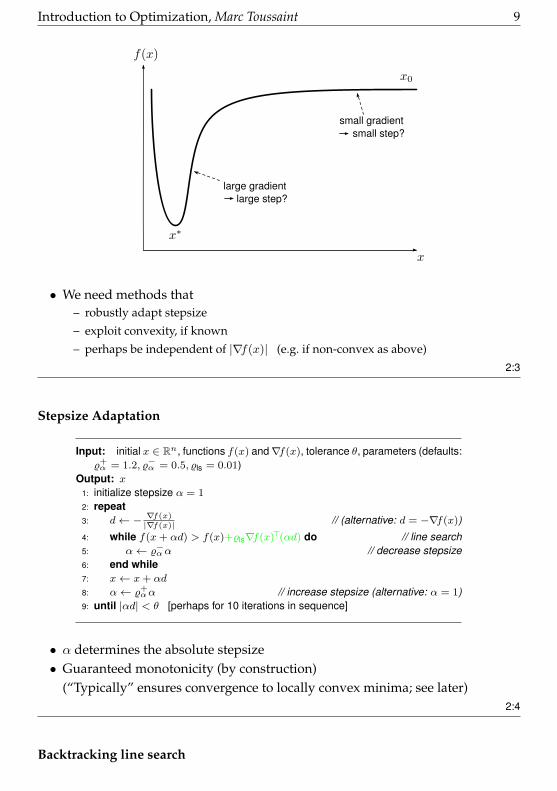
• Making steps proportional to∇f(x)?
Introduction to Optimization, Marc Toussaint 9
large gradient large step?
small gradient small step?
• We need methods that– robustly adapt stepsize
– exploit convexity, if known
– perhaps be independent of |∇f(x)| (e.g. if non-convex as above)2:3
Stepsize Adaptation
Input: initial x ∈ Rn, functions f(x) and∇f(x), tolerance θ, parameters (defaults:%+α = 1.2, %−α = 0.5, %ls = 0.01)
Output: x1: initialize stepsize α = 1
2: repeat3: d← − ∇f(x)
|∇f(x)| // (alternative: d = −∇f(x))
4: while f(x+ αd) > f(x)+%ls∇f(x)>(αd) do // line search5: α← %−αα // decrease stepsize6: end while7: x← x+ αd
8: α← %+αα // increase stepsize (alternative: α = 1)
9: until |αd| < θ [perhaps for 10 iterations in sequence]
• α determines the absolute stepsize• Guaranteed monotonicity (by construction)
(“Typically” ensures convergence to locally convex minima; see later)2:4
Backtracking line search

10 Introduction to Optimization, Marc Toussaint
• Line search in general denotes the problem
minα≥0
f(x+ αd)
for some step direction d.• The most common line search is backtracking, which decreases α as long as
f(x+ αd) > f(x) + %ls∇f(x)>(αd)
%−α describes the stepsize decrement in case of a rejected step%ls describes a minimum desired decrease in f(x)
• Boyd at al: typically %ls ∈ [0.01, 0.3] and %−α ∈ [0.1, 0.8]2:5
Backtracking line search
2:6
Wolfe Conditions
• The 1st Wolfe condition (“sufficient decrease condition”)
f(x+ αd) ≤ f(x)− %ls∇f(x)>(αd)
requires a decrease of f at least %ls-times “as expected”• The 2nd (stronger) Wolfe condition (“curvature condition”)
|∇f(x+ αd)>d| ≤ %ls2|∇f(x)>d|
implies a requires an decrease of the slope by a factor %ls2.%ls2 ∈ (%ls,
12 ) (for conjugate gradient)
• See Nocedal et al., Section 3.1 & 3.2 for more general proofs of convergence ofany method that ensures the Wolfe conditions after each line search
2:7
Introduction to Optimization, Marc Toussaint 11
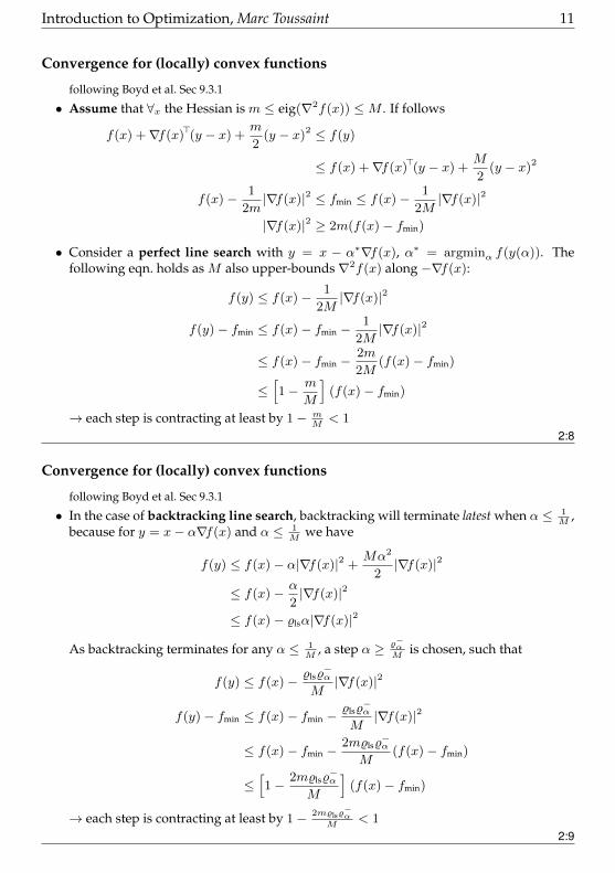
Convergence for (locally) convex functions
following Boyd et al. Sec 9.3.1
• Assume that ∀x the Hessian is m ≤ eig(∇2f(x)) ≤M . If follows
f(x) +∇f(x)>(y − x) + m
2(y − x)2 ≤ f(y)
≤ f(x) +∇f(x)>(y − x) + M
2(y − x)2
f(x)− 1
2m|∇f(x)|2 ≤ fmin ≤ f(x)−
1
2M|∇f(x)|2
|∇f(x)|2 ≥ 2m(f(x)− fmin)
• Consider a perfect line search with y = x − α∗∇f(x), α∗ = argminα f(y(α)). Thefollowing eqn. holds as M also upper-bounds∇2f(x) along −∇f(x):
f(y) ≤ f(x)− 1
2M|∇f(x)|2
f(y)− fmin ≤ f(x)− fmin −1
2M|∇f(x)|2
≤ f(x)− fmin −2m
2M(f(x)− fmin)
≤[1− m
M
](f(x)− fmin)
→ each step is contracting at least by 1− mM< 1
2:8
Convergence for (locally) convex functions
following Boyd et al. Sec 9.3.1
• In the case of backtracking line search, backtracking will terminate latest when α ≤ 1M
,because for y = x− α∇f(x) and α ≤ 1
Mwe have
f(y) ≤ f(x)− α|∇f(x)|2 +Mα2
2|∇f(x)|2
≤ f(x)− α
2|∇f(x)|2
≤ f(x)− %lsα|∇f(x)|2
As backtracking terminates for any α ≤ 1M
, a step α ≥ %−αM
is chosen, such that
f(y) ≤ f(x)− %ls%−α
M|∇f(x)|2
f(y)− fmin ≤ f(x)− fmin −%ls%−α
M|∇f(x)|2
≤ f(x)− fmin −2m%ls%
−α
M(f(x)− fmin)
≤[1− 2m%ls%
−α
M
](f(x)− fmin)
→ each step is contracting at least by 1− 2m%ls%−α
M< 1
2:9
12 Introduction to Optimization, Marc Toussaint
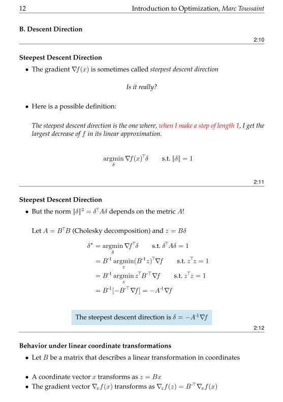
B. Descent Direction2:10
Steepest Descent Direction
• The gradient∇f(x) is sometimes called steepest descent direction
Is it really?
• Here is a possible definition:
The steepest descent direction is the one where, when I make a step of length 1, I get thelargest decrease of f in its linear approximation.
argminδ∇f(x)>δ s.t. ||δ|| = 1
2:11
Steepest Descent Direction
• But the norm ||δ||2 = δ>Aδ depends on the metric A!
Let A = B>B (Cholesky decomposition) and z = Bδ
δ∗ = argminδ∇f>δ s.t. δ>Aδ = 1
= B-1 argminz
(B-1z)>∇f s.t. z>z = 1
= B-1 argminz
z>B->∇f s.t. z>z = 1
= B-1[−B->∇f ] = −A-1∇f
The steepest descent direction is δ = −A-1∇f2:12
Behavior under linear coordinate transformations
• Let B be a matrix that describes a linear transformation in coordinates
• A coordinate vector x transforms as z = Bx
• The gradient vector∇xf(x) transforms as∇zf(z) = B->∇xf(x)

Introduction to Optimization, Marc Toussaint 13
• The metric A transforms as Az = B->AxB-1
• The steepest descent transforms as A-1z∇zf(z) = BA-1
x∇xf(x)
The steepest descent transforms like a normal coordinate vector (covariant)2:13
Newton Direction
• Assume we have access to the symmetric Hessian
∇2f(x) =
∂2
∂x1∂x1f(x) ∂2
∂x1∂x2f(x) · · · ∂2
∂x1∂xnf(x)
∂2
∂x1∂x2f(x)
......
...∂2
∂xn∂x1f(x) · · · · · · ∂2
∂xn∂xnf(x)
∈ Rn×n
• which defines the Taylor expansion:
f(x+ δ) ≈ f(x) +∇f(x)>δ +1
2δ>∇2f(x) δ
Note: ∇2f(x) acts like a metric for δ2:14
Newton method
• For finding roots (zero points) of f(x)
x← x− f(x)
f ′(x)
• For finding optima of f(x) in 1D:
x← x− f ′(x)
f ′′(x)
For x ∈ Rn:x← x−∇2f(x)-1∇f(x)
2:15

14 Introduction to Optimization, Marc Toussaint
Why 2nd order information is better
• Better direction:
Conjugate Gradient
Plain Gradient
2nd Order
• Better stepsize:– a full step jumps directly to the minimum of the local squared approx.
– often this is already a good heuristic
– additional stepsize reduction and dampening are straight-forward2:16
Newton method with adaptive stepsize
Input: initial x ∈ Rn, functions f(x),∇f(x),∇2f(x), tolerance θ, parameters(defaults: %+
α = 1.2, %−α = 0.5, %+λ = 1, %−λ = 0.5, %ls = 0.01)
Output: x1: initialize stepsize α = 1 and damping λ = λ0
2: repeat3: compute d to solve (∇2f(x) + λI) d = −∇f(x)
4: while f(x+ αd) > f(x) + %ls∇f(x)>(αd) do // line search5: α← %−αα // decrease stepsize6: optionally: λ← %+
λ λ and recompute d // increase damping7: end while8: x← x+ αd // step is accepted9: α← min{%+
αα, 1} // increase stepsize10: optionally: λ← %−λ λ // decrease damping11: until ||αd||∞ < θ
• Notes:
– Line 3 computes the Newton step d = −∇2f(x)-1∇f(x),use special Lapack routine dposv to solve Ax = b (using Cholesky)
– λ is called damping, related to trust region methods, makes the parabola more steeparound current xfor λ→∞: d becomes colinear with −∇f(x) but |d| = 0
2:17
Demo

Introduction to Optimization, Marc Toussaint 15
2:18
• In the remainder: Extensions of the Newton approach:– Gauss-Newton
– Quasi-Newton
– BFGS, (L)BFGS
– Conjugate Gradient
• And a crazy method: Rprop
• Postponed: trust region methods properly2:19
Gauss-Newton method
• Consider a sum-of-squares problem:
minxf(x) where f(x) = φ(x)>φ(x) =
∑i
φi(x)2
and we can evaluate φ(x), ∇φ(x) for any x ∈ Rn
• φ(x) ∈ Rd is a vector; each entry contributes a squared cost term to f(x)• ∇φ(x) is the Jacobian (d× n-matrix)
∇φ(x) =
∂∂x1
φ1(x)∂∂x2
φ1(x) · · · ∂∂xn
φ1(x)
∂∂x1
φ2(x)...
......
∂∂x1
φd(x) · · · · · · ∂∂xn
φd(x)
∈ Rd×n
with 1st-order Taylor expansion φ(x+ δ) = φ(x) +∇φ(x)δ2:20
Gauss-Newton method
• The gradient and Hessian of f(x) become
f(x) = φ(x)>φ(x)
∇f(x) = 2∇φ(x)>φ(x)
∇2f(x) = 2∇φ(x)>∇φ(x) + 2φ(x)>∇2φ(x)

16 Introduction to Optimization, Marc Toussaint
• The Gauss-Newton method is the Newton method for f(x) = φ(x)>φ(x) with approx-imating∇2φ(x) ≈ 0
In the Newton algorithm, replace line 3 by 3: compute d to solve (2∇φ(x)>∇φ(x) + λI) d = −2∇φ(x)>φ(x)
• The approximate Hessian 2∇φ(x)>∇φ(x) is always semi-pos-def!2:21
Quasi-Newton methods
2:22
Quasi-Newton methods
• Assume we cannot evaluate∇2f(x).Can we still use 2nd order methods?
• Yes: We can approximate ∇2f(x) from the data {(xi,∇f(xi))}ki=1 of previousiterations
2:23
Basic example
• We’ve seen already two data points (x1,∇f(x1)) and (x2,∇f(x2))
How can we estimate ∇2f(x)?
• In 1D:
∇2f(x) ≈ ∇f(x2)−∇f(x1)
x2 − x1
• In Rn: let y = ∇f(x2)−∇f(x1), δ = x2 − x1
∇2f(x) δ!= y δ
!= ∇2f(x)−1y
∇2f(x) =y y>
y>δ∇2f(x)−1 =
δδ>
δ>y
Convince yourself that the last line solves the desired relations[Left: how to update∇2f (x). Right: how to update directly∇2f(x)-1.]
2:24

Introduction to Optimization, Marc Toussaint 17
BFGS
• Broyden-Fletcher-Goldfarb-Shanno (BFGS) method:
Input: initial x ∈ Rn, functions f(x),∇f(x), tolerance θOutput: x
1: initialize H -1 = In2: repeat3: compute d = −H -1∇f(x)
4: perform a line search minα f(x+ αd)
5: δ ← αd
6: y ← ∇f(x+ δ)−∇f(x)
7: x← x+ δ
8: update H -1 ←(I− yδ>
δ>y
)>H -1(I− yδ>
δ>y
)+ δδ>
δ>y9: until ||δ||∞ < θ
• Notes:– The blue term is the H -1-update as on the previous slide– The red term “deletes” previous H -1-components
2:25
Quasi-Newton methods
• BFGS is the most popular of all Quasi-Newton methodsOthers exist, which differ in the exact H -1-update
• L-BFGS (limited memory BFGS) is a version which does not require to explic-itly store H -1 but instead stores the previous data {(xi,∇f(xi))}ki=1 and man-ages to compute d = −H -1∇f(x) directly from this data
• Some thought:In principle, there are alternative ways to estimateH -1 from the data {(xi, f(xi),∇f(xi))}ki=1,e.g. using Gaussian Process regression with derivative observations
– Not only the derivatives but also the value f(xi) should give information on H(x)for non-quadratic functions
– Should one weight ‘local’ data stronger than ‘far away’?(GP covariance function)
2:26
(Nonlinear) Conjugate Gradient
2:27
Conjugate Gradient
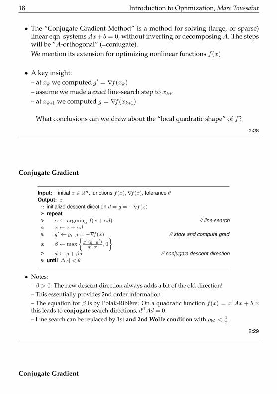
18 Introduction to Optimization, Marc Toussaint
• The “Conjugate Gradient Method” is a method for solving (large, or sparse)linear eqn. systems Ax+ b = 0, without inverting or decomposing A. The stepswill be “A-orthogonal” (=conjugate).We mention its extension for optimizing nonlinear functions f(x)
• A key insight:– at xk we computed g′ = ∇f(xk)
– assume we made a exact line-search step to xk+1
– at xk+1 we computed g = ∇f(xk+1)
What conclusions can we draw about the “local quadratic shape” of f?
2:28
Conjugate Gradient
Input: initial x ∈ Rn, functions f(x),∇f(x), tolerance θOutput: x
1: initialize descent direction d = g = −∇f(x)
2: repeat3: α← argminα f(x+ αd) // line search4: x← x+ αd
5: g′ ← g, g = −∇f(x) // store and compute grad
6: β ← max
{g>(g−g′)g′>g′
, 0
}7: d← g + βd // conjugate descent direction8: until |∆x| < θ
• Notes:– β > 0: The new descent direction always adds a bit of the old direction!– This essentially provides 2nd order information– The equation for β is by Polak-Ribiere: On a quadratic function f(x) = x>Ax + b>xthis leads to conjugate search directions, d′>Ad = 0.– Line search can be replaced by 1st and 2nd Wolfe condition with %ls2 <
12
2:29
Conjugate Gradient

Introduction to Optimization, Marc Toussaint 19
• For quadratic functions CG converges in n iterations. But each iteration doesline search
2:30
Convergence Rates Notes2:31
Convergence Rates Notes
• Linear, quadratic convergence (for q = 1, 2):
limk
|xk+1 − x∗||xk − x∗|p
= r
with rate r. E.g. xk = rk (linear) or xk+1 = rx2k (quadratic)
2:32
Convergence Rates Notes
• Theorem 3.3 in Nocedal et al.:Plain gradient descent with exact line search applied to f(x) = x>Ax, A witheigenvalues 0 < λ1 ≤ .. ≤ λn, satisfies
||xk+1 − x∗||2A ≤(λn − λ1
λn + λ1
)2
||xk − x∗||2A
• same on a smooth, locally pos-def function f(x): For sufficiently large k
f(xk+1)− f(x∗) ≤ r2[f(xk)− f(x∗)]
• Newton steps (with α = 1) on smooth locally pos-def function f(x):

20 Introduction to Optimization, Marc Toussaint
– xk converges quadratically to x∗
– |∇f(xk)| converges quadratically to zero
• Quasi-Newton methods also converge superlinearly if the Hessian approxima-tion is sufficiently precise (Thm. 3.7)
2:33
Rprop
2:34
Rprop
“Resilient Back Propagation” (outdated name from NN times...)
Input: initial x ∈ Rn, function f(x),∇f(x), initial stepsize α, tolerance θOutput: x
1: initialize x = x0, all αi = α, all gi = 0
2: repeat3: g ← ∇f(x)
4: x′ ← x
5: for i = 1 : n do6: if gig′i > 0 then // same direction as last time7: αi ← 1.2αi8: xi ← xi − αi sign(gi)
9: g′i ← gi10: else if gig′i < 0 then // change of direction11: αi ← 0.5αi12: xi ← xi − αi sign(gi)
13: g′i ← 0 // force last case next time14: else15: xi ← xi − αi sign(gi)
16: g′i ← gi17: end if18: optionally: cap αi ∈ [αmin xi, αmax xi]
19: end for20: until |x′ − x| < θ for 10 iterations in sequence
2:35
Rprop
• Rprop is a bit crazy:– stepsize adaptation in each dimension separately– it not only ignores |∇f | but also its exact direction
step directions may differ up to < 90◦ from∇f– Often works very robustly– Guarantees? See work by Ch. Igel
Introduction to Optimization, Marc Toussaint 21
• If you like, have a look at:Christian Igel, Marc Toussaint, W. Weishui (2005): Rprop using the natural gradientcompared to Levenberg-Marquardt optimization. In Trends and Applications in Con-structive Approximation. International Series of Numerical Mathematics, volume 151,259-272.
2:36
Appendix2:37
Stopping Criteria
• Standard references (Boyd) define stopping criteria based on the “change” inf(x), e.g. |∆f(x)| < θ or |∇f(x)| < θ.
• Throughout I will define stopping criteria based on the change in x, e.g. |∆x| <θ! In my experience with certain applications this is more meaningful, andinvariant of the scaling of f . But this is application dependent.
2:38
Evaluating optimization costs
• Standard references (Boyd) assume line search is cheap and measure optimiza-tion costs as the number of iterations (counting 1 per line search).
• Throughout I will assume that every evaluation of f(x) or (f(x),∇f(x)) or(f(x),∇f(x),∇2f(x)) is approx. equally expensive—as is the case in certain ap-plications.
2:39
22 Introduction to Optimization, Marc Toussaint
3 Constrained Optimization
Constrained Optimization
• General constrained optimization problem:Let x ∈ Rn, f : Rn → R, g : Rn → Rm, h : Rn → Rl find
minx
f(x) s.t. g(x) ≤ 0, h(x) = 0
In this lecture I’ll mostly focus on inequality constraints g, equality constraintsare analogous/easier
• Applications– Find an optimal, non-colliding trajectory in robotics– Optimize the shape of a turbine blade, s.t. it must not break– Optimize the train schedule, s.t. consistency/possibility
3:1
General approaches
• Try to somehow transform the constraint problem to
a series of unconstraint problems
a single but larger unconstraint problem
another constraint problem, hopefully simpler (dual, convex)3:2
General approaches
• Penalty & Barriers– Associate a (adaptive) penalty cost with violation of the constraint– Associate an additional “force compensating the gradient into the constraint” (aug-mented Lagrangian)– Associate a log barrier with a constraint, becoming ∞ for violation (interior pointmethod)
• Gradient projection methods (mostly for linear contraints)– For ‘active’ constraints, project the step direction to become tangantial– When checking a step, always pull it back to the feasible region

Introduction to Optimization, Marc Toussaint 23
• Lagrangian & dual methods– Rewrite the constrained problem into an unconstrained one– Or rewrite it as a (convex) dual problem
• Simplex methods (linear constraints)– Walk along the constraint boundaries
3:3
Barriers & Penalties
• Convention:
A barrier is really∞ for g(x) > 0
A penalty is zero for g(x) ≤ 0 and increases with g(x) > 0
3:4
Log barrier method or Interior Point method
3:5
Log barrier method
• Instead of
minx
f(x) s.t. g(x) ≤ 0
we address
minx
f(x)− µ∑i
log(−gi(x))
3:6

24 Introduction to Optimization, Marc Toussaint
Log barrier
• For µ→ 0, −µ log(−g) converges to∞[g > 0]
Notation: [boolean expression] ∈ {0, 1}
• The barrier gradient∇− log(−g) = ∇gg pushes away from the constraint
• Eventually we want to have a very small µ—but choosing small µ makes thebarrier very non-smooth, which might be bad for gradient and 2nd order meth-ods
3:7
Log barrier method
Input: initial x ∈ Rn, functions f(x), g(x),∇f(x),∇g(x), tolerance θ, parameters(defaults: %−µ = 0.5, µ0 = 1)
Output: x1: initialize µ = µ0
2: repeat3: find x← argminx f(x)− µ
∑i log(−gi(x)) with tolerance ∼10θ
4: decrease µ← %−µ µ
5: until |∆x| < θ
Note: See Boyd & Vandenberghe for alternative stopping criteria based on f precision(duality gap) and better choice of initial µ (which is called t there).
3:8
Central Path
• Every µ defines a different optimal x∗(µ)
x∗(µ) = argminx
f(x)− µ∑i
log(−gi(x))

Introduction to Optimization, Marc Toussaint 25
• Each point on the path can be understood as the optimal compromise of min-imizing f(x) and a repelling force of the constraints. (Which corresponds todual variables λ∗(µ).)
3:9
We will revisit the log barrier method later, once we introduced the Langrangian...3:10
Squared Penalty Method
3:11
Squared Penalty Method
• This is perhaps the simplest approach• Instead of
minx
f(x) s.t. g(x) ≤ 0
we address
minx
f(x) + µ
m∑i=1
[gi(x) > 0] gi(x)2
Input: initial x ∈ Rn, functions f(x), g(x),∇f(x),∇g(x), tol. θ, ε, parameters(defaults: %+
µ = 10, µ0 = 1)Output: x
1: initialize µ = µ0
2: repeat3: find x← argminx f(x) + µ
∑i[gi(x) > 0] gi(x)2 with tolerance ∼10θ
4: µ← %+µ µ
5: until |∆x| < θ and ∀i : gi(x) < ε
3:12
26 Introduction to Optimization, Marc Toussaint
Squared Penalty Method
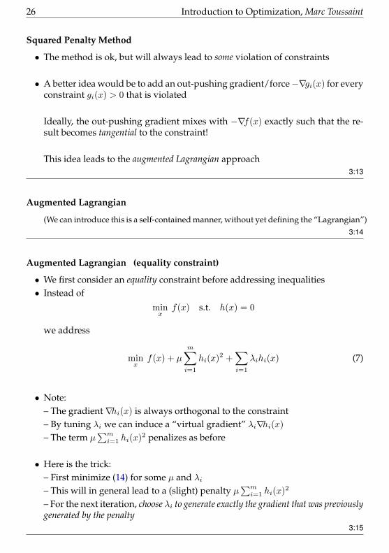
• The method is ok, but will always lead to some violation of constraints
• A better idea would be to add an out-pushing gradient/force−∇gi(x) for everyconstraint gi(x) > 0 that is violated
Ideally, the out-pushing gradient mixes with −∇f(x) exactly such that the re-sult becomes tangential to the constraint!
This idea leads to the augmented Lagrangian approach3:13
Augmented Lagrangian
(We can introduce this is a self-contained manner, without yet defining the “Lagrangian”)3:14
Augmented Lagrangian (equality constraint)
• We first consider an equality constraint before addressing inequalities• Instead of
minx
f(x) s.t. h(x) = 0
we address
minx
f(x) + µ
m∑i=1
hi(x)2 +∑i=1
λihi(x) (7)
• Note:– The gradient∇hi(x) is always orthogonal to the constraint– By tuning λi we can induce a “virtual gradient” λi∇hi(x)
– The term µ∑mi=1 hi(x)2 penalizes as before
• Here is the trick:– First minimize (14) for some µ and λi– This will in general lead to a (slight) penalty µ
∑mi=1 hi(x)2
– For the next iteration, choose λi to generate exactly the gradient that was previouslygenerated by the penalty
3:15
Introduction to Optimization, Marc Toussaint 27
• Optimality condition after an iteration:
x′ = argminx
f(x) + µ
m∑i=1
hi(x)2 +
m∑i=1
λihi(x)
⇒ 0 = ∇f(x′) + µ
m∑i=1
2hi(x′)∇hi(x′) +
m∑i=1
λi∇hi(x′)
• Update λ’s for the next iteration:∑i=1
λnewi ∇hi(x′) = µ
m∑i=1
2hi(x′)∇hi(x′) +
∑i=1
λoldi ∇hi(x′)
λnewi = λold
i + 2µhi(x′)
Input: initial x ∈ Rn, functions f(x), h(x),∇f(x),∇h(x), tol. θ, ε, parameters(defaults: %+
µ = 1, µ0 = 1)Output: x
1: initialize µ = µ0, λi = 0
2: repeat3: find x← argminx f(x) + µ
∑i hi(x)2 +
∑i λihi(x)
4: ∀i : λi ← λi + 2µhi(x′)
5: optionally, µ← %+µ µ
6: until |∆x| < θ and |hi(x)| < ε
3:16
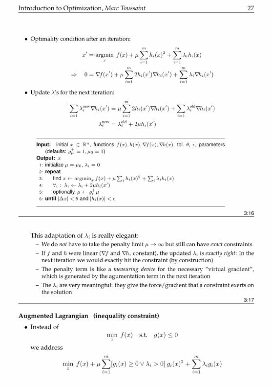
This adaptation of λi is really elegant:– We do not have to take the penalty limit µ→∞ but still can have exact constraints
– If f and h were linear (∇f and ∇hi constant), the updated λi is exactly right: In thenext iteration we would exactly hit the constraint (by construction)
– The penalty term is like a measuring device for the necessary “virtual gradient”,which is generated by the agumentation term in the next iteration
– The λi are very meaningful: they give the force/gradient that a constraint exerts onthe solution
3:17
Augmented Lagrangian (inequality constraint)
• Instead ofminx
f(x) s.t. g(x) ≤ 0
we address
minx
f(x) + µ
m∑i=1
[gi(x) ≥ 0 ∨ λi > 0] gi(x)2 +
m∑i=1
λigi(x)

28 Introduction to Optimization, Marc Toussaint
• A constraint is either active or inactive:– When active (gi(x) ≥ 0 ∨ λi > 0) we aim for equality gi(x) = 0
– When inactive (gi(x) < 0 ∧ λi = 0) we don’t penalize/augment– λi are zero or positive, but never negative
Input: initial x ∈ Rn, functions f(x), g(x),∇f(x),∇g(x), tol. θ, ε, parameters (defaults:%+µ = 1, µ0 = 1)
Output: x1: initialize µ = µ0, λi = 0
2: repeat3: find x← argminx f(x) + µ
∑i[gi(x) ≥ 0 ∨ λi > 0] gi(x)2 +
∑i λigi(x)
4: ∀i : λi ← max(λi + 2µgi(x′), 0)
5: optionally, µ← %+µµ
6: until |∆x| < θ and gi(x) < ε
3:18
• See also:M. Toussaint: A Novel Augmented Lagrangian Approach for Inequalities and Conver-gent Any-Time Non-Central Updates. e-Print arXiv:1412.4329, 2014.
3:19
The Lagrangian3:20
The Lagrangian
• Given a constraint problem
minx
f(x) s.t. g(x) ≤ 0
we define the Lagrangian as
L(x, λ) = f(x) +
m∑i=1
λigi(x)
• The λi ≥ 0 are called dual variables or Lagrange multipliers3:21
What’s the point of this definition?
• The Lagrangian is useful to compute optima analytically, on paper – that’s whyphysicist learn it early on

Introduction to Optimization, Marc Toussaint 29
• The Lagrangian implies the KKT conditions of optimality
• Optima are necessarily at saddle points of the Lagrangian
• The Lagrangian implies a dual problem, which is sometimes easier to solvethan the primal
3:22
Example: Some calculus using the Lagrangian
• For x ∈ R2, what is
minxx2 s.t. x1 + x2 = 1
• Solution:
L(x, λ) = x2 + λ(x1 + x2 − 1)
0 = ∇xL(x, λ) = 2x+ λ11
⇒ x1 = x2 = −λ/2
0 = ∇λL(x, λ) = x1 + x2 − 1 = −λ/2− λ/2− 1 ⇒ λ = −1
⇒x1 = x2 = 1/2
3:23
The “force” & KKT view on the Lagrangian
• At the optimum there must be a balance between the cost gradient −∇f(x) and thegradient of the active constraints −∇gi(x)
3:24

30 Introduction to Optimization, Marc Toussaint
The “force” & KKT view on the Lagrangian
• At the optimum there must be a balance between the cost gradient −∇f(x) and thegradient of the active constraints −∇gi(x)
• Formally: for optimal x: ∇f(x) ∈ span{∇gi(x)}
• Or: for optimal x there must exist λi such that −∇f(x) = −[∑
i(−λi∇gi(x))]
• For optimal x it must hold (necessary condition): ∃λ s.t.
∇f(x) +
m∑i=1
λi∇gi(x) = 0 (“stationarity”)
∀i : gi(x) ≤ 0 (primal feasibility)∀i : λi ≥ 0 (dual feasibility)
∀i : λigi(x) = 0 (complementary)
The last condition says that λi > 0 only for active constraints.These are the Karush-Kuhn-Tucker conditions (KKT, neglecting equality con-straints)
3:25
The “force” & KKT view on the Lagrangian
• The first condition (“stationarity”), ∃λ s.t.
∇f(x) +m∑i=1
λi∇gi(x) = 0
can be equivalently expressed as, ∃λ s.t.
∇xL(x, λ) = 0
• In that sense, the Lagrangian can be viewed as the “energy function” that gen-erates (for good choice of λ) the right balance between cost and constraint gra-dients
• This is exactly as in the augmented Lagrangian approach, where however we have anadditional (“augmented”) squared penalty that is used to tune the λi
3:26
Saddle point view on the Lagrangian
• Let’s briefly consider the equality case again:
minx
f(x) s.t. h(x) = 0

Introduction to Optimization, Marc Toussaint 31
with the Lagrangian
L(x, λ) = f(x) +
m∑i=1
λihi(x)
• Note:
minxL(x, λ) ⇒ 0 = ∇xL(x, λ) ↔ stationarity
maxλ
L(x, λ) ⇒ 0 = ∇λL(x, λ) = h(x) ↔ constraint
• Optima (x∗, λ∗) are saddle points where∇xL = 0 ensures stationarity and∇λL = 0 ensures the primal feasibility
3:27
Saddle point view on the Lagrangian
• In the inequality case:
maxλ≥0
L(x, λ) =
{f(x) if g(x) ≤ 0
∞ otherwise
λ = argmaxλ≥0
L(x, λ) ⇒
{λi = 0 if gi(x) < 0
0 = ∇λiL(x, λ) = gi(x) otherwise
This implies either (λi = 0∧gi(x) < 0) or gi(x) = 0, which is exactly equivalentto the complementarity and primal feasibility conditions• Again, optima (x∗, λ∗) are saddle points where
minx L enforces stationarity andmaxλ≥0 L enforces complementarity and primal feasibility
Together, minx L and maxλ≥0 L enforce the KKT conditions!3:28
The Lagrange dual problem
• Finding the saddle point can be written in two ways:
minx
maxλ≥0
L(x, λ) primal problem
maxλ≥0
minxL(x, λ) dual problem

32 Introduction to Optimization, Marc Toussaint
• Let’s define the Lagrange dual function as
l(λ) = minxL(x, λ)
Then we have
minxf(x) s.t. g(x) ≤ 0 primal problem
maxλ
l(λ) s.t. λ ≥ 0 dual problem
The dual problem is convex (objective=concave, constraints=convex), even ifthe primal is non-convex!
3:29
The Lagrange dual problem
• The dual function is always a lower bound (for any λi ≥ 0)
l(λ) = minxL(x, λ) ≤
[minxf(x) s.t. g(x) ≤ 0
]And consequently
maxλ≥0
minxL(x, λ) ≤ min
xmaxλ≥0
L(x, λ) = minx:g(x)≤0
f(x)
• We say strong duality holds iff
maxλ≥0
minxL(x, λ) = min
xmaxλ≥0
L(x, λ)
• If the primal is convex, and there exist an interior point
∃x : ∀i : gi(x) < 0
(which is called Slater condition), then we have strong duality3:30
And what about algorithms?
• So far we’ve only introduced a whole lot of formalism, and seen that the La-grangian sort of represents the constrained problem
• What are the algorithms we can get out of this?3:31
Log barrier method revisited3:32
Introduction to Optimization, Marc Toussaint 33
Log barrier method revisited
• Log barrier method: Instead of
minx
f(x) s.t. g(x) ≤ 0
we addressminx
f(x)− µ∑i
log(−gi(x))
• For given µ the optimality condition is
∇f(x)−∑i
µ
gi(x)∇gi(x) = 0
or equivalently
∇f(x) +∑i
λi∇gi(x) = 0 , λigi(x) = −µ
These are called modified (=approximate) KKT conditions.3:33
Log barrier method revisited
Centering (the unconstrained minimization) in the log barrier method is equivalent tosolving the modified KKT conditions.
Note also: On the central path, the duality gap is mµ:l(λ∗(µ)) = f(x∗(µ)) +
∑i λigi(x
∗(µ)) = f(x∗(µ))−mµ3:34
Primal-Dual interior-point Newton Method3:35
Primal-Dual interior-point Newton Method
• A core outcome of the Lagrangian theory was the shift in problem formulation:find x to minx f(x) s.t. g(x) ≤ 0
→ find x to solve the KKT conditions
Optimization problem −→ Solve KKT conditions

34 Introduction to Optimization, Marc Toussaint
• We think of the KKT conditions as an equation system r(x, λ) = 0, and can usethe Newton method for solving it:
∇r∆x∆λ
= −r
This leads to primal-dual algorithms that adapt x and λ concurrently. Roughly,this uses the curvature∇2f to estimate the right λ to push out of the constraint.
3:36
Primal-Dual interior-point Newton Method
• The first and last modified (=approximate) KKT conditions
∇f(x) +∑mi=1 λi∇gi(x) = 0 (“force balance”)∀i : gi(x) ≤ 0 (primal feasibility)∀i : λi ≥ 0 (dual feasibility)
∀i : λigi(x) = −µ (complementary)
can be written as the n+m-dimensional equation system
r(x, λ) = 0 , r(x, λ) := ∇f(x) +∇g(x)>λ−diag(λ)g(x)− µ1m
• Newton method to find the root r(x, λ) = 0
xλ
←xλ
−∇r(x, λ)-1r(x, λ)
∇r(x, λ) =∇2f(x) +
∑i λi∇2gi(x) ∇g(x)>
−diag(λ)∇g(x) −diag(g(x))
∈ R(n+m)×(n+m)
3:37
Primal-Dual interior-point Newton Method
• The method requires the Hessians∇2f(x) and ∇2gi(x)
– One can approximate the constraint Hessians∇2gi(x) ≈ 0
– Gauss-Newton case: f(x) = φ(x)>φ(x) only requires∇φ(x)
• This primal-dual method does a joint update of both– the solution x– the lagrange multipliers (constraint forces) λNo need for nested iterations, as with penalty/barrier methods!

Introduction to Optimization, Marc Toussaint 35
• The above formulation allows for a duality gap µ; choose µ = 0 or consult Boydhow to update on the fly (sec 11.7.3)
• The feasibility constraints gi(x) ≤ 0 and λi ≥ 0 need to be handled explicitlyby the root finder (the line search needs to ensure these constraints)
3:38
Phase I: Finding a feasible initialization3:39
Phase I: Finding a feasible initialization
• An elegant method for finding a feasible point x:
min(x,s)∈Rn+1
s s.t. ∀i : gi(x) ≤ s, s ≥ 0
or
min(x,s)∈Rn+m
m∑i=1
si s.t. ∀i : gi(x) ≤ si, si ≥ 0
3:40
Trust Region
• Instead of adapting the stepsize along a fixed direction, an alternative is toadapt the trust region• Rougly, while f(x+ δ) > f(x) + %ls∇f(x)>δ:
– Reduce trust region radius β
– try δ = argminδ:|δ|<β f(x+ δ) using a local quadratic model of f(x+ δ)
• The constraint optimization minδ:|δ|<β f(x+δ) can be translated into an uncon-strained minδ f(x+δ)+λδ2 for suitable λ. The λ is equivalent to a regularizationof the Hessian; see damped Newton.• We’ll not go into more details of trust region methods; see Nocedal Section 4.
3:41
General approaches
• Penalty & Barriers– Associate a (adaptive) penalty cost with violation of the constraint– Associate an additional “force compensating the gradient into the constraint” (aug-mented Lagrangian)– Associate a log barrier with a constraint, becoming ∞ for violation (interior pointmethod)

36 Introduction to Optimization, Marc Toussaint
• Gradient projection methods (mostly for linear contraints)– For ‘active’ constraints, project the step direction to become tangantial– When checking a step, always pull it back to the feasible region
• Lagrangian & dual methods– Rewrite the constrained problem into an unconstrained one– Or rewrite it as a (convex) dual problem
• Simplex methods (linear constraints)– Walk along the constraint boundaries
3:42

Introduction to Optimization, Marc Toussaint 37
4 Convex Optimization
Function types
• A function is defined convex iff
f(ax+ (1−a)y) ≤ a f(x) + (1−a) f(y)
for all x, y ∈ Rn and a ∈ [0, 1].
• A function is quasiconvex iff
f(ax+ (1−a)y) ≤ max{f(x), f(y)}
for any x, y ∈ Rm and a ∈ [0, 1]...alternatively, iff every sublevel set {x|f(x) ≤ α} is convex.
• [Subjective!] I call a function unimodal iff it has only 1 local minimum, whichis the global minimumNote: in dimensions n > 1 quasiconvexity is stronger than unimodality
• A general non-linear function is unconstrained and can have multiple localminima
4:1
convex ⊂ quasiconvex ⊂ unimodal ⊂ general4:2
Local optimization
• So far I avoided making explicit assumptions about problem convexity: Toemphasize that all methods we considered – except for Newton – are applicablealso on non-convex problems.
• The methods we considered are local optimization methods, which can be de-fined as– a method that adapts the solution locally– a method that is guaranteed to converge to a local minimum only
• Local methods are efficient– if the problem is (strictly) unimodal (strictly: no plateaux)– if time is critical and a local optimum is a sufficiently good solution– if the algorithm is restarted very often to hit multiple local optima
4:3
38 Introduction to Optimization, Marc Toussaint
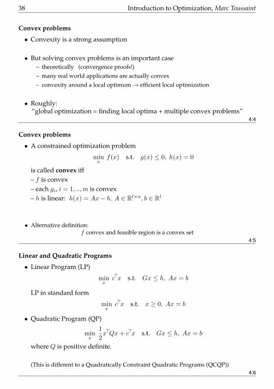
Convex problems
• Convexity is a strong assumption
• But solving convex problems is an important case– theoretically (convergence proofs!)
– many real world applications are actually convex
– convexity around a local optimum→ efficient local optimization
• Roughly:“global optimization = finding local optima + multiple convex problems”
4:4
Convex problems
• A constrained optimization problem
minx
f(x) s.t. g(x) ≤ 0, h(x) = 0
is called convex iff– f is convex– each gi, i = 1, ..,m is convex– h is linear: h(x) = Ax− b, A ∈ Rl×n, b ∈ Rl
• Alternative definition:f convex and feasible region is a convex set
4:5
Linear and Quadratic Programs
• Linear Program (LP)
minx
c>x s.t. Gx ≤ h, Ax = b
LP in standard form
minx
c>x s.t. x ≥ 0, Ax = b
• Quadratic Program (QP)
minx
1
2x>Qx+ c>x s.t. Gx ≤ h, Ax = b
where Q is positive definite.
(This is different to a Quadratically Constraint Quadratic Programs (QCQP))4:6

Introduction to Optimization, Marc Toussaint 39
Transforming an LP problem into standard form
• LP problem:minx
c>x s.t. Gx ≤ h, Ax = b
• Define slack variables:
minx,ξ
c>x s.t. Gx+ ξ = h, Ax = b, ξ ≥ 0
• Express x = x+ − x− with x+, x− ≥ 0:
minx+,x−,ξ
c>(x+ − x−)
s.t. G(x+ − x−) + ξ = h, A(x+ − x−) = b, ξ ≥ 0, x+ ≥ 0, x− ≥ 0
where (x+, x−, ξ) ∈ R2n+m
• Now this is conform with the standard form (replacing (x+, x−, ξ) ≡ x, etc)
minx
c>x s.t. x ≥ 0, Ax = b
4:7
Example LPs
Browse through the exercises 4.8-4.20 of Boyd & Vandenberghe!4:8
Linear Programming
– Algorithms– Application: LP relaxation of discret problems
4:9
Algorithms for Linear Programming
• All of which we know!– augmented Lagrangian (LANCELOT software), penalty– log barrier (“interior point method”, “[central] path following”)– primal-dual Newton

40 Introduction to Optimization, Marc Toussaint
• The simplex algorithm, walking on the constraints
(The emphasis in the notion of interior point methods is to distinguish fromconstraint walking methods.)
• Interior point and simplex methods are comparably efficientWhich is better depends on the problem
4:10
Simplex Algorithm
Georg Dantzig (1947)Note: Not to confuse with the Nelder–Mead method (downhill simplex method)
• We consider an LP in standard form
minx
c>x s.t. x ≥ 0, Ax = b
• Note that in a linear program the optimum is always situated at a corner
4:11
Simplex Algorithm

Introduction to Optimization, Marc Toussaint 41
• The Simplex Algorithm walks along the edges of the polytope, at every cornerchoosing the edge that decreases c>x most• This either terminates at a corner, or leads to an unconstrained edge (−∞ opti-
mum)
• In practise this procedure is done by “pivoting on the simplex tableaux”4:12
Simplex Algorithm
• The simplex algorithm is often efficient, but in worst case exponential in n andm.
• Interior point methods (log barrier) and, more recently again, augmented La-grangian methods have become somewhat more popular than the simplex al-gorithm
4:13
LP-relaxations of discrete problems4:14
Integer linear programming (ILP)
• An integer linear program (for simplicity binary) is
minx
c>x s.t. Ax = b, xi ∈ {0, 1}
• Examples:– Travelling Salesman: minxij
∑ij cijxij with xij ∈ {0, 1} and constraints ∀j :
∑i xij =
1 (columns sum to 1), ∀j :∑i xji = 1, ∀ij : tj − ti ≤ n − 1 + nxij (where ti are
additional integer variables).
– MaxSAT problem: In conjunctive normal form, each clause contributes an addi-tional variable and a term in the objective function; each clause contributes a con-straint
– Search the web for The Power of Semidefinite Programming Relaxations for MAXSAT4:15
LP relaxations of integer linear programs
• Instead of solving
minxc>x s.t. Ax = b, xi ∈ {0, 1}
we solveminxc>x s.t. Ax = b, x ∈ [0, 1]

42 Introduction to Optimization, Marc Toussaint
• Clearly, the relaxed solution will be a lower bound on the integer solution (some-times also called “outer bound” because [0, 1] ⊃ {0, 1})
• Computing the relaxed solution is interesting– as an “approximation” or initialization to the integer problem– to be aware of a lower bound– in cases where the optimal relaxed solution happens to be integer
4:16
Example: MAP inference in MRFs
• Given integer random variables xi, i = 1, .., n, a pairwise Markov RandomField (MRF) is defined as
f(x) =∑
(ij)∈E
fij(xi, xj) +∑i
fi(xi)
where E denotes the set of edges. Problem: find maxx f(x).(Note: any general (non-pairwise) MRF can be converted into a pair-wise one, blowing up thenumber of variables)
• Reformulate with indicator variables
bi(x) = [xi = x] , bij(x, y) = [xi = x] [xj = y]
These are nm+ |E|m2 binary variables• The indicator variables need to fulfil the constraints
bi(x), bij(x, y) ∈ {0, 1}∑x
bi(x) = 1 because xi takes eactly one value∑y
bij(x, y) = bi(x) consistency between indicators
4:17
Example: MAP inference in MRFs
• Finding maxx f(x) of a MRF is then equivalent to
maxbi(x),bij(x,y)
∑(ij)∈E
∑x,y
bij(x, y) fij(x, y) +∑i
∑x
bi(x) fi(x)
such that
bi(x), bij(x, y) ∈ {0, 1} ,∑x
bi(x) = 1 ,∑y
bij(x, y) = bi(x)

Introduction to Optimization, Marc Toussaint 43
• The LP-relaxation replaces the constraint to be
bi(x), bij(x, y) ∈ [0, 1] ,∑x
bi(x) = 1 ,∑y
bij(x, y) = bi(x)
This set of feasible b’s is called marginal polytope (because it describes thea space of “probability distributions” that are marginally consistent (but notnecessarily globally normalized!))
4:18
Example: MAP inference in MRFs
• Solving the original MAP problem is NP-hardSolving the LP-relaxation is really efficient
• If the solution of the LP-relaxation turns out to be integer, we’ve solved theoriginally NP-hard problem!If not, the relaxed problem can be discretized to be a good initialization fordiscrete optimization
• For binary attractive MRFs (a common case) the solution will always be integer4:19
Quadratic Programming
4:20
Quadratic Programming
minx
1
2x>Qx+ c>x s.t. Gx ≤ h, Ax = b
• Efficient Algorithms:– Interior point (log barrier)– Augmented Lagrangian– Penalty
• Highly relevant applications:– Support Vector Machines– Similar types of max-margin modelling methods
4:21

44 Introduction to Optimization, Marc Toussaint
Example: Support Vector Machine
• Primal:
maxβ,||β||=1
M s.t. ∀i : yi(φ(xi)>β) ≥M
• Dual:
minβ||β||2 s.t. ∀i : yi(φ(xi)
>β) ≥ 1
y
x
A
B
4:22
Sequential Quadratic Programming
• We considered general non-linear problems
minx
f(x) s.t. g(x) ≤ 0
where we can evaluate f(x), ∇f(x), ∇2f(x) and g(x), ∇g(x), ∇2g(x) for anyx ∈ Rn
→ Newton method
• In the unconstrained case, the standard step direction δ is (∇2f(x) + λI) δ =−∇f(x)
• In the constrained case, a natural step direction δ can be found by solving thelocal QP-approximation to the problem
minδ
f(x) +∇f(x)>δ + δ>∇2f(x)δ s.t. g(x) +∇g(x)>δ ≤ 0
This is an optimization problem over δ and only requires the evaluation off(x),∇f(x),∇2f(x), g(x),∇g(x) once.
4:23

Introduction to Optimization, Marc Toussaint 45
5 Global & Bayesian Optimization
Global Optimization
• Is there an optimal way to optimize (in the Blackbox case)?• Is there a way to find the global optimum instead of only local?
5:1
Outline
• Play a game
• Multi-armed bandits– Belief state & belief planning
– Upper Confidence Bound (UCB)
• Optimization as infinite bandits– GPs as belief state
• Standard heuristics:– Upper Confidence Bound (GP-UCB)
– Maximal Probability of Improvement (MPI)
– Expected Improvement (EI)5:2
Bandits5:3
Bandits
46 Introduction to Optimization, Marc Toussaint
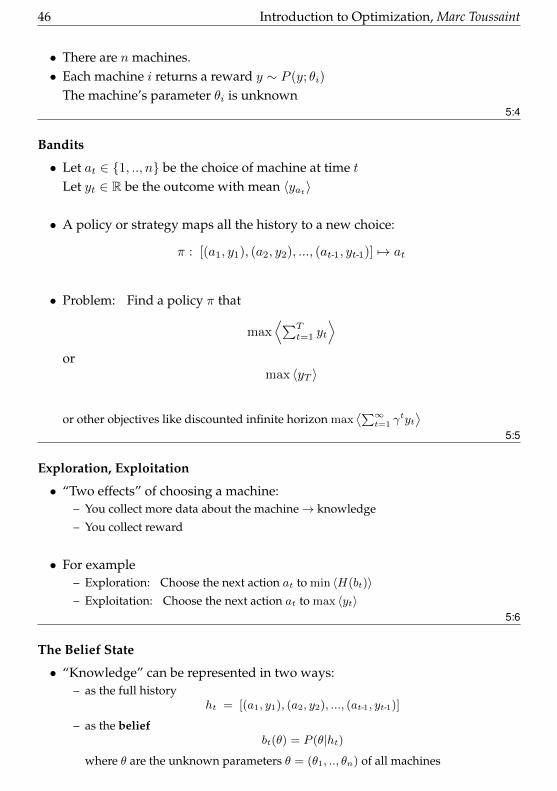
• There are n machines.• Each machine i returns a reward y ∼ P (y; θi)
The machine’s parameter θi is unknown5:4
Bandits
• Let at ∈ {1, .., n} be the choice of machine at time tLet yt ∈ R be the outcome with mean 〈yat〉
• A policy or strategy maps all the history to a new choice:
π : [(a1, y1), (a2, y2), ..., (at-1, yt-1)] 7→ at
• Problem: Find a policy π that
max⟨∑T
t=1 yt
⟩or
max 〈yT 〉
or other objectives like discounted infinite horizon max⟨∑∞
t=1 γtyt⟩
5:5
Exploration, Exploitation
• “Two effects” of choosing a machine:– You collect more data about the machine→ knowledge
– You collect reward
• For example– Exploration: Choose the next action at to min 〈H(bt)〉– Exploitation: Choose the next action at to max 〈yt〉
5:6
The Belief State
• “Knowledge” can be represented in two ways:– as the full history
ht = [(a1, y1), (a2, y2), ..., (at-1, yt-1)]
– as the beliefbt(θ) = P (θ|ht)
where θ are the unknown parameters θ = (θ1, .., θn) of all machines

Introduction to Optimization, Marc Toussaint 47
• In the bandit case:– The belief factorizes bt(θ) = P (θ|ht) =
∏i bt(θi|ht)
e.g. for Gaussian bandits with constant noise, θi = µi
bt(µi|ht) = N(µi|yi, si)
e.g. for binary bandits, θi = pi, with prior Beta(pi|α, β):
bt(pi|ht) = Beta(pi|α+ ai,t, β + bi,t)
ai,t =∑t−1s=1[as= i][ys=0] , bi,t =
∑t−1s=1[as= i][ys=1]
5:7
The Belief MDP
• The process can be modelled asa1 a2 a3y1 y2 y3
θ θ θ θ
or as Belief MDPa1 a2 a3y1 y2 y3
b0 b1 b2 b3
P (b′|y, a, b) =
{1 if b′ = b′[b,a,y]
0 otherwise, P (y|a, b) =
∫θab(θa) P (y|θa)
• The Belief MDP describes a different process: the interaction between the informationavailable to the agent (bt or ht) and its actions, where the agent uses his current belief toanticipate outcomes, P (y|a, b).
• The belief (or history ht) is all the information the agent has avaiable; P (y|a, b) the“best” possible anticipation of observations. If it acts optimally in the Belief MDP, it actsoptimally in the original problem.
Optimality in the Belief MDP ⇒ optimality in the original problem5:8
Optimal policies via Belief Planning
• The Belief MDP:a1 a2 a3y1 y2 y3
b0 b1 b2 b3
P (b′|y, a, b) =
{1 if b′ = b′[b,a,y]
0 otherwise, P (y|a, b) =
∫θab(θa) P (y|θa)

48 Introduction to Optimization, Marc Toussaint
• Belief Planning: Dynamic Programming on the value function
∀b : Vt-1(b) = maxπ
⟨∑Tt=t yt
⟩= max
π
[〈yt〉+
⟨∑Tt=t+1 yt
⟩ ]= max
at
∫ytP (yt|at, b)
[yt + Vt(b
′[b,at,yt]
)]
5:9
Optimal policies
• The value function assigns a value (maximal achievable return) to a state ofknowledge• The optimal policy is greedy w.r.t. the value function (in the sense of the maxat
above)• Computationally heavy: bt is a probability distribution, Vt a function over
probability distributions
• The term∫ytP (yt|at, bt-1)
[yt + Vt(bt-1[at, yt])
]is related to the Gittins Index: it can be computed
for each bandit separately.5:10
Example exercise
• Consider 3 binary bandits for T = 10.– The belief is 3 Beta distributions Beta(pi|α+ ai, β + bi) → 6 integers
– T = 10 → each integer ≤ 10
– Vt(bt) is a function over {0, .., 10}6
• Given a prior α = β = 1,a) compute the optimal value function and policy for the final reward and theaverage reward problems,b) compare with the UCB policy.
5:11
Greedy heuristic: Upper Confidence Bound (UCB)
1: Initializaiton: Play each machine once2: repeat3: Play the machine i that maximizes yi + β
√2 lnnni
4: until

Introduction to Optimization, Marc Toussaint 49
yi is the average reward of machine i so farni is how often machine i has been played so farn =
∑i ni is the number of rounds so far
β is often chosen as β = 1
See Finite-time analysis of the multiarmed bandit problem, Auer, Cesa-Bianchi & Fischer, Machinelearning, 2002.
5:12
UCB algorithms
• UCB algorithms determine a confidence interval such that
yi − σi < 〈yi〉 < yi + σi
with high probability.UCB chooses the upper bound of this confidence interval
• Optimism in the face of uncertainty
• Strong bounds on the regret (sub-optimality) of UCB (e.g. Auer et al.)5:13
Conclusions
• The bandit problem is an archetype for– Sequential decision making
– Decisions that influence knowledge as well as rewards/states
– Exploration/exploitation
• The same aspects are inherent also in global optimization, active learning & RL
• Belief Planning in principle gives the optimal solution
• Greedy Heuristics (UCB) are computationally much more efficient and guar-antee bounded regret
5:14
Further reading
• ICML 2011 Tutorial Introduction to Bandits: Algorithms and Theory, Jean-YvesAudibert, Remi Munos

50 Introduction to Optimization, Marc Toussaint
• Finite-time analysis of the multiarmed bandit problem, Auer, Cesa-Bianchi & Fis-cher, Machine learning, 2002.• On the Gittins Index for Multiarmed Bandits, Richard Weber, Annals of Applied
Probability, 1992.Optimal Value function is submodular.
5:15
Global Optimization
5:16
Global Optimization
• Let x ∈ Rn, f : Rn → R, find
minx
f(x)
(I neglect constraints g(x) ≤ 0 and h(x) = 0 here – but could be included.)
• Blackbox optimization: find optimium by sampling values yt = f(xt)
No access to∇f or∇2f
Observations may be noisy y ∼ N(y | f(xt), σ)5:17
Global Optimization = infinite bandits
• In global optimization f(x) defines a reward for every x ∈ Rn
– Instead of a finite number of actions at we now have xt
• Optimal Optimization could be defined as: find π : ht 7→ xt that
min⟨∑T
t=1 f(xt)⟩
ormin 〈f(xT )〉
5:18
Gaussian Processes as belief
• The unknown “world property” is the function θ = f
• Given a Gaussian Process prior GP (f |µ,C) over f and a history
Dt = [(x1, y1), (x2, y2), ..., (xt-1, yt-1)]

Introduction to Optimization, Marc Toussaint 51
the belief is
bt(f) = P (f |Dt) = GP(f |Dt, µ, C)
Mean(f(x)) = f(x) = κ(x)(K + σ2I)-1y response surface
Var(f(x)) = σ(x) = k(x, x)− κ(x)(K + σ2In)-1κ(x) confidence interval
• Side notes:– Don’t forget that Var(y∗|x∗, D) = σ2 + Var(f(x∗)|D)
– We can also handle discrete-valued functions f using GP classification5:19
5:20
Optimal optimization via belief planning
• As for bandits it holds
Vt-1(bt-1) = maxπ
⟨∑Tt=t yt
⟩= max
xt
∫ytP (yt|xt, bt-1)
[yt + Vt(bt-1[xt, yt])
]Vt-1(bt-1) is a function over the GP-belief!If we could compute Vt-1(bt-1) we “optimally optimize”
• I don’t know of a minimalistic case where this might be feasible5:21

52 Introduction to Optimization, Marc Toussaint
Conclusions
• Optimization as a problem of– Computation of the belief
– Belief planning
• Crucial in all of this: the prior P (f)
– GP prior: smoothness; but also limited: only local correlations!No “discovery” of non-local/structural correlations through the space
– The latter would require different priors, e.g. over different function classes5:22
Heuristics5:23
1-step heuristics based on GPs
• Maximize Probability of Improvement (MPI)
from Jones (2001)
xt = argmaxx
∫ y∗−∞N(y|f(x), σ(x))
• Maximize Expected Improvement (EI)
xt = argmaxx
∫ y∗−∞N(y|f(x), σ(x)) (y∗ − y)
• Maximize UCBxt = argmax
xf(x) + βtσ(x)
(Often, βt = 1 is chosen. UCB theory allows for better choices. See Srinivas et al. citation below.)5:24
Each step requires solving an optimization problem
• Note: each argmax on the previous slide is an optimization problem
• As f , σ are given analytically, we have gradients and Hessians. BUT: multi-modal problem.

Introduction to Optimization, Marc Toussaint 53
• In practice:– Many restarts of gradient/2nd-order optimization runs
– Restarts from a grid; from many random points
• We put a lot of effort into carefully selecting just the next query point5:25
From: Information-theoretic regret bounds for gaussian process optimization in the bandit setting Srinivas,Krause, Kakade & Seeger, Information Theory, 2012.
5:26

54 Introduction to Optimization, Marc Toussaint
5:27
Pitfall of this approach
• A real issue, in my view, is the choice of kernel (i.e. prior P (f))– ’small’ kernel: almost exhaustive search
– ’wide’ kernel: miss local optima
– adapting/choosing kernel online (with CV): might fail
– real f might be non-stationary
– non RBF kernels? Too strong prior, strange extrapolation
• Assuming that we have the right prior P (f) is really a strong assumption5:28
Further reading
• Classically, such methods are known as Kriging
• Information-theoretic regret bounds for gaussian process optimization in the banditsetting Srinivas, Krause, Kakade & Seeger, Information Theory, 2012.
• Efficient global optimization of expensive black-box functions. Jones, Schonlau, &Welch, Journal of Global Optimization, 1998.• A taxonomy of global optimization methods based on response surfaces Jones, Journal
of Global Optimization, 2001.• Explicit local models: Towards optimal optimization algorithms, Poland, Technical
Report No. IDSIA-09-04, 2004.5:29
Entropy Searchslides by Philipp Hennig
P. Hennig & C. Schuler: Entropy Search for Information-Efficient Global Optimiza-tion, JMLR 13 (2012).
5:30
Predictive Entropy Search
• Hernandez-Lobato, Hoffman & Ghahraman: Predictive Entropy Search for Effi-cient Global Optimization of Black-box Functions, NIPS 2014.• Also for constraints!• Code: https://github.com/HIPS/Spearmint/
5:31

Introduction to Optimization, Marc Toussaint 55
6 Blackbox Optimization: Local, Stochastic & Model-based Search
“Blackbox Optimization”
• We use the term to denote the problem: Let x ∈ Rn, f : Rn → R, find
minx
f(x)
where we can only evaluate f(x) for any x ∈ Rn
∇f(x) or ∇2f(x) are not (directly) accessible
• A constrained version: Let x ∈ Rn, f : Rn → R, g : Rn → {0, 1}, find
minx
f(x) s.t. g(x) = 1
where we can only evaluate f(x) and g(x) for any x ∈ Rn
I haven’t seen much work on this. Would be interesting to consider this more rigorously.6:1
“Blackbox Optimization” – terminology/subareas
• Stochastic Optimization (aka. Stochastic Search, Metaheuristics)– Simulated Annealing, Stochastic Hill Climing, Tabu Search
– Evolutionary Algorithms, esp. Evolution Strategies, Covariance Matrix Adaptation,Estimation of Distribution Algorithms
– Some of them (implicitly or explicitly) locally approximating gradients or 2nd ordermodels
• Derivative-Free Optimization (see Nocedal et al.)– Methods for (locally) convex/unimodal functions; extending gradient/2nd-order
methods
– Gradient estimation (finite differencing), model-based, Implicit Filtering
• Bayesian/Global Optimization– Methods for arbitrary (smooth) blackbox functions that get not stuck in local op-
tima.
– Very interesting domain – close analogies to (active) Machine Learning, bandits,POMDPs, optimal decision making/planning, optimal experimental design
6:2
Outline
• Basic downhill running– Greedy local search, stochastic local search, simulated annealing

56 Introduction to Optimization, Marc Toussaint
– Iterated local search, variable neighborhood search, Tabu search
– Coordinate & pattern search, Nelder-Mead downhill simplex
• Memorize or model something– General stochastic search
– Evolutionary Algorithms, Evolution Strategies, CMA, EDAs
– Model-based optimization, implicit filtering
• Bayesian/Global optimization: Learn & approximate optimal optimization– Belief planning view on optimal optimization
– GPs & Bayesian regression methods for belief tracking
– bandits, UBC, expected improvement, etc for decision making6:3
Basic downhill running– Greedy local search, stochastic local search, simulated annealing– Iterated local search, variable neighborhood search, Tabu search– Coordinate & pattern search, Nelder-Mead downhill simplex
6:4
Greedy local search (greedy downhill, hill climbing)
• Let x ∈ X be continuous or discrete• We assume there is a finite neighborhood N(x) ⊂ X defined for every x
• Greedy local search (variant 1):
Input: initial x, function f(x)
1: repeat2: x← argminy∈N(x) f(y) // convention: we assume x ∈ N(x)
3: until x converges
• Variant 2: x← the “first” y ∈ N(x) such that f(y) < f(x)
• Greedy downhill is a basic ingredient of discrete optimization• In the continuous case: what is N(x)? Why should it be fixed or finite?
6:5
Stochastic local search
• Let x ∈ Rn
• We assume a “neighborhood” probability distribution q(y|x), typically a Gaus-sian q(y|x) ∝ exp{− 1
2 (y − x)>Σ-1(y − x)}
Introduction to Optimization, Marc Toussaint 57
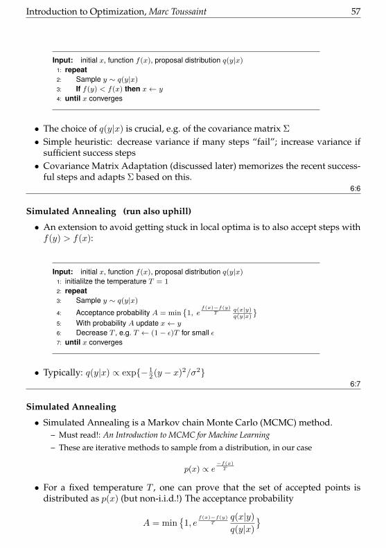
Input: initial x, function f(x), proposal distribution q(y|x)
1: repeat2: Sample y ∼ q(y|x)
3: If f(y) < f(x) then x← y
4: until x converges
• The choice of q(y|x) is crucial, e.g. of the covariance matrix Σ
• Simple heuristic: decrease variance if many steps “fail”; increase variance ifsufficient success steps• Covariance Matrix Adaptation (discussed later) memorizes the recent success-
ful steps and adapts Σ based on this.6:6
Simulated Annealing (run also uphill)
• An extension to avoid getting stuck in local optima is to also accept steps withf(y) > f(x):
Input: initial x, function f(x), proposal distribution q(y|x)
1: initialilze the temperature T = 1
2: repeat3: Sample y ∼ q(y|x)
4: Acceptance probability A = min{
1, ef(x)−f(y)
Tq(x|y)q(y|x)
}5: With probability A update x← y
6: Decrease T , e.g. T ← (1− ε)T for small ε7: until x converges
• Typically: q(y|x) ∝ exp{− 12 (y − x)2/σ2}
6:7
Simulated Annealing
• Simulated Annealing is a Markov chain Monte Carlo (MCMC) method.– Must read!: An Introduction to MCMC for Machine Learning– These are iterative methods to sample from a distribution, in our case
p(x) ∝ e−f(x)T
• For a fixed temperature T , one can prove that the set of accepted points isdistributed as p(x) (but non-i.i.d.!) The acceptance probability
A = min{
1, ef(x)−f(y)
Tq(x|y)
q(y|x)
}

58 Introduction to Optimization, Marc Toussaint
compares the f(y) and f(x), but also the reversibility of q(y|x)
• When cooling the temperature, samples focus at the extrema. Guaranteed tosample all extrema eventually• Of high theoretical relevance, less of practical
6:8
Simulated Annealing
6:9
Random Restarts (run downhill multiple times)
• Greedy local search is typically only used as an ingredient of more robust meth-ods• We assume to have a start distribution q(x)
• Random restarts:
1: repeat2: Sample x ∼ q(x)
3: x← GreedySearch(x) or StochasticSearch(x)
4: If f(x) < f(x∗) then x∗ ← x
5: until run out of budget
• Greedy local search requires a neighborhood function N(x)
Stochastic local search requires a transition proposal q(y|x)

Introduction to Optimization, Marc Toussaint 59
6:10
Iterated Local Search
• Random restarts may be rather expensive, sampling x ∼ q(x) is fully unin-formed• Iterated Local Search picks up the last visited local minimum x and restarts in
a meta-neighborhood N∗(x)
• Iterated Local Search (variant 1):
Input: initial x, function f(x)
1: repeat2: x← argminy′∈{GreedySearch(y) : y∈N∗(x)} f(y′)
3: until x converges
– This version evalutes a GreedySearch for all meta-neighbors y ∈ N∗(x) of the lastlocal optimum x
– The inner GreedySearch uses another neighborhood function N(x)
• Variant 2: x← the “first” y ∈ N∗(x) such that f(GS(y)) < f(x)
• Stochastic variant: Neighborhoods N(x) and N∗(x) are replaced by transitionproposals q(y|x) and q∗(y|x)
6:11
Iterated Local Search
• Application to Travelling Salesman Problem:k-opt neighbourhood: solutions which differ by at most k edges
from Hoos & Stutzle: Tutorial: Stochastic Search Algorithms
• GreedySearch uses 2-opt or 3-opt neighborhoodIterated Local Search uses 4-opt meta-neighborhood (double bridges)
6:12
Very briefly...
• Variable Neighborhood Search:

60 Introduction to Optimization, Marc Toussaint
– Switch the neighborhood function in different phases
– Similar to Iterated Local Search
• Tabu Search:– Maintain a tabu list points (or points features) which may not be visited again
– The list has a fixed finite size: FILO
– Intensification and diversification heuristics make it more global6:13
Coordinate Search
Input: Initial x ∈ Rn1: repeat2: for i = 1, .., n do3: α∗ = argminα f(x+ αei) // Line Search4: x← x+ α∗ei5: end for6: until x converges
• The LineSearch must be approximated– E.g. abort on any improvement, when f(x+ αei) < f(x)
– Remember the last successful stepsize αi for each coordinate
• Twiddle:
Input: Initial x ∈ Rn, initial stepsizes αi for all i = 1 : n
1: repeat2: for i = 1, .., n do3: x← argminy∈{x−αiei,x,x+αiei} f(y) // twiddle xi4: Increase αi if x changed; decrease αi otherwise5: end for6: until x converges
6:14
Pattern Search
– In each iteration k, have a (new) set of search directions Dk = {dki} and test stepsof length αk in these directions
– In each iteration, adapt the search directions Dk and step length αkDetails: See Nocedal et al.
6:15
Nelder-Mead method – Downhill Simplex Method

Introduction to Optimization, Marc Toussaint 61
6:16
Nelder-Mead method – Downhill Simplex Method
• Let x ∈ Rn
• Maintain n+ 1 points x0, .., xn, sorted by f(x0) < ... < f(xn)
• Compute center c of points• Reflect: y = c+ α(c− xn)
• If f(y) < f(x0): Expand: y = c+ γ(c− xn)
• If f(y) > f(xn-1): Contract: y = c+ %(c− xn)
• If still f(y) > f(xn): Shrink ∀i=1,..,nxi ← x0 + σ(xi − x0)
• Typical parameters: α = 1, γ = 2, % = − 12 , σ = 1
26:17
Summary: Basic downhill running
• These methods are highly relevant! Despite their simplicity• Essential ingredient to iterative approaches that try to find as many local min-
ima as possible
• Methods essentially differ in the notion ofneighborhood, transition proposal, or pattern of next search points
to consider• Iterated downhill can be very effective
62 Introduction to Optimization, Marc Toussaint
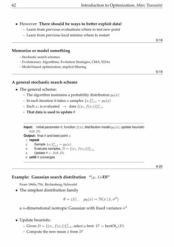
• However: There should be ways to better exploit data!– Learn from previous evaluations where to test new point
– Learn from previous local minima where to restart6:18
Memorize or model something– Stochastic search schemes– Evolutionary Algorithms, Evolution Strategies, CMA, EDAs– Model-based optimization, implicit filtering
6:19
A general stochastic search scheme
• The general scheme:– The algorithm maintains a probability distribution pθ(x)
– In each iteration it takes n samples {xi}ni=1 ∼ pθ(x)– Each xi is evaluated → data {(xi, f(xi))}ni=1
– That data is used to update θ
Input: initial parameter θ, function f(x), distribution model pθ(x), update heuristich(θ,D)
Output: final θ and best point x1: repeat2: Sample {xi}ni=1 ∼ pθ(x)
3: Evaluate samples, D = {(xi, f(xi))}ni=1
4: Update θ ← h(θ,D)
5: until θ converges
6:20
Example: Gaussian search distribution “(µ, λ)-ES”
From 1960s/70s. Rechenberg/Schwefel
• The simplest distribution family
θ = (x) , pθ(x) = N(x | x, σ2)
a n-dimenstional isotropic Gaussian with fixed variance σ2
• Update heuristic:– Given D = {(xi, f(xi))}λi=1, select µ best: D′ = bestOfµ(D)
– Compute the new mean x from D′
Introduction to Optimization, Marc Toussaint 63
• This algorithm is called “Evolution Strategy (µ, λ)-ES”– The Gaussian is meant to represent a “species”
– λ offspring are generated
– the best µ selected6:21
θ is the “knowledge/information” gained
• The parameter θ is the only “knowledge/information” that is being propagatedbetween iterationsθ encodes what has been learned from the historyθ defines where to search in the future
• The downhill methods of the previous section did not store any informationother than the current x. (Exception: Tabu search, Nelder-Mead)
• Evolutionary Algorithms are a special case of this stochastic search scheme6:22
Evolutionary Algorithms (EAs)
• EAs can well be described as special kinds of parameterizing pθ(x) and updat-ing θ
– The θ typically is a set of good points found so far (parents)
– Mutation & Crossover define pθ(x)
– The samples D are called offspring
– The θ-update is often a selection of the best, or “fitness-proportional” or rank-based
• Categories of EAs:– Evolution Strategies: x ∈ Rn, often Gaussian pθ(x)
– Genetic Algorithms: x ∈ {0, 1}n, crossover & mutation define pθ(x)
– Genetic Programming: x are programs/trees, crossover & mutation
– Estimation of Distribution Algorithms: θ directly defines pθ(x)6:23
Covariance Matrix Adaptation (CMA-ES)
• An obvious critique of the simple Evolution Strategies:– The search distribution N(x | x, σ2) is isotropic
(no going forward, no preferred direction)
– The variance σ is fixed!

64 Introduction to Optimization, Marc Toussaint
• Covariance Matrix Adaptation Evolution Strategy (CMA-ES)
6:24
Covariance Matrix Adaptation (CMA-ES)
• In Covariance Matrix Adaptation
θ = (x, σ, C, %σ, %C) , pθ(x) = N(x | x, σ2C)
where C is the covariance matrix of the search distribution• The θ maintains two more pieces of information: %σ and %C capture the “path”
(motion) of the mean x in recent iterations• Rough outline of the θ-update:
– Let D′ = bestOfµ(D) be the set of selected points
– Compute the new mean x from D′
– Update %σ and %C proportional to xk+1 − xk– Update σ depending on |%σ|– Update C depending on %c%>c (rank-1-update) and Var(D′)
6:25
CMA references
Hansen, N. (2006), ”The CMA evolution strategy: a comparing review”Hansen et al.: Evaluating the CMA Evolution Strategy on Multimodal TestFunctions, PPSN 2004.

Introduction to Optimization, Marc Toussaint 65
• For “large enough” populations local minima are avoided6:26
CMA conclusions
• It is a good starting point for an off-the-shelf blackbox algorithm• It includes components like estimating the local gradient (%σ, %C), the local
“Hessian” (Var(D′)), smoothing out local minima (large populations)6:27
Estimation of Distribution Algorithms (EDAs)
• Generally, EDAs fit the distribution pθ(x) to model the distribution of previ-ously good search pointsFor instance, if in all previous distributions, the 3rd bit equals the 7th bit, then the search distribu-tion pθ(x) should put higher probability on such candidates.pθ(x) is meant to capture the structure in previously good points, i.e. the dependencies/correlationbetween variables.
• A rather successful class of EDAs on discrete spaces uses graphical models tolearn the dependencies between variables, e.g.Bayesian Optimization Algorithm (BOA)
• In continuous domains, CMA is an example for an EDA6:28
Stochastic search conclusions
66 Introduction to Optimization, Marc Toussaint
Input: initial parameter θ, function f(x), distribution model pθ(x), update heuristich(θ,D)
Output: final θ and best point x1: repeat2: Sample {xi}ni=1 ∼ pθ(x)
3: Evaluate samples, D = {(xi, f(xi))}ni=1
4: Update θ ← h(θ,D)
5: until θ converges
• The framework is very general• The crucial difference between algorithms is their choice of pθ(x)
6:29
Model-based optimizationfollowing Nodecal et al. “Derivative-free optimization”
6:30
Model-based optimization
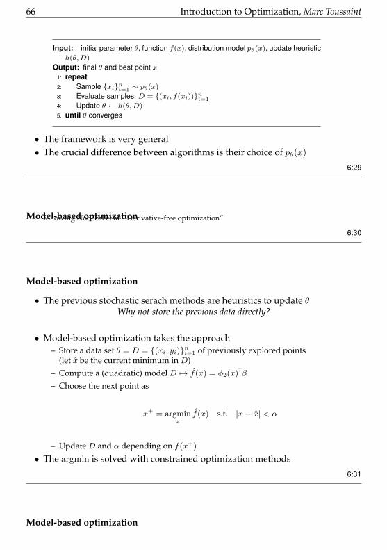
• The previous stochastic serach methods are heuristics to update θWhy not store the previous data directly?
• Model-based optimization takes the approach– Store a data set θ = D = {(xi, yi)}ni=1 of previously explored points
(let x be the current minimum in D)
– Compute a (quadratic) model D 7→ f(x) = φ2(x)>β
– Choose the next point as
x+ = argminx
f(x) s.t. |x− x| < α
– Update D and α depending on f(x+)
• The argmin is solved with constrained optimization methods
6:31
Model-based optimization
Introduction to Optimization, Marc Toussaint 67
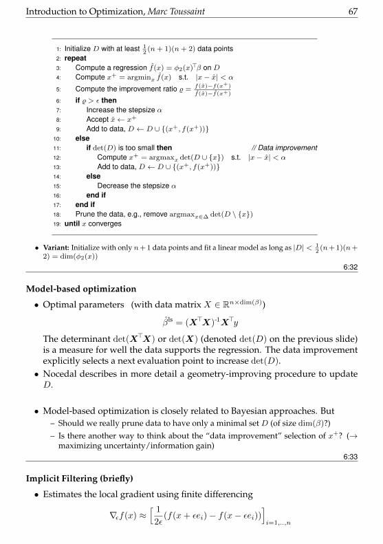
1: Initialize D with at least 12
(n+ 1)(n+ 2) data points2: repeat3: Compute a regression f(x) = φ2(x)>β on D4: Compute x+ = argminx f(x) s.t. |x− x| < α
5: Compute the improvement ratio % =f(x)−f(x+)
f(x)−f(x+)
6: if % > ε then7: Increase the stepsize α8: Accept x← x+
9: Add to data, D ← D ∪ {(x+, f(x+))}10: else11: if det(D) is too small then // Data improvement12: Compute x+ = argmaxx det(D ∪ {x}) s.t. |x− x| < α
13: Add to data, D ← D ∪ {(x+, f(x+))}14: else15: Decrease the stepsize α16: end if17: end if18: Prune the data, e.g., remove argmaxx∈∆ det(D \ {x})19: until x converges
• Variant: Initialize with only n+ 1 data points and fit a linear model as long as |D| < 12
(n+ 1)(n+2) = dim(φ2(x))
6:32
Model-based optimization
• Optimal parameters (with data matrix X ∈ Rn×dim(β))
βls = (X>X)-1X>y
The determinant det(X>X) or det(X) (denoted det(D) on the previous slide)is a measure for well the data supports the regression. The data improvementexplicitly selects a next evaluation point to increase det(D).• Nocedal describes in more detail a geometry-improving procedure to updateD.
• Model-based optimization is closely related to Bayesian approaches. But– Should we really prune data to have only a minimal set D (of size dim(β)?)
– Is there another way to think about the “data improvement” selection of x+? (→maximizing uncertainty/information gain)
6:33
Implicit Filtering (briefly)
• Estimates the local gradient using finite differencing
∇εf(x) ≈[ 1
2ε(f(x+ εei)− f(x− εei))
]i=1,..,n

68 Introduction to Optimization, Marc Toussaint
• Lines search along the gradient; if not succesful, decrease ε• Can be extended by using ∇εf(x) to update an approximation of the Hessian
(as in BFGS)6:34
Conclusions
• We covered– “downhill running”
– Two flavors of methods that exploit the recent data:– stochastic search (& EAs), maintaining θ that defines pθ(x)– model-based opt., maintaining local data D that defines f(x)
• These methods can be very efficient, but somehow the problem formalizationis unsatisfactory:
– What would be optimal optimization?
– What exactly is the information that we can gain from data about the optimum?
– If the optimization algorithm would be an “AI agent”, selecting points his actions,seeing f(x) his observations, what would be his optimal decision making strategy?
– And what about global blackbox optimization?6:35
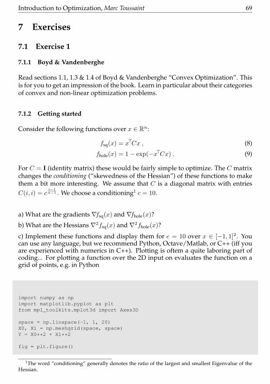
Introduction to Optimization, Marc Toussaint 69
7 Exercises
7.1 Exercise 1
7.1.1 Boyd & Vandenberghe
Read sections 1.1, 1.3 & 1.4 of Boyd & Vandenberghe “Convex Optimization”. Thisis for you to get an impression of the book. Learn in particular about their categoriesof convex and non-linear optimization problems.
7.1.2 Getting started
Consider the following functions over x ∈ Rn:
fsq(x) = x>Cx , (8)
fhole(x) = 1− exp(−x>Cx) . (9)
For C = I (identity matrix) these would be fairly simple to optimize. The C matrixchanges the conditioning (“skewedness of the Hessian”) of these functions to makethem a bit more interesting. We assume that C is a diagonal matrix with entriesC(i, i) = c
i−1n−1 . We choose a conditioning1 c = 10.
a) What are the gradients ∇fsq(x) and∇fhole(x)?
b) What are the Hessians∇2fsq(x) and ∇2fhole(x)?
c) Implement these functions and display them for c = 10 over x ∈ [−1, 1]2. Youcan use any language, but we recommend Python, Octave/Matlab, or C++ (iff youare experienced with numerics in C++). Plotting is oftem a quite laboring part ofcoding... For plotting a function over the 2D input on evaluates the function on agrid of points, e.g. in Python
import numpy as npimport matplotlib.pyplot as pltfrom mpl_toolkits.mplot3d import Axes3D
space = np.linspace(-1, 1, 20)X0, X1 = np.meshgrid(space, space)Y = X0**2 + X1**2
fig = plt.figure()
1The word “conditioning” generally denotes the ratio of the largest and smallest Eigenvalue of theHessian.

70 Introduction to Optimization, Marc Toussaint
ax = fig.add_subplot(111, projection=’3d’)ax.plot_wireframe(X0, X1, Y)plt.show()
Or in Octave:
[X0,X1] = meshgrid(linspace(-1,1,20),linspace(-1,1,20));Y = X0.**2 + X1.**2;mesh(X0,X1,Y);save ’datafile’ Y -ascii
Or you can store the grid data in a file and use gnuplot, e.g.:
splot [-1:1][-1:1] ’datafile’ matrix us ($1/10-1):($2/10-1):3 with lines
d) Implement a simple fixed stepsize gradient descent, iterating xk+1 = xk−α∇f(xk),with start point x0 = (1, 1), c = 10 and heuristically chosen α.
e) If you use Python or Octave, use an off-the-shelve optimization routine (ideallyIP-opt). In Python, scipy.optimize is a standard go-to solution for general optimiza-tion problems.
7.2 Exercise 2
7.2.1 Quadratics
Take the quadratic function fsq = x>Cxwith diagonal matrixC and entriesC(i, i) =λi.
a) Which 3 fundamental shapes does a 2-dimensional quadratic take? Plot the sur-face of fsq for various values of λ1, λ2 (big/small, positive/negative/zero). Couldyou predict these shapes before plotting them?
b) For which values of λ1, λ2 does minx fsq(x) not have a solution? For which doesit have infinite solutions? For which does it have exactly 1 solution? Find out empir-ically first, if you have to, then analytically.
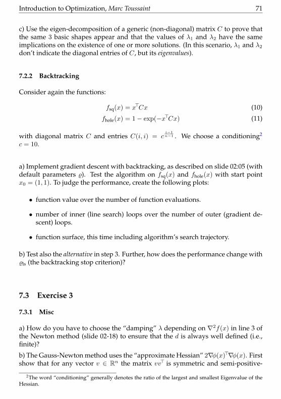
Introduction to Optimization, Marc Toussaint 71
c) Use the eigen-decomposition of a generic (non-diagonal) matrix C to prove thatthe same 3 basic shapes appear and that the values of λ1 and λ2 have the sameimplications on the existence of one or more solutions. (In this scenario, λ1 and λ2
don’t indicate the diagonal entries of C, but its eigenvalues).
7.2.2 Backtracking
Consider again the functions:
fsq(x) = x>Cx (10)
fhole(x) = 1− exp(−x>Cx) (11)
with diagonal matrix C and entries C(i, i) = ci−1n−1 . We choose a conditioning2
c = 10.
a) Implement gradient descent with backtracking, as described on slide 02:05 (withdefault parameters %). Test the algorithm on fsq(x) and fhole(x) with start pointx0 = (1, 1). To judge the performance, create the following plots:
• function value over the number of function evaluations.
• number of inner (line search) loops over the number of outer (gradient de-scent) loops.
• function surface, this time including algorithm’s search trajectory.
b) Test also the alternative in step 3. Further, how does the performance change with%ls (the backtracking stop criterion)?
7.3 Exercise 3
7.3.1 Misc
a) How do you have to choose the “damping” λ depending on ∇2f(x) in line 3 ofthe Newton method (slide 02-18) to ensure that the d is always well defined (i.e.,finite)?
b) The Gauss-Newton method uses the “approximate Hessian” 2∇φ(x)>∇φ(x). Firstshow that for any vector v ∈ Rn the matrix vv> is symmetric and semi-positive-
2The word “conditioning” generally denotes the ratio of the largest and smallest Eigenvalue of theHessian.

72 Introduction to Optimization, Marc Toussaint
definite.3 From this, how can you argue that ∇φ(x)>∇φ(x) is also symmetric andsemi-positive-definite?
c) In the context of BFGS, convince yourself that choosing H -1 = δδ>
δ>yindeed fulfills
the desired relation δ = H -1y, where δ and y are defined as on slide 02-23. Are thereother choices of H -1 that fulfill the relation? Which?
7.3.2 Gauss-Newton
In x ∈ R2 consider the function
f(x) = φ(x)>φ(x) , φ(x) =
sin(ax1)sin(acx2)
2x1
2cx2
The function is plotted above for a = 4 (left) and a = 5 (right, having local minima),and conditioning c = 1. The function is non-convex.
a) Extend your backtracking method implemented in the last week’s exercise to aGauss-Newton method (with constant λ) to solve the unconstrained minimizationproblem minx f(x) for a random start point in x ∈ [−1, 1]2. Compare the algorithmfor a = 4 and a = 5 and conditioning c = 3 with gradient descent.
b) Optimize the function using your optimization library of choice (If you can, usea BFGS implementation.)
7.4 Exercise 4
7.4.1 Alternative Barriers & Penalties
Propose 3 alternative barrier functions, and 3 alternative penalty functions. To dis-play functions, gnuplot is useful, e.g., plot -log(-x).
3 A matrix A ∈ Rn×n is semi-positive-definite simply when for any x ∈ Rn it holds x>Ax ≥ 0.Intuitively: A might be a metric as it “measures” the norm of any x as positive. Or: If A is a Hessian,the function is (locally) convex.

Introduction to Optimization, Marc Toussaint 73
7.4.2 Squared Penalties & Log Barriers
In a previous exercise we defined the “hole function” f chole(x), where we now as-sume a conditioning c = 4.
Consider the optimization problem
minxf chole(x) s.t. g(x) ≤ 0 (12)
g(x) = x>x− 1xn + 1/c
(13)
a) First, assume n = 2 (x ∈ R2 is 2-dimensional), c = 4, and draw on paper whatthe problem looks like and where you expect the optimum.
b) Implement the Squared Penalty Method. (In the inner loop you may choose anymethod, including simple gradient methods.) Choose as a start point x = ( 1
2 ,12 ).
Plot its optimization path and report on the number of total function/gradient eval-uations needed.
c) Test the scaling of the method for n = 10 dimensions.
d) Implement the Log Barrier Method and test as in b) and c). Compare the func-tion/gradient evaluations needed.
7.5 Exercise 6
7.5.1 Min-max 6= max-min
Give a function f(x, y) such that
maxy
minxf(x, y) 6= min
xmaxy
f(x, y)
7.5.2 Primal-dual Newton method
Slide 03:38 describes the primal-dual Newton method. Implement it to solve thesame constrained problem we considered in the last exercise.
a) d = −∇r(x, λ)-1r(x, λ) defines the search direction. Ideally one can make a stepwith factor α = 1 in this direction. However, line search needs to ensure (i) dualfeasibility λ > 0, (ii) primal feasibility g(x) ≤ 0, and (iii) sufficient decrease (theWolfe condition). Line search decreases the step factor α to ensure these conditions(in this order), where the Wolfe condition here reads
|r(z + αd)| ≤ (1− %lsα)|r(z)| , z =xλ
74 Introduction to Optimization, Marc Toussaint
b) Initialize µ = 1. In each iteration decrease it by some factor.
c) Optionally, regularize ∇r(x, λ) to robustify inversion.
7.5.3 Maybe skip: Phase I & Log Barriers
Consider the the same problem 14.
a) Use the method you implemented above to find a feasible initialization (Phase I).Do this by solving the n+ 1-dimensional problem
min(x,s)∈Rn+1
s s.t. ∀i : gi(x) ≤ s, s ≥ −ε
For some very small ε. Initialize this with the infeasible point (1, 1) ∈ R2.
b) Once you’ve found a feasible point, use the standard log barrier method to findthe solution to the original problem (14). Start with µ = 1, and decrease it byµ← µ/2 in each iteration. In each iteration also report λi := µ
gi(x) for i = 1, 2.
7.6 Exercise 5
7.6.1 Equality Constraint Penalties and augmented Lagrangian
Take a squared penalty approach to solving a constrained optimization problem
minx
f(x) + µ
m∑i=1
hi(x)2 (14)
The Augmented Lagrangian method adds yet another penalty term
minx
f(x) + µ
m∑i=1
hi(x)2 +
m∑i=1
λihi(x) (15)
Assume that if we minimize (14) we end up at a solution x for which each hi(x)is reasonable small, but not exactly zero. Prove, in the context of the AugmentedLagrangian method, that setting λi = 2µhi(x) will, if we assume that the gradients∇f(x) and ∇h(x) are (locally) constant, ensure that the minimum of (15) fulfills theconstraints h(x) = 0.
Tip: Think intuitive. Think about how the gradient that arises from the penalty in(14) is now generated via the λi.

Introduction to Optimization, Marc Toussaint 75
7.6.2 Lagrangian and dual function
(Taken roughly from ‘Convex Optimization’, Ex. 5.1)
A simple example. Consider the optimization problem
minx2 + 1 s.t. (x− 2)(x− 4) ≤ 0
with variable x ∈ R.
a) Derive the optimal solution x∗ and the optimal value p∗ = f(x∗) by hand.
b) Write down the Lagrangian L(x, λ). Plot (using gnuplot or so) L(x, λ) over x forvarious values of λ ≥ 0. Verify the lower bound property minx L(x, λ) ≤ p∗, wherep∗ is the optimum value of the primal problem.
c) Derive the dual function l(λ) = minx L(x, λ) and plot it (for λ ≥ 0). Derive thedual optimal solution λ∗ = argmaxλ l(λ). Is maxλ l(λ) = p∗ (strong duality)?
7.6.3 Augmented Lagrangian Programming
Take last week’s programming exercise on Squared Penalty and “augment” it sothat it becomes the Augmented Lagrangian method. Compare the function/gradientevaluations between the simple Squared Penalty method and the Augmented method.
7.7 Exercise 6
7.7.1 Min-max 6= max-min
Give a function f(x, y) such that
maxy
minxf(x, y) 6= min
xmaxy
f(x, y)
7.7.2 Lagrangian Method of Multipliers
We have previously defined the “hole function” as f chole(x) = 1 − exp(−x>Cx),where C is a n × n diagonal matrix with Cii = c
i−1n−1 . Assume conditioning c =
10 and use the Lagrangian Method of Multipliers to solve on paper the followingconstrained optimization problem in 2D.
minxf chole(x) s.t. h(x) = 0 (16)
h(x) = v>x− 1 (17)
Near the very end, you won’t be able to proceed until you have special values forv. Go as far as you can without the need for these values.
76 Introduction to Optimization, Marc Toussaint
7.7.3 Primal-dual Newton method
Slide 03:38 describes the primal-dual Newton method. Implement it to solve thesame constrained problem we considered in the last exercise.
a) d = −∇r(x, λ)-1r(x, λ) defines the search direction. Ideally one can make a stepwith factor α = 1 in this direction. However, line search needs to ensure (i) dualfeasibility λ > 0, (ii) primal feasibility g(x) ≤ 0, and (iii) sufficient decrease (theWolfe condition). Line search decreases the step factor α to ensure these conditions(in this order), where the Wolfe condition here reads
|r(z + αd)| ≤ (1− %lsα)|r(z)| , z =xλ
b) Initialize µ = 1. In each iteration decrease it by some factor.
c) Optionally, regularize∇r(x, λ) to robustify inversion.
7.8 Exercise 7
Solving real-world problems involves 2 subproblems:
1) formulating the problem as an optimization problem (conform to a standardoptimization problem category) (→ human)
2) the actual optimization problem (→ algorithm)
These exercises focus on the first type, which is just as important as the second,as it enables the use of a wider range of solvers. Exercises from Boyd et al http://www.stanford.edu/˜boyd/cvxbook/bv_cvxbook.pdf:
7.8.1 Network flow problem
Solve Exercise 4.12 (pdf page 207) from Boyd & Vandenberghe, Convex Optimization.
7.8.2 Minimum fuel optimal control
Solve Exercise 4.16 (pdf page 208) from Boyd & Vandenberghe, Convex Optimization.
7.8.3 Primal-Dual Newton for Quadratic Programming
Derive an explicit equation for the primal-dual Newton update of (x, λ) (slide 03:38)in the case of Quadratic Programming. Use the special method for solving block
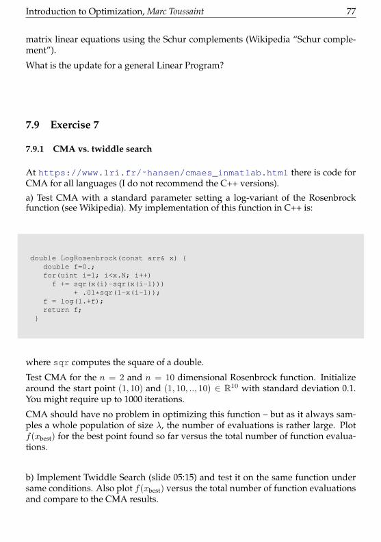
Introduction to Optimization, Marc Toussaint 77
matrix linear equations using the Schur complements (Wikipedia “Schur comple-ment”).
What is the update for a general Linear Program?
7.9 Exercise 7
7.9.1 CMA vs. twiddle search
At https://www.lri.fr/˜hansen/cmaes_inmatlab.html there is code forCMA for all languages (I do not recommend the C++ versions).
a) Test CMA with a standard parameter setting a log-variant of the Rosenbrockfunction (see Wikipedia). My implementation of this function in C++ is:
double LogRosenbrock(const arr& x) {double f=0.;for(uint i=1; i<x.N; i++)f += sqr(x(i)-sqr(x(i-1)))
+ .01*sqr(1-x(i-1));f = log(1.+f);return f;
}
where sqr computes the square of a double.
Test CMA for the n = 2 and n = 10 dimensional Rosenbrock function. Initializearound the start point (1, 10) and (1, 10, .., 10) ∈ R10 with standard deviation 0.1.You might require up to 1000 iterations.
CMA should have no problem in optimizing this function – but as it always sam-ples a whole population of size λ, the number of evaluations is rather large. Plotf(xbest) for the best point found so far versus the total number of function evalua-tions.
b) Implement Twiddle Search (slide 05:15) and test it on the same function undersame conditions. Also plot f(xbest) versus the total number of function evaluationsand compare to the CMA results.

78 Introduction to Optimization, Marc Toussaint
7.10 Exercise 8
7.10.1 More on LP formulation
A few more exercises on standard techniques to convert problems into linear pro-grams:
Solve Exercise 4.11 (pdf page 207) from Boyd & Vandenberghe, Convex Optimization.
7.10.2 Grocery Shopping
You’re at the market and you find n offers, each represented by a set of items Aiand the respective price ci. Your goal is to buy at least one of each item for as littleas possible.
Formulate as an ILP and then define a relaxation. If possible, come up with aninterpretation for the relaxed problem.
7.10.3 Facility Location
There are n facilities with which to satisfy the needs of m clients. The cost foropening facility j is fj , and the cost for servicing client i through facility j is cij . Youhave to find an optimal way to open facilities and to associate clients to facilities.
Formulate as an ILP and then define a relaxation. If possible, come up with aninterpretation for the relaxed problem.
7.10.4 Taxicab Driver (optional)
You’re a taxicab driver in hyper-space (Rd) and have to service n clients. Each clienti has an known initial position ci ∈ Rd and a destination di ∈ Rd. You start out atposition p0 ∈ Rd and have to service all the clients while minimizing fuel use, whichis proportional to covered distance. Hyper-space is funny, so the geometry is notEuclidean and distances are Manhattan distances.
Formulate as an ILP and then define a relaxation. If possible, come up with aninterpretation for the relaxed problem.
7.10.5 Programming
Use the primal-dual interior point Newton method you programmed in the previ-ous exercises to solve the relaxed facility location for n facilities and m clients (nand m small enough that you can find the solution by hand, so about n ∈ {3, ..., 5}and m ∈ {5, 10}.

Introduction to Optimization, Marc Toussaint 79
Sample the positions of facilities and clients uniformly in [−10, 10]2. Also samplethe cost of opening a facility randomly in [1, 10]. Set the cost for servicing client iwith facility j as the euclidean distance between the two. (important: keep track ofwhat seed you are using for your RNG).
Compare the solution you found by hand to the relaxed solution, and to the re-laxed solution after rounding it to the nearest integral solution. Try to find a seedfor which the rounded solution is relatively good, and one for which the roundedsolution is pretty bad.
7.11 Exercise 8
7.11.1 Global Optimization
Find an implementation of Gaussian Processes for your language of choice (e.g.python: scikit-learn, or Sheffield/Gpy; octave/matlab: gpml). and implementUCB. Test your implementation with different hyperparameters (Find the best com-bination of kernel and its parameters in the GP) on the following 2D global opti-mization problems:
• the 2d Rosenbrock function.
• the Rastrigin function as defined in exercise e03 with a = 6.
7.11.2 Constrained Global Bayes Optimization?
On slide 5:18 it is speculated that one could consider a constrained blackbox opti-mization problem as well. How could one approach this in the UCB manner?
7.12 Exercise 10
7.12.1 BlackBox Local Search Programming
1a) Implement Greedy Local Search and Stochastic Local Search
1b) Implement Random Restarts
1c) Implement Iterated Local Search
Use the above methods on the Rosenbrock and the Rastrigin functions.

80 Introduction to Optimization, Marc Toussaint
7.12.2 Neighborhoods
2a) Define a deterministic and a stochastic notion of neighborhood which is appro-priate for the Grocery Shopping problem defined in e08.
2b) Define a deterministic and a stochastic notion of neighborhood which is appro-priate for the Facility Location problem defined in e08.
2c) Define a deterministic and a stochastic notion of neighborhood which is appro-priate for the Taxicab problem defined in e08.
7.13 Exercise 10
7.13.1 BlackBox Local Search Programming
1a) Implement Greedy Local Search and Stochastic Local Search
1b) Implement Random Restarts
1c) Implement Iterated Local Search
Use the above methods on the Rosenbrock and the Rastrigin functions.
7.13.2 Neighborhoods
2a) Define a deterministic and a stochastic notion of neighborhood which is appro-priate for the Grocery Shopping problem defined in e08.
2b) Define a deterministic and a stochastic notion of neighborhood which is appro-priate for the Facility Location problem defined in e08.
2c) Define a deterministic and a stochastic notion of neighborhood which is appro-priate for the Taxicab problem defined in e08.
7.14 Exercise 11
7.14.1 Model Based Optimization
1) Implement Model-based optimization as described in slide 06:33 and use it tosolve the usual Raistringen and Rosenbrock functions.
Visualize the current estimated model at each step of the optimization procedure.
Hints:
• Try out both a quadratic model φ2(x) = [1, x1, x2, x21, x
22, x1x2] and a linear
one φ1(x) = [1, x1, x2].

Introduction to Optimization, Marc Toussaint 81
• Initialize the model sampling .5(n+ 1)(n+ 2) (in the case of quadratic model)or n+ 1 (in the case of linear model) points around the starting position.
• For any given set of datapoints D, compute β = (X>X)−1X>y, where X con-tains (row-wise) the data points (either φ1 or φ2) inD, and y are the respectivefunction evaluations.
• Compute det(D) as det(X>X).
• Solve the local maximization problem in line 12 directly by inspecting a finitenumber of points in a grid-like structure around the current point.
• The ∆ in line 18 should just be the current dataset D.
• Always maintain at least .5(n + 1)(n + 2) (quadratic) or n + 1 (linear) data-points in D. This almost-surely ensures that the regression parameter β is welldefined.
7.14.2 No Free Lunch Theorems
Broadly speaking, the No Free Lunch Theorems state that an algorithm can be saidto outperform another one only if certain assumptions are made about the problemwhich is being solved itself. In other words, algorithms perform in average exactlythe same, if no restriction or assumption is made on the type of problem itself.Algorithms outperform each other only w.r.t specific classes of problems.
2a) Read the publication “No Free Lunch Theorems for Optimization” by Wolpertand Macready and get a better feel for what the statements are about.
2b, 2c, 2d) You are given an optimization problem where the search space is a setX with size 100, and the cost space Y is the set of integers {1, . . . , 100}. Come upwith three different algorithms, and three different assumptions about the problem-space such that each algorithm outperforms the others in one of the assumptions.
Try to be creative, or you will all come up with the same “obvious” answers.
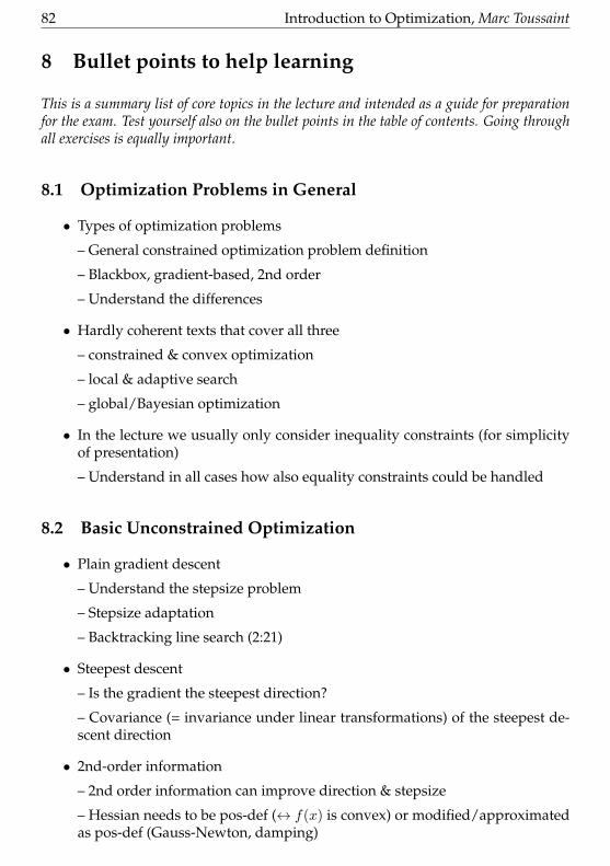
82 Introduction to Optimization, Marc Toussaint
8 Bullet points to help learning
This is a summary list of core topics in the lecture and intended as a guide for preparationfor the exam. Test yourself also on the bullet points in the table of contents. Going throughall exercises is equally important.
8.1 Optimization Problems in General
• Types of optimization problems
– General constrained optimization problem definition
– Blackbox, gradient-based, 2nd order
– Understand the differences
• Hardly coherent texts that cover all three
– constrained & convex optimization
– local & adaptive search
– global/Bayesian optimization
• In the lecture we usually only consider inequality constraints (for simplicityof presentation)
– Understand in all cases how also equality constraints could be handled
8.2 Basic Unconstrained Optimization
• Plain gradient descent
– Understand the stepsize problem
– Stepsize adaptation
– Backtracking line search (2:21)
• Steepest descent
– Is the gradient the steepest direction?
– Covariance (= invariance under linear transformations) of the steepest de-scent direction
• 2nd-order information
– 2nd order information can improve direction & stepsize
– Hessian needs to be pos-def (↔ f(x) is convex) or modified/approximatedas pos-def (Gauss-Newton, damping)

Introduction to Optimization, Marc Toussaint 83
• Newton method
– Definition
– Adaptive stepsize & damping
• Gauss-Newton
– f(x) is a sum of squared cost terms
– The approx. Hessian 2∇φ(x)>∇φ(x) is always semi-pos-def!
• Quasi-Newton
– Accumulate gradient information to approximate a Hessian
– BFGS, understand the term δδ>
δ>y
• Conjugate gradient
– New direction d′ should be “orthogonal” to the previous d, but relative tothe local quadratic shape, d′>Ad = 0 (= d′ and d are conjugate)
– On quadratic functions CG converges in n iterations
• Rprop
– Seems awfully hacky
– Every coordinate is treated separately. No invariance under rotations/transformations.
– Change in gradient sign→ reduce stepsize; else increase
– Works surprisingly well and robust in practice
• Convergence
– With perfect line search, the extrem (finite & positive!) eigenvalues of theHessian ensure convergence
– The Wolfe conditions (acceptance criterion for backtracking line search) en-sure a “significant” decrease in f(x), which also leads to convergence
• Trust region
– Alternative to stepsize adaptation and backtracking
• Evaluating optimization costs
– Be aware in differences in convention. Sometimes “1 iteration”=many func-tion evaluations (line search)
– Best: always report on # function evaluations

84 Introduction to Optimization, Marc Toussaint
8.3 Constrained Optimization
• Overview
– General problem definition
– Convert to series of unconstrained problems: penalty, log barrier, & Aug-mented Lagrangian methods
– Convert to series of QPs and line search: Sequential Quadratic Program-ming
– Convert to larger unconstrained problem: primal-dual Newton method
– Convert to other constrained problem: dual problem
• Log barrier method
– Definition
– Understand how the barrier gets steeper with µ→ 0 (not µ→∞!)
– Iterativly decreasing µ generates the central path
– The gradient of the log barrier generates a Lagrange term with λi = − µgi(x) !
→ Each iteration solves the modified (approximate) KKT condition
• Squared penalty method
– Definition
– Motivates the Augmented Lagrangian
• Augmented Lagrangian
– Definition
– Role of the squared penalty: “measure” how strong f pushes into the con-straint
– Role of the Lagrangian term: generate counter force
– Unstand that the λ update generates the “desired gradient”
• The Lagrangian
– Definition
– Using the Lagrangian to solve constrained problems on paper (set both,∇xL(x, λ) = 0 and ∇λL(x, λ) = 0)
– “Balance of gradients” and the first KKT condition
– Understand in detail the full KKT conditions
– Optima are necessarily saddle points of the Lagrangian
– minx L↔ first KKT↔ balance of gradients
– maxλ L↔ complementarity KKT↔ constraints
Introduction to Optimization, Marc Toussaint 85
• Lagrange dual problem
– primal problem: minx maxl≥0 L(x, λ)
– dual problem: maxλ≥0 minx L(x, λ)
– Definition of Lagrange dual
– Lower bound and strong duality
• Primal-dual Newton method to solve KKT conditions
– Definition & description
• Phase I optimization
– Nice trick to find feasible initialization
8.4 Convex Optimization
• Definitions
– Convex, quasi-convex, uni-modal functions
– Convex optimization problem
• Linear Programming
– General and standard form definition
– Converting into standard form
– LPs are efficiently solved using 2nd-order log barrier, augmented Lagrangianor primal-dual methods
– Simplex Algorithm is classical alternative; walks on the constraint edgesinstead of the interior
• Application of LP:
– Very important application of LPs: LP-relaxations of integer linear programs
• Quadratic Programming
– Definition
– QPs are efficiently solved using 2nd-order log barrier, augmented Lagrangianor dual-primal methods
– Sequential QP solves general (non-quadratic) problems by defining a localQP for the step direction followed by a line search in that direction
86 Introduction to Optimization, Marc Toussaint
8.5 Search methods for Blackbox optimization
• Overview
– Basic downhill running: mostly ignore the collected data
– Use the data to shape search: stochastic search, EAs, model-based search
– Bayesian (global) optimization
• Basic downhill running
– Greedy local search: defined by neighborhood N
– Stochastic local search: defined by transition probability q(y|x)
– Simulated Annealing: also accepts “bad” steps depending on temperature;theoretically highly relevant, practically less
– Random restarts of local search can be efficient
– Iterated local search: use meta-neighborhood N∗ to restart
– Coordinate & Pattern search, Twiddle: use heuristics to walk along coordi-nates
– Nelder-Mead simplex method: reflect, expand, contract, shrink
• Stochastic Search
– General scheme: sample from pθ(x), update θ
– Understand the crucial role of θ: θ captures all that is maintained and up-dated depending on the data; in EAs, θ is a population; in ESs, θ are parame-ters of a Gaussian
– Categories of EAs: ES, GA, GP, EDA
– CMA: adapting C and σ based on the path of the mean
• Model-based Optimization
– Precursor of Bayesian Optimization
– Core: smart ways to keep data D healthy
8.6 Bayesian Optimization
• Multi-armed bandit framework
– Problem definition
– Understand the concepts of exploration, exploitation & belief
– Optimal Optimization would imply to plan (exactly) through belief space
– Upper Confidence Bound (UCB) and confidence interval
– UCB is optimistic

Introduction to Optimization, Marc Toussaint 87
• Global optimization
– Global optimization = infinite bandits
– Locally correlated bandits→ Gaussian Process beliefs
– Maximum Probability of Improvement
– Expected Improvement
– GP-UCB
• Potential pitfalls
– Choice of prior belief (e.g. kernel of the GP) is crucial
– Pure variance-based sampling for radially symmetric kernel ≈ grid sam-pling

IndexAugmented Lagrangian method (3:14),
Backtracking (2:5),Bandits (5:4),Belief planning (5:8),Blackbox optimization: definition (6:1),
Blackbox optimization: overview (6:3),
Broyden-Fletcher-Goldfarb-Shanno (BFGS)(2:25),
Central path (3:9),Conjugate gradient (2:28),Constrained optimization (3:1),Coordinate search (6:14),Covariance Matrix Adaptation (CMA)
(6:24),Covariant gradient descent (2:13),
Estimation of Distribution Algorithms(EDAs) (6:28),
Evolutionary algorithms (6:23),Expected Improvement (5:24),Exploration, Exploitation (5:6),
Function types: covex, quasi-convex,uni-modal (4:1),
Gauss-Newton method (2:20),Gaussian Processes as belief (5:19),General stochastic search (6:20),Global Optimization as infinite bandits
(5:17),GP-UCB (5:24),Gradient descent convergence (2:8),Greedy local search (6:5),
Implicit filtering (6:34),Iterated local search (6:11),
Karush-Kuhn-Tucker (KKT) conditions(3:25),
Lagrange dual problem (3:29),Lagrangian: definition (3:21),Lagrangian: relation to KKT (3:24),Lagrangian: saddle point view (3:27),
Line search (2:5),Linear program (LP) (4:6),Log barrier as approximate KKT (3:33),
Log barrier method (3:6),LP in standard form (4:7),LP-relaxations of integer programs (4:15),
Maximal Probability of Improvement(5:24),
Model-based optimization (6:31),
Nelder-Mead simplex method (6:16),Newton direction (2:14),Newton method (2:15),
Pattern search (6:15),Phase I optimization (3:40),Plain gradient descent (2:1),Primal-dual interior-point Newton method
(3:36),
Quadratic program (QP) (4:6),Quasi-Newton methods (2:23),
Random restarts (6:10),Rprop (2:35),
Sequential quadratic programming (4:23),
Simplex method (4:11),Simulated annealing (6:7),Squared penalty method (3:12),Steepest descent direction (2:11),Stepsize adaptation (2:4),Stepsize and step direction as core is-
sues (2:2),
88

Introduction to Optimization, Marc Toussaint 89
Stochastic local search (6:6),
Trust region (3:41),Types of optimization problems (1:3),
Upper Confidence Bound (UCB) (5:12),
Variable neighborhood search (6:13),
Wolfe conditions (2:7),