Introduction to Optimization - École Polytechnique · Introduction to Optimization Approximation...

Introduction to Optimization

Approximation Algorithms and Heuristics

Dimo Brockhoff

Inria Saclay – Ile-de-France

November 21, 2016

École Centrale Paris, Châtenay-Malabry, France

2Introduction to Optimization @ ECP, Nov. 21, 2016© Dimo Brockhoff, Inria 2

Exercise:

The Knapsack Problem and Dynamic

Programming

http://chercheurs.lille.inria.fr/

~brockhof/introoptimization/exercises.php


I hope it became clear...

...what the algorithm design idea of dynamic programming is

...for which problem types is is supposed to be suitable

...and how to apply the idea to the knapsack problem

Conclusions


Date Topic

Fri, 7.10.2016 Introduction

Fri, 28.10.2016 D Introduction to Discrete Optimization + Greedy algorithms I

Fri, 4.11.2016 D Greedy algorithms II + Branch and bound

Fri, 18.11.2016 D Dynamic programming

Mon, 21.11.2016

in S103-S105

D Approximation algorithms and heuristics

Fri, 25.11.2016

in S103-S105

C Introduction to Continuous Optimization I

Mon, 28.11.2016 C Introduction to Continuous Optimization II

Mon, 5.12.2016 C Gradient-based Algorithms

Fri, 9.12.2016 C Stochastic Optimization and Derivative Free Optimization I

Mon, 12.12.2016 C Stochastic Optimization and Derivative Free Optimization II

Fri, 16.12.2016 C Benchmarking Optimizers with the COCO platform

Wed, 4.1.2017 Exam

Course Overview

all classes last 3h15 and take place in S115-S117 (see exceptions)


Approximation Algorithms

a greedy approximation algorithm for bin packing

an FPTAS for the KP

Overview of (Randomized) Search Heuristics

randomized local search

variable neighborhood search

tabu search

evolutionary algorithms

[exercise: simple randomized algorithms for the knapsack

problem]

Potential Master's/PhD thesis projects

Overview of Today’s Lecture


Exact

brute-force often too slow

better strategies such as dynamic programming & branch

and bound

still: often exponential runtime


guarantee of low run time

guarantee of high quality solution

obstacle: difficult to prove these guarantees

Heuristics

intuitive algorithms

guarantee to run in short time

often no guarantees on solution quality

Coping with Difficult Problems

(now)

(later today)


An algorithm is a ρ-approximation algorithm for problem Π if, for

each problem instance of Π, it outputs a feasible solution which

function value is within a ratio ρ of the true optimum for that

instance.

An algorithm A is an approximation scheme for a minimization*

problem Π if for any instance I of Π and a parameter ε>0, it outputs

a solution s with f Π(I,s) ≤ (1+ε) ∙ OPT .

An approximation scheme is called polynomial time approximation

scheme (PTAS) if for a fixed ε>0, its running time is polynomially

bounded in the size of the instance I.

note: runtime might be exponential in 1/ε actually!

An approximation scheme is a fully polynomial time approximation

scheme (FPTAS) if its runtime is bounded polynomially in both the

size of the input I and in 1/ε.

Approximations, PTAS, and FPTAS


only example algorithm(s)

no detailed proofs here due to the time restrictions of the class

rather spend more time on the heuristics part and the exercise

Actually Two Examples:

a greedy approximation algorithm for bin packing

an FPTAS for the KP

Today’s Lecture


Bin Packing Problem

Given a set of n items with sizes a1, a2, ..., an. Find an

assignment of the ai’s to bins of size V such that the number of

bins is minimal and the sum of the sizes of all items assigned to

each bin is ≤ V.

Known Facts

no optimization algorithm reaches a better than 3/2

approximation in polynomial time (not shown here)

greedy first-fit approach already yields an approximation

algorithm with ρ-ratio of 2

Bin Packing (BP)


First-Fit Algorithm

without sorting the items do:

put each item into the first bin where it fits

if it does not fit anywhere, open a new bin

Theorem: First-Fit algorithm is a 2-approximation algorithm

Proof: Assume First Fit uses m bins. Then, at least m-1 bins are more

than half full (otherwise, move items).

because m and OPT are integer

First-Fit Approach

0.5 0.8 0.20.40.3 0.2 0.2

0.5 0.3 0.4

0.8

0.2 0.2 0.2


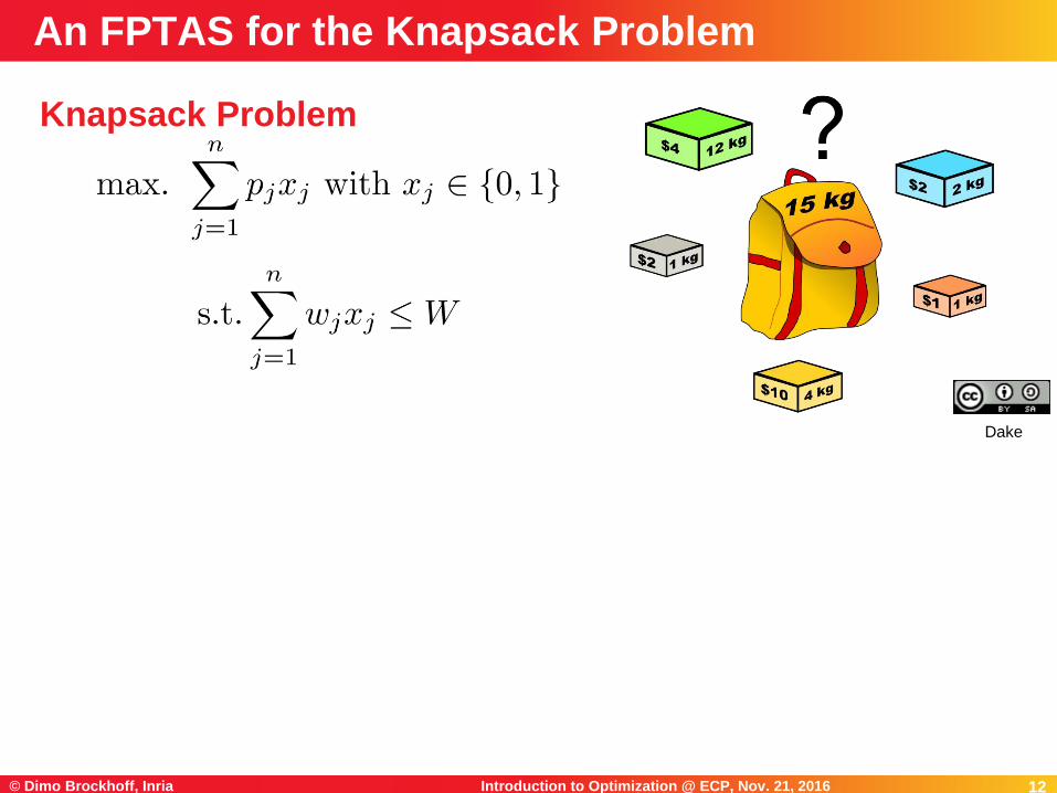
Knapsack Problem

An FPTAS for the Knapsack Problem

Dake


Similar to this week’s exercise, we can design a dynamic

programming algorithm for which

a subproblem is restricting the items to {1, ..., k} and

searches for the lightest packing with prefixed profit P

runs in O(n2Pmax)

What strange runtime is O(n2Pmax)?

Answer: pseudo-polynomial (polynomial if Pmax would be

polynomial in input size)

Idea behind FPTAS:

scale the profits smartly to to make Pmax

polynomially bounded

prove that dynamic programming approach computes profit

of at least (1-ε)∙OPT (not shown here)

An FPTAS for the Knapsack Problem

maxP

npi


(Randomized) Search Heuristics


often, problem complicated and not much time available to

develop a problem-specific algorithm

search heuristics are a good choice:

relatively easy to implement

easy to adapt/change/improve

e.g. when the problem formulation changes in an early

product design phase

or when slightly different problems need to be solved

over time

Motivation General Search Heuristics


Randomized Local Search (RLS)

Variable Neighborhood Search (VNS)

Tabu Search (TS)

Evolutionary Algorithms (EAs)

Lecture Overview


For most (stochastic) search heuristics in discrete domain, we need

to define a neighborhood structure

which search points are close to each other?

Example: k-bit flip / Hamming distance k neighborhood

search space: bitstrings of length n (Ω={0,1}n)

two search points are neighbors if their Hamming

distance is k

in other words: x and y are neighbors if we can flip

exactly k bits in x to obtain y

0001001101 is neighbor of

0001000101 for k=1

0101000101 for k=2

1101000101 for k=3

Neighborhoods


Idea behind (Randomized) Local Search:

explore the local neighborhood of the current solution (randomly)

Pure Random Search:

go to randomly chosen neighbor (not dependent on obj. function)

First Improvement Local Search, Randomized Local Search (RLS):

go to first (randomly) chosen neighbor which is better

Best Improvement Strategy:

always go to the best neighbor

not random anymore

computationally expensive if neighborhood large

Randomized Local Search (RLS)


Main Idea: [Mladenovic and P. Hansen, 1997]

change the neighborhood from time to time

local optima are not the same for different neighborhood

operators

but often close to each other

global optimum is local optimum for all neighborhoods

rather a framework than a concrete algorithm

e.g. deterministic and stochastic neighborhood changes

typically combined with (i) first improvement, (ii) a random

order in which the neighbors are visited and (iii) restarts

N. Mladenovic and P. Hansen (1997). "Variable neighborhood search". Computers

and Operations Research 24 (11): 1097–1100.

Variable Neighborhood Search


Disadvantages of local searches (with or without varying

neighborhoods)

they get stuck in local optima

have problems to traverse large plateaus of equal objective

function value (“random walk”)

Tabu search addresses these by

allowing worsening moves if all neighbors are explored

introducing a tabu list of temporarily not allowed moves

those restricted moves are

problem-specific and

can be specific solutions or not permitted “search

directions” such as “don’t include this edge anymore” or

“do not flip this specific bit”

the tabu list is typically restricted in size and after a while,

restricted moves are permitted again

Tabu Search


One class of (bio-inspired) stochastic optimization algorithms:

Evolutionary Algorithms (EAs)

Class of optimization algorithms

originally inspired by the idea of

biological evolution

selection, mutation, recombination

Stochastic Optimization Algorithms

1859


Classical Optimization Evolutionary Computation

variables or parameters variables or chromosomes

candidate solution

vector of decision variables /

design variables / object

variables

individual, offspring, parent

set of candidate solutions population

objective function

loss function

cost function

error function

fitness function

iteration generation

Metaphors


Generic Framework of an EA

Important:

representation (search space)

initialization

evaluation

evaluation

potential

parents

offspring

parents

crossover/

mutation

mating

selection

environmental

selection

stop?

best individual

stochastic operators

“Darwinism”

stopping criteria


Genetic Algorithms (GA)

J. Holland 1975 and D. Goldberg (USA)

Evolution Strategies (ES)

I. Rechenberg and H.P. Schwefel, 1965 (Berlin)

Evolutionary Programming (EP)

L.J. Fogel 1966 (USA)

Genetic Programming (GP)

J. Koza 1990 (USA)

nowadays one umbrella term: evolutionary algorithms

The Historic Roots of EAs


The genotype – phenotype mapping

related to the question: how to come up with a fitness of

each individual from the representation?

related to DNA vs. actual animal (which then has a fitness)

Fitness of an individual not always = f(x)

include constraints

include diversity

others

but needed: always a total order on the solutions

Genotype – Phenotype mapping


Several possible ways to handle constraints, e.g.:

resampling until a new feasible point is found (“often bad idea”)

penalty function approach: add constraint violation term

(potentially scaled, see also the Lagrangian in the continuous

part of the lecture)

repair approach: after generation of a new point, repair it (e.g.

with a heuristic) to become feasible again if infeasible

continue to use repaired solution in the population or

use repaired solution only for the evaluation?

multiobjective approach: keep objective function and constraint

functions separate and try to optimize all of them in parallel

some more...

Handling Constraints


Examples for some EA parts(for discrete search spaces)


Selection is the major determinant for specifying the trade-off

between exploitation and exploration

Selection is either

stochastic or deterministic

e.g. fitness proportional

e.g. via a tournament

Mating selection (selection for variation): usually stochastic

Environmental selection (selection for survival): often deterministic

Selection

Disadvantage:

depends on

scaling of f

e.g. (µ+λ), (µ,λ)

best µ from

offspring and

parents

best µ from

offspring only


Variation aims at generating new individuals on the basis of those

individuals selected for mating

Variation = Mutation and Recombination/Crossover

mutation: mut:

recombination: recomb: where and

choice always depends on the problem and the chosen

representation

however, there are some operators that are applicable to a wide

range of problems and tailored to standard representations such

as vectors, permutations, trees, etc.

Variation Operators


Two desirable properties for mutation operators:

“exhaustiveness”: every solution can be generated from every

other with a probability greater than 0

“locality”:

Desirable property of recombination operators (“in-between-ness”):

Variation Operators: Guidelines


Swap:

Scramble:

Invert:

Insert:

Examples of Mutation Operators on Permutations


1-point crossover

n-point crossover

uniform crossover

Examples of Recombination Operators: {0,1}n

choose each bit

independently from

one parent or another


search space of all binary strings of length 𝑛, maximization

uniform initialization

generational cycle of the population:

evaluation of solutions

mating selection (e.g. roulette wheel)

crossover (e.g. 1-point)

environmental selection (e.g. plus-selection)

A Canonical Genetic Algorithm


EAs are generic algorithms (randomized search heuristics,

meta-heuristics, ...) for black box optimization

no or almost no assumptions on the objective function

They are typically less efficient than problem-specific

(exact) algorithms (in terms of #funevals)

not the case in the continuous case (we will see later)

Allow for an easy and rapid implementation and therefore

to find good solutions fast

easy to incorporate problem-specific knowledge to improve

the algorithm

Conclusions


Potential Master's/PhD thesis

projects


http://randopt.gforge.inria.fr/thesisprojects/

Potential Research Topics for Master's/PhD Theses


More projects without the involvement of companies:

stopping criteria in multiobjective optimization

large-scale variants of CMA-ES

algorithms for expensive optimization based on CMA-ES

all above: relatively flexible between theoretical and practical projects

Coco-related:

implementing and benchmarking algorithms for expensive opt.

data mining performance results

Potential Research Topics for Master's/PhD Theses


I hope it became clear...

...that approximation algorithms are often what we can hope for

in practice (might be difficult to achieve guarantees though)

...that heuristics is what we typically can afford in practice (no

guarantees and no proofs)

Conclusions

Introduction to Optimization - École Polytechnique · Introduction to Optimization Approximation...

Documents

Transcript of Introduction to Optimization - École Polytechnique · Introduction to Optimization Approximation...