Introduction to OpenACC - Boston UniversityGPU is an accelerator •GPU is a device on a CPU-based...
46
Introduction to OpenACC Shaohao Chen Research Computing Services Information Services and Technology Boston University
Transcript of Introduction to OpenACC - Boston UniversityGPU is an accelerator •GPU is a device on a CPU-based...

Introduction to OpenACC
Shaohao Chen
Research Computing Services
Information Services and Technology
Boston University

Outline
• Introduction to GPU and OpenACC
• Basic syntax and the first OpenACC program: SAXPY
• Kernels vs. parallel directives
• An example: Laplace solver in OpenACC
The first try
Data transfer between GPU and CPU/host
Data race and the reduction clause
• GPU and OpenACC task granularities
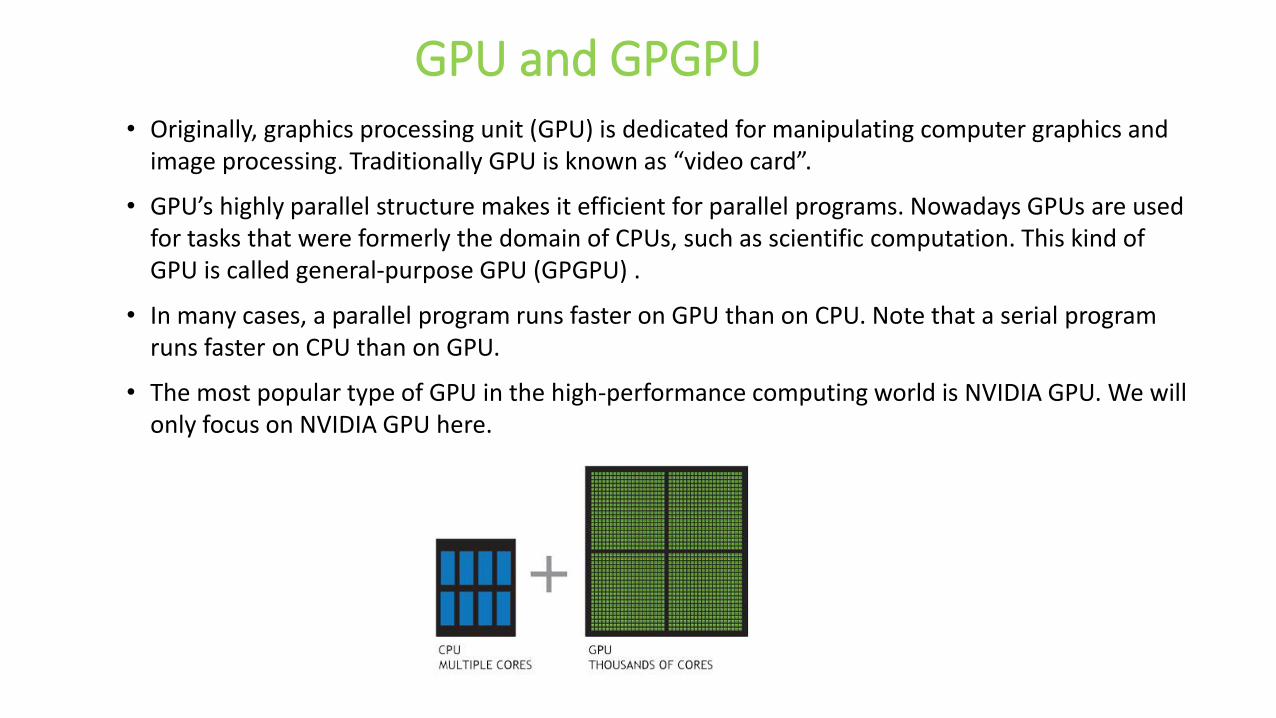
GPU and GPGPU• Originally, graphics processing unit (GPU) is dedicated for manipulating computer graphics and
image processing. Traditionally GPU is known as “video card”.
• GPU’s highly parallel structure makes it efficient for parallel programs. Nowadays GPUs are used for tasks that were formerly the domain of CPUs, such as scientific computation. This kind of GPU is called general-purpose GPU (GPGPU) .
• In many cases, a parallel program runs faster on GPU than on CPU. Note that a serial program runs faster on CPU than on GPU.
• The most popular type of GPU in the high-performance computing world is NVIDIA GPU. We will only focus on NVIDIA GPU here.

GPU is an accelerator
• GPU is a device on a CPU-based system. GPU is connected to CPU through PCI bus.
• Computer program can be parallelized and accelerated on GPU.
• CPU and GPU has separated memories. Data transfer between CPU and GPU is required for programming.

Three ways to accelerate applications on GPU
What is OpenACC
• OpenACC (for Open Accelerators) is a programming standard for parallel computing on accelerators (mostly on NIVDIA GPU).
• It is designed to simplify GPU programming.
• The basic approach is to insert special comments (directives) into the code so as to offload computation onto GPUs and parallelize the code at the level of GPU (CUDA) cores.
• It is possible for programmers to create an efficient parallel OpenACC code with only minor modifications to a serial CPU code.
What are compiler directives?
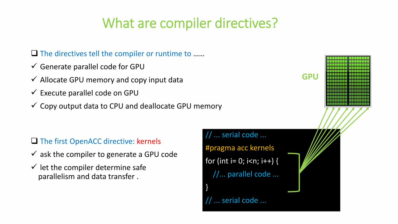
The directives tell the compiler or runtime to ……
Generate parallel code for GPU
Allocate GPU memory and copy input data
Execute parallel code on GPU
Copy output data to CPU and deallocate GPU memory
// ... serial code ...
#pragma acc kernels
for (int i= 0; i<n; i++) {
//... parallel code ...
}
// ... serial code ...
The first OpenACC directive: kernels
ask the compiler to generate a GPU code
let the compiler determine safe parallelism and data transfer .
GPU

OpenACC Directive syntax
• C
#pragma acc directive [clause [,] clause] …]…
often followed by a structured code block
• Fortran
!$acc directive [clause [,] clause] …]...
often paired with a matching end directive surrounding a structured code block
!$acc end directive

The first OpenACC program: SAXPY
Example: Compute a*x + y, where x and y are vectors, and a is a scalar.
int main(int argc, char **argv){
int N=1000;
float a = 3.0f;
float x[N], y[N];
for (int i = 0; i < N; ++i) {
x[i] = 2.0f;
y[i] = 1.0f;
}
#pragma acc kernels
for (int i = 0; i < N; ++i) {
y[i] = a * x[i] + y[i];
}
}
program main
integer :: n=1000, i
real :: a=3.0
real, allocatable :: x(:), y(:)
allocate(x(n),y(n))
x(1:n)=2.0
y(1:n)=1.0
!$acc kernels
do i=1,n
y(i) = a * x(i) + y(i)
enddo
!$acc end kernels
end program main
C Fortran
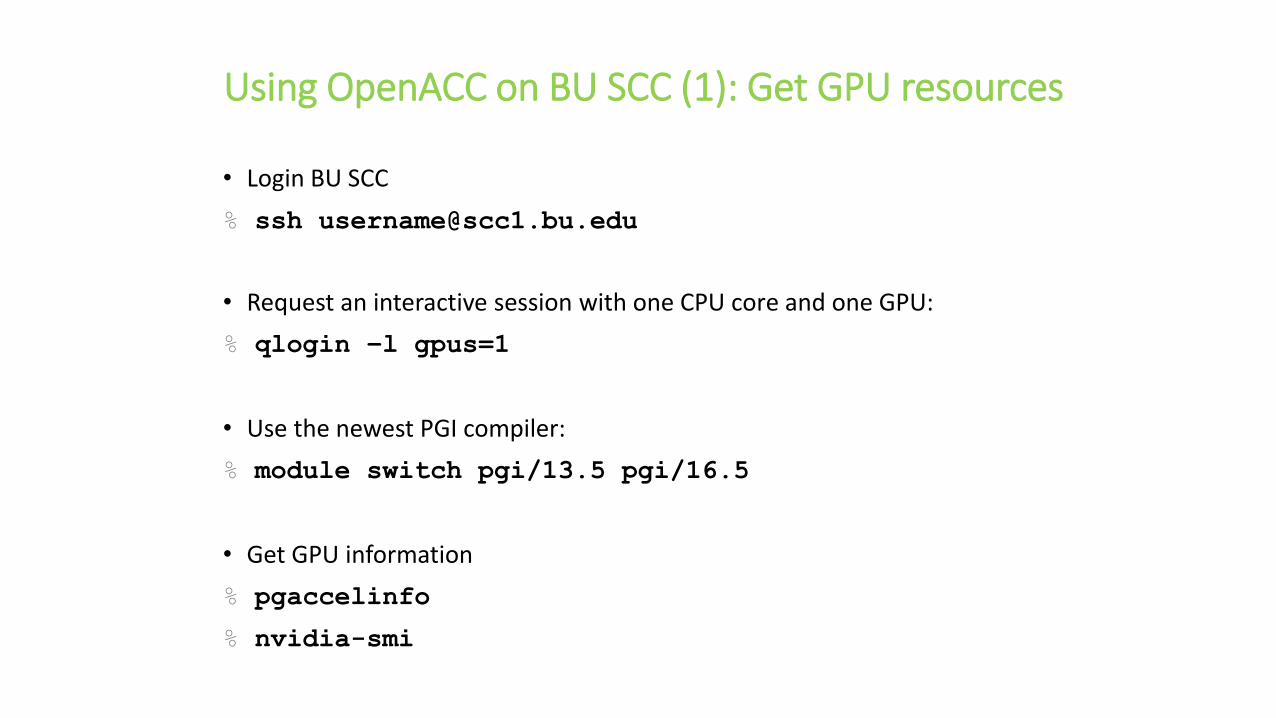
Using OpenACC on BU SCC (1): Get GPU resources
• Login BU SCC
% ssh [email protected]
• Request an interactive session with one CPU core and one GPU:
% qlogin –l gpus=1
• Use the newest PGI compiler:
% module switch pgi/13.5 pgi/16.5
• Get GPU information
% pgaccelinfo
% nvidia-smi
Using OpenACC on BU SCC (2): Compile and Run
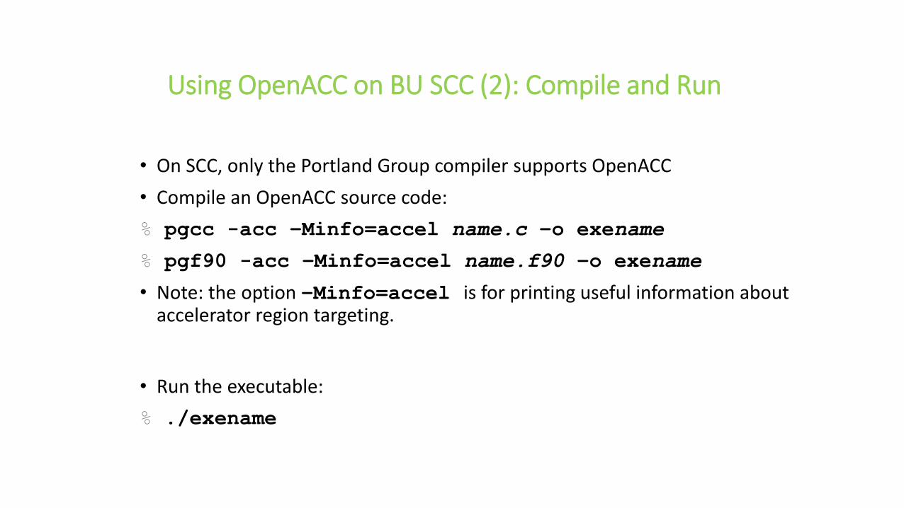
• On SCC, only the Portland Group compiler supports OpenACC
• Compile an OpenACC source code:
% pgcc -acc –Minfo=accel name.c –o exename
% pgf90 -acc –Minfo=accel name.f90 –o exename
• Note: the option –Minfo=accel is for printing useful information about accelerator region targeting.
• Run the executable:
% ./exename

1) Login BU SCC and get an interactive session with GPU resources.
2) Provided a serial SAXPY code in C or Fortran, parallelize it using OpenACCdirectives.
3) Compile and run the SAXPY code.
Exercise 1: SAXPY
Analysis of the compiling output
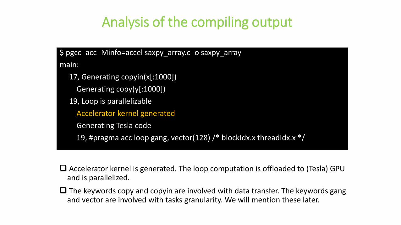
Accelerator kernel is generated. The loop computation is offloaded to (Tesla) GPU and is parallelized.
The keywords copy and copyin are involved with data transfer. The keywords gang and vector are involved with tasks granularity. We will mention these later.
$ pgcc -acc -Minfo=accel saxpy_array.c -o saxpy_array
main:
17, Generating copyin(x[:1000])
Generating copy(y[:1000])
19, Loop is parallelizable
Accelerator kernel generated
Generating Tesla code
19, #pragma acc loop gang, vector(128) /* blockIdx.x threadIdx.x */
Data dependency
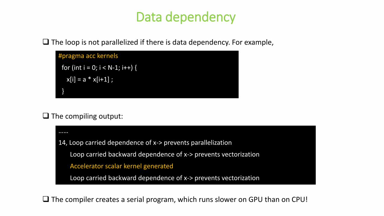
The loop is not parallelized if there is data dependency. For example,
#pragma acc kernels
for (int i = 0; i < N-1; i++) {
x[i] = a * x[i+1] ;
}
The compiling output:
……
14, Loop carried dependence of x-> prevents parallelization
Loop carried backward dependence of x-> prevents vectorization
Accelerator scalar kernel generated
Loop carried backward dependence of x-> prevents vectorization
The compiler creates a serial program, which runs slower on GPU than on CPU!
Pointer aliasing in C (1)
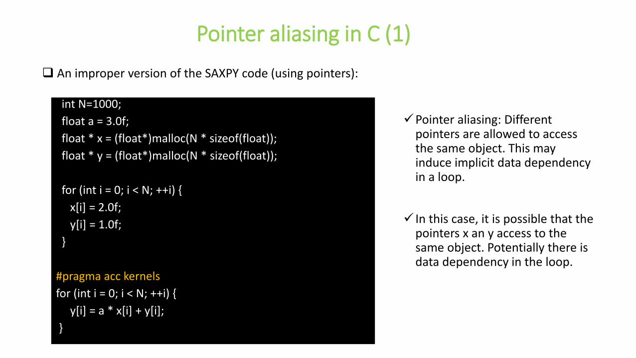
An improper version of the SAXPY code (using pointers):
int N=1000;
float a = 3.0f;
float * x = (float*)malloc(N * sizeof(float));
float * y = (float*)malloc(N * sizeof(float));
for (int i = 0; i < N; ++i) {
x[i] = 2.0f;
y[i] = 1.0f;
}
#pragma acc kernels
for (int i = 0; i < N; ++i) {
y[i] = a * x[i] + y[i];
}
Pointer aliasing: Different pointers are allowed to access the same object. This may induce implicit data dependency in a loop.
In this case, it is possible that the pointers x an y access to the same object. Potentially there is data dependency in the loop.
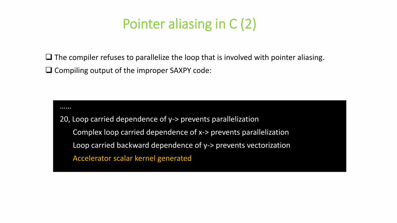
The compiler refuses to parallelize the loop that is involved with pointer aliasing.
Compiling output of the improper SAXPY code:
……
20, Loop carried dependence of y-> prevents parallelization
Complex loop carried dependence of x-> prevents parallelization
Loop carried backward dependence of y-> prevents vectorization
Accelerator scalar kernel generated
Pointer aliasing in C (2)
Use restrict to avoid pointer aliasing
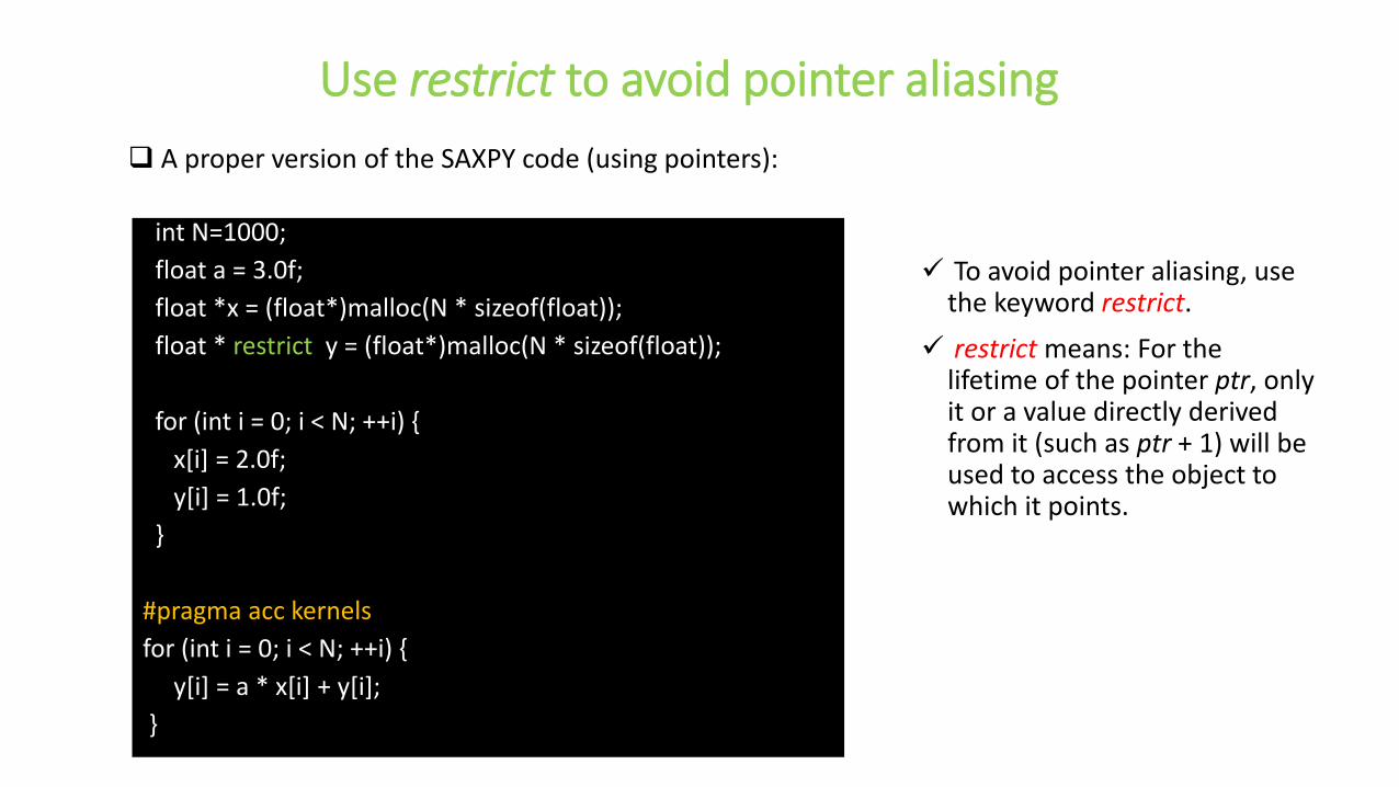
A proper version of the SAXPY code (using pointers):
int N=1000;
float a = 3.0f;
float *x = (float*)malloc(N * sizeof(float));
float * restrict y = (float*)malloc(N * sizeof(float));
for (int i = 0; i < N; ++i) {
x[i] = 2.0f;
y[i] = 1.0f;
}
#pragma acc kernels
for (int i = 0; i < N; ++i) {
y[i] = a * x[i] + y[i];
}
To avoid pointer aliasing, use the keyword restrict.
restrict means: For the lifetime of the pointer ptr, only it or a value directly derived from it (such as ptr + 1) will be used to access the object to which it points.
Parallel directive (1)
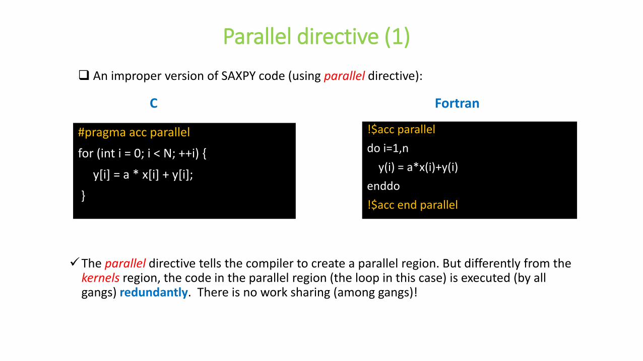
An improper version of SAXPY code (using parallel directive):
#pragma acc parallel
for (int i = 0; i < N; ++i) {
y[i] = a * x[i] + y[i];
}
The parallel directive tells the compiler to create a parallel region. But differently from the kernels region, the code in the parallel region (the loop in this case) is executed (by all gangs) redundantly. There is no work sharing (among gangs)!
!$acc parallel
do i=1,n
y(i) = a*x(i)+y(i)
enddo
!$acc end parallel
C Fortran

Parallel directive (2)
A proper version of SAXPY code (using parallel loop directive):
#pragma acc parallel loop
for (int i = 0; i < N; ++i) {
y[i] = a * x[i] + y[i];
}
It is necessary to add the keyword to loop share the works (among gangs).
In Fortran, the keyword loop can be replaced by do here.
In C, the keyword loop can be replaced by for.
!$acc parallel loop
do i=1,n
y(i) = a*x(i)+y(i)
enddo
!$acc end parallel loop
C Fortran
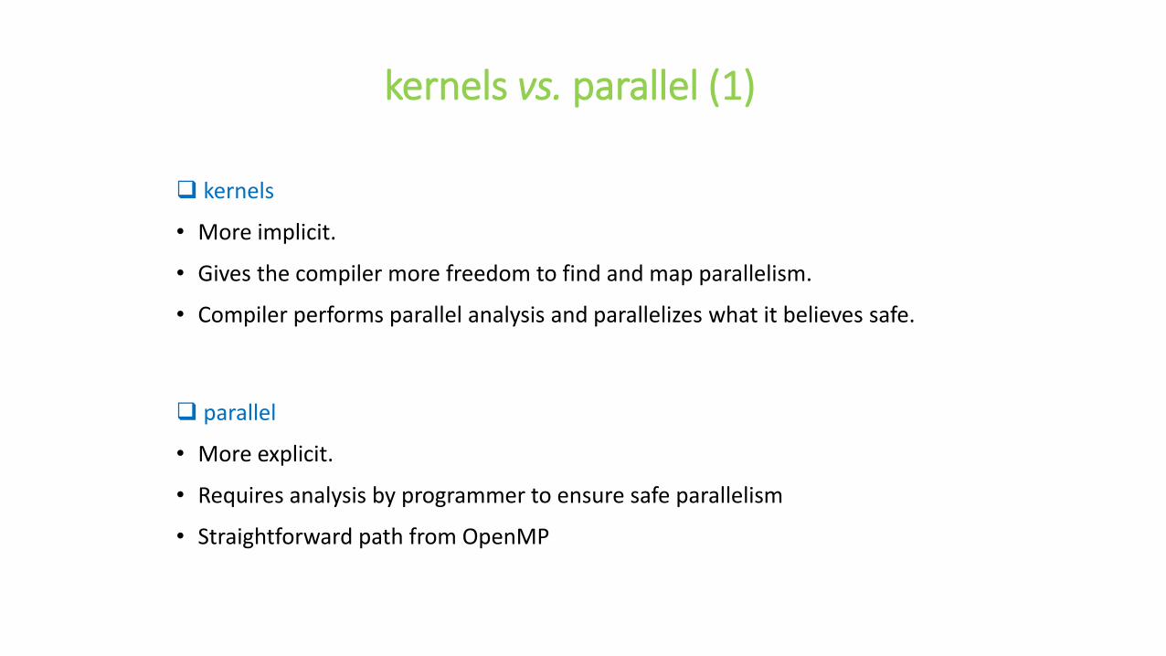
kernels vs. parallel (1)
kernels
• More implicit.
• Gives the compiler more freedom to find and map parallelism.
• Compiler performs parallel analysis and parallelizes what it believes safe.
parallel
• More explicit.
• Requires analysis by programmer to ensure safe parallelism
• Straightforward path from OpenMP
kernels vs. parallel (2)
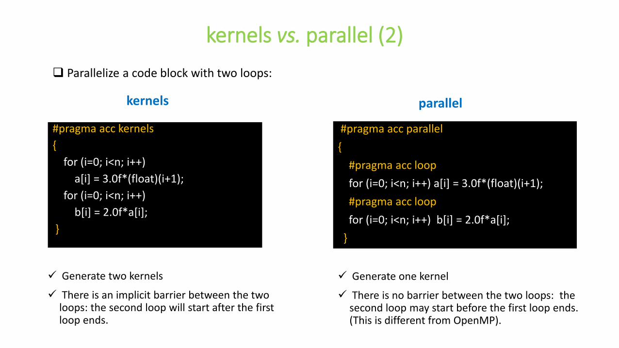
Parallelize a code block with two loops:
#pragma acc kernels
{
for (i=0; i<n; i++)
a[i] = 3.0f*(float)(i+1);
for (i=0; i<n; i++)
b[i] = 2.0f*a[i];
}
Generate two kernels
There is an implicit barrier between the two loops: the second loop will start after the first loop ends.
#pragma acc parallel
{
#pragma acc loop
for (i=0; i<n; i++) a[i] = 3.0f*(float)(i+1);
#pragma acc loop
for (i=0; i<n; i++) b[i] = 2.0f*a[i];
}
kernels parallel
Generate one kernel
There is no barrier between the two loops: the second loop may start before the first loop ends. (This is different from OpenMP).
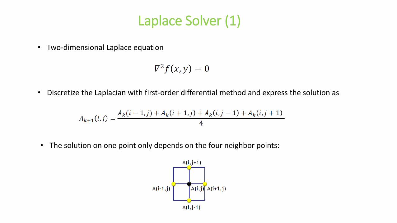
Laplace Solver (1)
• Two-dimensional Laplace equation
• The solution on one point only depends on the four neighbor points:
• Discretize the Laplacian with first-order differential method and express the solution as
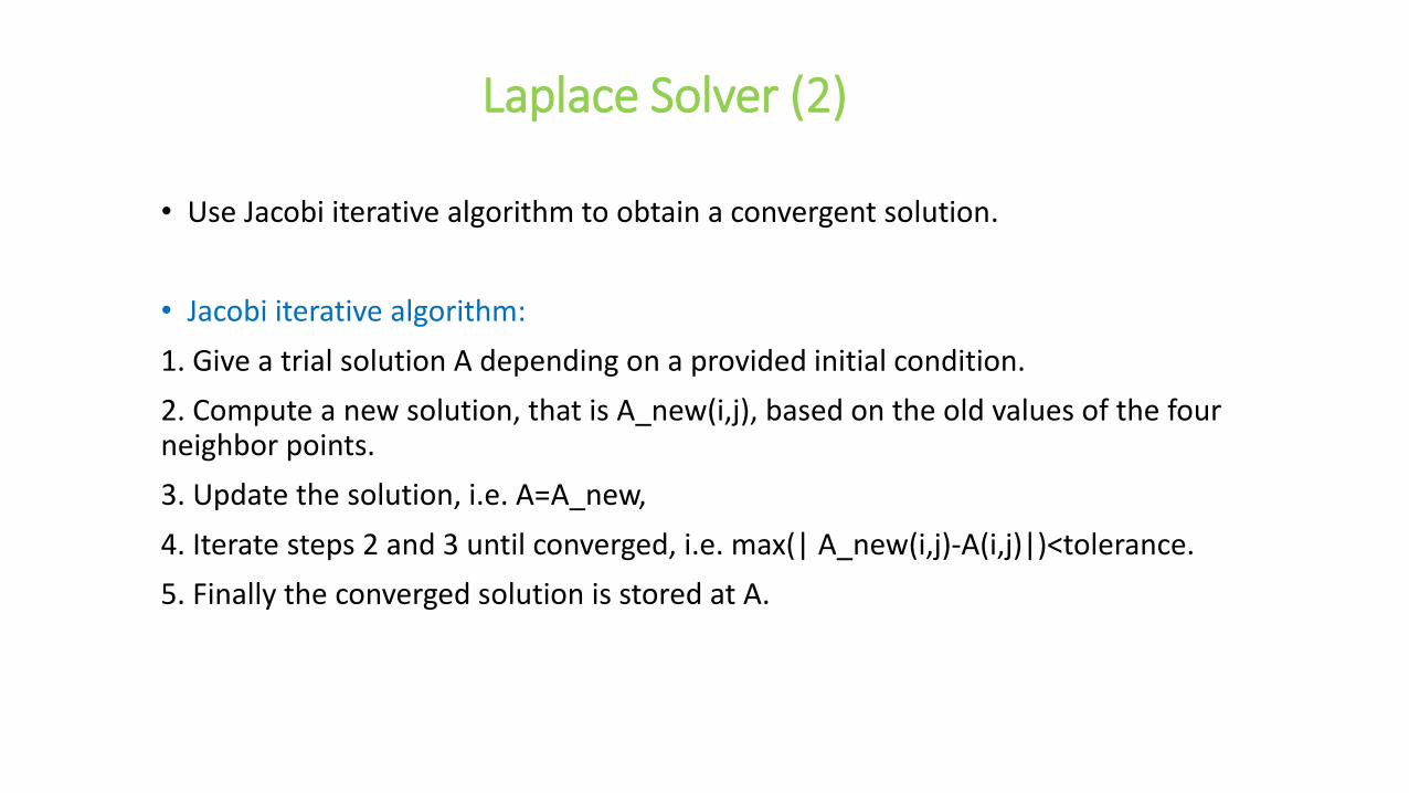
• Use Jacobi iterative algorithm to obtain a convergent solution.
• Jacobi iterative algorithm:
1. Give a trial solution A depending on a provided initial condition.
2. Compute a new solution, that is A_new(i,j), based on the old values of the four neighbor points.
3. Update the solution, i.e. A=A_new,
4. Iterate steps 2 and 3 until converged, i.e. max(| A_new(i,j)-A(i,j)|)<tolerance.
5. Finally the converged solution is stored at A.
Laplace Solver (2)
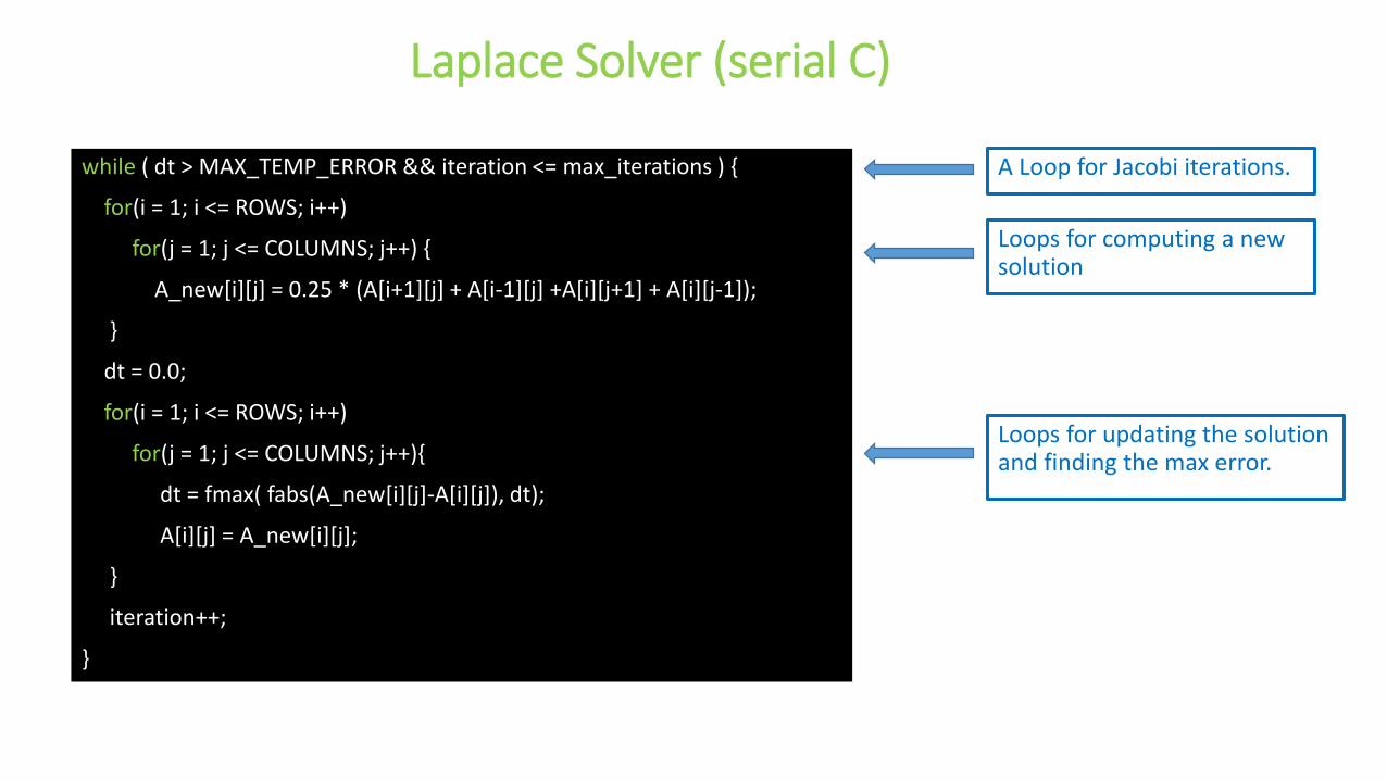
Laplace Solver (serial C)
Loops for computing a new solution
while ( dt > MAX_TEMP_ERROR && iteration <= max_iterations ) {
for(i = 1; i <= ROWS; i++)
for(j = 1; j <= COLUMNS; j++) {
A_new[i][j] = 0.25 * (A[i+1][j] + A[i-1][j] +A[i][j+1] + A[i][j-1]);
}
dt = 0.0;
for(i = 1; i <= ROWS; i++)
for(j = 1; j <= COLUMNS; j++){
dt = fmax( fabs(A_new[i][j]-A[i][j]), dt);
A[i][j] = A_new[i][j];
}
iteration++;
}
Loops for updating the solution and finding the max error.
A Loop for Jacobi iterations.
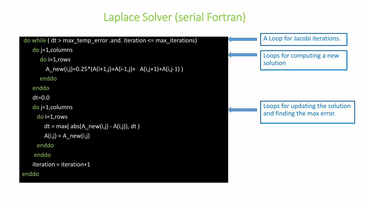
Laplace Solver (serial Fortran)
Loops for computing a new solution
do while ( dt > max_temp_error .and. iteration <= max_iterations)
do j=1,columns
do i=1,rows
A_new(i,j)=0.25*(A(i+1,j)+A(i-1,j)+ A(i,j+1)+A(i,j-1) )
enddo
enddo
dt=0.0
do j=1,columns
do i=1,rows
dt = max( abs(A_new(i,j) - A(i,j)), dt )
A(i,j) = A_new(i,j)
enddo
enddo
iteration = iteration+1
enddo
Loops for updating the solution and finding the max error.
A Loop for Jacobi iterations.
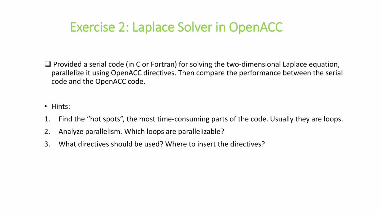
Exercise 2: Laplace Solver in OpenACC
Provided a serial code (in C or Fortran) for solving the two-dimensional Laplace equation, parallelize it using OpenACC directives. Then compare the performance between the serial code and the OpenACC code.
• Hints:
1. Find the “hot spots”, the most time-consuming parts of the code. Usually they are loops.
2. Analyze parallelism. Which loops are parallelizable?
3. What directives should be used? Where to insert the directives?
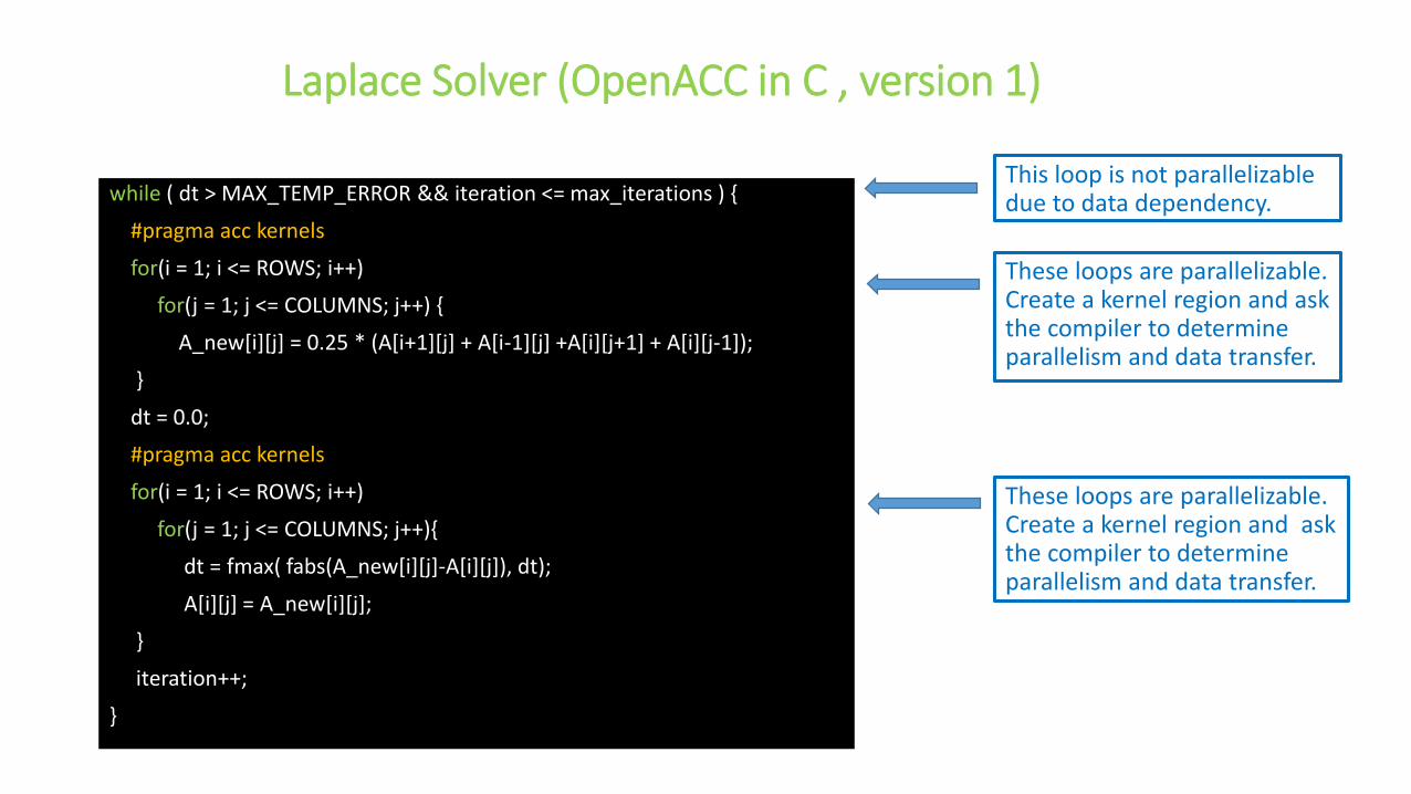
Laplace Solver (OpenACC in C , version 1)
These loops are parallelizable. Create a kernel region and ask the compiler to determine parallelism and data transfer.
while ( dt > MAX_TEMP_ERROR && iteration <= max_iterations ) {
#pragma acc kernels
for(i = 1; i <= ROWS; i++)
for(j = 1; j <= COLUMNS; j++) {
A_new[i][j] = 0.25 * (A[i+1][j] + A[i-1][j] +A[i][j+1] + A[i][j-1]);
}
dt = 0.0;
#pragma acc kernels
for(i = 1; i <= ROWS; i++)
for(j = 1; j <= COLUMNS; j++){
dt = fmax( fabs(A_new[i][j]-A[i][j]), dt);
A[i][j] = A_new[i][j];
}
iteration++;
}
These loops are parallelizable. Create a kernel region and ask the compiler to determine parallelism and data transfer.
This loop is not parallelizable due to data dependency.
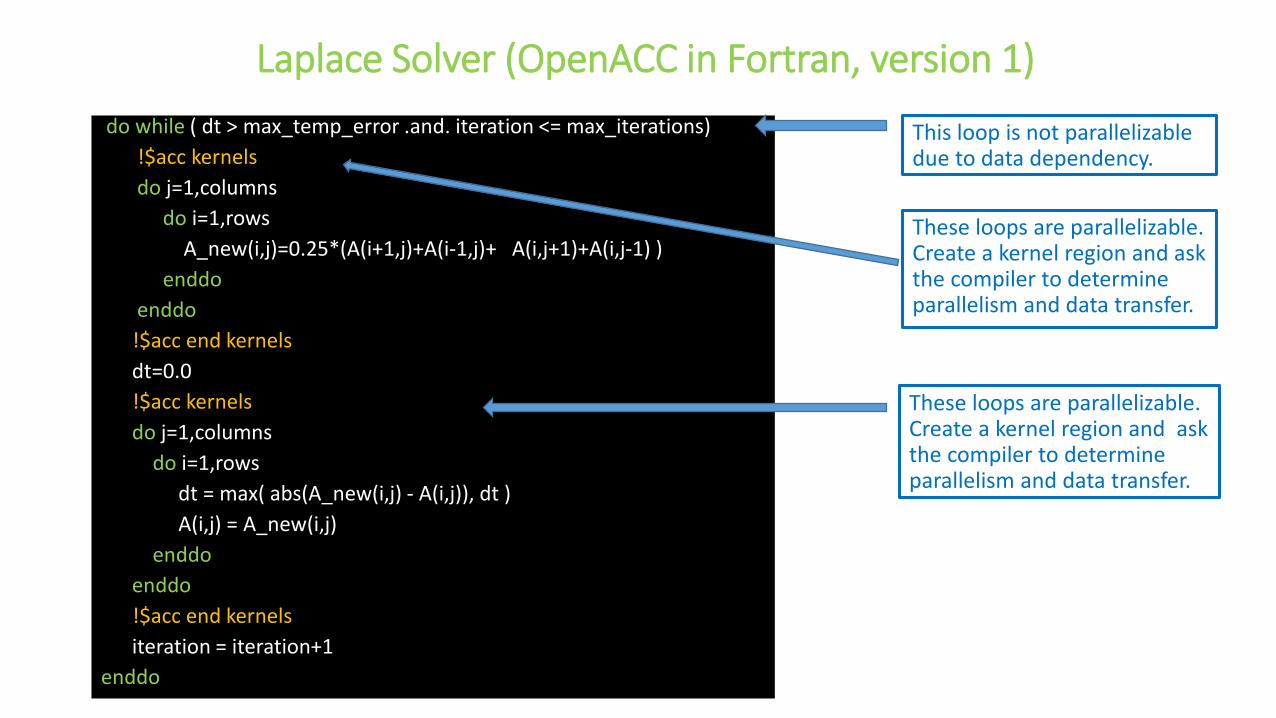
Laplace Solver (OpenACC in Fortran, version 1)
These loops are parallelizable. Create a kernel region and ask the compiler to determine parallelism and data transfer.
do while ( dt > max_temp_error .and. iteration <= max_iterations)
!$acc kernels
do j=1,columns
do i=1,rows
A_new(i,j)=0.25*(A(i+1,j)+A(i-1,j)+ A(i,j+1)+A(i,j-1) )
enddo
enddo
!$acc end kernels
dt=0.0
!$acc kernels
do j=1,columns
do i=1,rows
dt = max( abs(A_new(i,j) - A(i,j)), dt )
A(i,j) = A_new(i,j)
enddo
enddo
!$acc end kernels
iteration = iteration+1
enddo
These loops are parallelizable. Create a kernel region and ask the compiler to determine parallelism and data transfer.
This loop is not parallelizable due to data dependency.
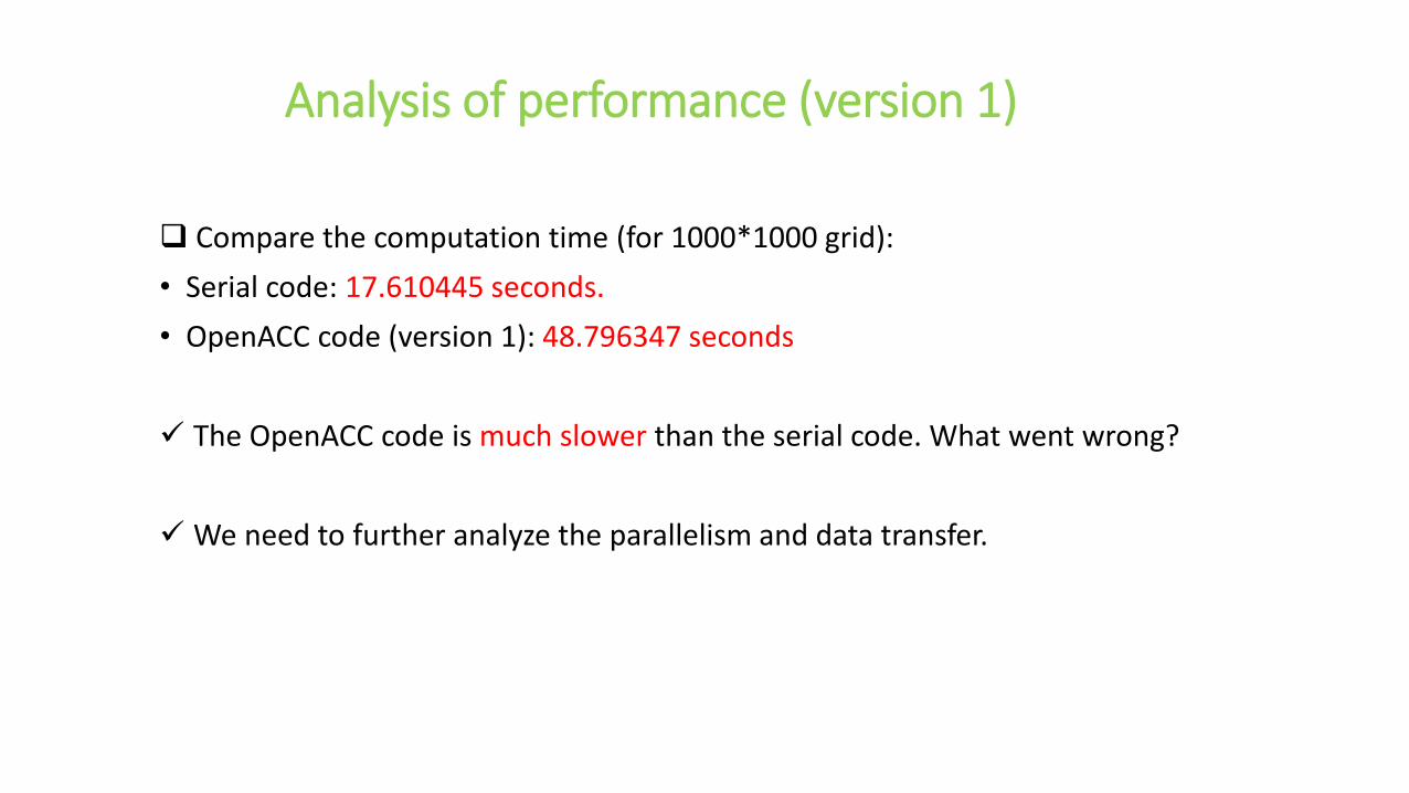
Analysis of performance (version 1)
Compare the computation time (for 1000*1000 grid):
• Serial code: 17.610445 seconds.
• OpenACC code (version 1): 48.796347 seconds
The OpenACC code is much slower than the serial code. What went wrong?
We need to further analyze the parallelism and data transfer.
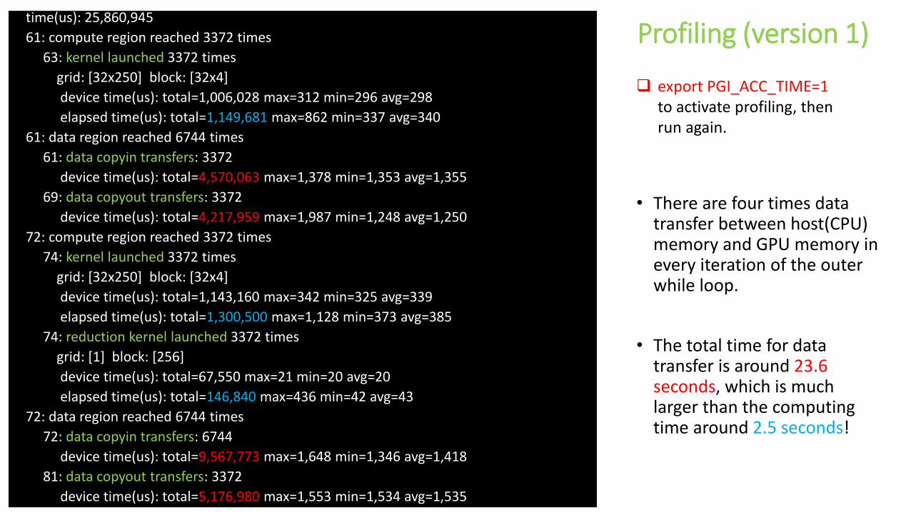
Profiling (version 1)
• There are four times data transfer between host(CPU) memory and GPU memory in every iteration of the outer while loop.
• The total time for data transfer is around 23.6 seconds, which is much larger than the computing time around 2.5 seconds!
time(us): 25,860,945
61: compute region reached 3372 times
63: kernel launched 3372 times
grid: [32x250] block: [32x4]
device time(us): total=1,006,028 max=312 min=296 avg=298
elapsed time(us): total=1,149,681 max=862 min=337 avg=340
61: data region reached 6744 times
61: data copyin transfers: 3372
device time(us): total=4,570,063 max=1,378 min=1,353 avg=1,355
69: data copyout transfers: 3372
device time(us): total=4,217,959 max=1,987 min=1,248 avg=1,250
72: compute region reached 3372 times
74: kernel launched 3372 times
grid: [32x250] block: [32x4]
device time(us): total=1,143,160 max=342 min=325 avg=339
elapsed time(us): total=1,300,500 max=1,128 min=373 avg=385
74: reduction kernel launched 3372 times
grid: [1] block: [256]
device time(us): total=67,550 max=21 min=20 avg=20
elapsed time(us): total=146,840 max=436 min=42 avg=43
72: data region reached 6744 times
72: data copyin transfers: 6744
device time(us): total=9,567,773 max=1,648 min=1,346 avg=1,418
81: data copyout transfers: 3372
device time(us): total=5,176,980 max=1,553 min=1,534 avg=1,535
export PGI_ACC_TIME=1 to activate profiling, then run again.
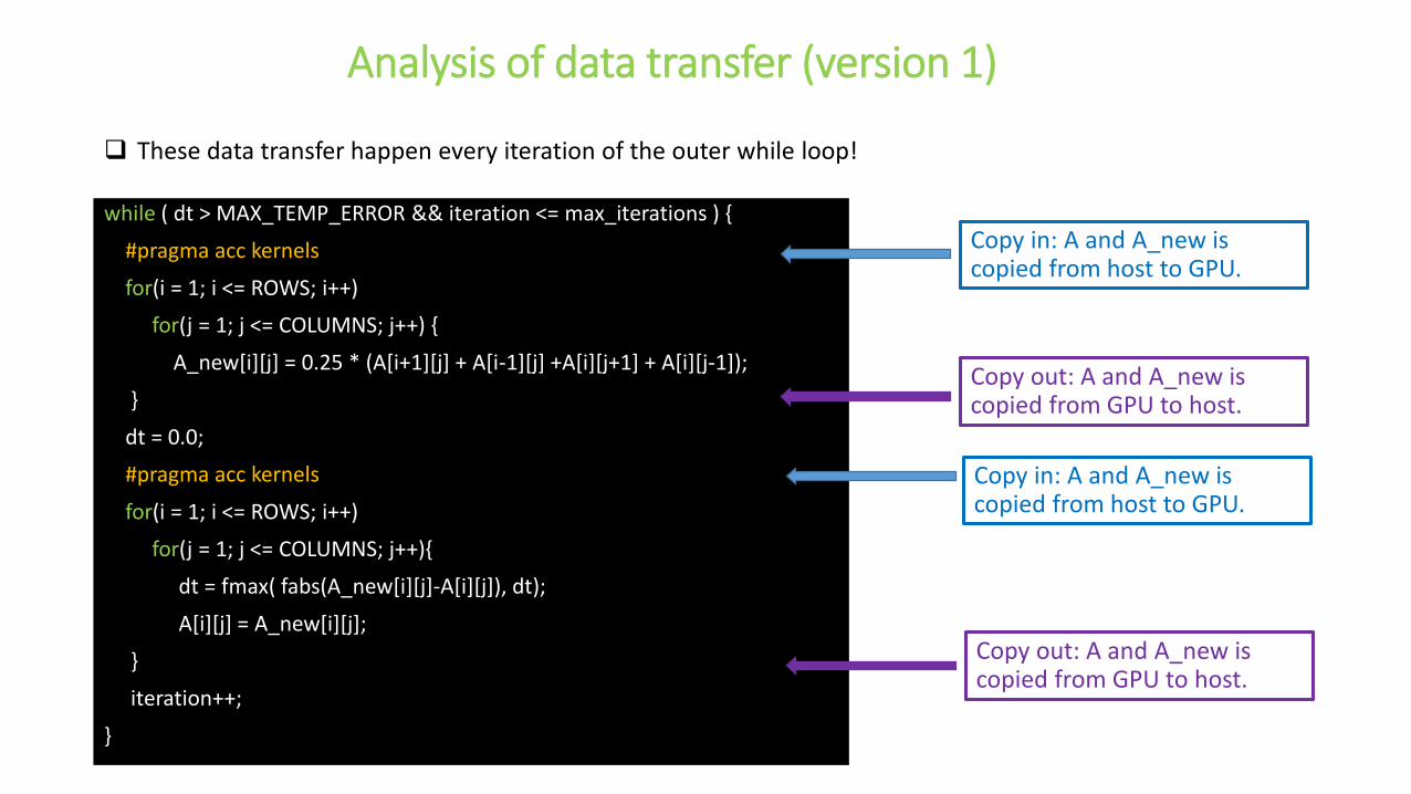
Analysis of data transfer (version 1)
Copy in: A and A_new is copied from host to GPU.
while ( dt > MAX_TEMP_ERROR && iteration <= max_iterations ) {
#pragma acc kernels
for(i = 1; i <= ROWS; i++)
for(j = 1; j <= COLUMNS; j++) {
A_new[i][j] = 0.25 * (A[i+1][j] + A[i-1][j] +A[i][j+1] + A[i][j-1]);
}
dt = 0.0;
#pragma acc kernels
for(i = 1; i <= ROWS; i++)
for(j = 1; j <= COLUMNS; j++){
dt = fmax( fabs(A_new[i][j]-A[i][j]), dt);
A[i][j] = A_new[i][j];
}
iteration++;
}
Copy out: A and A_new is copied from GPU to host.
Copy in: A and A_new is copied from host to GPU.
Copy out: A and A_new is copied from GPU to host.
These data transfer happen every iteration of the outer while loop!

Data clauses
copy (list): Allocates memory on GPU and copies data from host to GPU when entering region and copies data to the host when exiting region.
copyin(list): Allocates memory on GPU and copies data from host to GPU when entering region.
copyout(list): Allocates memory on GPU and copies data to the host when exiting region.
create(list): Allocates memory on GPU but does not copy.
present(list): Data is already present on GPU.
• Syntax for C
#pragma acc data copy(a[0:size]) copyin(b[0:size]), copyout(c[0:size]) create(d[0:size]) present(d[0:size])
• Syntax for Fortran
!$acc acc data copy(a(0:size)) copyin(b(0:size]), copyout(c(0:size)) create(d(0:size)) present(d(0:size))
!$acc end data
• If the compiler can determine the size of arrays, it is unnecessary to specify it explicitly.
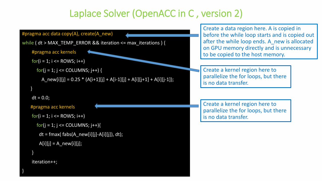
Laplace Solver (OpenACC in C , version 2)
Create a kernel region here to parallelize the for loops, but there is no data transfer.
#pragma acc data copy(A), create(A_new)
while ( dt > MAX_TEMP_ERROR && iteration <= max_iterations ) {
#pragma acc kernels
for(i = 1; i <= ROWS; i++)
for(j = 1; j <= COLUMNS; j++) {
A_new[i][j] = 0.25 * (A[i+1][j] + A[i-1][j] + A[i][j+1] + A[i][j-1]);
}
dt = 0.0;
#pragma acc kernels
for(i = 1; i <= ROWS; i++)
for(j = 1; j <= COLUMNS; j++){
dt = fmax( fabs(A_new[i][j]-A[i][j]), dt);
A[i][j] = A_new[i][j];
}
iteration++;
}
Create a data region here. A is copied in before the while loop starts and is copied out after the while loop ends. A_new is allocated on GPU memory directly and is unnecessary to be copied to the host memory.
Create a kernel region here to parallelize the for loops, but there is no data transfer.
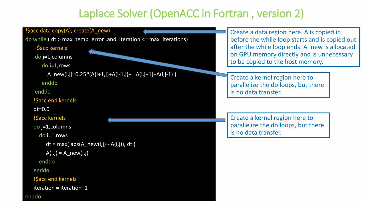
Laplace Solver (OpenACC in Fortran , version 2)
Create a kernel region here to parallelize the do loops, but there is no data transfer.
!$acc data copy(A), create(A_new)
do while ( dt > max_temp_error .and. iteration <= max_iterations)
!$acc kernels
do j=1,columns
do i=1,rows
A_new(i,j)=0.25*(A(i+1,j)+A(i-1,j)+ A(i,j+1)+A(i,j-1) )
enddo
enddo
!$acc end kernels
dt=0.0
!$acc kernels
do j=1,columns
do i=1,rows
dt = max( abs(A_new(i,j) - A(i,j)), dt )
A(i,j) = A_new(i,j)
enddo
enddo
!$acc end kernels
iteration = iteration+1
enddo
Create a data region here. A is copied in before the while loop starts and is copied out after the while loop ends. A_new is allocated on GPU memory directly and is unnecessary to be copied to the host memory.
Create a kernel region here to parallelize the do loops, but there is no data transfer.

Profiling (version 2)
• There are only 2 times data movement (of arrays) in total.
• There are data movements for the variable dt, but it not an array and thus the transfer processes cost very little time.
• The total time for data movement is around 0.09 second, which is much smaller than the computing time (around 2.5 seconds)!
time(us): 2,374,331
59: data region reached 2 times
59: data copyin transfers: 1
device time(us): total=1,564 max=1,564 min=1,564 avg=1,564
91: data copyout transfers: 1
device time(us): total=1,773 max=1,773 min=1,773 avg=1,773
63: compute region reached 3372 times
65: kernel launched 3372 times
grid: [32x250] block: [32x4]
device time(us): total=1,005,947 max=313 min=296 avg=298
elapsed time(us): total=1,102,391 max=946 min=324 avg=326
74: compute region reached 3372 times
74: data copyin transfers: 3372
device time(us): total=20,344 max=16 min=6 avg=6
76: kernel launched 3372 times
grid: [32x250] block: [32x4]
device time(us): total=1,150,552 max=344 min=327 avg=341
elapsed time(us): total=1,235,344 max=856 min=352 avg=366
76: reduction kernel launched 3372 times
grid: [1] block: [256]
device time(us): total=67,484 max=21 min=19 avg=20
elapsed time(us): total=151,147 max=358 min=43 avg=44
76: data copyout transfers: 3372
device time(us): total=68,104 max=46 min=17 avg=20
export PGI_ACC_TIME=1 to activate profiling, then run again.

Analysis of performance (version 2)
Compare the computation time (for 1000*1000 grid):
• Serial code: 17.610445 seconds.
• OpenACC code (version 1): 48.796347 seconds
• OpenACC code (version 2): 2.592581 seconds
The OpenACC code (version 2) is around 6.8 times faster than the serial code. Cheers!
The speed-up would be even larger if the size of the problem increase.
The maximum size of GPU memory (typically 6 GB or 12 GB) is much smaller than regular CPU memory (e.g. 128 GB on BU SCC).
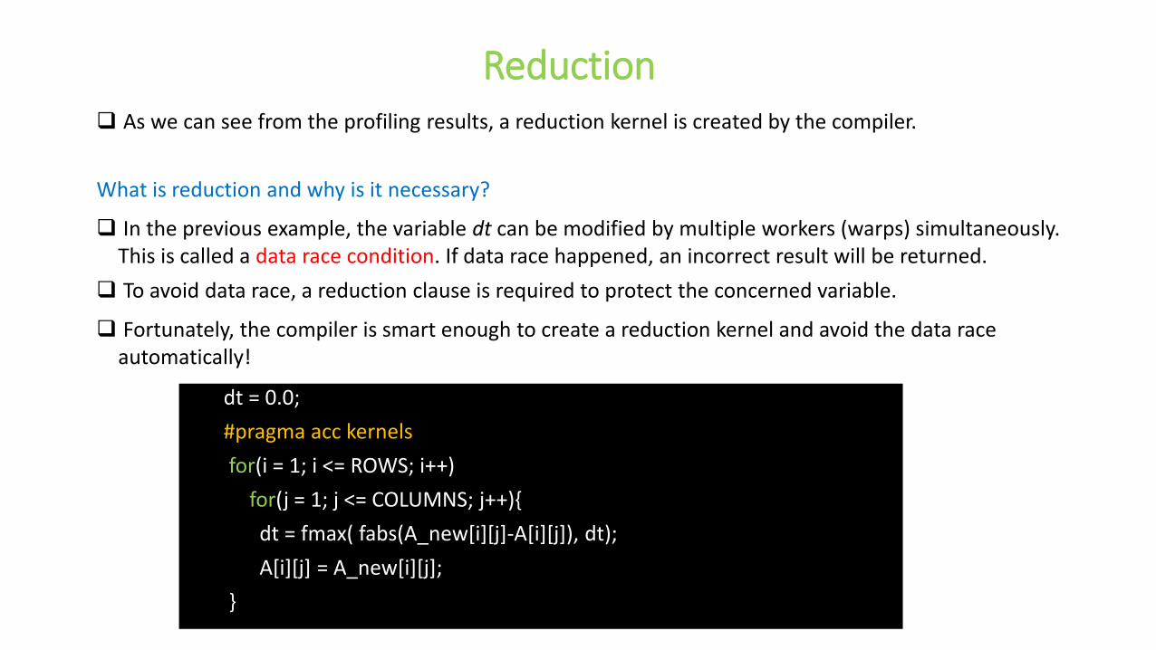
Reduction As we can see from the profiling results, a reduction kernel is created by the compiler.
What is reduction and why is it necessary?
In the previous example, the variable dt can be modified by multiple workers (warps) simultaneously. This is called a data race condition. If data race happened, an incorrect result will be returned.
To avoid data race, a reduction clause is required to protect the concerned variable.
Fortunately, the compiler is smart enough to create a reduction kernel and avoid the data race automatically!
dt = 0.0;
#pragma acc kernels
for(i = 1; i <= ROWS; i++)
for(j = 1; j <= COLUMNS; j++){
dt = fmax( fabs(A_new[i][j]-A[i][j]), dt);
A[i][j] = A_new[i][j];
}
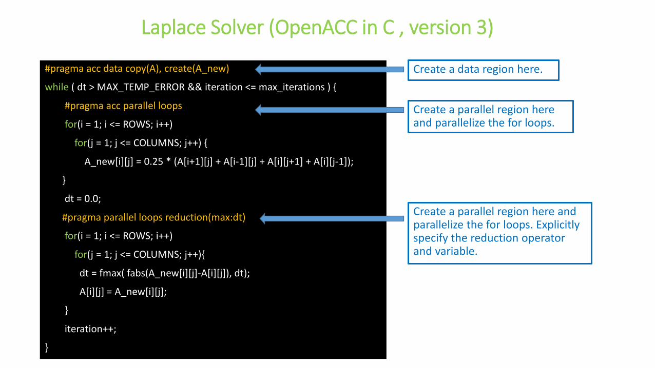
Laplace Solver (OpenACC in C , version 3)
Create a parallel region here and parallelize the for loops.
#pragma acc data copy(A), create(A_new)
while ( dt > MAX_TEMP_ERROR && iteration <= max_iterations ) {
#pragma acc parallel loops
for(i = 1; i <= ROWS; i++)
for(j = 1; j <= COLUMNS; j++) {
A_new[i][j] = 0.25 * (A[i+1][j] + A[i-1][j] + A[i][j+1] + A[i][j-1]);
}
dt = 0.0;
#pragma parallel loops reduction(max:dt)
for(i = 1; i <= ROWS; i++)
for(j = 1; j <= COLUMNS; j++){
dt = fmax( fabs(A_new[i][j]-A[i][j]), dt);
A[i][j] = A_new[i][j];
}
iteration++;
}
Create a data region here.
Create a parallel region here and parallelize the for loops. Explicitly specify the reduction operator and variable.
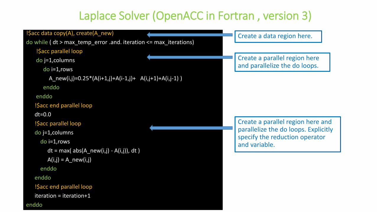
Laplace Solver (OpenACC in Fortran , version 3)
Create a parallel region here and parallelize the do loops.
!$acc data copy(A), create(A_new)
do while ( dt > max_temp_error .and. iteration <= max_iterations)
!$acc parallel loop
do j=1,columns
do i=1,rows
A_new(i,j)=0.25*(A(i+1,j)+A(i-1,j)+ A(i,j+1)+A(i,j-1) )
enddo
enddo
!$acc end parallel loop
dt=0.0
!$acc parallel loop
do j=1,columns
do i=1,rows
dt = max( abs(A_new(i,j) - A(i,j)), dt )
A(i,j) = A_new(i,j)
enddo
enddo
!$acc end parallel loop
iteration = iteration+1
enddo
Create a data region here.
Create a parallel region here and parallelize the do loops. Explicitly specify the reduction operator and variable.
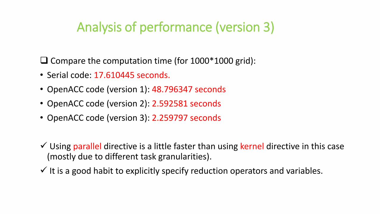
Analysis of performance (version 3)
Compare the computation time (for 1000*1000 grid):
• Serial code: 17.610445 seconds.
• OpenACC code (version 1): 48.796347 seconds
• OpenACC code (version 2): 2.592581 seconds
• OpenACC code (version 3): 2.259797 seconds
Using parallel directive is a little faster than using kernel directive in this case (mostly due to different task granularities).
It is a good habit to explicitly specify reduction operators and variables.

NVIDIA GPU (CUDA) Task Granularity
• GPU device -- CUDA grids:
Kennels/grids are assigned to a device.
• Streaming Multiprocessor (SM) -- CUDA thread blocks:
Blocks are assigned to a SM.
• CUDA cores -- CUDA threads:
Threads are assigned to a core.
Warp: a unit that consists of 32 threads.
Blocks are divided into warps.
The SM executes threads at warp granularity.
The warp size can be changed in the future.
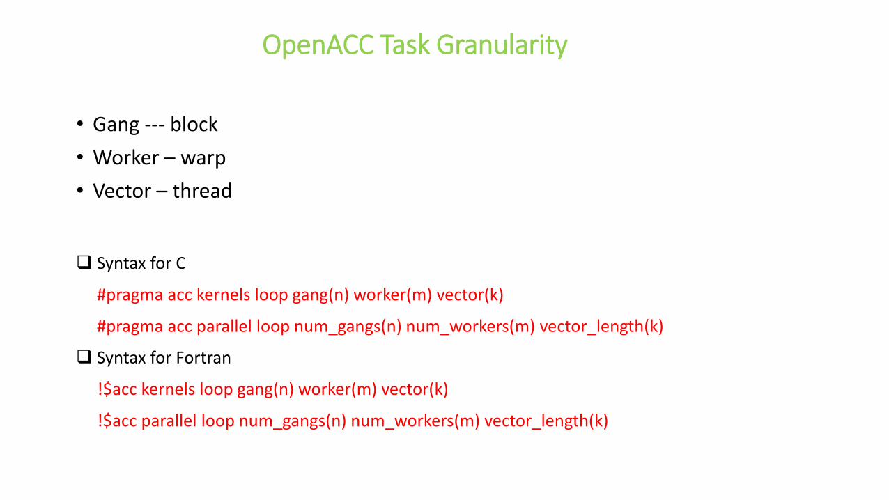
OpenACC Task Granularity
• Gang --- block
• Worker – warp
• Vector – thread
Syntax for C
#pragma acc kernels loop gang(n) worker(m) vector(k)
#pragma acc parallel loop num_gangs(n) num_workers(m) vector_length(k)
Syntax for Fortran
!$acc kernels loop gang(n) worker(m) vector(k)
!$acc parallel loop num_gangs(n) num_workers(m) vector_length(k)
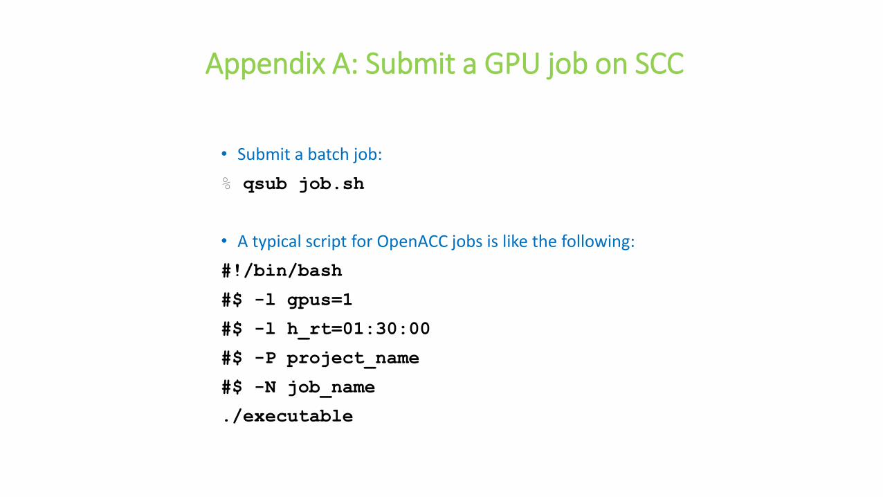
• Submit a batch job:
% qsub job.sh
• A typical script for OpenACC jobs is like the following:
#!/bin/bash
#$ -l gpus=1
#$ -l h_rt=01:30:00
#$ -P project_name
#$ -N job_name
./executable
Appendix A: Submit a GPU job on SCC
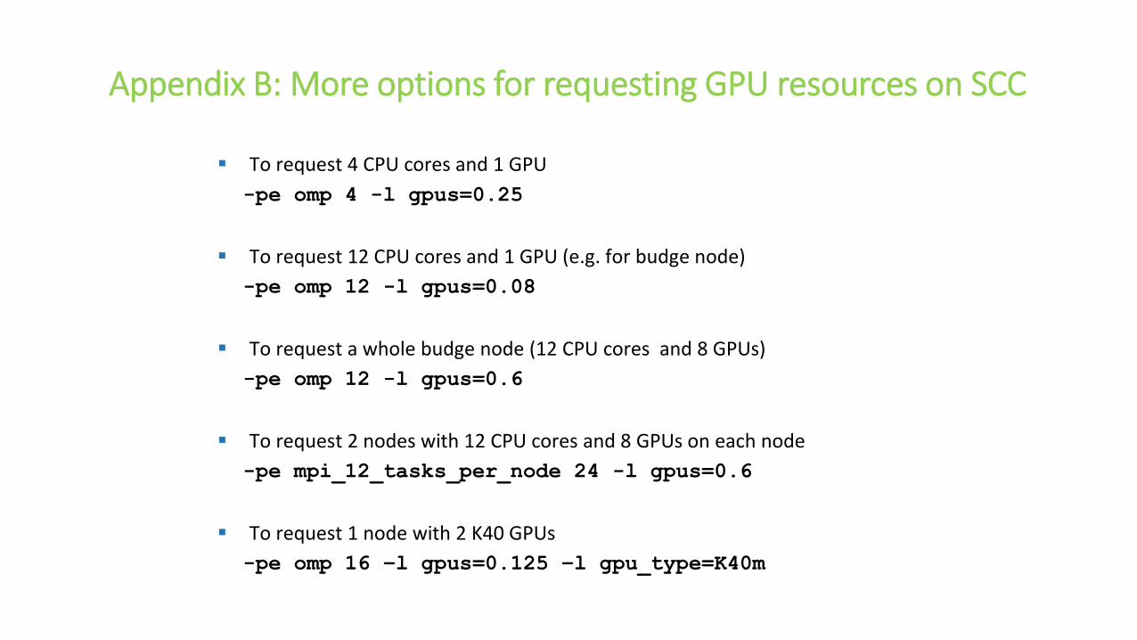
To request 4 CPU cores and 1 GPU
-pe omp 4 -l gpus=0.25
To request 12 CPU cores and 1 GPU (e.g. for budge node)
-pe omp 12 -l gpus=0.08
To request a whole budge node (12 CPU cores and 8 GPUs)
-pe omp 12 -l gpus=0.6
To request 2 nodes with 12 CPU cores and 8 GPUs on each node
-pe mpi_12_tasks_per_node 24 -l gpus=0.6
To request 1 node with 2 K40 GPUs
-pe omp 16 –l gpus=0.125 –l gpu_type=K40m
Appendix B: More options for requesting GPU resources on SCC
What is not covered
• Architecture of GPU
• Advanced OpenACC (vector, worker, gang, synchronization, etc)
• Using OpenACC with CUDA
• Using OpenACC with OpenMP (to use a few GPUs on one node)
• Using OpenACC with MPI (to use many GPUs on multiple nodes)

Further information
OpenACC official website: http://www.openacc.org/node/1
[email protected]@bu.edu


![Linux* 向けインテルの OpenCL* ツールのご紹介...Ubuntu* 14.04 CentOS* 7.2 CentOS* 7.2 Ubuntu* 14.04 Yocto* CPU GPU CPU GPU (w/ generic drive) CPU GPU [NEW] 7th Generation](https://static.fdocuments.net/doc/165x107/5e8902ca4ef530113e7b98f3/linux-fff-opencl-fffc-ubuntu-1404-centos.jpg)