Introduction to Neural Networks Daniel Kersten Lecture...

Introduction to Neural Networks

Daniel Kersten

Lecture 1-Introduction

GoalsUnderstand the functioning of the brain as a computational device. Theoretical and computational tools to explain the relationship betweenbrain & behavior. Relation to computational neuroscience and pattern recognition research, and cognitive science. Bridge mathematical levelsof analysis from the activity of single neurons to large scale systems and behavior. Examples from biological vision.

Relation to Cognitive Science and PsychologyCognitive Science is the interdisciplinary study of the acquisition, storage, retrieval and utilization of knowledge. Many disciplines involved incognitive science. Psychology is focused on understanding human behavior-- the primary motivation for the approach of this course. Problemsstudied: perception, learning, memory, decision making, reasoning, planning, action. Often, we don't know how to solve a problem even inprinciple. For others, we have solutions, but they don't resemble how a biological system might solve the problem. What kinds of problems canlarge interconnected systems of model neurons solve? What are the limitations? What are the strengths?How do neural networks relate to the larger field of statistical inference, and pattern recognition?

Understanding the relation between brain and behavior requires...A multidisciplinary approachMultiple levels of abstraction and explanation.

Multidisciplinary approachThree primary areas or disciplines influence current neural network research:

Neuroscience -> computational neuroscienceUnderstand the basic building blocks, the "hardware" or “wetware” of the nervous system

these are: nerve cells or neurons, and their connections, the synapsesExplanations and models can be quite complex. Our emphasis is on: large scale neural networks. Requires great simplification in the model ofthe neuron...in order to compute and theorize about what large numbers of them can do.Compare with other areas of Computational Neuroscience that emphasize the biology. Here we emphasize relationg neural computation tobehavior. We’ll see how statistical theories of inference, algorithms, help to provide the links from neurons to behavior. Often wrong in detail,but driven by a curiosity about how the complex processes of perception, and memory work. What can these large scale neural systems do?That is, what can they compute? And how?Computational theory -> mathematics, statistical pattern recognitionStatistical inference, engineering (information and communication theory), statistical physics and computer science. Provides the tools andanalogs to abstract and formalize for analysis and simulation. One of the characteristics of this course is to try to relate the neural models to statistical methods of inference (classification, regression,hypothesis testing) in order to understand the computational principles and power behind a neural implementation. What are the ways in whichinformation is represented? How can a system be designed to get from input to output representations?Behavioral sciences -> psychology, behavioral neuroscience, ethologyUnderstand what subsystems are supposed to do as a functioning organism in the environment. Experimental studies of perception, cognition inanimals and humans.Psychology & Computational theory =>The brain is NOT a general purpose computer.

How do different theoretical neural network approaches relate? A little history and future...

Statistical patternrecognition /∕machine

learning-−-−behavioral /∕ functional tests

Computationalneuroscience-−-−

neural tests

1950s Present ?

Multiple levels of explanationLevels of abstraction in theory development. Involve a range of spatial scales (next main section).

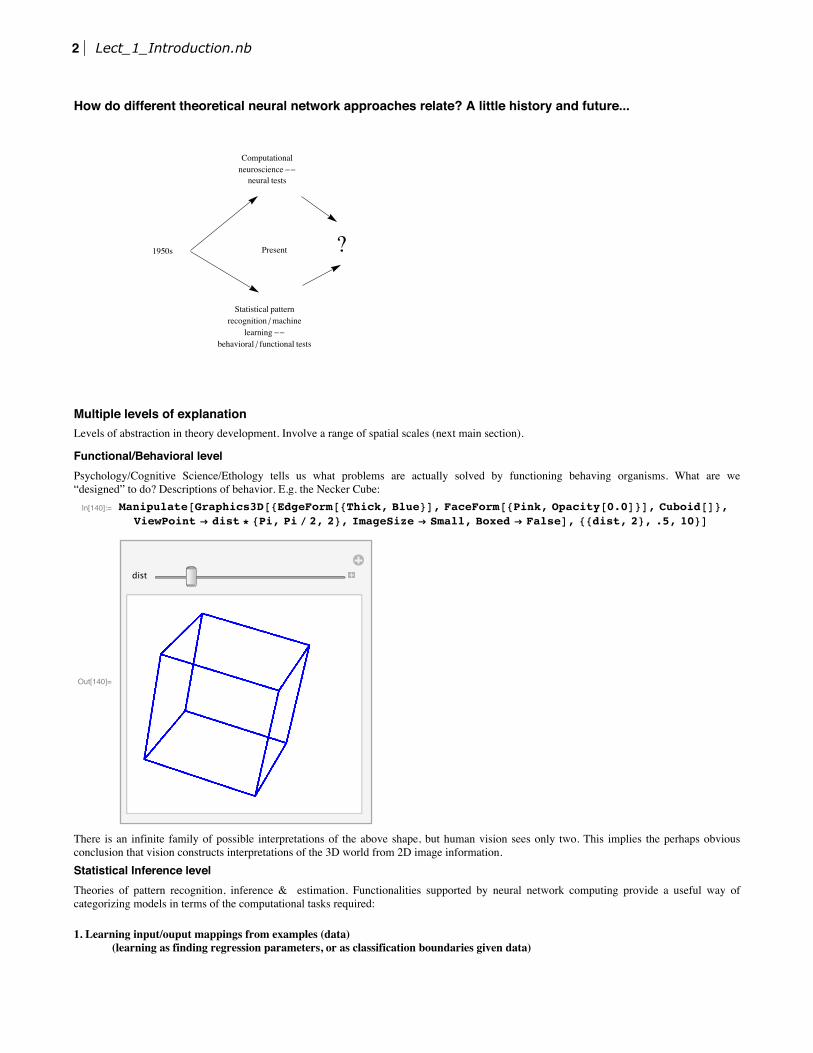
Functional/Behavioral levelPsychology/Cognitive Science/Ethology tells us what problems are actually solved by functioning behaving organisms. What are we“designed” to do? Descriptions of behavior. E.g. the Necker Cube:

In[140]:= Manipulate[Graphics3D[{EdgeForm[{Thick, Blue}], FaceForm[{Pink, Opacity[0.0]}], Cuboid[]},ViewPoint → dist *⋆ {Pi, Pi /∕ 2, 2}, ImageSize → Small, Boxed → False], {{dist, 2}, .5, 10}]

Out[140]=

dist

There is an infinite family of possible interpretations of the above shape, but human vision sees only two. This implies the perhaps obviousconclusion that vision constructs interpretations of the 3D world from 2D image information. Statistical Inference levelTheories of pattern recognition, inference & estimation. Functionalities supported by neural network computing provide a useful way ofcategorizing models in terms of the computational tasks required:

1. Learning input/ouput mappings from examples (data)(learning as finding regression parameters, or as classification boundaries given data)

2 Lect_1_Introduction.nb

1. Learning input/ouput mappings from examples (data)(learning as finding regression parameters, or as classification boundaries given data)

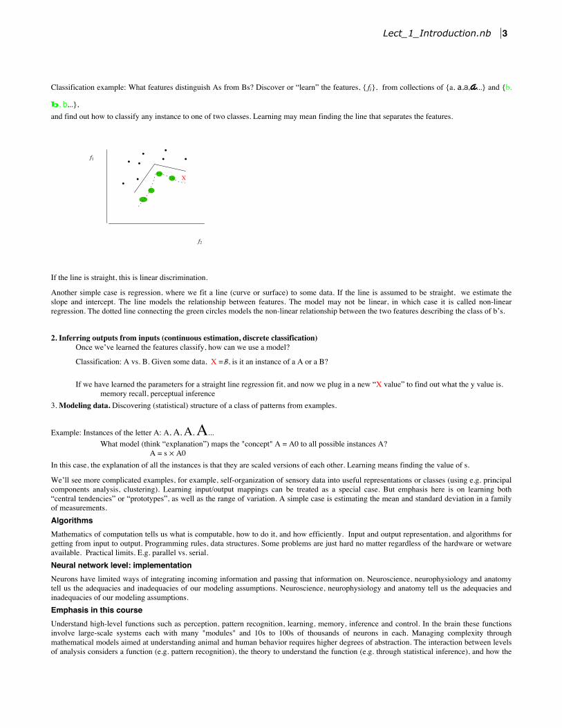
Classification example: What features distinguish As from Bs? Discover or “learn” the features, { fi}, from collections of {a, a,a,a...} and {b,

b, b,..}, and find out how to classify any instance to one of two classes. Learning may mean finding the line that separates the features.

f2

f1

X

If the line is straight, this is linear discrimination.

Another simple case is regression, where we fit a line (curve or surface) to some data. If the line is assumed to be straight, we estimate theslope and intercept. The line models the relationship between features. The model may not be linear, in which case it is called non-linearregression. The dotted line connecting the green circles models the non-linear relationship between the two features describing the class of b’s.

2. Inferring outputs from inputs (continuous estimation, discrete classification)Once we’ve learned the features classify, how can we use a model?

Classification: A vs. B. Given some data, X =B, is it an instance of a A or a B?

If we have learned the parameters for a straight line regression fit, and now we plug in a new “X value” to find out what the y value is.memory recall, perceptual inference

3. Modeling data. Discovering (statistical) structure of a class of patterns from examples.

Example: Instances of the letter A: A, A, A, A...What model (think “explanation”) maps the "concept" A = A0 to all possible instances A?

A = s × A0In this case, the explanation of all the instances is that they are scaled versions of each other. Learning means finding the value of s.

We’ll see more complicated examples, for example, self-organization of sensory data into useful representations or classes (using e.g. principalcomponents analysis, clustering). Learning input/output mappings can be treated as a special case. But emphasis here is on learning both“central tendencies” or “prototypes”, as well as the range of variation. A simple case is estimating the mean and standard deviation in a familyof measurements. AlgorithmsMathematics of computation tells us what is computable, how to do it, and how efficiently. Input and output representation, and algorithms forgetting from input to output. Programming rules, data structures. Some problems are just hard no matter regardless of the hardware or wetwareavailable. Practical limits. E.g. parallel vs. serial.Neural network level: implementationNeurons have limited ways of integrating incoming information and passing that information on. Neuroscience, neurophysiology and anatomytell us the adequacies and inadequacies of our modeling assumptions. Neuroscience, neurophysiology and anatomy tell us the adequacies andinadequacies of our modeling assumptions.Emphasis in this courseUnderstand high-level functions such as perception, pattern recognition, learning, memory, inference and control. In the brain these functionsinvolve large-scale systems each with many "modules" and 10s to 100s of thousands of neurons in each. Managing complexity throughmathematical models aimed at understanding animal and human behavior requires higher degrees of abstraction. The interaction between levelsof analysis considers a function (e.g. pattern recognition), the theory to understand the function (e.g. through statistical inference), and how thefunction may be realized in a neural system (neural networks):

Lect_1_Introduction.nb 3

Understand high-level functions such as perception, pattern recognition, learning, memory, inference and control. In the brain these functionsinvolve large-scale systems each with many "modules" and 10s to 100s of thousands of neurons in each. Managing complexity throughmathematical models aimed at understanding animal and human behavior requires higher degrees of abstraction. The interaction between levelsof analysis considers a function (e.g. pattern recognition), the theory to understand the function (e.g. through statistical inference), and how thefunction may be realized in a neural system (neural networks):

The Big Picture: Overview of the BrainBefore we look at models of neurons and their interactions, let us get an overview of the large scale context.

Understanding function means understanding how an organism's information processing is determined by the structure of its environmentalinputs (e.g. natural images, objects to be avoided, places to go), and the nature of its outputs (e.g. estimates of shapes of objects to be manipu-lated, terrain to walk on, movements, and decisions). The brain doesn't operate in isolation, these inputs and outputs are intimately tied to thesensory and motor neurons that make up the peripheral nervous system, as well as the physical make-up of the body itself.

The brain has both surface and interior structures. Surface structures that are visible in the side view below are: frontal, temporal, parietal andoccipital lobes, and the cerebellum. But apart from the cerebellum, it isn't totally obvious where one part stops and another begins. Landmarksare the sulci (valleys) and gyri (bumps). E.g. the lateral fissure (sulcus) is perhaps the easiest to spot. It separates the temporal lobe from thefrontal and parietal lobes. There are internal components too: Thalamus (sensory and motor relays), hypothalamus (control of endocrineactivity, temperature, food intake, etc..), basal ganglia (motor behavior, habits), limbic system (emotion), medulla (part of lower brain stem,breathing, heart rate). We believe that much of what makes us interesting as humans, our thoughts, imaginations, words and actions, depends onhaving a large and complex cortex. A common view shows the surface or cortex--the gray matter.

From: http://www.utdallas.edu/~kilgard/brain.jpg

Check out: http://culhamlab.ssc.uwo.ca/fmri4newbies/

The anatomy provides an important, but static view of the brain. Progress in functional imaging provides dynamic pictures that illustraterelationships between human functions (seeing, imagining, etc.) are related to various cortical areas. (From an early example from our own lab, see: http://gandalf.psych.umn.edu/users/kersten/kersten-lab/Perceptual.html)


Multiple levels of organization: spatial and temporal scales

From: Churchland & Sejnowski. (10,000 A to a micron)

Example: Visual systemLet's take a look from two points of view: 1) information flow through a specific system--the visual system; 2) levels of organization atsuccessive stages. At a very coarse spatial scale, we know that we have eyes and a portion of the brain that processes the incoming images. This system enables usto manipulate objects, to navigate, to recognize and think and talk about objects, their attributes and relations.


Anatomical view of a system

(From wikipedia entry for "Visual System")

The above picture ends at primary visual cortex (V1, area 17), but there are more than 30 other visual areas after that.

Spatial scales of the visual cortex: hierarchical organization (~ 10 cm scale), areas or “maps” (~ 1 cm scale), Higher visual areas in cortex.


From: Tootell, R. B., Tsao, D., & Vanduffel, W. (2003). Neuroimaging weighs in: humans meet macaques in "primate" visual cortex. J Neurosci, 23(10), 3981-3989.

Image[ ]

From: Wallisch, P., & Movshon, J. A. (2008). Structure and Function Come Unglued in the Visual Cortex. Neuron, 60(2), 194–197.doi:10.1016/j.neuron.2008.10.008

Cortical layers & circuits (~ 1 mm scale)Structure within maps do not consist of randomly connected nerve cells. There is a medium-level organization into multiple functionalgroupings. The neocortex has 6 more or less distinguishable layers, there is a microorganization into vertical columns. In the primary visualcortical area (V1, see above figure), there are ocular dominance and orientation selectivity columns which are believed to form a functional unitcalled a hypercolumn (1 to 2 mm). Each hypercolumn takes into account local image intensities and colors to represent information or featuresfor a single point of the visual field.


http://www.ualr.edu/~klwennstrom/hypercolumn.gif

Image[ ]

The above figure illustrates some cell types in layers of gray matter.

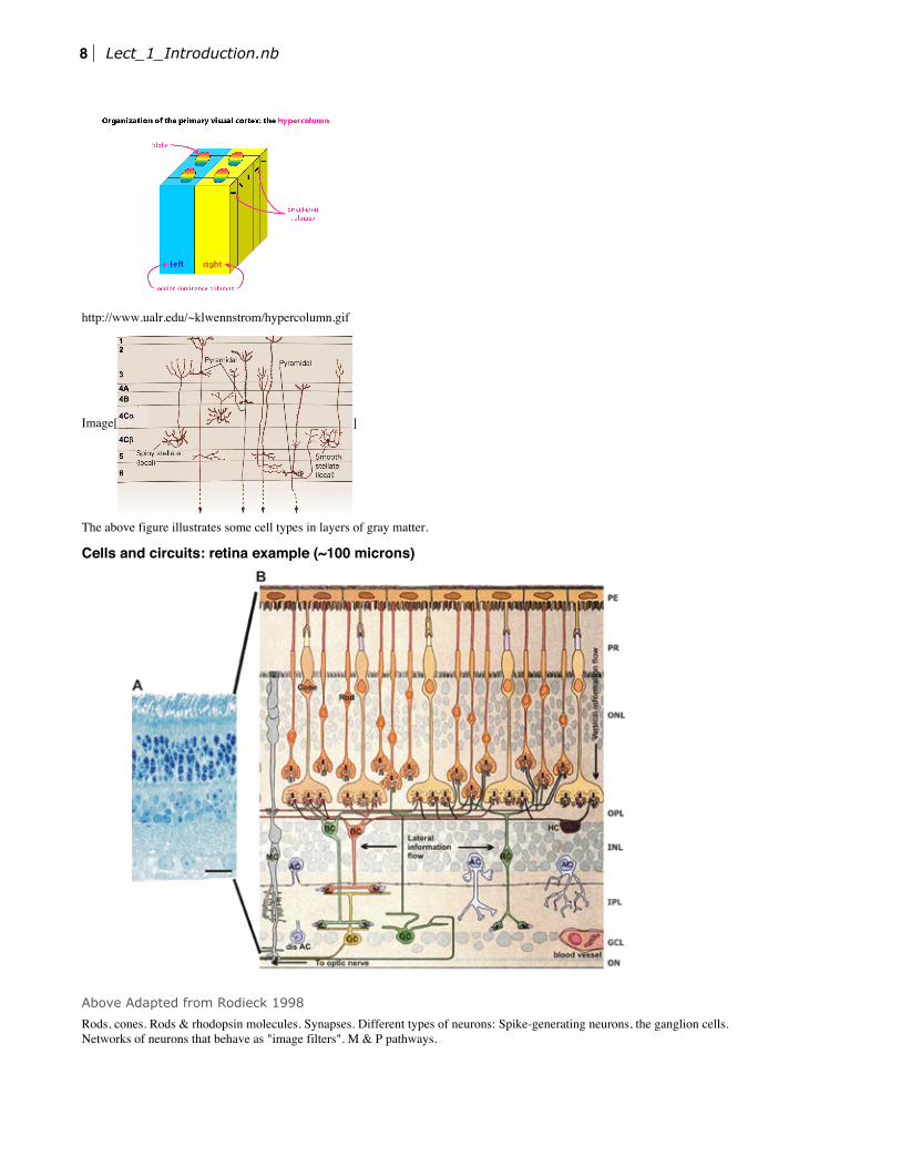
Cells and circuits: retina example (~100 microns)

Above Adapted from Rodieck 1998Rods, cones. Rods & rhodopsin molecules. Synapses. Different types of neurons: Spike-generating neurons, the ganglion cells.Networks of neurons that behave as "image filters". M & P pathways.

Image[ ]


Image[ ]

Retinal “J cell”: http://blog.eyewire.org/twos-company/

Temporal, functional view of a process On the spatial scales of 1 to 10 to 50 cm, and time scale of a 1/4 of a second and less.

(example from Simon Thorpe's lab: http://www.cerco.ups-tlse.fr/Simon-THORPE?lang=en)

An example of a model based on the hierarchical structure of the ventral visual stream. On the order of 1 mm to 10 cm.


From Serre, T., Oliva, A., & Poggio, T. (2007). A feedforward architecture accounts for rapid categorization. Proc Natl Acad Sci U SA, 104(15), 6424-6429.

Some brain specsThe human brain is:: volume - 1.4 liters, Cortex 2 mm, volume 0.32 litersCortex: 1.6 x 10^10 neurons, with an average of about 4000 synapses/neuron, about 6x10^13 connections.Area of cortex 1.60 E + 05 mm^2Thickness of cortex 2.00 E + 00 mmVolume of cortex 3.20 E + 05 mm^3 3.20 E -− 01 litersCortex synapse density 4.00 E + 03 synapse/∕neuronCortex connectivity 2.00 E + 08 synapses/∕mm^3connectivity/∕neuron 5.00 E + 00 mmconnection length/∕mm^3 2.50 E + 04 mmneuron density in cortex 5.00 E + 04 neurons/∕mm^3Total brain volume 1.40 E + 00 litersTotal neurons in cortex 1.60 E + 10Total visual neurons 8.00 E + 09

(50 % visual neurons is often quoted and used here,but is difficult to pin down)

Total visual connection lengths 4.00 E + 09 mm4.00 E + 07 m or 24 874 miles of connections

(about the distance around the earth at the equator, 24, 901 miles)

Some reference numbers taken or inferred from those published by :Cherniak, J. of Cog. Neurosc., 1990, vol 2., pp 58 -− 68

Getting started with MathematicaMathematica vs. Matlab vs. Python vs. dedicated neural network simulation packages.


Front-end and Notebooks: Organize, outline, document. Program, evaluations, data all in one placeKernel: Separate program does the calculations

To get an overview of Mathematica and its help resources:The Wolfram Documentation window, under Help, and its search dialog box are useful to keep open for general code development

PracticeNumerical Calculations. You can do arithmetic. For example, type 5+7 as shown in the cell below, and then hit the "enter" key. Note that if youtry division, e.g. 2/3, you get the exact answer back. To get a decimal approximation, type N[2/3].

5+7

12

2 /∕ 3

2

3

N[2/∕3]

0.666667

You can go back and select an expression by clicking on the brackets on the far right. These brackets serve to organize text and calculationsinto a Notebook with outlining features. You can group or ungroup cells for text, graphs, and expressions in various ways to present yourcalculations. Explore these options under Cell in the menu. You can see the possible cell types under the Style menu.Try some other operations, 5^3, 4*3 (note that 4 3, where a space separates the digits is also interpreted as multiplication.

Evaluate 4*3

Compare with 4 3 (i.e. 4 followed by a space, and then 3).

Seems pretty dumb so far...but you can see that Mathematica's default handling of arithmetic is special:

Compare the square roots of: 12345678987654321 and 12345678987654321.0

Compare (2^.000000000001)^1000000000000 with (2^(1/1000000000000))^1000000000000

If you don't explicitly tell Mathematica that your expressions involving floating point numbers, it will treat the numbers as true integers. And ingeneral, Mathematica will do symbolic processing as a default, and assume you want as general an answer as possible. Because symbolicprocessing demands considerably more computer resources than numerical processing, this result in annoying consequences, like slow or noresponsivity. So remember to include a decimal point somewhere, or use N[] to force a floating point representation, and consequently numeri-cal computations.

Front-end stuffThere's a lot to explore stylistically in Notebooks, but one of the most common things you will do is to select and manipulate the brackets onthe far right. You can go back and select an expression by clicking on the brackets on the far right. These brackets are features of the userinterface and serve to organize text and calculations into a Notebook with outlining features. You can group or ungroup cells for text, graphs,and expressions in various ways to present your calculations. Explore these options under Cell in the menu. You can see the possible cell typesunder the Style menu.

By ending an expression with ; you can suppress the output--this is useful later when the output might be a list of a 10,000 neural activity levels!

(3/∕4)/∕6;(3 4)/∕6;

Before Mathematica 6, you had to be particularly careful... without a semi-colon before evaluating the next cell, you could end up with aNotebook full of 50,000 "hi"s:

a = Table["hi", {50 000}]


{hi, hi, hi, hi, hi, hi, hi, hi, hi, hi, hi, hi, hi, hi, hi, hi, hi, hi, hi, hi, ⋯ 49 960⋯ ,hi, hi, hi, hi, hi, hi, hi, hi, hi, hi, hi, hi, hi, hi, hi, hi, hi, hi, hi, hi}

large output show less show more show all set size limit...

The most recent result of a calculation is given by %, the one before by %%, and so forth. Try it on the previous two outputs

Built-in functionsMathematica has a very large library of built-in functions. They all begin with an uppercase letter and the arguments are enclosed by squarebrackets. Knowing that, you can often guess the form of a function.Try taking the logarithm of 8.0

Did it return log to the base 10 or e? Check the definition by typing "?Log" or by typing "Log[E]" and "Log[10]"

You can get information more about a function, by clicking on the resulting link >>

Try Log[2,8]

You can get information about a function, e.g. for the exponential of a function, or for plotting graphs by selecting the function (e.g. Exp) andgoing to "Find Selected Function" in the Help menu. Or you can enter:

?Exp

Exp[z] gives the exponential of z. #

and then click on >> to take you to the documentation page.

?Plot

Plot[ f , {x, xmin, xmax}] generates a plot of f as a function of x from xmin to xmax.Plot[{ f1, f2,…}, {x, xmin, xmax}] plots several functions fi. #

If you type two question marks before a function, ??Plot, you'll get more information. Try it. What does the Random function do?

Defining your own functionsLet's illustrate function definition by building a simple model of a neuron’s input/output function. We'll see the justification later. Suppose aneuron takes a set of inputs, say x1, x2, x3, (e.g. from the outputs of three other neurons in the network) and produces an output signal, call it y. For a so-called linear model, the output is the weighted sum of the inputs. We'll assume the weights are fixed and given by w1, w2, w3.

w1 = -−1; w2 = 2; w3 = -−1;

y[x1_, x2_, x3_] := w1 *⋆ x1 + w2 *⋆ x2 + w3 *⋆ x3;

(This code is pretty primitive and not very general--don't worry, we'll get more sophisticated later). The underscore in x1_ is important because it tells Mathematica that x1 represents a slot for a variable, not an expression. := vs. =Note that when defining a function, we used a colon followed by equals ( := ) instead of just an equals sign (=). When you use an equals sign,the value is calculated and assigned immediately. When there is a colon in front of the equals, the value is calculated only when called on later.So we use := for function definition because we need to define the function for later use and evaluation, when we may have new values for itsarguments.(A double equals (==) has yet another meaning and is used to represent a symbolic equation which evaluates to True if left and right hand sidesare identical.)Let's define xv using :=, and xf using =

In[141]:= xv := RandomInteger[10];xf = RandomInteger[10];

Now evaluate r1 and r2 three times each. What is the difference between the two definitions?


In[144]:= {xv, xf}

Out[144]= {3, 9}

..but if we evaluate xf = RandomInteger[10] again, we re-initialize it:

In[145]:= xf = RandomInteger[10]

Out[145]= 10

In[146]:= xf = RandomInteger[10];y[xf, xf, xf]

Out[147]= 0

Compare repeated evaluations of the above with repeated evaluations of the expression below.

In[149]:= y[xv, xv, xv]

Out[149]= 5

Why does our neuron model always output a zero when the inputs all have the same value? What other family of inputs will all produce zero output? Hint: The weights we defined can be thought of as a discrete approximation to a 2nd derivative operator in differential calculus.

Graphics & more function definitionsLater on we'll require defining a function that suppresses small outputs and "squashes" or clamps large outputs to a maximum level. Here is anexample:

In[150]:= squash[x_] := N[1/∕(1 + Exp[-−x+4])];

Also note that our squashing function was defined with N[]. Again, remember that Mathematica trys to keep everything exact as long aspossible and thus will try to do symbol manipulation if we don't explicitly tell it that we want numerical representations and calculations.Let's plot a graph of the squash function for -5<x<10, using the syntax we learned about above:

In[151]:= Plot[squash[x], {x, -−5, 10}]

Out[151]=

-−4 -−2 2 4 6 8 10

0.2

0.4

0.6

0.8

1.0

We'll use this and similar functions to model the small-signal compression and large signal saturation characteristics of neural output.

Define a new function squashedExp[ ] that applies squash to an exponentiated value (i.e. takes Exp[x] as the argument of squash[ ])

In[152]:= squashedExp[x_] := squash[Exp[x]];

Plot squashedExp[ ] for x going from -5 to 5

In[154]:= Plot[{Exp[x], squashedExp[x]}, {x, -−5, 5}, ImageSize → Small]

Out[154]=

-−4 -−2 2 4

2

4

6

8

10

Even though Exp grows exponentially fast with increasing x (by definition!), squash “keeps a lid” on it.


Ask Mathematica for the definition of squashedExp[ ]

It can be important to check your definitions like this. One reason is that, as we will see later, Mathematica definitions can be built up line-by-line, incorporating multiple criteria/constraints. And sometimes you might add to a function unwittingly and it appears to misbehave. You cancheck your defintion by asking Mathematica for it.Define a new version of the squash function to include a steepness term λ, and use Manipulate to control λ

In[155]:= ? squash

Mathematica has useful and easy-to-program GUI tools. One of the most common is Manipulate[]

In[156]:= dsquash[x_,λ_] := N[1/∕(1 + Exp[(-−x+4)/∕λ])];Manipulate[Plot[dsquash[x,λ], {x, -−5, 10}],{{λ,1},0.1,2}]

Out[157]=

λ𝜆

-−4 -−2 2 4 6 8 10

0.2

0.4

0.6

0.8

1.0


In[159]:= Manipulate[Plot3D[Exp[-−x^2 -− y^2] *⋆ Sin[a *⋆ x + b *⋆ y],{x, -−2, 2}, {y, -−2, 2}, PlotRange → {-−2, 2}], {a, 1, 6}, {b, 1, 6}]

Out[159]=

a

b

Try using your mouse and mouse button to rotate the above plot. What does the Option or Alt key do?

Mathematica Demonstrations project

Check out the Demonstrations center at the Wolfram Mathematica site for some cool examples, such as:


In[160]:= Manipulate[Module[{bluecol, colfunc},bluecol[n_] := Blend[{Black, Blue, White}, n];If[usecol, colfunc = bluecol, colfunc = GrayLevel];

Graphics[{colfunc[left], Rectangle[{0, 0}, {3, 3}], colfunc[right], Rectangle[{3, 0}, {6, 3}],colfunc[mid], Rectangle[{1, 1}, {2, 2}], Rectangle[{4, 1}, {5, 2}]}]],

{{left, .35, "left square"}, .2, .8}, {{right, .75, "right square"}, .2, .8},{{mid, .5, "middle squares"}, .2, .8},{{usecol, True, ""}, {True → "blues", False → "grays"}, ControlPlacement → Bottom}]

Out[160]=

left square

right square

middle squares

blues grays

"The Simultaneous Contrast Effect" from The Wolfram Demonstrations Project http://demonstrations.wolfram.com/TheSimultaneousCon-trastEffect/

Next timeBasic structure and function of a single neuron

ReferencesBear, M. F., Connors, B. W., & Paradiso, M. A. (2006). Neuroscience : exploring the brain (3rd ed.). Baltimore, MD: Lippincott Williams &Wilkins.Churchland, P. S., & Sejnowski, T. J. (1992). The Computational Brain . Cambridge, MA: MIT Press.Felleman, D. J., & Van Essen, D. C. (1991). Distributed hierarchical processing in the primate cerebral cortex. Cereb Cortex, 1(1), 1-47.Kandel, E. R., Schwartz, J. H., & Jessell, T. M. (2000). Principles of neural science (4th ed.). New York: McGraw-Hill, Health ProfessionsDivision.Levy, I., Hasson, U., & Malach, R. (2004). One picture is worth at least a million neurons. Curr Biol, 14(11), 996-1001.Milner, D., & Goodale, M. (1995). The Visual Brain in Action . Oxford: Oxford University Press.Purves, D. (2007). Neuroscience (4th ed.). Sunderland, Mass.: Sinauer Associates, Publishers.Rolls, E.T., & Treves, A. (1998). Neural networks and brain function. Oxford ; New York: Oxford University Press.Zeki, S. (1993). A Vision of the Brain. Oxford: Blackwell Scientific Publications.


Linkshttp://www.med.harvard.edu/AANLIB/cases/caseM/case.htmlhttp://thalamus.wustl.edu/course/© 1998,2001,2003,2005,2007, 2009, 2011, 2012, 2014 Daniel Kersten, Computational Vision Lab, Department of Psychology, University of Minnesota.


Introduction to Neural Networks Daniel Kersten Lecture...

Documents

Transcript of Introduction to Neural Networks Daniel Kersten Lecture...