1

Wolfram Burgard, Cyrill Stachniss,

Maren Bennewitz, Kai Arras

Probabilistic Motion Models

Introduction to Mobile Robotics

2

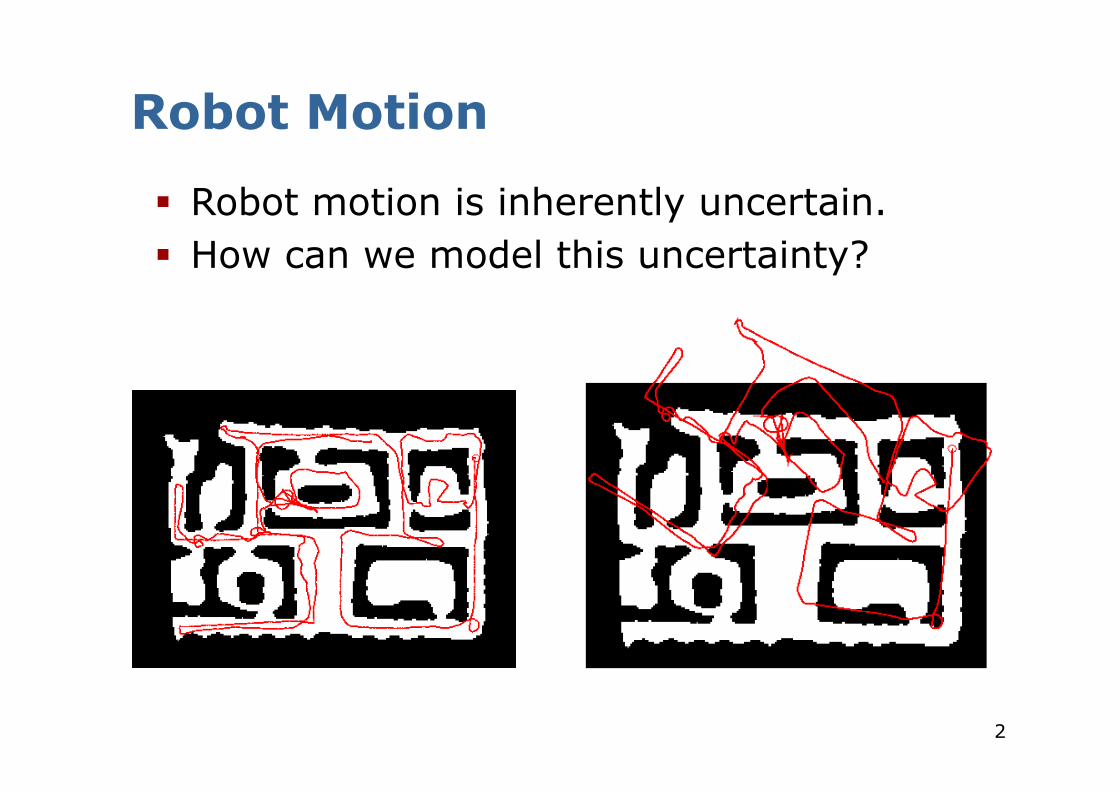
Robot Motion

§  Robot motion is inherently uncertain. §  How can we model this uncertainty?

3

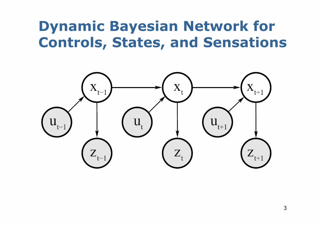
Dynamic Bayesian Network for Controls, States, and Sensations

4

Probabilistic Motion Models §  To implement the Bayes Filter, we need the

transition model p(x j x’, u).

§  The term p(x j x’, u) specifies a posterior probability, that action u carries the robot from x’ to x.

§  In this section we will specify, how p(x j x’, u) can be modeled based on the motion equations.

5

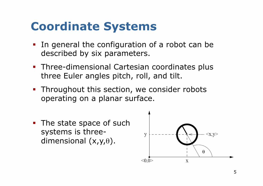
Coordinate Systems §  In general the configuration of a robot can be

described by six parameters.

§  Three-dimensional Cartesian coordinates plus three Euler angles pitch, roll, and tilt.

§  Throughout this section, we consider robots operating on a planar surface.

§  The state space of such systems is three-dimensional (x,y,θ).

6

Typical Motion Models

§  In practice, one often finds two types of motion models: §  Odometry-based §  Velocity-based (dead reckoning)

§  Odometry-based models are used when systems are equipped with wheel encoders.

§  Velocity-based models have to be applied when no wheel encoders are given.

§  They calculate the new pose based on the velocities and the time elapsed.

7

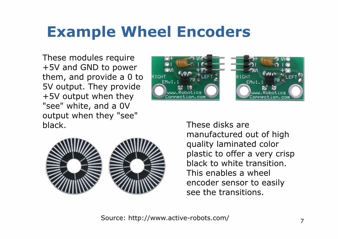
Example Wheel Encoders These modules require +5V and GND to power them, and provide a 0 to 5V output. They provide +5V output when they "see" white, and a 0V output when they "see" black. These disks are

manufactured out of high quality laminated color plastic to offer a very crisp black to white transition. This enables a wheel encoder sensor to easily see the transitions.

Source: http://www.active-robots.com/

8

Dead Reckoning

§  Derived from “deduced reckoning.” §  Mathematical procedure for determining

the present location of a vehicle. §  Achieved by calculating the current pose of

the vehicle based on its velocities and the time elapsed.

9

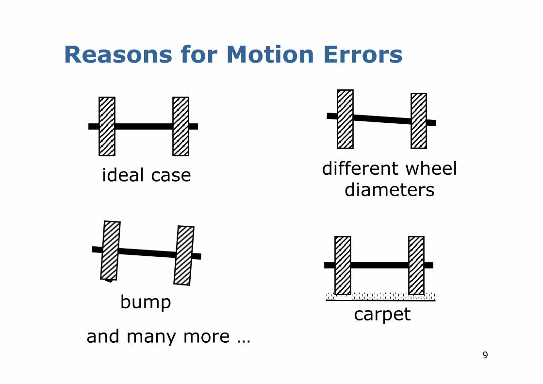
Reasons for Motion Errors

bump

ideal case different wheel diameters

carpet and many more …

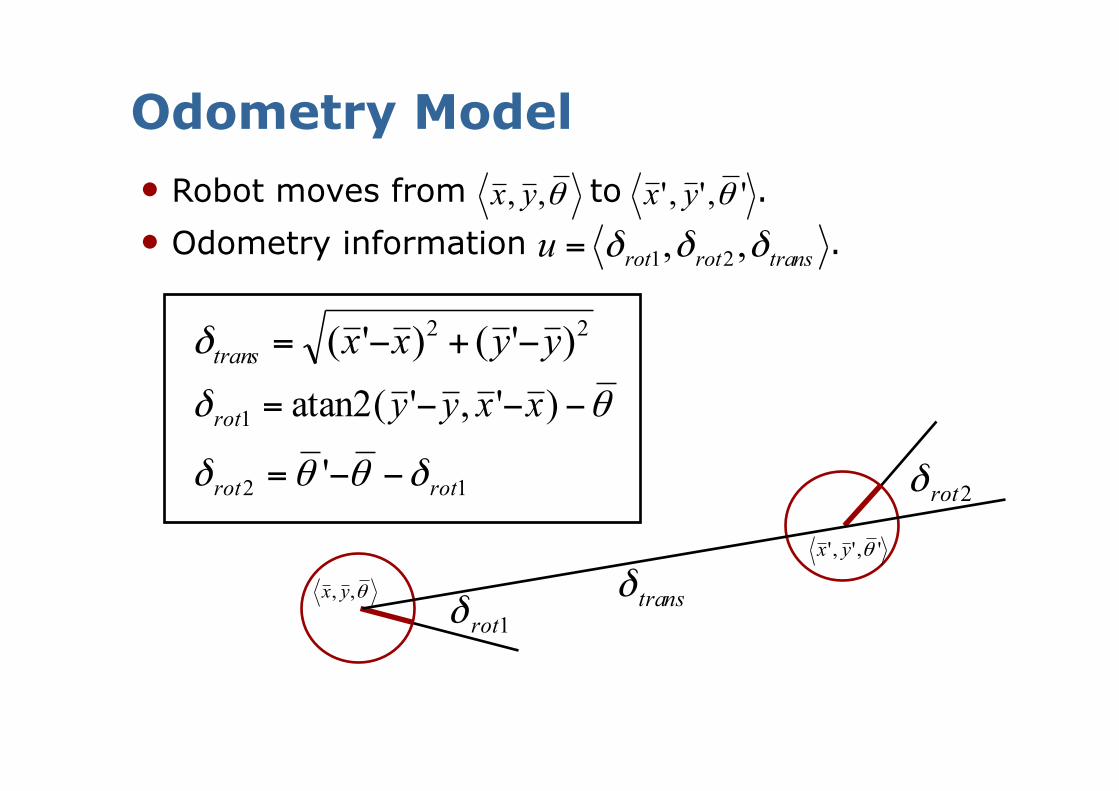
Odometry Model

22 )'()'( yyxxtrans −+−=δ

θδ −−−= )','(atan21 xxyyrot

12 ' rotrot δθθδ −−=

•  Robot moves from to . •  Odometry information .

θ,, yx ',',' θyx

transrotrotu δδδ ,, 21=

transδ1rotδ

2rotδ

θ,, yx

',',' θyx

11

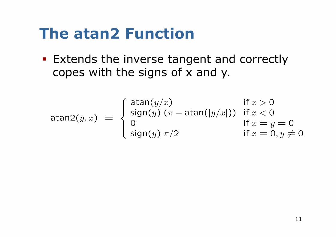
The atan2 Function §  Extends the inverse tangent and correctly

copes with the signs of x and y.

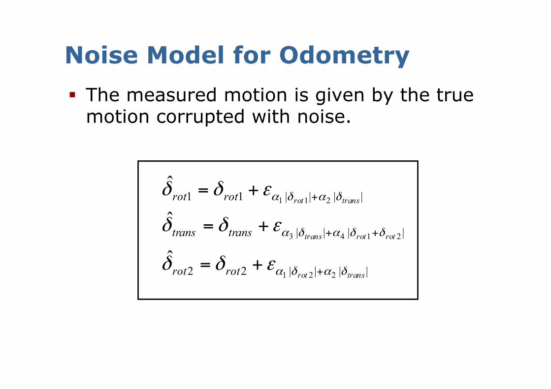
Noise Model for Odometry §  The measured motion is given by the true

motion corrupted with noise.

||||11 211ˆ

transrotrotrot δαδαεδδ ++=

||||22 221ˆ

transrotrotrot δαδαεδδ ++=

|||| 2143ˆ

rotrottranstranstrans δδαδαεδδ +++=

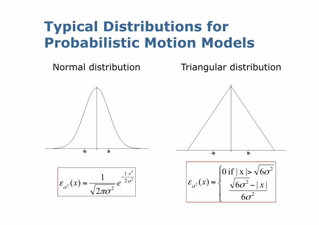
Typical Distributions for Probabilistic Motion Models

2

2

221

221)( σ

σ πσε

x

ex−

=⎪⎩

⎪⎨

⎧

−

>=

2

2

2

6||66|x|if0

)(2σ

σ

σεσ xx

Normal distribution Triangular distribution

14

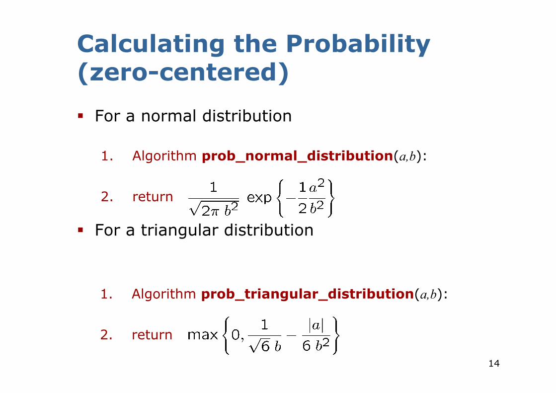
Calculating the Probability (zero-centered)

§  For a normal distribution

§  For a triangular distribution

1.  Algorithm prob_normal_distribution(a,b):

2.  return

1.  Algorithm prob_triangular_distribution(a,b):

2.  return

15

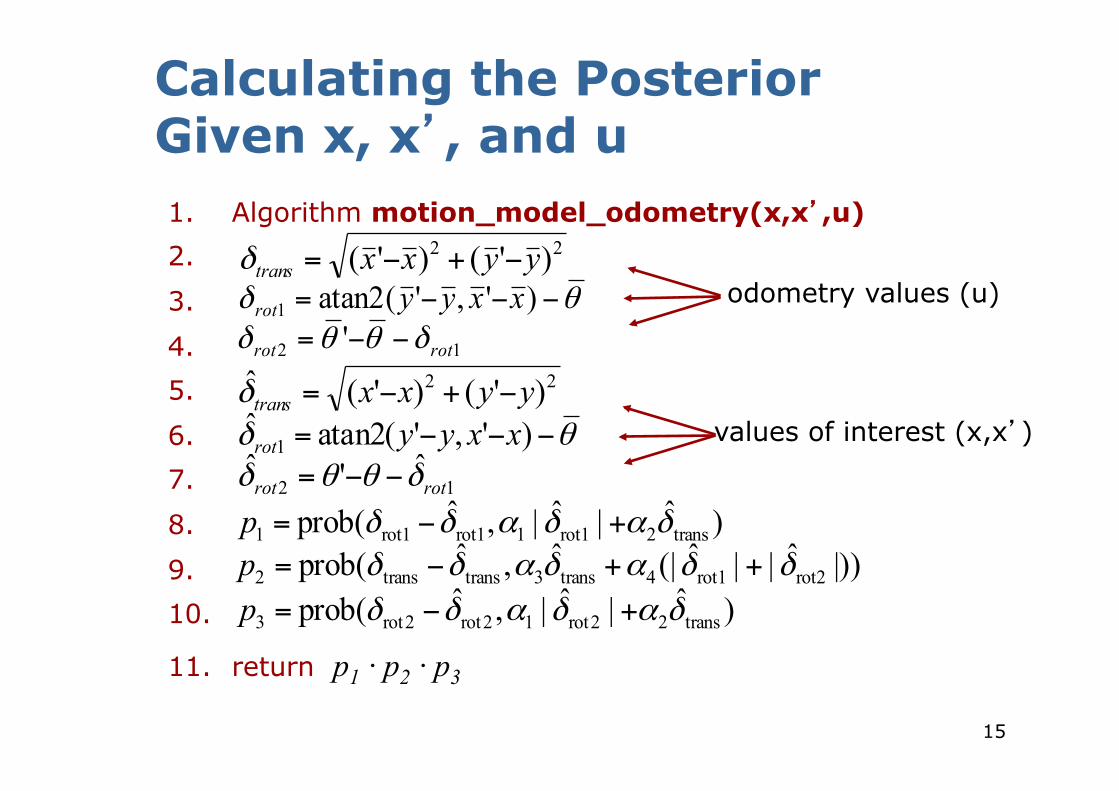
Calculating the Posterior Given x, x’, and u

22 )'()'( yyxxtrans −+−=δθδ −−−= )','(atan21 xxyyrot

12 ' rotrot δθθδ −−=22 )'()'(ˆ yyxxtrans −+−=δθδ −−−= )','(atan2ˆ

1 xxyyrot

12ˆ'ˆrotrot δθθδ −−=

)ˆ|ˆ|,ˆ(prob trans21rot11rot1rot1 δαδαδδ +−=p|))ˆ||ˆ(|ˆ,ˆ(prob rot2rot14trans3transtrans2 δδαδαδδ ++−=p

)ˆ|ˆ|,ˆ(prob trans22rot12rot2rot3 δαδαδδ +−=p

1.  Algorithm motion_model_odometry(x,x’,u) 2. 

3. 

4.  5. 

6.  7. 

8. 

9.  10. 

11.  return p1 · p2 · p3

odometry values (u)

values of interest (x,x’)

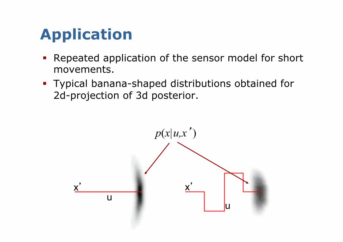
Application §  Repeated application of the sensor model for short

movements. §  Typical banana-shaped distributions obtained for

2d-projection of 3d posterior.

x’ u

p(x|u,x’)

u

x’

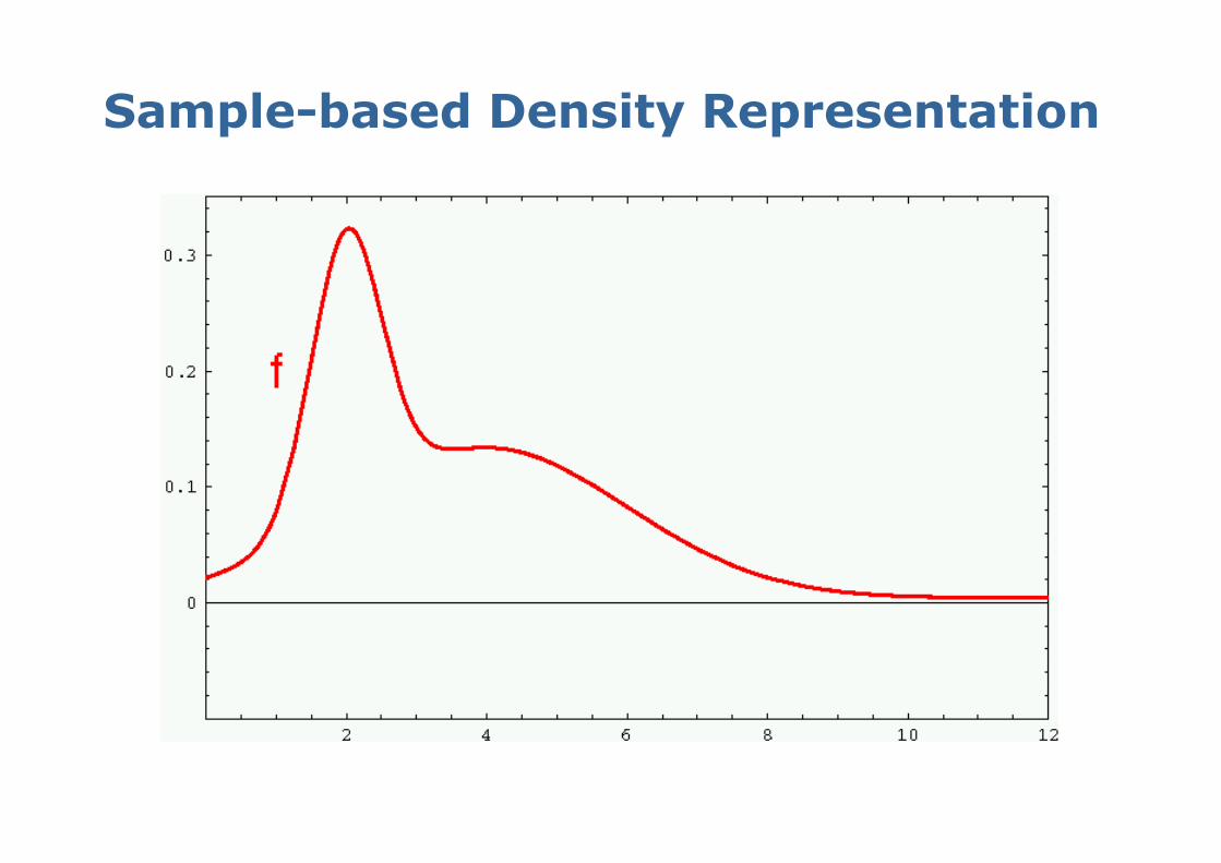
Sample-based Density Representation

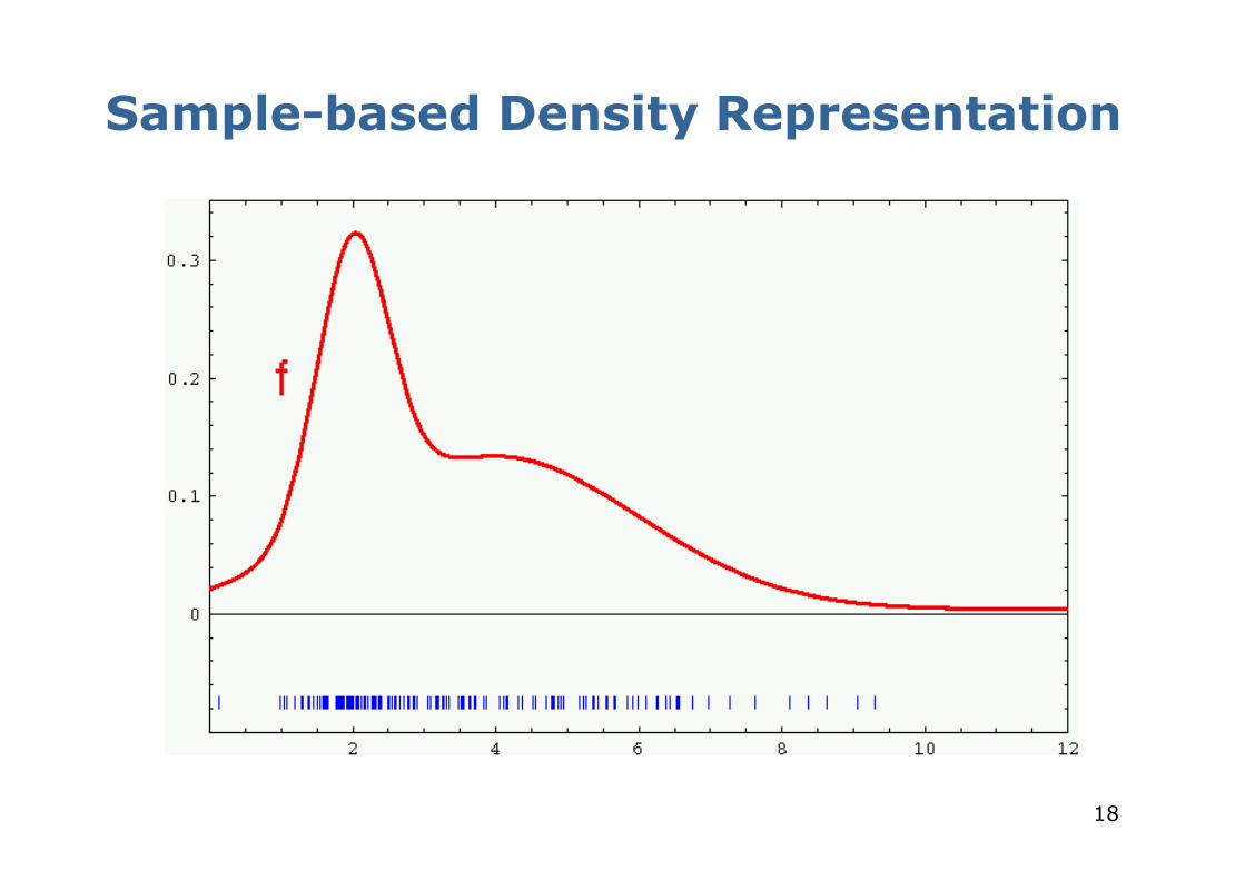
18

Sample-based Density Representation

19

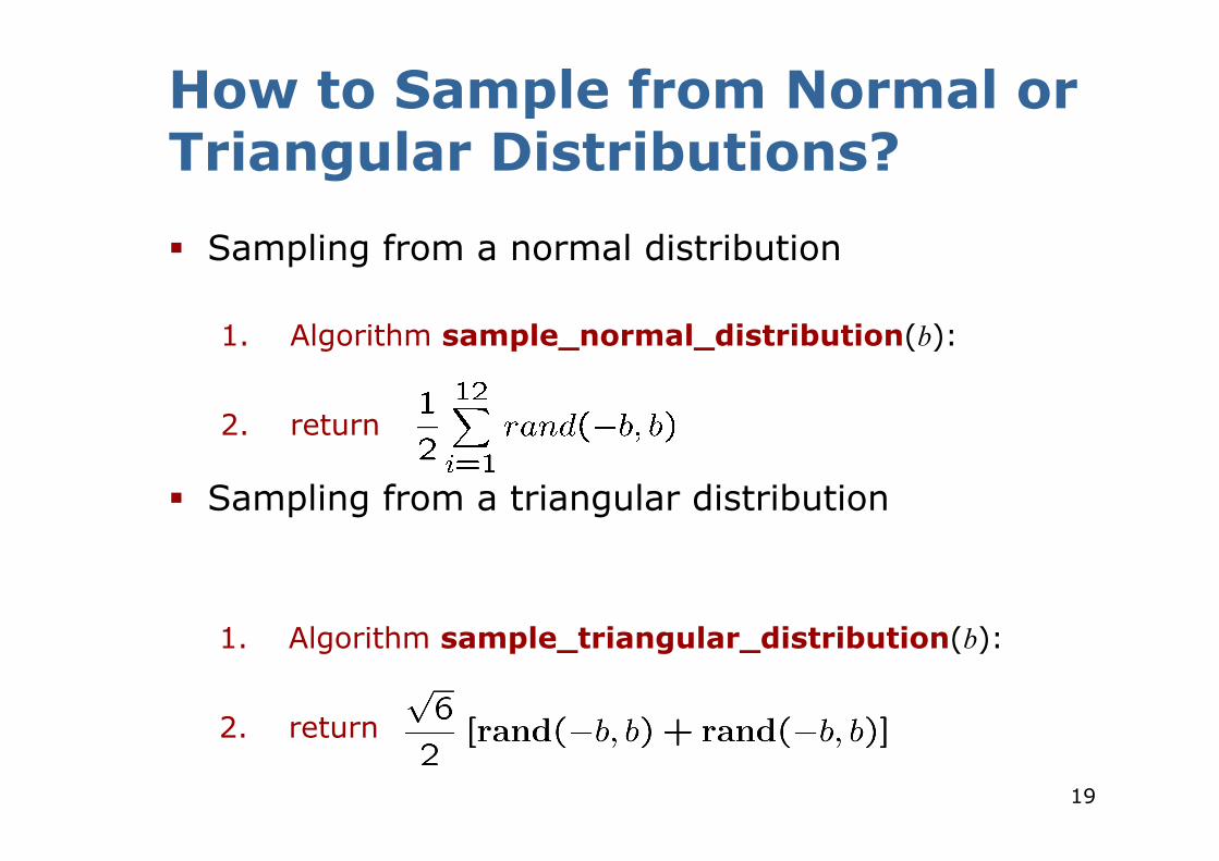
How to Sample from Normal or Triangular Distributions?

§  Sampling from a normal distribution

§  Sampling from a triangular distribution

1.  Algorithm sample_normal_distribution(b):

2.  return

1.  Algorithm sample_triangular_distribution(b):

2.  return

20

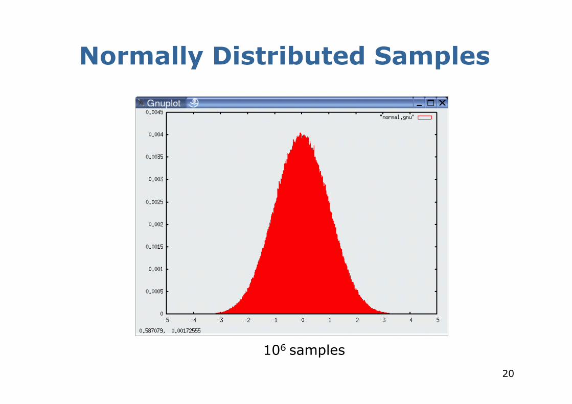
Normally Distributed Samples

106 samples

21

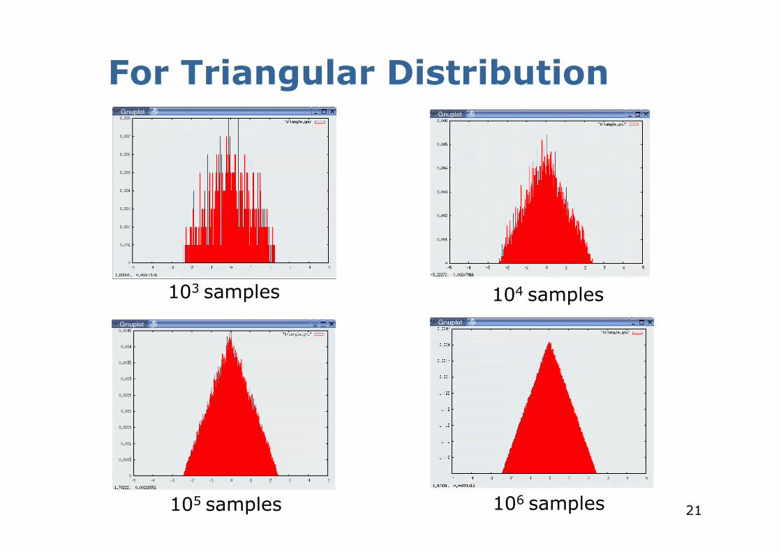
For Triangular Distribution

103 samples 104 samples

106 samples 105 samples

22

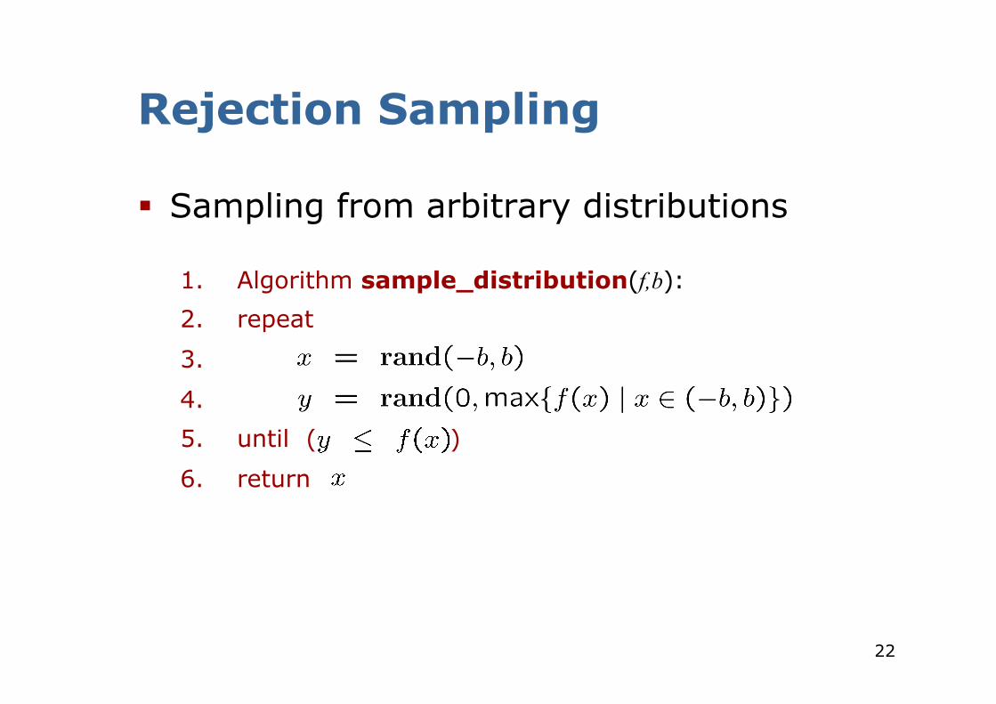
Rejection Sampling

§  Sampling from arbitrary distributions

1.  Algorithm sample_distribution(f,b): 2.  repeat

3. 

4.  5.  until ( )

6.  return

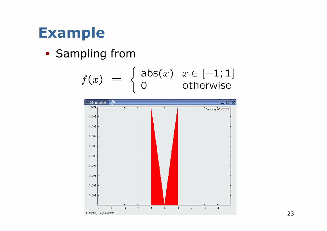
23

Example §  Sampling from

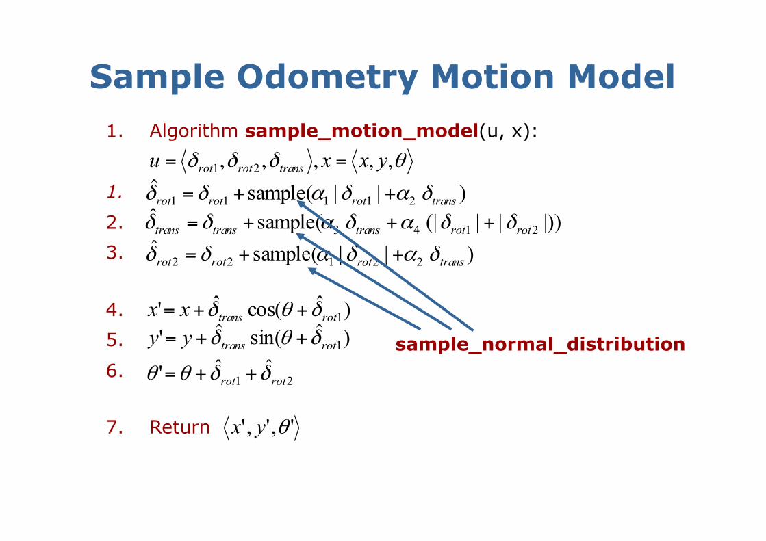
Sample Odometry Motion Model 1.  Algorithm sample_motion_model(u, x):

1. 

2.  3. 

4.  5. 

6. 

7.  Return

)||sample(ˆ21111 transrotrotrot δαδαδδ ++=

|))||(|sample(ˆ2143 rotrottranstranstrans δδαδαδδ +++=

)||sample(ˆ22122 transrotrotrot δαδαδδ ++=

)ˆcos(ˆ' 1rottransxx δθδ ++=)ˆsin(ˆ' 1rottransyy δθδ ++=

21ˆˆ' rotrot δδθθ ++=

',',' θyx

θδδδ ,,,,, 21 yxxu transrotrot ==

sample_normal_distribution

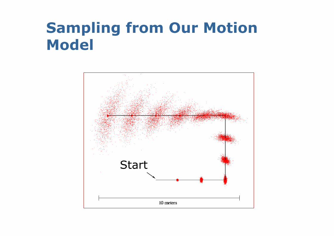
Sampling from Our Motion Model

Start

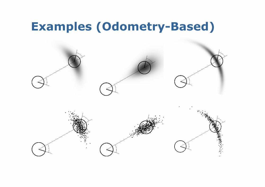
Examples (Odometry-Based)

27

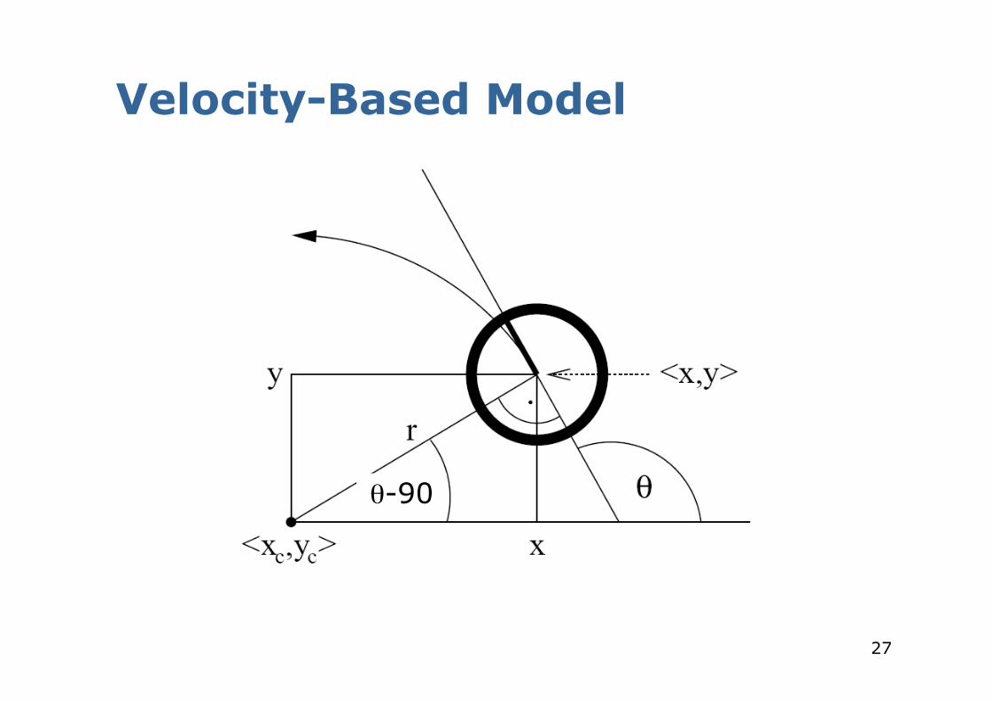
Velocity-Based Model

θ-90

28

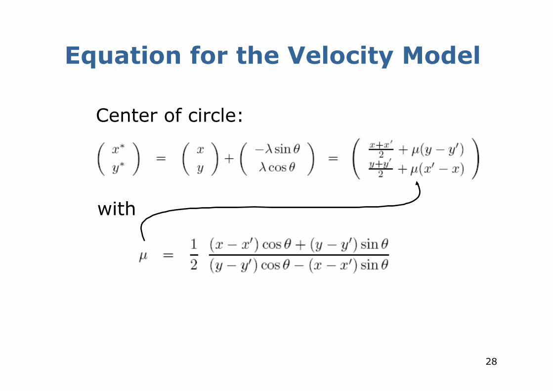
Equation for the Velocity Model

Center of circle:

with

29

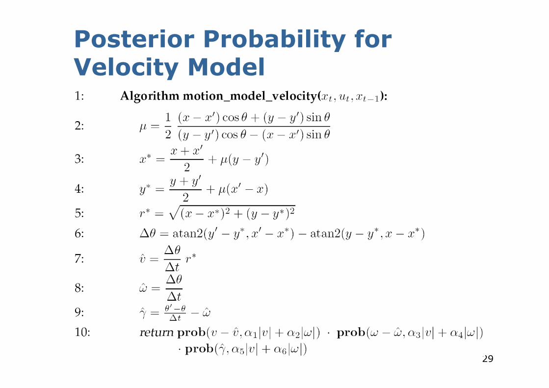
Posterior Probability for Velocity Model

30

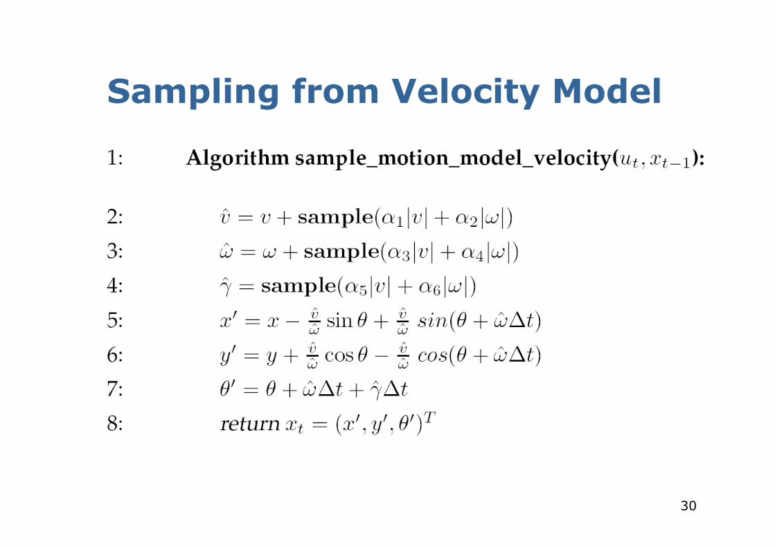
Sampling from Velocity Model

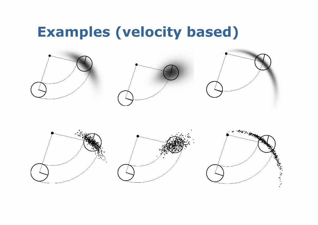
Examples (velocity based)

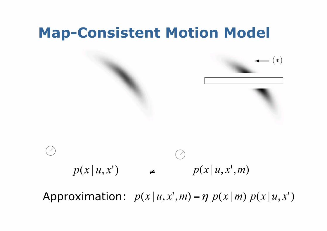
Map-Consistent Motion Model

)',|( xuxp ),',|( mxuxp≠

)',|()|(),',|( xuxpmxpmxuxp η=Approximation:

33

Summary §  We discussed motion models for odometry-based

and velocity-based systems §  We discussed ways to calculate the posterior

probability p(x| x’, u). §  We also described how to sample from p(x| x’, u). §  Typically the calculations are done in fixed time

intervals Δt. §  In practice, the parameters of the models have to

be learned. §  We also discussed an extended motion model that

takes the map into account.