Introduction to Matlab - University of Adelaide · Introduction to Matlab Matthew Roughan Applied...
114
Introduction to Matlab Matthew Roughan <[email protected]> Applied Mathematics, School of Mathematical Sciences The University of Adelaide April 11th, 2010
Transcript of Introduction to Matlab - University of Adelaide · Introduction to Matlab Matthew Roughan Applied...

Introduction to Matlab
Matthew Roughan<[email protected]>
Applied Mathematics, School of Mathematical SciencesThe University of Adelaide
April 11th, 2010

i
c© 2010 School of Mathematical SciencesThe University of AdelaideAll rights reserved

ii
Preface
These notes grew out of a set being used for a course called Scientific Computing. In that course,three programming languages were taught: Excel, MATLAB and C, with some emphasis on com-parison of the advantages, disadvantages, and commonalities between the three. This set of noteswas drawn from the MATLAB component of that course, as we often have a need to teach newstudents some elements of MATLAB , or to refresh their memory. However, as it was only onecomponent of a larger course, these notes are far from complete, and while they may comprise asuitable set for a student just starting MATLAB , there are plenty of other books and on-line refer-ence materials that are more substantial. Also, a reader maynotice comparisons with Excel or Cappearing at various places, due to the structure of the original course. Despite, this, these notesshould contain a reasonable introduction to programming (specifically programming for scientificor numerical purposes) in MATLAB .
Matthew Roughan

Contents
1 MATLAB Fundamentals 1
1.1 Reference books for MATLAB . . . . . . . . . . . . . . . . . . . . . . . . . . . 1
1.2 Getting started . . . . . . . . . . . . . . . . . . . . . . . . . . . . . . . . . .. . 2
1.3 How a program works . . . . . . . . . . . . . . . . . . . . . . . . . . . . . . . . 2
1.4 Variables . . . . . . . . . . . . . . . . . . . . . . . . . . . . . . . . . . . . . . 3
1.5 Script M-files . . . . . . . . . . . . . . . . . . . . . . . . . . . . . . . . . . . . 5
1.6 Useful features in the MATLAB window . . . . . . . . . . . . . . . . . . . . . . 6
1.7 Punctuation! . . . . . . . . . . . . . . . . . . . . . . . . . . . . . . . . . . . .. 7
1.8 Programming style . . . . . . . . . . . . . . . . . . . . . . . . . . . . . . . .. 7
2 Vectors and matrices 9
2.1 Initialising row vectors: explicit lists . . . . . . . . . . . .. . . . . . . . . . . . 9
2.2 Initialising row vectors: the colon operator : . . . . . . . .. . . . . . . . . . . . 10
2.3 Column vectors . . . . . . . . . . . . . . . . . . . . . . . . . . . . . . . . . . .10
2.4 Transposing vectors . . . . . . . . . . . . . . . . . . . . . . . . . . . . . .. . . 10
2.5 Concatenation . . . . . . . . . . . . . . . . . . . . . . . . . . . . . . . . . . .. 11
2.6 Subscripts . . . . . . . . . . . . . . . . . . . . . . . . . . . . . . . . . . . . . .11
2.7 Matrices . . . . . . . . . . . . . . . . . . . . . . . . . . . . . . . . . . . . . . . 12
2.8 MATLAB and matrices . . . . . . . . . . . . . . . . . . . . . . . . . . . . . . . 13
2.9 Solving linear equations with MATLAB . . . . . . . . . . . . . . . . . . . . . . 15
2.10 Strings . . . . . . . . . . . . . . . . . . . . . . . . . . . . . . . . . . . . . . . .16
2.11 Multi-dimensional arrays . . . . . . . . . . . . . . . . . . . . . . . .. . . . . . 17
3 MATLAB as a big calculator 19
3.1 Numbers . . . . . . . . . . . . . . . . . . . . . . . . . . . . . . . . . . . . . . . 19
3.2 Operators, expressions and statements . . . . . . . . . . . . . .. . . . . . . . . 20
iii

iv CONTENTS
3.3 Precedence of operators . . . . . . . . . . . . . . . . . . . . . . . . . . .. . . . 23
3.4 Vectorisation of formulae . . . . . . . . . . . . . . . . . . . . . . . . .. . . . . 24
4 Input/Output 27
4.1 disp . . . . . . . . . . . . . . . . . . . . . . . . . . . . . . . . . . . . . . . . 27
4.2 Theformat statement . . . . . . . . . . . . . . . . . . . . . . . . . . . . . . . 28
4.3 fprintf . . . . . . . . . . . . . . . . . . . . . . . . . . . . . . . . . . . . . . 28
4.4 Advanced I/O . . . . . . . . . . . . . . . . . . . . . . . . . . . . . . . . . . . . 32
5 Program flow control 35
5.1 Making decisions withif . . . . . . . . . . . . . . . . . . . . . . . . . . . . . 35
5.2 Repetition withfor . . . . . . . . . . . . . . . . . . . . . . . . . . . . . . . . 41
5.3 Non-deterministic repetition withwhile . . . . . . . . . . . . . . . . . . . . . 48
5.4 Programming style . . . . . . . . . . . . . . . . . . . . . . . . . . . . . . . .. 50
5.5 Other MATLAB statements . . . . . . . . . . . . . . . . . . . . . . . . . . . . . 51
6 Commonly used functions and variables 53
6.1 Constants . . . . . . . . . . . . . . . . . . . . . . . . . . . . . . . . . . . . . . 53
6.2 Elementary Mathematical Functions . . . . . . . . . . . . . . . . .. . . . . . . 54
6.3 Simple Vector/Matrix functions . . . . . . . . . . . . . . . . . . . .. . . . . . . 55
6.4 Set functions . . . . . . . . . . . . . . . . . . . . . . . . . . . . . . . . . . . .56
6.5 Test functions . . . . . . . . . . . . . . . . . . . . . . . . . . . . . . . . . . .. 56
6.6 String functions . . . . . . . . . . . . . . . . . . . . . . . . . . . . . . . . .. . 56
6.7 Dates and times . . . . . . . . . . . . . . . . . . . . . . . . . . . . . . . . . . .57
6.8 Utility functions . . . . . . . . . . . . . . . . . . . . . . . . . . . . . . . .. . . 57
6.9 More information . . . . . . . . . . . . . . . . . . . . . . . . . . . . . . . . .. 58
7 Graphics 59
7.1 Basic two-dimensional plots . . . . . . . . . . . . . . . . . . . . . . .. . . . . 59
7.2 Decorating the figure . . . . . . . . . . . . . . . . . . . . . . . . . . . . . .. . 59
7.3 Multiple plots . . . . . . . . . . . . . . . . . . . . . . . . . . . . . . . . . . .. 64
7.4 Printing graphs . . . . . . . . . . . . . . . . . . . . . . . . . . . . . . . . . .. 67
7.5 Colours . . . . . . . . . . . . . . . . . . . . . . . . . . . . . . . . . . . . . . . 68
7.6 Advanced two-dimensional plots . . . . . . . . . . . . . . . . . . . .. . . . . . 69
7.7 Three-dimensional plots . . . . . . . . . . . . . . . . . . . . . . . . . .. . . . 74

CONTENTS v
8 Defining Functions with M-files 79
8.1 Some examples . . . . . . . . . . . . . . . . . . . . . . . . . . . . . . . . . . . 79
8.2 The basic rules for function files . . . . . . . . . . . . . . . . . . . .. . . . . . 81
8.3 Function names as input variables withfeval . . . . . . . . . . . . . . . . . . 86
8.4 Inline and anonymous functions . . . . . . . . . . . . . . . . . . . . .. . . . . 87
8.5 Recursion . . . . . . . . . . . . . . . . . . . . . . . . . . . . . . . . . . . . . . 87
9 0-1 vectors 93
9.1 Combining logical and numerical vectors . . . . . . . . . . . . .. . . . . . . . 94
9.2 Additional tests . . . . . . . . . . . . . . . . . . . . . . . . . . . . . . . . .. . 98
9.3 Thefind function . . . . . . . . . . . . . . . . . . . . . . . . . . . . . . . . . 98
10 The Optimization Toolbox 101
10.1 Linear Programming . . . . . . . . . . . . . . . . . . . . . . . . . . . . . .. . 101
10.2 Why use MATLAB for optimization . . . . . . . . . . . . . . . . . . . . . . . . 103
11 MATLAB Roundup 105
11.1 More stuff . . . . . . . . . . . . . . . . . . . . . . . . . . . . . . . . . . . . . .105
11.2 Limitations . . . . . . . . . . . . . . . . . . . . . . . . . . . . . . . . . . . .. 105
11.3 Summary . . . . . . . . . . . . . . . . . . . . . . . . . . . . . . . . . . . . . . 106

vi CONTENTS
Chapter 1
MATLAB Fundamentals
We can characterise MATLAB as follows. It is
• Imperative: we tell the computer what to do.
• Procedural: a program is written as a series of tasks (procedures) to do ina specified order.
• High-level: MATLAB is written in a high-level programming language which resembles amixture of English and mathematics. The exact form has to differ from both because it needsto be more precise than English (computer are fast but stupid), and because a typewriterkeyboard (which we will use for entering programs) has limited keys.
• Interpreted: MATLAB uses an interpreter to translate our high-level commands into some-thing the machine can do. It does the translation (almost) onthe spot when we type a com-mand. A MATLAB interpreter exists for most common computing environments, includingWindows, MacOS, and Linux, so MATLAB code is very portable (if it is written carefully).
1.1 Reference books forMATLAB
This course draws from the following text which is availablein the Reserve section of the BarrSmith library.
1. Hahn, B.D.EssentialMATLAB for Scientists and engineers(Arnold, London) 1997/2002/2007.
The 1997 version relates to MATLAB 4, 2002 to MATLAB 6.1 and 2007 to MATLAB 7.2. OurLabs now use MATLAB version 7. However, most of this course is not dependent on the versionof MATLAB used.
Matlab has extensive built in help, either through typinghelp followed by a topic or func-tion, or through the MATLAB menus. There is also extensive on-line help on the Internet,via theMathworks web page, or other 3rd party tutorials.
The Uni book shop can order in a student version of MATLAB for less than $200, but you donot need this to complete the course. There is also a free program very similar to MATLAB called
1

2 CHAPTER 1. MATLAB FUNDAMENTALS
octave , but it does have some differences particularly in the user interface, and so we do notrecommend it for this course, though you may wish to use it in the future.
1.2 Getting started
Invokingmatlab produces a MATLAB window similar to Figure 1.1.
Figure 1.1: Matlab window
The>> is the MATLAB prompt. Initially you will enter commands at this prompt butlater wewill see how to write and use. m files using a text editor.
For an overview of the help facility typehelp help . For a menu-driven graphical userinterface of the help facility, typehelpwin , or use the HELP menu. For help with a specificcommand typehelp command name wherecommand name is the name of the commandwith which you seek help.
To exit MATLAB typequit or use the FILE menu.
1.3 How a program works
Consider the following piece of MATLAB code, which we might type at the MATLAB prompt.

1.4. VARIABLES 3
balance = 1000;rate = 0.09;interest = rate * balance;balance = balance + interest;disp( ’New balance:’ )disp( balance )
Typing this in the MATLAB command window we get the following output:
New balance:1090
The statements in our program are interpreted by MATLAB as
1. assign the value 1000 to the variablebalance .
2. assign the value 0.09 to the variablerate .
3. multiply the value ofrate by the value ofbalance and assign the answer tointerest .
4. display (in the command window) the message given in single quotes.
5. display the value ofbalance .
MATLAB processes the statements inorder from the top down. When the program finishes thevariables used will have the values
balance: 1090interest: 90rate: 0.09
1.4 Variables
A variable is a programming structure we define to hold a value. It is called a variable because wecan change the value it holds. A variable is created by assigning a value to it. For example
a=98
Any operations that assign a value to a variable automatically create the variable if needed, oroverwrites its current value if it already exists. If the right-hand side of an assignment operationrefers to a non-existent variable you will get the error message
Undefined function or variable
MATLAB allows us to give a variable a value of a string, number, orarray (a synonym for a vectoror matrix). In fact, by default all variables are arrays. Scalars are just stored as1 × 1 arrays.
4 CHAPTER 1. MATLAB FUNDAMENTALS
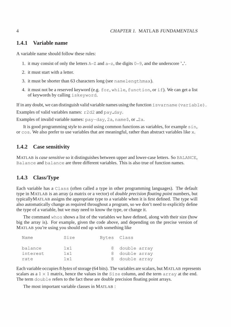
1.4.1 Variable name
A variable name should follow these rules:
1. it may consist of only the lettersA–Z anda–z , the digits0–9, and the underscore ’’.
2. it must start with a letter.
3. it must be shorter than 63 characters long (seenamelengthmax ).
4. it must not be a reserved keyword (e.g.for , while , function , or if ). We can get a listof keywords by callingiskeyword .
If in any doubt, we can distinguish valid variable names using the functionisvarname( variable) .
Examples of valid variables names:r2d2 andpay day .
Examples of invalid variable names:pay-day , 2a , name$, or 2a .
It is good programming style to avoid using common functionsas variables, for examplesin ,or cos . We also prefer to use variables that are meaningful, ratherthan abstract variables likex .
1.4.2 Case sensitivity
MATLAB is case sensitiveso it distinguishes between upper and lower-case letters. So BALANCE,Balance andbalance are three different variables. This is also true of functionnames.
1.4.3 Class/Type
Each variable has aClass (often called a type in other programming languages). The defaulttype in MATLAB is an array (a matrix or a vector) ofdouble precision floating pointnumbers, buttypicallyMATLAB assigns the appropriate type to a variable when it is first defined. The type willalso automatically change as required throughout a program, so we don’t need to explicitly definethe type of a variable, but we may need to know the type, or change it.
The commandwhos shows a list of the variables we have defined, along with theirsize (howbig the array is). For example, given the code above, and depending on the precise version ofMATLAB you’re using you should end up with something like
Name Size Bytes Class
balance 1x1 8 double arrayinterest 1x1 8 double arrayrate 1x1 8 double array
Each variable occupies 8bytesof storage (64 bits). The variables are scalars, but MATLAB representsscalars as a1 × 1 matrix, hence the values in theSize column, and the termarray at the end.The termdouble refers to the fact these are double precision floating point arrays.
The most important variable classes in MATLAB :

1.5. SCRIPT M-FILES 5
• double precision floating point: numbers are the default way of representing real numbers.Eachdouble uses 8 bytes or memory. MATLAB uses the IEEE Standard 754 for its floatingpoint representation.
• logical: or Boolean variables represent the values TRUE and FALSE, using 1 and 0 respec-tively. We can define a logical variable using logical operators like==. In principle a logicalvariable needs only 1 bit, but MATLAB stores each in 1 byte.
• char: represents a ASCII tex character, i.e., the typical typewriter letters. An array of theseforms a string (a piece of text). We can define a string using single quotes, e.g.
the_string = ’Hello, world!’;
Quotes may be included in a string by repeating them twice.the_string = ’Hello, ’’world’’!’;
There are other types in MATLAB , e.g. single , int8 , uint16 , function_handle , etc.,but these are less commonly used. Also, one of the pleasures of programming in MATLAB is thatone typically doesn’t have to worry about the type of a variable as MATLAB handles these foryou, unless you have a specific requirement. There are also more advanced data types such ascell andstruct that are outside the scope of this course. MATLAB also allows more objectoriented classes such as<class_name> , again outside the scope of this course.help classcan provide more details.
In MATLAB we can often ignore a variable’s class and allow MATLAB to work out the detailsfor us, but there are some issues you need to be aware of.
• Double-precision floating point numbers try to represent a real number, but they do NOT dothis to arbitrary precision. This allows numerical errors in calculations, and if one does notprogram carefully these can become a problem, The classic mistake is to test whether twofloating points numbers are equal by writing, for instancex == y . This may fail becausethe two numbers are very slightly different. For instance, in MATLAB sin(π) 6= 0, becauseMATLAB only stores an approximate value ofπ. We will later see how to do this correctly.
• Strings are not a “scalar” variable, but rather are represented as an array of characters. Thisis sometimes important when operating on them.
1.5 Script M-files
A M ATLAB program saved from a text editor with the.m extension is called ascript file. As anexample, let’s save our earlier interest program in a file with the namecalc interest.m .
balance = 1000;rate = 0.09;interest = rate * balance;balance = balance + interest;disp( ’New balance:’ )disp( balance )

6 CHAPTER 1. MATLAB FUNDAMENTALS
To run the programcalc interest we simply enter the name
calc_interest
at the MATLAB prompt, and each command in the file will be executed in order.A script file maybe listed in the command window with the commandtype , e.g.
type calc_interest
and MATLAB would output the above.m file.
MATLAB has a built in editor that we can use via the MATLAB menus. Go to FILE-> NEW tocreate a new.m file, or FILE-> OPEN to edit an existing file. The editor has many useful features,e.g. it highlights different parts of the code in different colours to help identify, e.g. comments. Itputs line numbers next to the lines of code to aid in debugging, and it has built in debugging tools.Other text editors also support some or all of these features, but for the purposes of this course wewill use MATLAB ’s built in editor.
1.6 Useful features in theMATLAB window
The MATLAB window has some useful features. On the left-hand (by default) side the windowhas sections allowing us to display the current Workspace, the current directory, and the commandhistory.
1.6.1 The Directory
One of the options we can display is the current directory (sometimes called a folder), showing alist of the.m files we have created. We can also manage this directory, or change directories.
1.6.2 The Workspace
A fundamental concept in MATLAB is theworkspace. If we enter the commandwho we shouldsee a list of variables, for instance, given the previous examplewho would return
Your variables are:
balance interest rate
We can also see the workspace in the top left frame of the MATLAB window.
All variables you create during a session remain in the workspace until youclear them,either individually, or ifclear is called by itself it clears the whole workspace.
The MATLAB window can also display a graphic of the workspace, showing alist of variablestheir size, and a graphic representation of what type of variable they are.

1.7. PUNCTUATION! 7
1.6.3 Command history
The history contains a list of all of the commands we type. It is convenient for us to be able toreview this, but more importantly, we can repeat a command easily. The up-arrow on the keyboardallows us to scroll back through these past commands. We can filter the command list by typing afew letters at the command prompt and then using the up-arrow. MATLAB will then scroll throughcommands that match the letters we typed. This can save us a lot of typing.
1.7 Punctuation!
By default, MATLAB has one command per line. When you hit the enter or return key to start anew line, MATLAB interprets the current command. In a.m file, we usually have one commandper line of the file. So a single line is like a “sentence” in English, but we don’t need to put a fullstop at the end.
In MATLAB , various symbols can alter this behaviour.
• , We can put more than one command on a line with a comma, e.g.x=1, y=x
The commands are executed in order from left to right.
• ... If we have a complicated formula that won’t easily fit on one line, we can spread itover two lines using three full stops, e.g.,
x = (1 + 2 + 3 + 4 + 5 ...+ 6 + 7)
• % The percentage sign is use to denote acomment. Comments are text in the programthat has no effect on the program itself. In MATLAB , everything on a line that appears afterthe % sign is ignored. Comments are very useful for making code easier to understand, e.g.,
g = 9.8 % the gravitational constant in m/sˆ2
• ; By default, when we enter a MATLAB command, the result of that command willappear in the command window. If we wish to suppress this behaviour we end the line witha semi-colon “;”, and the command will execute silently. Omitting the semi-colons can saveus typingdisp , so we only really usedisp for teaching purposes.
1.8 Programming style
It is extremely important for you to develop the art of writing programs which are laid out well andwith all the logic described clearly. Good comments are not fun to write, and are often omitted,or done carelessly. However, good comments make a program more easily maintainable, andreusable. Failing to comment code may seem to save time, but generally costs companies a greatdeal more than it saves.
In programming MATLAB we expect you to

8 CHAPTER 1. MATLAB FUNDAMENTALS
• Put a comment at the start of all .m files explaining what the file does, who wrote it andwhen, and some details of any inputs, outputs, or other assumptions. It should also list howit relates to any other programs. Often it is useful to provide a reference to the source of analgorithm, or a set of data.
• Variable names should be meaningful. For exampleinterest_rate is preferable tox .Where possible, match variable names to the reference text.
• Variable names should not overlap common functions.
• Even where variable names are chosen well, it is useful to accompany a variable definitionwith a comment. Sometimes this can help understand details of the variable (for instance,we might have two interest rates in our program and wish to help a reader understand whichis which). Another use for comments is to specify units, e.g.
g = 9.8 % the gravitational constant in m/sˆ2
• Comments can be otherwise used to highlight key steps in an algorithm, or otherwise clarifycode.
• Spaces can be used in expressions to make them easily readable, e.g. on either side of theequal signs as inx = [1,2,3] . We can also use brackets to make complex expressionseasier to understand.
• Blank lines can be used to separate different parts of the program. Another convention is touse a row of % signs to separate major segments of code.
• Don’t “hardwire” values. Where-ever you have a value that you use more than once ina program, you should assign that value to a variable, and usethe variable. This makesmaintenance much easier as you will only have to change the value in one place to updatethe program.
You may want to develop your own style but it is important to pay attention to readability. A goodapproach is to imagine another person who has to read your code, and modify it. Then apply theprinciple “Do unto others as you would have done to you.” Do the things that you would appreciatewhen you are reading other peoples’ code.
Perhaps a more compelling maxim comes in the form of a quote from Damien Conway (PerlBest Practices)
Always code as if the guy who ends up maintaining your code will be a violent psy-chopath who knows where you live.
Chapter 2
Vectors and matrices
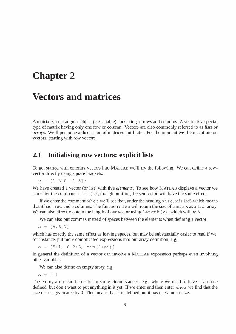
A matrix is a rectangular object (e.g. a table) consisting ofrows and columns. A vector is a specialtype of matrix having only one row or column. Vectors are alsocommonly referred to aslists orarrays. We’ll postpone a discussion of matrices until later. For the moment we’ll concentrate onvectors, starting withrow vectors.
2.1 Initialising row vectors: explicit lists
To get started with entering vectors into MATLAB we’ll try the following. We can define a row-vector directly using square brackets.
x = [1 3 0 -1 5];
We have created a vector (or list) with fiveelements. To see how MATLAB displays a vector wecan enter the commanddisp(x) , though omitting the semicolon will have the same effect.
If we enter the commandwhos we’ll see that, under the headingsize , x is 1x5 which meansthat it has 1 row and 5 columns. The functionsize will return the size of a matrix as a1x5 array.We can also directly obtain the length of our vector usinglength(x) , which will be 5.
We can also put commas instead of spaces between the elementswhen defining a vector
a = [5,6,7]
which has exactly the same effect as leaving spaces, but may be substantially easier to read if we,for instance, put more complicated expressions into our array definition, e.g,
a = [5+1, 6-2 * 3, sin(2 * pi)]
In general the definition of a vector can involve a MATLAB expression perhaps even involvingother variables.
We can also define an empty array, e.g.
x = [ ]
The empty array can be useful in some circumstances, e.g., where we need to have a variabledefined, but don’t want to put anything in it yet. If we enter and then enterwhos we find that thesize ofx is given as 0 by 0. This means thatx is defined but it has no value or size.
9

10 CHAPTER 2. VECTORS AND MATRICES
2.2 Initialising row vectors: the colon operator :
A vector can also be generated with thecolon operator. If we enter the following:x = 1:10
we obtain a vector with elements that are the integers (1,2,3,4,5,6,7,8,9,10). The commandx = 1:0.5:4
produces a vector with the elements (1, 1.5, 2, 2.5, 3, 3.5, 4)each of which increases in incrementsof 0.5. The colons separate three values, and themiddlevalue is the increment. Similarly
x = 10:-1:1
produces a vector with elements (10,9,8,7,6,5,4,3,2,1) since the increment is negative. Anotherexample is
x = 1:2:6
In this case the elements are 1,3,5. Note that when the increment is positive but not equal to 1 thelast element is not allowed to exceed the value after the second colon.
2.3 Column vectors
We can create a column vector by reusing the semi-colon (thisis a different use from when we enda line with a semi-colon). We simple define a column vector by
x = [ 1; 2; 3 ]
which defines the 3x1 column vector
x =
123
2.4 Transposing vectors
We can transpose between row and column vectors using the a single quote, orapostrophe’ , e.g.,when we enter
y = [1 4 8]’
we get the column vector
y =
148
with 3 rows and 1 column. Likewise,y = [4; 5; 1]’
Results iny = (4, 5, 1).
[Warning: actually this operation gives the conjugate transpose. Replace 1 by i in this exampleand inspect the output. For simple transpose use.’ rather than a simple apostrophe. ]

2.5. CONCATENATION 11
2.5 Concatenation
Concatenation basically means sticking one array on the endof another. We can concatenate twovectors by placing them within square brackets, e.g. if we take
a = [1 2 3]b = [4 5]c = [a -b]
Thenc = (1, 2, 3, 4, 5). Or for column vectorsa = [1; 2]b = [4; 5]c = [a; -b]
Then
c =
1245
2.6 Subscripts
We can refer to particular elements of a vector by means ofsubscripts.
1. Set up the vectorr = [2 4 8 16 32 64 128]
2. The commandr(3)
gives the third element of the vectorr (the value is 8). The number 3 is thesubscript.
3. The commandr(2:4)
will give thesecond, third andfourthelements of the vectorr , i.e., the vector(4, 8, 16).
4. The commandr(1:2:7)
returns the odd terms(2, 8, 32, 128).
5. We can use an empty vector toremoveelements from a vector. The commandr([1 7 2]) = [ ]
will remove the elements 1,7 and 2, so nowr will look like
r = (8, 16, 32, 64).
6. There is a special termend we can use to mean the last element of an array, e.g. ifr = [2 4 8 16 32 64 128]
Thenr(5:end) would be the array(32, 64, 128).
Warning: MATLAB subscripts start at 1 (the integer 1 means the 1st element of the array).In C, subscripts start at 0. This is a very common source of errors for people who have towrite code in both.

12 CHAPTER 2. VECTORS AND MATRICES
2.7 Matrices
A matrix may be thought of as a table consisting of rows and columns. We enter a matrix just aswe did for a vector, using a semi-colon to indicate the end of arow. The statement
a = [1 2 3 ; 4 5 6]results in
a =1 2 34 5 6
A matrix may be transposed in the same way as for a vector. An apostrophe will interchangingrows and columns, e.g., the statementa’ results in
ans =1 42 53 6
A matrix can also be constructed from column vectors of the same length by concatenation. Thestatements
x = 0:30:180table = [x’ sin(x * pi/180)’]
concatenates the two column vectorsx andsin(x * pi/180)’ together into a7x7 matrixtable =
0 030.0000 0.500060.0000 0.886090.0000 1.0000
120.0000 0.8660150.0000 0.5000180.0000 0.0000
Subscripts work as expected. The element in theith row, andjth column, i.e., the(i, j)thelement of matrixA can be accessed usingA(i,j) . As before we can use vector subscripts toextract a portion of the matrix. For instance
table([1 2 3], 2)
ans =0
0.50000.8660
We can replace the whole possible range of an index using either 1:end , or even more simplyjust : . For instance
table([1 2 3], :)
ans =0 0
30.0000 0.500060.0000 0.8660

2.8. MATLAB AND MATRICES 13
2.8 MATLAB and matrices
One of the most powerful features of MATLAB is its ability to operate directly on matrices. Forinstance, we can multiply all of the elements of a matrix by a scalar simply using the standardmultiplication operator∗. In the above example the functionsin acts on each element of thecolumn vector, returning a column vector whose elements aresine of x . We will discuss thisfurther in the following chapter, but some simple examples are
A = [1; 2; 3];b = 3;x = b * A;y = b + A;
which will result in
x =
369
y =
456
There are also special operators defined in MATLAB for performing matrix operators. A simpleexample isx = [1, 2, 3].ˆ2 , where the.ˆ operator squares each element of the vectorgiving x = (1, 4, 9). A more sophisticated example is given below.
Example: If a stone is thrown vertically upward with an initial speedu, its vertical displacements after timet has elapsed is given by the formula
s = ut − 1
2gt2,
whereg is the acceleration due to gravity. Air resistance has been ignored. We would like tocompute the value ofs over a period of about13sec at intervals of0.1 seconds and to plot thedistance-time graph over this period. Our plan for this problem is as follows:
1. Get the data (g, u andt) into MATLAB .
2. Calculate the value ofs according to the formula.
3. Plot the graph ofs againstt.
The resulting program is
% Vertical motion under the action of gravityg = 9.8; % acceleration due to gravityu = 60; % initial velocity (metres/sec)t = 0 : 0.1 : 13 ; % the time in secondss = u * t - g/2 * t.ˆ2 ; % vertical displacement in metres
plot(t, s)title( ’Vertical motion under gravity’)xlabel( ’Time’ ) , ylabel( ’Vertical displacement’ )grid

14 CHAPTER 2. VECTORS AND MATRICES
0 2 4 6 8 10 12 14-50
0
50
100
150
200Vertical motion under gravity
Time
Ver
tical
dis
plac
emen
t
Figure 2.1: Vertical motion under gravity
The graphical output is shown in figure 2.1.
An additional constructor that is often useful when building matrices is themeshgrid func-tion. It works as follows: take two vectorsx andy , of lengthsN andM respectively, and
[X, Y] = meshgrid(x, y);
will result in X andY that areN × M matrices, with the rows ofX the vectorx , and the columnsof Y are the vectorsy . Remember that MATLAB variables are case sensitive soX is a differentvariable tox .
A simple example is the construction of a multiplication table much as we did in Excel. Usethe following commands
x = 1:12;y = 1:12;[X, Y] = meshgrid(x, y);Table = X . * Y;
Now the variableTable will contain the multiplication table.

2.9. SOLVING LINEAR EQUATIONS WITHMATLAB 15
2.9 Solving linear equations withMATLAB
One of the most common uses for matrices is in solving a set of linear equations, e.g., we havethree variablesx1, x2, andx3 and three equations
3x1 + 2x2 + x3 = 2, (2.1)
x1 + x2 + 3x3 = 2, (2.2)
2x1 − x2 + 2x3 = 1. (2.3)
We can represent a set of such equations by
Ax = b,
where
A =
3 2 11 1 32 −1 2
, x =
x1
x2
x3
and b =
221
In MATLAB we can solve a set of equations such as this simply using
x = A \ b
WhenA is invertible, this is equivalent tox = A−1b computed using Gaussian elimination. We
can obtain the inverse ofA directly using
inv(A)
Note that whenA is not invertible, or non-square MATLAB ’s behaviour is more complex. Also,it is possible to have unexpected results if a matrix isill conditioned, e.g.,
A = [2 eps -eps; eps 1 1; -eps 1 1];b = [2; eps + 2; -eps + 2];x = A \ b
MATLAB will print a warning in this case saying
Warning: Matrix is close to singular or badly scaled.Results may be inaccurate. RCOND = 2.465190e-32.
We can obtain more information usinghelp mldivide .

16 CHAPTER 2. VECTORS AND MATRICES
2.10 Strings
Text can be stored in variables in MATLAB , and the result is usually called astring.The standardway to create and assign a string to a variable is use single quotes, e.g.,
the_string = ’Hello, world!’;
Quotes may be included in a string by repeating them twice.
the_string = ’Hello, ’’world’’!’;
In the latter case,whos will tell us that the_string is a 1x15 array of characters taking 30bytes.
Actually, a MATLAB string is an array of numbers, each storing the “Unicode” number for acharacter in the string. Unicode consists of a repertoire ofabout 100,000 characters from mostworld languages. The most commonly used encodings (in English) are ASCII characters. We canwrite out a table of the printable ASCII characters,
ascii = [char(32:79); char(80:127)]ascii =
!"#$%&’() * +,-./0123456789:;<=>?@ABCDEFGHIJKLMNOPQRSTUVWXYZ[\]ˆ_‘abcdefghijklmnopqrstuvwxyz{|}˜ˆ
For more information about ASCII see, for example,http://en.wikipedia.org/wiki/ASCII . MATLAB stores the a numeric code associated with each character, sooperations suchasthe_string+1 will have unexpected results (it shifts us down the alphabetby one). We canconvert between a character array, and an array of double precision numbers using the conversionfunctionschar() anddouble() .
A string is an array, and hence they may be concatenated just as other arrays, e.g.,
the_string = [’Hello, ’ ’world!’];
A typical string is just a row vector of characters, but we canform matrices of characters. Therecan be problems, however, with such matrices. For instance,it is often appealing to interpret themas a series of lines of text. In contrast to typical text, these are held in an array, and so each rowmust be the same length. Also operations on these arrays (e.g. transpose) often have unexpectedresults, so care must be taken. What is often needed is an actual array of strings, which can beformed in MATLAB using acell array, but such arrays fall outside the scope of this course.

2.11. MULTI-DIMENSIONAL ARRAYS 17
2.11 Multi-dimensional arrays
MATLAB allows one to construct multi-dimensional arrays. Often this is simplest using standardconstructors of matrices, such asones , zeros , andrand , which allow for more than 2 inputparameters with a resulting multi-dimensional matrix, e.g.,
A = ones(3,2,4);
will return a 3 × 2 × 4 array. We can access its elements using, for instance,A(i,j,k) , andsize(A) will return the vector[3 2 4] . DisplayingA with thedisp function will return
(:,:,1) =1 11 11 1
(:,:,2) =1 11 11 1
(:,:,3) =1 11 11 1
(:,:,4) =1 11 11 1
where each group specifies a3 × 2 subarray, or which there are four.

18 CHAPTER 2. VECTORS AND MATRICES

Chapter 3
MATLAB as a big calculator
One of the key features of MATLAB is the ability to do complicated calculations. In some ways itresembles a great big calculator, but its capabilities, andeven the rules for how calculations workare rather different from your standard calculator.
3.1 Numbers
3.1.1 Writing numbers
Numbers can be represented in MATLAB in the usual decimal form, e.g.
1.2345 , -123 , .00001
A number may also be represented inscientific notation, e.g.1.2345 × 106 = 1, 234, 500 may berepresented in MATLAB as
1.2345e6
3.1.2 Numerical errors
As noted above, numbers are stored as double precision floating point variables, but this meansthere will be small errors in some numbers. For instance, irrational numbers such as as1/3, π, or√
2 are not possible to represent exactly, but you may find errorseven in numbers that are exact,e.g.1.1010101010101010101 will be stored as approximately1.1010101010101009944. Note thatwhen you use thedisp() function, you only see the value output to a fixed precision.
The function/variableeps tells us something about the spacing between floating point num-bers. Used as a variable in the current version of MATLAB , eps = 2.220446049250313e-16 ,which gives us difference between1 and the next largest number that can be represented inMATLAB , but used as a function it can tells us a great deal more. Usehelp eps to find outmore information.
19

20 CHAPTER 3. MATLAB AS A BIG CALCULATOR
3.1.3 Special cases
There are two special cases of number in MATLAB : NaNandInf , standing forNot a NumberandInfinity, respectively. MATLAB returns these when certain arithmetic rules (such as never divideby zero) are ignored. For instance
1/0 = Inf-1/0 = -Inf
0/0 = NaNWe should check if a number falls into these cases using the functionsisinf andisnan because,by definitionNaN 6= NaN .
3.1.4 Complex numbers
It is very easy to handle complex numbers in MATLAB . The special values ofi and j stand for√−1. We must be careful, however, because often programmers reassign these values. They can
be set back to√−1 using, e.g.,clear i . We can define a complex number by
z = 2 + 3 * iThe imaginary part of a complex number may also be entered without the asterisk, e.g.3i . All thearithmetic operators (and most functions) work with complex number. For instance,+ adds the realand imaginary components, respectively, while* performs standard complex multiplication. Thefunctionsreal(z) , imag(z) , conj(z) andabs(z) all have the obvious meanings. Thereare also functionisreal to test if a number is real, or if its imaginary part is non-zero.
Note that imaginary numbers require storage of two double precision floating points numbers,and hence require 16 bytes of storage. Also complex arithmetic involves more computation thanreal arithmetic, so it is best not to use complex numbers unless needed.
3.2 Operators, expressions and statements
Let us start with some definitions. Anexpressionis a formula consisting of variables, numbers, op-erators and function names. An expression is evaluated whenyou enter it at the MATLAB prompt,e.g., to evaluate2π we enter
2 * piMATLAB ’s response is
ans =6.2832
A statementdoes something. For instance, it might write something in the command window, plota figure, or assign a value to a variable, e.g.,
s = u * t - g / 2 * t.ˆ 2;This is an example of anassignment statement. The value of theexpressionon the right isassignedto the variable on the left.
Statements and expressions use operators as short hand for standard mathematical operations.For instance= is used to assign a value to a variable. MATLAB has a large number of operators,you can see a list by typinghelp ops . We will discuss some here.

3.2. OPERATORS, EXPRESSIONS AND STATEMENTS 21
Operation Algebraic form MATLAB
Addition a + b a+bSubtraction a − b a-bMultiplication a × b a* bRight division a/b a/bExponentiation ab aˆb
Table 3.1: Arithmetic operations between two scalars
Operation MATLAB resultcomparison x == y returns TRUE ifx andy are equal, and FALSE otherwisecomparison x > y returns TRUE ifx > y, and FALSE otherwisecomparison x >= y returns TRUE ifx ≥ y, and FALSE otherwisecomparison x < y returns TRUE ifx < y, and FALSE otherwisecomparison x <= y returns TRUE ifx ≤ y, and FALSE otherwisecomparison x ˜= y returns TRUE ifx is not equal toy, and FALSE otherwiselogical AND x & y returns TRUE ifx AND y are true, and FALSE otherwiselogical OR x | y returns TRUE ifx ORy are true, and FALSE otherwiselogical NOT ˜x returns TRUE ifx is FALSE, and FALSE otherwise
Table 3.2: Common logical operators.
3.2.1 Arithmetic operators
The evaluation of expressions is often achieved by means ofarithmetic operatorswhich are similarto those we are familiar with in algebra. The arithmetic operations on twoscalar constants orvariables are shown in Table 3.1.
3.2.2 Logical operators
It is common that we wish to assign a logical, or Boolean valueto a variable, or otherwise use itin an expression. The most used logical operators are shown in Table 3.2. There is also anxorfunction where this is needed. There are a number of other logical operators (for instance bitwiseoperators) that we will not consider here.
A common operation is comparing two numbers to see if they areequal. This is a commonsource of confusion as there are two similar operators= and==. The former is anassignmentoperator — it assigns the value of the expression on its right-hand side to the variable on the left-hand side. The latter (the double equals sign) is the comparison operator, which tests whether twovalues are equal. In preference to the comparisonx == y , we often use an operation such asabs(x-y) < epsilon , whereepsilon is a small number. This allows for some errors inthe floating point representation of the numbers.
Finally, MATLAB also includes a number oftest functionsthat return TRUE if their inputssatisfy certain conditions. A more complete table of such functions appears in Section 6.5, but note

22 CHAPTER 3. MATLAB AS A BIG CALCULATOR
that we need to use such a function (in particular the function strcmp ) if we wish to comparestrings. The== comparison operator only works for numbers, not strings, because a string is reallyan array not a single value.
3.2.3 Array operators
MATLAB has a large set of array (or matrix) operators. The standard arithmetic operators aretranslated into their matrix equivalent, e.g., the matrix multiplicationAB would be writtenA * Bin MATLAB , and addition, subtraction, and logical operators all workon matrices by adding,subtracting, or comparing their individual elements, respectively. Obviously, these operationsrequire matrices of the same size, or an error is returned.
An exception to the same size rule is that MATLAB also combines scalars and matrices in anintuitive fashion. For instance takeA to be a matrix, andb a scalar (a1 × 1 matrix in MATLAB ),and then
• A + b means addb to each element ofA.
• A * b means multiplyb by each element ofA.
• Aˆb means take the matrixA times itselfb times, i.e.,A ∗ A ∗ · · · ∗ A. Obviously this canonly be done for a square matrix.
MATLAB also introduces a number of operators specific to matrices and vectors. These are basedon standard arithmetic operators, but preceded by a dot, e.g.,
• C = A . * B means form a matrixC whose(i, j) elementcij is given bycij = aij ∗ bij .
• C = A ./ B means form a matrixC whose(i, j) elementcij is given bycij = aij/bij .
• C = A.ˆB means form a matrixC whose(i, j) elementcij is given bycij = abij
ij .
The “dot” operators, e.g.,a. * b are calledelement-by-elementoperations because they are per-formed element by element. For. * and./ to work, we needA andB to be the same size.
Consider the following simple example. Given,a = [2 4 8];b = [3 2 2];
then operator thearray productdenoted bya . * b is[a(1) * b(1) a(2) * b(2) a(3) * b(3)] = [6 8 16]
In a similar waya./b gives element-by-element division. The exponential is[2 3 4] .ˆ [4 3 1] = [16 27 4]
we find that theith element of the first vector is raised to the power of theith element of the secondvector. Note that if we replace one of the matrices with a scalarb, then MATLAB effectively createsa new matrixB whose elementsbij = b, e.g.
2 .ˆ [4 3 2 1] = [16 8 4 2]Other matrix operators we have already seen include the vector construction operators: , [ and
] , the transpose operator’ , and; (for constructing column vectors). There is also a left-divisionoperator,\ , mentioned earlier.
3.3. PRECEDENCE OF OPERATORS 23
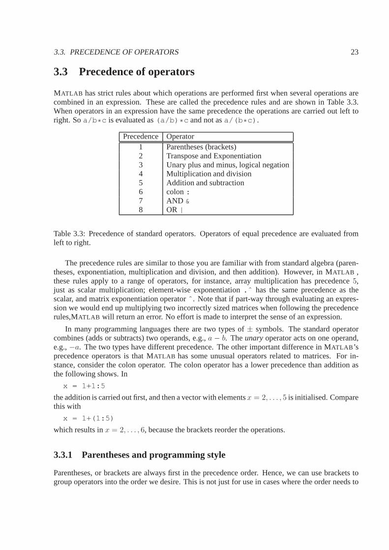
3.3 Precedence of operators
MATLAB has strict rules about which operations are performed first when several operations arecombined in an expression. These are called the precedence rules and are shown in Table 3.3.When operators in an expression have the same precedence theoperations are carried out left toright. Soa/b * c is evaluated as(a/b) * c and not asa/(b * c) .
Precedence Operator1 Parentheses (brackets)2 Transpose and Exponentiation3 Unary plus and minus, logical negation4 Multiplication and division5 Addition and subtraction6 colon :7 AND &8 OR |
Table 3.3: Precedence of standard operators. Operators of equal precedence are evaluated fromleft to right.
The precedence rules are similar to those you are familiar with from standard algebra (paren-theses, exponentiation, multiplication and division, andthen addition). However, in MATLAB ,these rules apply to a range of operators, for instance, array multiplication has precedence5,just as scalar multiplication; element-wise exponentiation .ˆ has the same precedence as thescalar, and matrix exponentiation operatorˆ . Note that if part-way through evaluating an expres-sion we would end up multiplying two incorrectly sized matrices when following the precedencerules,MATLAB will return an error. No effort is made to interpret the senseof an expression.
In many programming languages there are two types of± symbols. The standard operatorcombines (adds or subtracts) two operands, e.g.,a − b. Theunaryoperator acts on one operand,e.g.,−a. The two types have different precedence. The other important difference in MATLAB ’sprecedence operators is that MATLAB has some unusual operators related to matrices. For in-stance, consider the colon operator. The colon operator hasa lower precedence than addition asthe following shows. In
x = 1+1:5
the addition is carried out first, and then a vector with elementsx = 2, . . . , 5 is initialised. Comparethis with
x = 1+(1:5)
which results inx = 2, . . . , 6, because the brackets reorder the operations.
3.3.1 Parentheses and programming style
Parentheses, or brackets are always first in the precedence order. Hence, we can use brackets togroup operators into the order we desire. This is not just foruse in cases where the order needs to

24 CHAPTER 3. MATLAB AS A BIG CALCULATOR
be changed. Using brackets can often be useful even where theorder is already correct, because itcan make an expression much easier to read, and debug. As such, using brackets sensibly to makecomplex expressions more readable is a part of good coding practice.
3.4 Vectorisation of formulae
Array operations can be used to evaluate a formula repeatedly for a large amount of data. Let’sconsider the following formula for calculating compound interest.
Example: An amount of moneyA is invested over a period ofn years with an annual interestrate r. After n years we have an amountA(1 + r)n. Suppose we want to calculate the finalbalances for investments of$750, $1000, $3000, $5000 and$11, 999 over ten years, with an annualinterest rate of9%. The following sequence of commands does the calculation byusing an arrayoperations on a vector which contains the initial investments:
format bankA = [750 1000 3000 5000 11999];r = 0.09;n = 10;B = A * (1+r)ˆn;disp ([A’ B’])
The output is
750.00 1775.521000.00 2367.363000.00 7102.095000.00 11836.82
11999.00 28406.00
Notes:
1. format bank provides a two-decimal-place fixed format for currency.
2. In the statementB=A* (1+r)ˆn , the expression(1+r)ˆn is evaluated first because expo-nentiation has a higher precedence than multiplication. This is a scalar operation.
3. After that the array operation between the vectorA and the scalar(1+r)ˆn is formed.
4. A * may be used instead of a. * because the array multiplication is between a scalar and anon-scalar (although. * would not be wrong).
5. A table is displayed, with columns given by the transposesof A andB.
The process of writing out a formula such that we can calculate it for a vector of inputs is calledvectorisationof a formula. Vectorization of MATLAB code is very important. MATLAB has beencarefully optimized for vector and matrix operations, and will do these very quickly (almost asquickly as purpose written C-code). Other types of operations are not as fast, as we shall see later.

3.4. VECTORISATION OF FORMULAE 25
Example: Often we want to compute much more complicated formulae, fora range of inputs.For instance, let us compute the following formulae for calculating the value of a European calloption (using the Black-Scholes model). A European call option on a share gives us the right tobuy a share of the stock at priceK afterT years. The Black-Scholes formula gives its predictedvalue at
C = SΦ(d1) − Ke−rT Φ(d2),
whereΦ(·) is the standard normal cumulative distribution function.
d1 =ln(S/K) + (r + σ2/2)T
σ√
T
d2 =ln(S/K) + (r − σ2/2)T
σ√
TS = current price of the stock
T = time till option is exercised
K = exercise price
r = interest rate
σ = volatility
Obviously this is rather complicated if we wanted to computeby hand, but we can calculate thevalue of the option for a variety of exercise pricesK using the simple MATLAB code
% set the problem parametersS = 1, r = 0.07, sigma = 1, T = 3;K = 0:0.1:2;d1 = (log(S./K) + (r-sigmaˆ2)/2)/(sigma * sqrt(T));d2 = (log(S./K) + (r-sigmaˆ2)/2)/(sigma * sqrt(T));C = S * normal_cdf(d1) -exp(-r * T) * K . * normal_cdf(d2)plot(K, C);
where we will describe how to define the functionnormal_cdf(x) in Section 8.2.3. Noticethat we put. * and./ operators in the places where we could be operating on vectors. The resultis a graph (shown in Figure 3.1) showing us the behaviour of the option values, from which wecan assess what we would be willing to pay for such an option.
0 0.5 1 1.5 2−0.2
0
0.2
0.4
0.6
0.8
1
1.2
K
C
Figure 3.1: Option prices

26 CHAPTER 3. MATLAB AS A BIG CALCULATOR

Chapter 4
Input/Output
Often we need to either obtain input to our program from the user, or from a file, or output in-formation to the user or a file. We have already seen two approaches to sending output to theMATLAB window.
1. With thedisp function, e.g.disp(x) .
2. By entering a variable name, assignment or expression on the command line, without asemi-colon;
In this chapter we will provide more details of these approaches, but also we will introduce otherapproaches to I/O (Input/Output).
4.1 disp
The general form ofdisp for a numeric variable is
disp( variable )
To display a message and a numeric value on the same line we usethe following technique:
x=2;disp( [’The answer is ’, num2str(x)] )
The output should be
The answer is 2
We want to display acharacter stringand a number but the elements of a MATLAB vector mustbe either all numbers or all strings. To overcome this we convert the numberx to its stringrepresentationusing the functionnum2str , and the square brackets ([ ] ) concatenate the twostrings to form one string which is displayed.
27

28 CHAPTER 4. INPUT/OUTPUT
4.2 Theformat statement
MATLAB has the following two basic rules:
1. It always attempts to display integers (whole number) exactly. If the integer is too large it isdisplayed in scientific notation with five significant digits, e.g 1 234 567 890 is displayed as1.2346e+09 (i.e 1.2346 × 10⁹).
2. Numbers with decimal parts are displayed with four significant decimal digits. If the valueof x is in the range0.001 < x ≤ 1000 it is displayed in fixed point form, otherwise scientific(floating point) notation is used e.g. 1000.1 is displayed as1.0001e+003 .
Note that numbers are not displayed to the precision they arecomputed to.
This is MATLAB ’s default format. It is possible to change to format for output. To outputnumbers displaying more significant digits useformat long , or format bank can be used tooutput currency to two decimal places. There are many other options, seehelp format for details.However, complete control over the output format requires us to use thefprintf function.
4.3 fprintf
Thefprintf statement is much more flexible thandisp . Consider the example
balance = 12345;rate = 0.09;interest = balance * rate;balance = balance + interest;fprintf( ...
’Interest rate: %6.3f New balance: %8.2f\n’, ...rate, balance )
If we run this our output should look like
Interest rate: 0.090 New balance: 13456.05
The fprintf function has allowed us to control the format of the output precisely. More gener-ally, we might callfprintf using
fprintf (’ format string’, list of variables)
The format stringcontrols how the output appears. It may contain a simple textstring, in whichcase this is printed out. It may also contain one of a series ofcodes (mixed into the text), and thesespecial codes are replaced (in the output) with either a special character, or the value of one of thevariables in the list of input arguments. Table 4.1 gives a list of common codes.
Note the following:
1. In the case of%eand%f thefield widthand number of decimal places or significant figuresmay be specified immediately after the%. For instance we might write

4.3. FPRINTF 29
Code Action%f write a numerical variable in decimal notation%e write a numerical variable in scientific notation%g write a numerical variable (MATLAB ’s choice)%s write a string variable%% the % sign\n new line\t horizontal tab\b backspace\\ \
Table 4.1: Special codes used byfprintf
• %8f which means the width of the output will be 8 characters (and extra space will bepadded at the left to fill in gaps).
• %.3f which means write the number out showing three decimal places. By default%fmeans%.6f .
• %6.1f which means write the number with width 6, and one decimal place.
• %12.3e means scientific notation over 12 columns altogether (including the decimalpoint, a possible minus sign and four for the exponent) with 3digits in the mantissaafter the decimal point.
Note that numbers are rounded off when outputting with limited precision.
2. The%gspecifier is mixed and leaves it up to MATLAB to decide exactly what format to use.
3. The%s specifier also allows you to specify the width of the output string (padded withspaces if the string is not wide enough), e.g.%6s.
4. Thelist of variablescontains values that we wish to output.
5. Note that fprintf can take a vector as an input variable, and will recycle the format stringuntil the the elements of the input are all used (they are usedcolumnwise).
6. We often end a format string with\n in order to start the next output on a new line.
Table 4.2 shows a series of examples offprintf functions illustrating some of these options.
There are a number of otherconversion characters(characters following a % sign), andescapecodes(characters following a backslash\ ), but we will not consider them in detail here. It isnoteworthy that the syntax offprintf in MATLAB is similar to that used inC, and the twoduplicate many escape codes and conversion characters.
4.3.1 Output to a file with fprintf
Output may be sent to a file withfprintf . To do so we need toopenthe file for writing with thefopen function. This will create afile identifier, or FID variable. For example:

30 CHAPTER 4. INPUT/OUTPUT
function call outputfprintf(’Hello, world!\n’) Hello, world!
fprintf(’pi = %f\n’, pi) pi = 3.141593fprintf(’pi = %.12f\n’, pi) pi = 3.141592653590fprintf(’pi = %10.6f\n’, pi) pi = 3.141593fprintf(’pi = %e\n’, 100 * pi) pi = 3.141593e+02fprintf(’pi = %g\n’, 100 * pi) pi = 314.159
fprintf(’x = %.0f\n’, 1:3) x = 1x = 2x = 3
fprintf(’x = %3.0f, y = %.3f\n’, -1, sqrt(2)) x = -1, y = 1.414
fprintf(’message = %s\n’, ’hello’) message = hello
Table 4.2: Examples offprintf . The first is just printing a string, the second group showdifferent number formats, and the third shows the recyclingof the format string when the inputvariable is a vector.
fid = fopen(’exp.txt’,’w’);
The first input argument tofopen is the name of the file we wish to write to. The second inputargument’w’ specifies that it is to be opened forwriting. Thefopen function has lots of otheroptions. Usehelp fopen to find out more.
Thefprintf command takes an extra input argument, which is the FID variable, in this casefid , which tellsfprintf to output the results to the file. For example,
x = 0:.1:1;y = [x; exp(x)];fid = fopen(’exp.txt’,’w’);fprintf(fid,’%6.2f %12.8f\n’,y);fclose(fid);
After writing the output to the file we need toclosethe file with thefclose function. Note thatwe can give the FID variable any (allowed) variable name, andhave more than one open file at atime. We can even have an array of FID variables.
Note thatfopen can also be used to open a file for reading (or several other options). Whenreading a file, we might use thefscanf function but there is often a better approach.
4.3.2 sprintf
Sometimes it is desirable to create a string, including variables. We can use thesprintf functionto do this. The function is called just asfprintf , but it has one output argument, which is the

4.3. FPRINTF 31
result of the combination of formatted string output. For instance
the_string = sprintf(’pi = %f\n’, pi)
Will result in the_string holding the value’pi = 3.141593’ . This type of constructioncan often be useful for creating title plots, for instance, consider the following code that creates aplot, with a title that depends on the value off .
f = 3;x = 1:0.01:10;y = sin(f * x);plot(x, y);title_str = sprintf(’f = %f\n’, f);title(title_str);
4.3.3 Theinput command
Let’s rewrite the script filecalc interest.m so that it looks like
balance = input( ’Enter bank balance: ’ );rate = input( ’Enter interest rate: ’ );interest = rate * balance;balance = balance + interest;format bankdisp( ’New Balance:’ )disp( balance )
If we now enter the script file name, which I’ve calledcalc interest1.m at the prompt we areinterrogated by the computer for the initial values of the balance and interest rate. The commandwindow will contain the following lines:
>> calc_interest1Enter bank balance: 1000Enter interest rate: 0.15New Balance:
1150.00
The input statement provides a more flexible way of getting data into a program. It allows us toenter datawhile a script is running.
The general form of theinput statement is
variable= input( ’ prompt’ )
1. prompt is a message which prompts the user for the values(s) to be entered. It must beenclosed in apostrophes (single quotes).
2. A semi-colon at the end of theinput statement will prevent the value entered from beingimmediately echoed on the screen.

32 CHAPTER 4. INPUT/OUTPUT
3. Vectors and matrices may also be entered withinput , as long as you remember to enclosethe elements in square brackets.
4. Strings may be input if they are enclosed in quotes, e.g.,
name = input( ’Enter your name: ’ );fprintf(’Hello %s!\n’, name);
we would see a prompt and enter our name as follows:
Enter your name: ’John’Hello John!
4.4 Advanced I/O
MATLAB has many commands for more advanced Input/Output. A common requirement is toread data from a file. Simple text files are the easiest to read.MATLAB supports this in a varietyof ways the most general being thefscanf function, which is similar to the function of the samename inC.
However, we can use an simple approach when a data file is really a table, i.e., it consists ofa series of lines, each of which is in a fixed format. More specifically, row i of the file lookssomething like
datai1, datai2, datai3, ..., dataiN
where for a given columnj, each of the termsdataij is the same type of data (number or string).In this case we can use thetextread function. We call this function as follows:
[data1, data2, ..., dataN] = textread( file, format_str);
The file is the file from which we wish to read, and the format string specifies whether the datais a string, number, of some other type of data. Each of the output variables would contain onecolumn of the data from the file, i.e., for a file withm rowsdata1 = (data11, . . . , datam1)
′.
The functiontextread has many optional arguments to, for instance, change the delimiterbetween data in each row, or to allow for header lines, or comments in the file. For instance,assume we have a fileaddresses.dat as follows:
% format:% last name, first name, address, agePotter,Harry,Hogworts,17The Grey,Gandalf,Middle Earth,1023Christmas,Father,North Pole, 2008
We could read this file using the commands

4.4. ADVANCED I/O 33
file = ’addresses.dat’;format_str = ’%s %s %s %f’;[last_name, first_name, address, age] = ...
textread(file, format_str, ...’commentstyle’, ’matlab’, ...’delimiter’, ’,’);
The optioncommentstyle allows us to specify that strings beginning with % are comments(just as they are in a MATLAB program), and thedelimiter option specifies that the file is inCSV format. The data itself would be read into the variables with the corresponding names. Forinstance, the variableage would be a column vector containing[17; 1023; 2008] .
Many files can be read usingtextread and various related functions. However, these are alltext files that basically consist of a series of characters. Abinary file, consists of a series of 1’sand 0’s in a format that is (i) often optimized to reduce spacerequirements, and (ii) depends onthe type of data being held. Common examples include Excel’sfile format, along with commonmedia files such as music and video files. MATLAB has many functions for reading, writing anddisplaying such data. We will not examine these at length except to note some of the possibilities:
• Audio: MATLAB can read several file formats, but the easiest and most commonare.wavfiles, which can be read/written and played using thewavread , wavwrite andwavplayfunctions.
• Images: Image in many formats (e.g.,.png , .jpg , .tiff , etc.) can be read into MATLAB
usingimread , written usingimwrite and displayed using theimage functions.
• Excel: Excel files can be read and written usingxlsread andxlswrite .
• Video: .avi video files can be read and written usingaviread andmovie2avi , re-spectively.
Thehelp command can provide further information about all of these functions, and additionalI/O functions can be found usinghelp iofun .

34 CHAPTER 4. INPUT/OUTPUT

Chapter 5
Program flow control
We have seen earlier that MATLAB statements are usually executed in the order we type them,either in the command window, or in a.m script file. However, sometimes we want the order orexecution of statements to change, perhaps depending on thevalue of a variable. We might wantcertain statements to only run under some circumstances, orto run multiple times. Programflowcontrol refers to the programming constructions used to achieve this type of reordering.
MATLAB is a high-level language, which means that it is intended to look a little like a naturalhuman language — in particular English — combined with standard mathematical formulas. Untilnow we have mainly concentrated on the mathematical component, but we will now examinesome of the “English-like” syntax used in MATLAB that are used to control program flow, inparticular thekeywordsif , else , end , for andwhile . More information can be found usingthehelp lang command.
5.1 Making decisions withif
A standard requirement isconditional execution, i.e., we only want to execute some piece of codeif a condition is true. The condition could depend on previous calculations, and so we don’t knowthe result when we are writing the program. We only learn whether the condition holds when theprogram executes. We typically achieve this type of conditional execution using theif statement.
For example, the MATLAB function rand generates a random number in the range0 − 1.What would we expect if we were to enter the following commands?
r = rand;if r > 0.5
disp(’greater indeed’)end
In the second statement we have usedif and a relational operator>. MATLAB will only displaythe messagegreater indeed if r is greater than 0.5.
35

36 CHAPTER 5. PROGRAM FLOW CONTROL
5.1.1 Theif statement
The simplest form of theif statement is
if conditionstatements
end
We note the following points:
1. conditionis usually alogical expression, i.e. an expression containing logical operators suchas are found in Table 3.2. Typically it might involve one or more relational (comparison)operators, combined with logical operations like AND and OR.
2. If conditionis true,statementis executed but ifconditionis false, nothing happens.
3. The condition should typically be a scalar. If it is a vector or matrix, it is considered trueonly if all elements of the matrix are true. A single zero element in a vector or matrix rendersit false.
Simple examples of condition are
MATLAB condition meaningbˆ2<4 * a* c b2 < 4acx>=0 x ≥ 0a˜=0 a 6= 0bˆ2==4 * a* c b2 = 4acx >= 0 & x < 5 0 ≤ x < 5
5.1.2 Theif-else statement
Consider the following example:
x = 2;if x < 0
disp( ’negative’ )else
disp( ’non-negative’ )end
This tests to see ifx is negative. If it is it will return the messagenegative , if it is positive orzero it will return the messagenon-negative .
Most banks offer differential interests rates. Suppose that the rate is 9% if the amount of yoursavings is less than $5000 but 12% otherwise. Given a starting balance, we can calculate our newbalance using the following program:
% test whether balance is less than 5000if balance < 5000
% if it is set the interest rate to be 0.09
5.1. MAKING DECISIONS WITHIF 37
rate = 0.09else
% balance is greater than or equal to 5000% set the interest rate to be 0.12rate = 0.12
end
% calculate and display the new balancenew_balance = balance + rate * balance;disp(’New balance after interest paid is:’)format bankdisp( new_balance )
The basic form ofif-else for use in a program file is
if conditionstatements1
elsestatements2
end
Note the following:
1. Bothstatements1andstatements2represent one or more statements.
2. If the condition is true,statements1are executed, but if the condition is false,statements2are executed. This is how we force MATLAB to choose between two alternatives, and inprogramming it is often callbranching.
3. Theelse part is optional. Theif statement is a special case of theif-else statement.
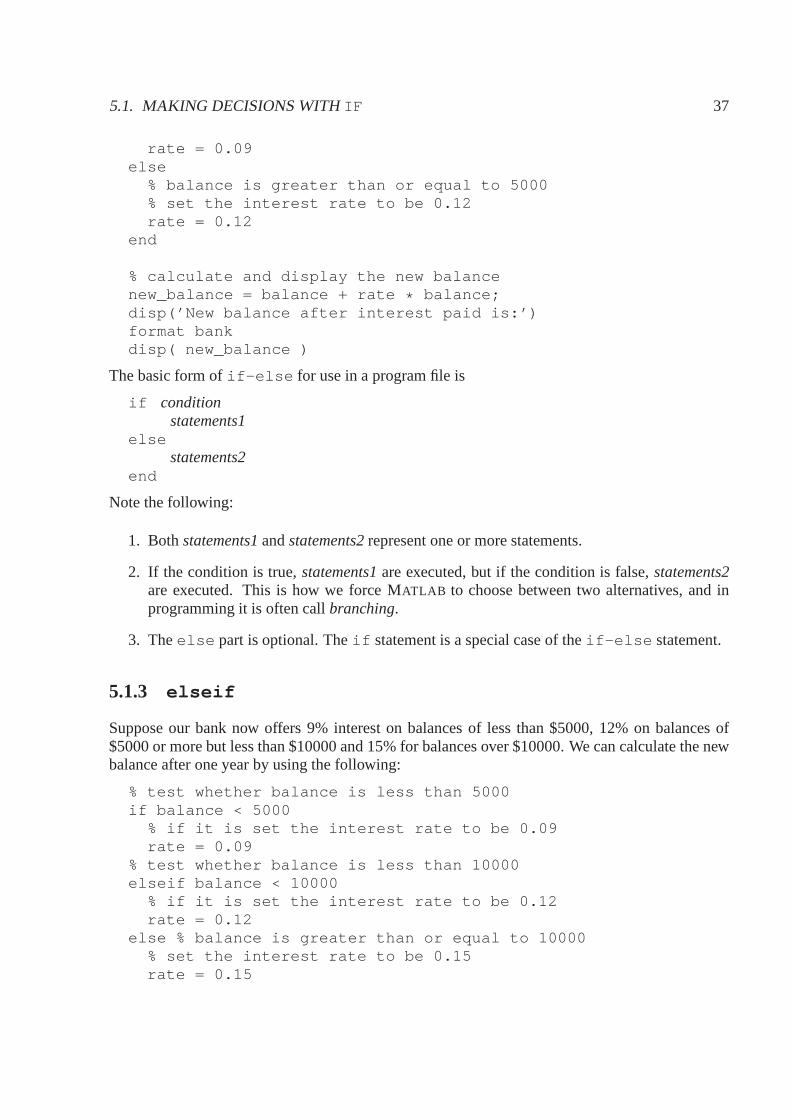
5.1.3 elseif
Suppose our bank now offers 9% interest on balances of less than $5000, 12% on balances of$5000 or more but less than $10000 and 15% for balances over $10000. We can calculate the newbalance after one year by using the following:
% test whether balance is less than 5000if balance < 5000
% if it is set the interest rate to be 0.09rate = 0.09
% test whether balance is less than 10000elseif balance < 10000
% if it is set the interest rate to be 0.12rate = 0.12
else % balance is greater than or equal to 10000% set the interest rate to be 0.15rate = 0.15

38 CHAPTER 5. PROGRAM FLOW CONTROL
end
% calculate and display the new balancenew_balance = balance + rate * balance;disp(’New balance after interest paid is:’)format bankdisp( new_balance )
In general theelseif clause is used as follows:
if condition1statements1
elseif condition2statements2
elseif condition3statements3
...else
statementsNend
We sometimes call this anelseif ladder. It works as follows:
1. condition1is tested. If it is truestatements1are executed; MATLAB then moves to the nextstatement afterend .
2. If condition1is false, MATLAB checkscondition2. If it is true, statements2are executed,followed by the statements afterend .
3. In this way, all the conditions are tested until a true condition is found. As soon as a truecondition is found no furtherelseif statements are examined and MATLAB jumps off theladder.
4. If none of the conditions are true,statementsNafterelse are executed.
5. There can be any number ofelseif ’s but at most oneelse .
6. elseif must be written as one word.
7. if andif-else statements are special cases of theif-elseif-else statement.
5.1.4 Logical operators
Logical expressions can be constructed using thethree logical operators& (and),| (or), ˜ (not),that we examined earlier. For example the quadratic equation
ax2 + bx + c = 0,
has equal roots, given by−b/(2a), provided thatb2 − 4ac = 0 anda 6= 0. This can be translatedto the following MATLAB statements:
5.1. MAKING DECISIONS WITHIF 39
if (bˆ2 - 4 * a* c == 0) & ( a ˜= 0)x = -b / (2 * a)
end
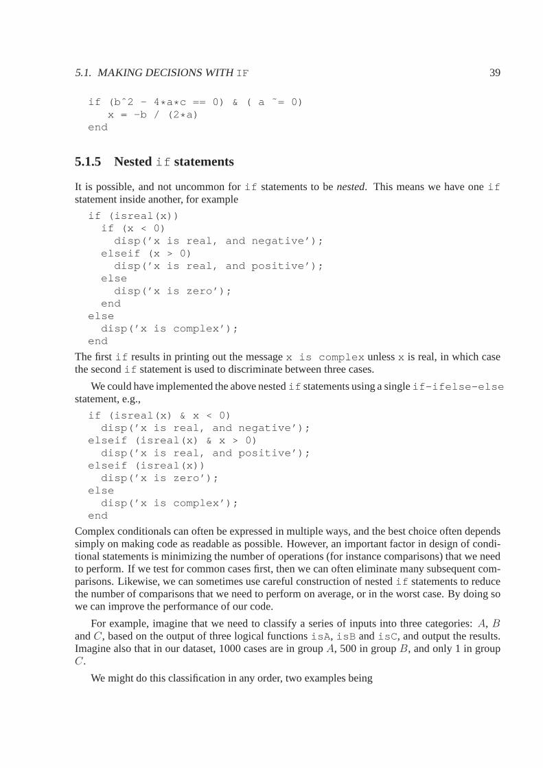
5.1.5 Nestedif statements
It is possible, and not uncommon forif statements to benested. This means we have oneifstatement inside another, for example
if (isreal(x))if (x < 0)
disp(’x is real, and negative’);elseif (x > 0)
disp(’x is real, and positive’);else
disp(’x is zero’);end
elsedisp(’x is complex’);
end
The first if results in printing out the messagex is complex unlessx is real, in which casethe secondif statement is used to discriminate between three cases.
We could have implemented the above nestedif statements using a singleif-ifelse-elsestatement, e.g.,
if (isreal(x) & x < 0)disp(’x is real, and negative’);
elseif (isreal(x) & x > 0)disp(’x is real, and positive’);
elseif (isreal(x))disp(’x is zero’);
elsedisp(’x is complex’);
end
Complex conditionals can often be expressed in multiple ways, and the best choice often dependssimply on making code as readable as possible. However, an important factor in design of condi-tional statements is minimizing the number of operations (for instance comparisons) that we needto perform. If we test for common cases first, then we can ofteneliminate many subsequent com-parisons. Likewise, we can sometimes use careful construction of nestedif statements to reducethe number of comparisons that we need to perform on average,or in the worst case. By doing sowe can improve the performance of our code.
For example, imagine that we need to classify a series of inputs into three categories:A, BandC, based on the output of three logical functionsisA , isB andisC , and output the results.Imagine also that in our dataset, 1000 cases are in groupA, 500 in groupB, and only 1 in groupC.
We might do this classification in any order, two examples being
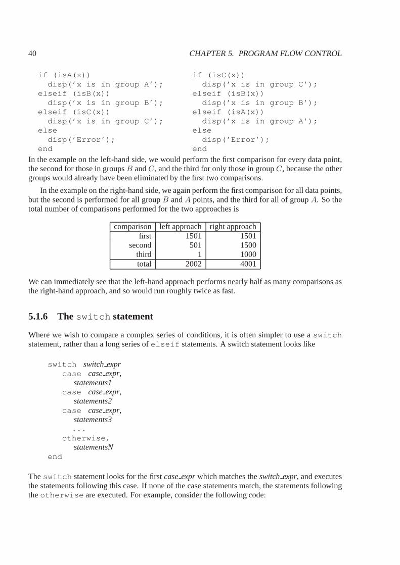
40 CHAPTER 5. PROGRAM FLOW CONTROL
if (isA(x)) if (isC(x))disp(’x is in group A’); disp(’x is in group C’);
elseif (isB(x)) elseif (isB(x))disp(’x is in group B’); disp(’x is in group B’);
elseif (isC(x)) elseif (isA(x))disp(’x is in group C’); disp(’x is in group A’);
else elsedisp(’Error’); disp(’Error’);
end end
In the example on the left-hand side, we would perform the first comparison for every data point,the second for those in groupsB andC, and the third for only those in groupC, because the othergroups would already have been eliminated by the first two comparisons.
In the example on the right-hand side, we again perform the first comparison for all data points,but the second is performed for all groupB andA points, and the third for all of groupA. So thetotal number of comparisons performed for the two approaches is
comparison left approach right approachfirst 1501 1501
second 501 1500third 1 1000total 2002 4001
We can immediately see that the left-hand approach performsnearly half as many comparisons asthe right-hand approach, and so would run roughly twice as fast.
5.1.6 Theswitch statement
Where we wish to compare a complex series of conditions, it isoften simpler to use aswitchstatement, rather than a long series ofelseif statements. A switch statement looks like
switch switchexprcase caseexpr,
statements1case caseexpr,
statements2case caseexpr,
statements3...
otherwise,statementsN
end
Theswitch statement looks for the firstcaseexprwhich matches theswitchexpr, and executesthe statements following this case. If none of the case statements match, the statements followingtheotherwise are executed. For example, consider the following code:

5.2. REPETITION WITHFOR 41
grade = input(’Enter your grade (F,P,C,D,HD):’);switch grade
case ’F’fprintf(’Your mark was < 50\n’);
case ’P’fprintf(’Your mark was between 50 and 65\n’);
case ’C’fprintf(’Your mark was between 65 and 75\n’);
case ’D’fprintf(’Your mark was between 65 and 75\n’);
case ’HD’fprintf(’Your mark was > 85\n’);
otherwise,fprintf(’Error: %s was not a valid grade\n’, grade);
end
The response of the program to an input like’D’ would beYour mark was between 65 and 75 ,and it outputs an error if an invalid grade is input. Note alsothat the comparison works betweenstrings (we have to input a string in quotes), whereas the comparison operator, e.g.grade == ’HD’would treat’HD’ as a vector and would therefore fail ifgrade was a vector with only one ele-ment. You can test multiple conditions in a switch/case statement by putting them in curly brackets,e.g.{’D’,’HD’} .
5.2 Repetition withfor
Computers are stupid (we have to be quite careful about what we tell them to do) but very fast.Furthermore, many numerical techniques are built around the idea of performing a simple opera-tion many times. As a result, a common requirement in programming is the ability to repeat codemore than once (often many times). Obviously we could type the same commands more than once,but this is annoying, and more importantly it is harder to debug (you have to make sure each copyof the commands is exactly the same). There is an easier way. Repeating the same code is callediteration.
The most common type of iteration (in MATLAB ) is count controllediteration where we createa counter, and iterate over certain values of the counter. InMATLAB we do this using theforstatement. The following code
for i = 1:3disp(i)
end
creates thecounteri and then iterates thedisp statement for each value of the counter in thespecifier1:3 . That is, we execute the loop three times, once for each valuei = 1, 2, 3. The outputwould be
1

42 CHAPTER 5. PROGRAM FLOW CONTROL
23
This type of high-level iteration construct was first used inFORTRANin 1956, though it wascalled aDO loop in FORTRAN. For many years,FORTRANwas the most important languagefor scientific computation applications, primarily because of these types of high-level constructswhich it pioneered.
5.2.1 An example: square roots via Newton’s Method
The square rootx of any positive numbera may be found using only the arithmetic operations ofaddition, subtraction and division viaNewton’s method. This is an iterative process that refinesan initial guess. The followingpseudo-codedescribes Newton’s method for calculating the squareroot ofa.
1. Initialisex to a/2
2. Repeat the following steps a number of times (6 say)
• Replacex by (x + a/x)/2
3. Stop
The MATLAB program to do this (for the casea = 2) follows. Note that we print out the value ofx at each iteration.
disp( ’Square roots via Newtons method’ )a = 2;format long;format compact;x = a/2;for i = 1:6
x = (x+a/x)/2enddisp( ’Matlab’’s value for sqrt(2) is: ’)disp( sqrt(2) )
The output (after making the format long and compact) is
x =1.500000000000000
x =1.416666666666667
x =1.414215686274510
x =1.414213562374690
x =

5.2. REPETITION WITHFOR 43
1.414213562373095x =
1.414213562373095Matlab’s value for sqrt(2) is:
1.414213562373095
The value ofx converges to a limit, which is√
a. Note that this is identical to the value returnedby the MATLAB functionsqrt .
5.2.2 The basicfor statement
The simple form of thefor loop isfor index = j:k
statementsend
The loop will be performed exactly once for each value ofindex from j, j + 1, j + 2, . . . , k, inorder. On completion, the variableindex contains the last value used.
The termindexcan be any valid variable, e.g.,i , a_variable , or counter , but cannottake the form-x , or any other invalid variable name.
5.2.3 More generalfor statements
More generally, we can perform afor loop over any vector, i.e.,for index = vector
statementsend
In this case, the loop is run once for index taking each element of the vector as a value (in orderthrough the vector). Typically the vector is constructed for thefor loop, e.g.,
for index = 1:10:51disp( [’index = ’ num2str(index)] )
end
which would construct the vector[1 11 21 31 41 51] , and then apply the loop, outputtingindex = 1index = 11index = 21index = 31index = 41index = 51
We can explicitly construct the vector before calling the loop, e.g.,index_values = 10.ˆ[1:3];for index = index_values
disp( [’index = ’ num2str(index)] )end

44 CHAPTER 5. PROGRAM FLOW CONTROL
which would run the loop once each with the values ofindex being10, 100 and1000 and output
index = 10index = 100index = 1000
If the vector is empty,statementsare not executed and control passes to the statement followingtheend statement. For instance,
for i = 5:0disp(i)
end
will not do anything, because the vector[5:0] is empty. The correct form of this would beto use[5:-1:0] . It is sometimes worth explicitly testing for an empty indexvector using theisempty function before entering a loop, and output an error if the vector would be empty.
Example: We can combineif andfor statements. Consider a bottle of wine at temperature25◦C, which is placed in a refrigerator where the ambient temperatureF is 10◦C. We want to findout how the temperature of the wine changes over a period of time. To do this we first need one‘fact’, namelyNewton’s Law of Coolingwhich states:
The rate of change of temperatureT within a body placed in an environment whoseambient temperature isF is proportional to the difference between the temperature ofthe body and the ambient temperature,T − F .
Mathematically this translates to (remembering thatrate-of-changewith respect to time is simplythe derivative of the function)
dT
dt= −K(T − F ). (5.1)
We note
1. K is a constant of proportionality which depends upon the insulating properties of the ma-terial, in our case the glass bottle, and also the thermal properties of the wine.
2. The constantK is positive, since ifT > F , so that the wine is hotter than the ambienttemperature, we expect it to cool and hence the rate of changeof the temperature must benegative.
A standard way of approaching problems of this type is to break the time period up into a numberof small steps, each of lengthdt. If Ti is the temperature at thebeginningof stepi, we can use asimpleEuler method to get fromTi to Ti+1.
This method relies on approximating the differential equation
dy
dt= f(y; t),
by the approximationyi+1 − yi
∆t= f(yi; ti).

5.2. REPETITION WITHFOR 45
For our cooling problem we have
Ti+1 = Ti − K∆t(Ti − F ).
The following MATLAB script implements this scheme:
% Variable initialisations.K = 0.05;ambient_temperature = 10;temperature = 25;start_time = 0;end_time = 100;
% Request input values.delta_t = input(’Input the computational interval, delta_ t:’ );output_interval = input(’Please input the output interval : ’ );if rem(output_interval,delta_t) ˜= 0
error(’The output interval must be a multiple of delta_t!’)end
time = start_time;disp( ’Time Temperature’ )disp( [time temperature] )
for time = start_time+delta_t : delta_t : end_timetemperature = temperature - K * delta_t * ...
(temperature-ambient_temperature);if rem( time, output_interval ) == 0
disp( [time temperature] )end
end
The functionrem computes a remainder. It is used to check thatoutput interval is aninteger multiple ofdelta t , and to display the results everyoutput interval minutes (whentime is an integer multiple ofoutput interval the remainder will be zero).
5.2.4 Nestedfor statements
As with if statements, it is common in programming tonestfor loops. This means placing onefor loop inside another. For instance, when we work with anN × M array of dataA, we mightuse a construction such as
N = 12;M = 12;for i=1:N
for j=1:M

46 CHAPTER 5. PROGRAM FLOW CONTROL
A(i,j) = i * j;end
end
The inner loop is executed once for each outer loop, so we willeventually iterate through allallowed values ofi andj.
5.2.5 Avoidingfor loops by vectorising
Suppose we want to evaluate1000000∑
n=1
1
n2.
There are two way to do this. Firstly using thefor loop
partial_sum = 0;for term = 1:1000000
partial_sum = partial_sum + 1 / termˆ2;enddisp( partial_sum )
We canvectorisethis command by using thesum command
terms = 1:1000000;partial_sum = sum(1 ./ terms.ˆ2)
In general, MATLAB is highly optimized for vectorized calculation. A vector/matrix computationsuch as the second approach will be much faster than the first.On my computer, the first approachtook 1.03 seconds, and the second approach tool only 0.048 seconds. The second approach wasmore than 20 times faster!
This type of speedup is most clear in large, nested loops. Forinstance, if we wished to computea large multiplication table, we could use the nested loop approach immediately above, or we coulduse the matrix approach described in Section 2.8. The latterapproach will be much faster.
This a key feature/problem with MATLAB . The fact that it can do matrix operations quicklyis of great value. However, it is not always easy to vectorisea complex program. Also, there is acost in memory – the vectorized approach requires us to storea large vector in memory, whereasthe nested loop approach can sometimes avoid this.
5.2.6 Preallocating arrays
An additional issue, when we use a loop, is preallocation of arrays. MATLAB ’s ability to allocatememory for arrays on the fly makes it convenient to simply create an array as we go through aloop, e.g., consider the following code to compute the Fibonacci sequence:
x(1) = 1;x(2) = 1;N = 10000;

5.2. REPETITION WITHFOR 47
for i=3:Nx(i) = x(i-1) + x(i-2);
end
Here the vectorx is extended in each iteration of the loop. However, when we know it size, it isoften more efficient to preallocate the array. For instance:
N = 10000;x = zeros(N,1);x(1) = 1;x(2) = 1;for i=3:N
x(i) = x(i-1) + x(i-2);end
This creates the array before we use it in the loop, and avoidsmemory management overheadinside the loop. In my version of MATLAB , the second approach is roughly ten times as fast. Notethat the above code could also be vectorized, given even better improvements in speed, but thereare some times when vectorization is not an option.
5.2.7 Non-deterministic repetition
The key feature of afor loop is that the loop repetition is deterministic in the sense that it ispredetermined at the start of the loop. The number of iterations may depend on earlier definedvariables. For example, we may set a variableNwhich is then used in creating thefor loop, e.g.,
for i = 1:Ndisp(i)
end
but care must be taken with afor loop to avoid tampering with the index variable inside the loop.If we explicitly change the value of the counter variable inside the loop the behaviour of the loopbecomes unspecified, and we won’t know what will happen in advance. So once the loop is startedwe (apparently) can’t stop it early. Certainly we shouldn’ttry to stop it by changing theindex .
However, there are two statements that allow us the varying the standard looping behaviour.The first allows early breakout from the loop: thebreak statement will drop us out of a loopearly. It is usually used in conjunction with a conditional statement to cause early breakout from aloop in special circumstances, e.g.,
for i=1:1000000x = some_complex_function(x, i);if (isnan(x))
break;end
end
This loop repeatedly changes the value ofx based on its previous value, and the value of thecounter variablei . However, if there is a problem and the function returnsNaN, then we breakout of the loop prematurely in order to avoid many needless repetitions of the loop.

48 CHAPTER 5. PROGRAM FLOW CONTROL
Thebreak statement should be used with considerable caution as it canreduce readability ofcode significantly.
The other related statement is thecontinue statement, which passes the loop onto its nextvalue, skipping any remaining statements, e.g.
for i=1:6if (mod(i,2) == 0)
continue;enddisp(i);
end
would output
135
Even terms are omitted from the output, even though we loop over all terms, because thecontinuestatement is executed in these cases, and hence subsequent statements (e.g. thedisp statement)are avoided for even values ofi . Once again,continue statements should be used with carebecause of readability concerns. Frequent use ofbreak andcontinue can result inspaghetticode.
And there is a better approach, using non-deterministic repetition via awhile loop.
5.3 Non-deterministic repetition with while
Suppose we want to use a loop but we don’t know how long it will runbefore we startthe loop. Itis common that we want to run a numerical algorithm until it hasconvergedwhere we won’t knowhow long this will take until we run the algorithm. We call this acondition controlledloop. Thenumber of executions of the loop will be controlled some condition calculated within the loop,rather than by a simple counter defined as part of the loop.
A simple example of this type of loop is the following game. MATLAB ‘thinks’ of a numberbetween1 and10 and we have to guess it. If our guess is too high or too low then the script mustsay so, and then give us another go. If our guess is correct then the script should congratulate us.
Here’s the pseudo-code for the problem
1. Generate a random number.
2. Prompt the user for a guess.
3. While the guess is wrong:
• If the guess is too low
– Tell the user it is too low
• Otherwise
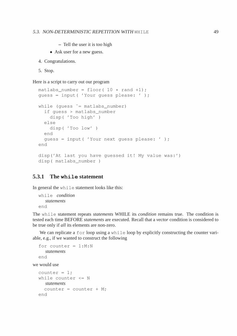
5.3. NON-DETERMINISTIC REPETITION WITHWHILE 49
– Tell the user it is too high
• Ask user for a new guess.
4. Congratulations.
5. Stop.
Here is a script to carry out our program
matlabs_number = floor( 10 * rand +1);guess = input( ’Your guess please: ’ );
while (guess ˜= matlabs_number)if guess > matlabs_number
disp( ’Too high’ )else
disp( ’Too low’ )endguess = input( ’Your next guess please: ’ );
end
disp(’At last you have guessed it! My value was:’)disp( matlabs_number )
5.3.1 Thewhile statement
In general thewhile statement looks like this:
while conditionstatements
end
The while statement repeatsstatementsWHILE its condition remains true. The condition istested each time BEFOREstatementsare executed. Recall that avectorcondition is considered tobe true only ifall its elements are non-zero.
We can replicate afor loop using awhile loop by explicitly constructing the counter vari-able, e.g., if we wanted to construct the following
for counter = 1:M:Nstatements
end
we would use
counter = 1;while counter <= N
statementscounter = counter + M;
end

50 CHAPTER 5. PROGRAM FLOW CONTROL
In this example we explicitly create thecounter variable, and increment it by the requiredamountM at each loop. Thefor loop construction is more concise, and so often preferred, butthewhile loop form allows more flexibility in combining both count controlled, and conditioncontrolled looping.
5.3.2 Infinite loops
One of the dangers of a condition controlled loop is that the condition will remain true forever.In this case the loop will continue indefinitely. We call thisan infinite loop, and it will resultin a program that doesn’t terminate naturally. For instance, the following program will executeindefinitely,
while (1)disp(’Hello, world!’);
end
The program will repeatedly output “Hello, world!” becausethe condition1 is always true (re-member that in MATLAB 1 stands for the logical TRUE). In MATLAB we can stop a program byexiting MATLAB , or by typingCtrl-C , which sends an interrupt signal to MATLAB . WhenMATLAB receives such a signal it should stop what it is doing. It willstop normal execution of aprogram, or even the infinite loop above.
Occasionally an infinite loop can be useful. Sometimes we want a program to perform someaction until the program is halted (by some outside interrupt). This type of programming fallsoutside the scope of this course.
5.4 Programming style
Whenever we have a conditional, or loop, it is wise to indent the code inside the loops (much as wehave done above). This greatly enhances the readability of the code by showing which parts willbe executed (conditionally, or iteratively). Where there are multiply nest loops or conditionals,then use multiple levels of indentation. MATLAB ’s editor will do this for you, but other editorsmay not do it automatically (for instance when you are codingC there is no built in editor).
Sometimes, if the code inside a conditional or loop is long (say longer than one page roughly)then we might also add a comment to theend statement, to help indicate which conditional orloop it is associated with. This can make debugging some codeeasier. For instance, we mightwrite
if (A > B)statement1statement2
...statementN
end % if (A > B)

5.5. OTHERMATLAB STATEMENTS 51
The comment% if (A > B) indicates which conditional theend statement is finishing.
On another point, I prefer to place conditionals inside brackets (forif andwhile statements).This is not generally necessary, but I find that it separates the logic of the condition from thesyntactical components and makes the result more readable.
5.5 Other MATLAB statements
MATLAB has a number of additional programming statements for flow control, mirroring manymodern programming languages. For instance
• try andcatch
• error
• assert
• return
These will not be covered in this course, but it is perhaps useful to know they exist. More infor-mation can be found usinghelp lang or help command.

52 CHAPTER 5. PROGRAM FLOW CONTROL

Chapter 6
Commonly used functions and variables
MATLAB has a large number of useful constants and functions rangingfrom mathematical func-tions to those for manipulating strings. Here we will present a quick summary of a number of themost commonly used. Much more detail on a function can be found by typinghelp , followed bythe function’s name. If you are trying to find a function, but don’t know its name thelookforcommand can often find it by searching for MATLAB commands that either match the search string(given as an input), or whose first line of description matches the search string.
6.1 ConstantsMATLAB has a number of pre-defined constants.
Constant name Valuepi πi
√−1
j√−1
eps the distance from 1.0 to the next larger double precision numberrealmax largest positive floating point numberrealmin smallest positive floating point numberfalse 0 (logical)true 1 (logical)
Note that “constants” are really just variables (in MATLAB ) and so can be easily redefined. Alsonote that irrational numbers can only be approximately represented, so constants such asπ areonly accurate to machine precision. Some standard constants such ase are not defined, but areeasily calculated, for instancee = exp(1). Some of the above constants are actually functions,e.g.,eps(x) gives the the positive distance from|x| to the next larger in magnitude floating pointnumber. There are also equivalent function torealmax andrealmin for integers.
53

54 CHAPTER 6. COMMONLY USED FUNCTIONS AND VARIABLES
6.2 Elementary Mathematical Functions
Here we present some of MATLAB ’s elementary mathematical functions. Note that if the argumentof a function is a vector (or array), the function is applied element by element to the values of thevector, e.g.
sqrt( [1 4 9 16] )returns
1.0000 2.0000 3.0000 4.0000Function list
Function Effectabs(x) absolute value ofx .acos(x) arc cosine (inverse cosine) ofx (returns a value between0 andπ).acosh(x) inverse hyperbolic cosine ofx , i.e. ln(x +
√x2 − 1).
asin(x) arc sine (inverse sine) ofx (returns a value between−π/2 andπ/2).asinh(x) inverse hyperbolic sine ofx .atan(x) arc tangent ofx (returns a value between−π/2 andπ/2).atanh(x) inverse hyperbolic tangent ofx .ceil(x) the smallest integer which is greater than or equal toxconj(x) complex conjugate ofx .cos(x) cosine ofx .cosh(x) hyperbolic cosine ofx .exp(x) value of the exponential functionex.factorial(n) n!.floor(x) the largest integer less than or equal toximag(x) returns theimaginarypart ofx .log(x) natural logarithm ofx .log2(x) base 2 logarithm ofx .log10(x) base 10 logarithm ofx .mod(x,k) x modk .nchoosek(n,k) the number of combinations
(
n
k
)
= n!/k!(n − k)!.rand random number in the interval[0, 1).real(x) thereal part ofxrem(x,y) remainder whenx is divided byy i.e.rem(19,5) returns4.round(x) rounds to the nearest integersign(x) the value−1, 0 or 1 depending upon whetherx is -ve, zero or +ve.sin(x) sine ofx .sinh(x) hyperbolic sine ofx .sqrt(x) square root ofx . This also handles negative or complex values.tan(x) tangent ofx .tanh(x) hyperbolic tangent ofx .
Note for trigonometric functions that angles are usually represented in radians, not degrees. Thereare versions of some trigonometric functions that act in degrees, e.g.cosd , however, it is generallybetter to convert to radians by multiplying by2π/360.
Seehelp elfun andhelp specfun for more mathematical functions, andhelp polyfunfor functions related to polynomials.

6.3. SIMPLE VECTOR/MATRIX FUNCTIONS 55
6.3 Simple Vector/Matrix functions
There are also a number of simple functions designed to be useful specifically with vectors ormatrices:
Function Effectdet(A) the determinant ofA.diag(A) get the diagonal entries of a matrixA.diag(x) construct a diagonal matrix withx along its main diagonal.diff(x) returns a vector containing differences of the input, i.e.,xi+1 − xi.eig(A) eigenvalues and vectors ofA.eye(N) construct theN x N identity matrix.find(x) find the indices where the logical vectorx=TRUEisempty(x) returns TRUE if the matrix/vector is empty.length(x) number of elements of vectorx .max(x) maximum element contained in the vectorx .mean(x) mean value of the elements in vectorx .min(x) minimum value contained in the vectorx .norm(A) the matrix norm ofA.ones(n,m) construct ann x m matrix of 1s.prod(x) product of the elements of vectorx .rand(n,m) construct ann x m matrix of rand .repmat(A,n,m) creates a new array withn × m blocks formed from matrixA.size(A) the number of rows and columns of a matrixA.std(x) the standard deviation of the elements ofx .sort(x) sorts elements of vectorx into ascending order.sum(x) sum of the elements of vectorx .trace(A) the trace ofA.zeros(n,m) construct ann x m matrix of 0s.
Many of the functions above have been described in terms of their vector version (e.g.sum, mean,max) but have a matrix version. Some likediag do something completely different with a matrixor a vector, whereas other just generalize the same operation. See the help for these functions formore details.
Additional functions can be found using the above help commands in addition tohelp matfunandhelp datafun . MATLAB also has a series of functions to deal with sparse matrices: moredetail can be seen withhelp sparfun .

56 CHAPTER 6. COMMONLY USED FUNCTIONS AND VARIABLES
6.4 Set functions
In MATLAB , we can choose to ignore order in a vector, and treat the vector like a set. There arespecial functions for operating on sets. A list of common setfunctions: (assuminga andb arevectors representing sets) follows.
Function Effectintersect(a,b) returns intersections of setsa andb.ismember(a,b) returns 0-1 array of the same size asa which indicates which values of
a are members ofb.setdiff(a,b) returns elements ofa that are not inb.setxor(a,b) returns elements ofa andb that are not in the intersection.union(a,b) returns union of setsa andb.unique(a) returns a list of the unique elements ofa.
6.5 Test functionsMATLAB has a number of functions designed to test certain conditions. The are commonly usedin conditionals.
Function Effectexist(name) test if a variable, function or filename exists.isempty(x) returns TRUE if the matrix/vectorx is empty.isnan(x) returns true ifx=NaNisinf(x) returns true ifx=Inf or x=-Infisfinite(x) returns true for any case except the above threeisreal(x) returns true ifx is real (not complex)strcmp(s1,s2) returns true if stringss1 ands2 are identicalisa(x, ’class_name’) tests if variablex is of class’class_name’isnumeric(x) tests if variablex is a numeric arrayislogical(x) tests if variablex is a logical arrayischar(x) tests if variablex is a character array (a string)ismember(a, s) tests if variablea is a member of sets
Typically these functions can operate on an array input, andreturn a logical array as output.
6.6 String functions
MATLAB has a number of functions specifically for dealing with strings (of characters). A list ofcommon string functions: (assumings , s1 ands2 are strings) follows.

6.7. DATES AND TIMES 57
Function Effectchar(x) convert an array of integersx into a string of characters.double(s) convert a strings to an array of integers.findstr(s1,s2) find the shorter of the two strings in the longer.lower(s) converts to lower case.strcat(s1,s2) concatenate two stringss1 ands2 .strcmp(s1,s2) returns true if stringss1 ands2 are identical.strtrim(s) remove insignificant whitespace froms .sprintf(...) similar tofprintf but returns a string.upper(s) converts to upper case.
The commandhelp strfun will list more possibilities, whilehelp strings reveals basicinformation about strings.
6.7 Dates and times
It is often useful to be able to work with times and dates, and MATLAB has a number of functionsfor doing so. Some simple time and date related functions are:
Function Effectclock returns a six element date vector of the form
[year month day hour minute seconds] .datenum(d) converts a date vectord into MATLAB ’s numerical representation of dates.datevec(x) converts an internal datex into a date vector.datestr(x) converts an internal datex into a human readable string.tic sets a “stopwatch” going.toc outputs the value of the stopwatch (in seconds).
Commands such astic and toc are useful for comparing computation times of alternative al-gorithms. Commands such asdatenum anddatestr have many alternative input and outputformats, and can be used quite flexibly to work with dates. When we wish to plot, for instance atimeseries, with dates along one axis, we use thedatetick command in conjunction with theabove.
6.8 Utility functions
We often need to interact with the file system/workspace of the computer we are operating on, andMATLAB has functions for doing so. Simple file system/workspace related functions

58 CHAPTER 6. COMMONLY USED FUNCTIONS AND VARIABLES
Function Effectclear remove variables from the workspace.cd(’d’) change working directory tod.dir(’d’) list the files in directoryd.load filename load variables from a.mat file.path(’p’) change the search path MATLAB uses to look for.m files.pause(n) pause a program forn seconds.pwd display the current working directory.save filename save all the workspace’s variables to a.mat file.what(’d’) list MATLAB specific files in a directory.who lists variables in the current workspace.whos lists variables in the current workspace in long form.
6.9 More information
One of the strengths of MATLAB is its many useful functions, we have listed only a fraction here.Use the appropriatehelp and lookfor commands to find more, as well as MATLAB ’s onlinedocumentation. The goal of this chapter has been to give you an idea of what is possible usingMATLAB ’s functions, rather than a complete list, or the details. The brief descriptions providedhere omit many important details, and you should examine thefunction in more detail before usingit (again using thehelp command, or the online documentation).
In addition, MATLAB has many “Toolboxes”, which can be purchased (or sometimes down-loaded) to add features to MATLAB , primarily by adding functions. Typing the commandverwill provide information on what version of MATLAB you have, and what toolboxes have beeninstalled. Additional help about these toolboxes is also available.
Finally, MATLAB also has many functions for displaying data, but we shall examine these inmore detail in the following section.

Chapter 7
Graphics
One of the most powerful features of MATLAB is its ability to visualize data using plots. The basicapproach is to use one of a set of functions to create a plot. Once created, features (such as axislabels) can be added to the plot either by function calls, or by interacting with the GUI of the plotwindow. We start this chapter by considering a basic 2D plot of a set of data.
7.1 Basic two-dimensional plots
The most common command to draw a single graph isplot , In its simplest form the commandtakes a single vector argument as inplot(y) . In this case the elements ofy are plotted againsttheir indices, e.g.
y=rand(1,20);plot(y);
plots20 random numbers against the integers1–20 joining successive points with straight lines asin figure 7.1(a).
Axes are automatically drawn, and the range of these is scaled to include the minimum andmaximum data points, but “nice” values of the extremes are chosen so that the plot will (hopefully)look good.
The most common form ofplot is plot(x,y) wherex and y are vectors of the samelength. The plot function uses the first argument as thex locations of data points, and the secondas they locations, and (by default) draws lines between the series of points. For example seeFigure 7.1(b), which shows the following example:
x = 0 : pi/40 : 4 * pi;y = sin(x);plot(x, y);
7.2 Decorating the figure
The figures above are not satisfactory. For instance, they have no axis labels, the text is small, andthe graphs are rather bland. In this section we discuss how tomodify and improve our graphs.
59
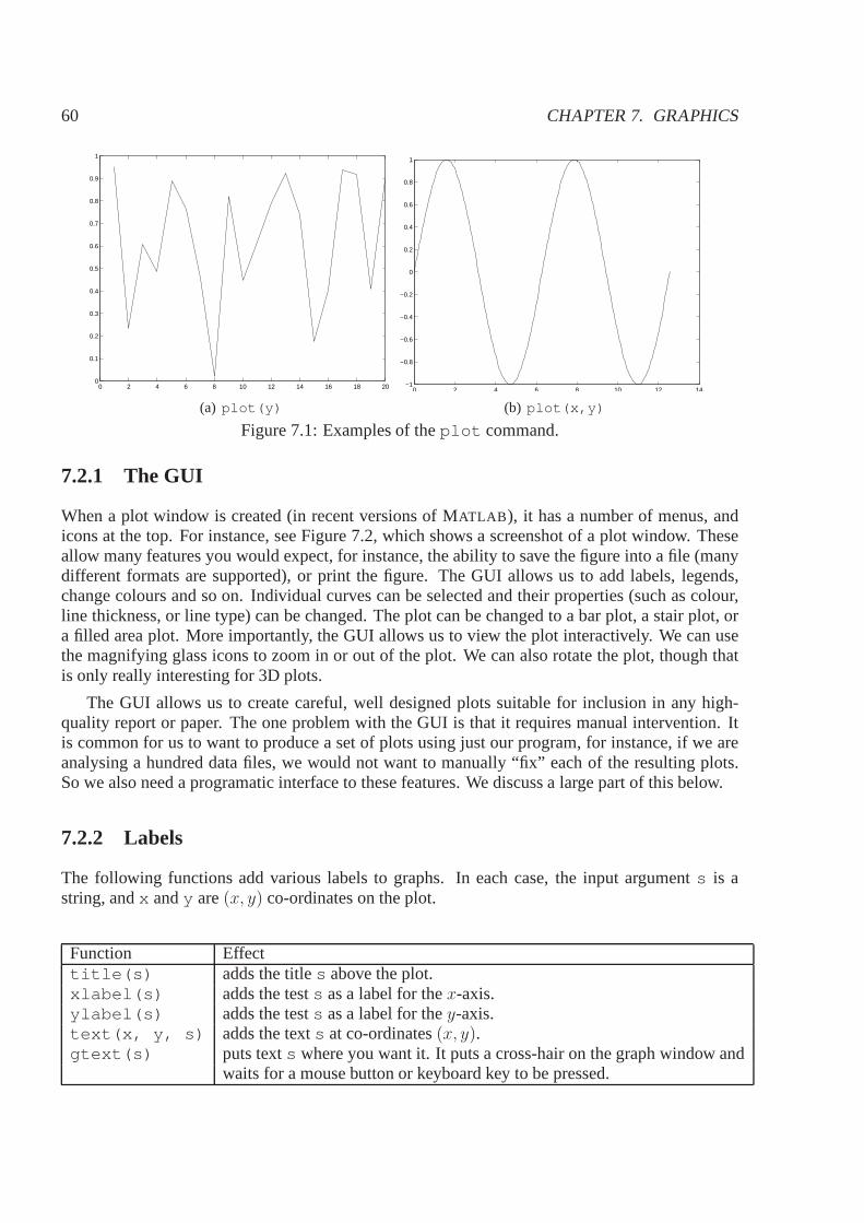
60 CHAPTER 7. GRAPHICS
0 2 4 6 8 10 12 14 16 18 200
0.1
0.2
0.3
0.4
0.5
0.6
0.7
0.8
0.9
1
(a) plot(y)
0 2 4 6 8 10 12 14−1
−0.8
−0.6
−0.4
−0.2
0
0.2
0.4
0.6
0.8
1
(b) plot(x,y)
Figure 7.1: Examples of theplot command.
7.2.1 The GUI
When a plot window is created (in recent versions of MATLAB ), it has a number of menus, andicons at the top. For instance, see Figure 7.2, which shows a screenshot of a plot window. Theseallow many features you would expect, for instance, the ability to save the figure into a file (manydifferent formats are supported), or print the figure. The GUI allows us to add labels, legends,change colours and so on. Individual curves can be selected and their properties (such as colour,line thickness, or line type) can be changed. The plot can be changed to a bar plot, a stair plot, ora filled area plot. More importantly, the GUI allows us to viewthe plot interactively. We can usethe magnifying glass icons to zoom in or out of the plot. We canalso rotate the plot, though thatis only really interesting for 3D plots.
The GUI allows us to create careful, well designed plots suitable for inclusion in any high-quality report or paper. The one problem with the GUI is that it requires manual intervention. Itis common for us to want to produce a set of plots using just ourprogram, for instance, if we areanalysing a hundred data files, we would not want to manually “fix” each of the resulting plots.So we also need a programatic interface to these features. Wediscuss a large part of this below.
7.2.2 Labels
The following functions add various labels to graphs. In each case, the input arguments is astring, andx andy are(x, y) co-ordinates on the plot.
Function Effecttitle(s) adds the titles above the plot.xlabel(s) adds the tests as a label for thex-axis.ylabel(s) adds the tests as a label for they-axis.text(x, y, s) adds the texts at co-ordinates(x, y).gtext(s) puts texts where you want it. It puts a cross-hair on the graph window and
waits for a mouse button or keyboard key to be pressed.

7.2. DECORATING THE FIGURE 61
Figure 7.2: Example of a plot window.
The size of the “font” used in labels can be controlled by setting options. For exampletext ,title , xlabel , ylabel , andlegend allow optional arguments of the form’fontsize’followed by an integer. The color can be changed using the’color’ option just as for a plotcommand (see below). Labels can also include a limited subset of LaTeX commands for mathe-matical symbols. LaTeX can be used to create greek symbols, superscripts and subscripts and asmall set of other mathematical constructions useful in some labels. For instance, the followingcommands, produce the graph shown in Figure 7.3.
x = 0 : pi/40 : 4 * pi;y = sin(x);plot(x, y);title( ’Titles appear above the graph’, ’fontsize’, 20)xlabel( ’instead of writing phi we write \phi’ )ylabel( ’ylabels are presented vertically’ )text(9.3, 0.2, ’a sin curve’)

62 CHAPTER 7. GRAPHICS
0 2 4 6 8 10 12 14−1
−0.8
−0.6
−0.4
−0.2
0
0.2
0.4
0.6
0.8
1Titles appear above the graph
instead of writing phi we write φ
ylab
els
are
pres
ente
d ve
rtic
ally
a sin curve
Figure 7.3: Examples of various labelling command.
7.2.3 Other graph features
There are many other ways we can control the general appearance of our plot, for instance:
Function Effectaxis([xmin xmax ymin ymax]) changes thex andy range of the axesaxis auto returns axes to autoscalingaxis tight makes the axes scaling fit the data tightlyaxis ij puts the axis in “matrix” mode where the y values are reversedaxis xy puts the axis in the default Cartesian modeaxis square makes the current axes squareaxis normal makes the current axes fit the plot windowaxis off turns off all axis labellingaxis on turn axis labelling back ongrid adds/removes grid lines to/from the current graph.xlim([xmin xmax]) change the range of thex axisylim([ymin ymax]) change the range of they axis
7.2.4 Line types, plot symbols and colour
Line types, and plot symbols, and the line colour may all be set when we create a plot. There aretwo approaches, firstly, there is an optional input argumentto theplot function that can contain

7.2. DECORATING THE FIGURE 63
a series of “flags” which each indicate something about the resulting plot.
Colour Marker Line TypeFlag Colour Flag Marker Flag Line Type
b blue . point - solidg green o circle : dottedr red x x-mark -. dashdotc cyan + plus -- dashed
m magenta * stary yellow s squarek black d diamondw white v triangle (down)
ˆ triangle (up)< triangle (left)> triangle (right)p pentagramh hexagram
By combining three (or fewer) of these flags, we construct a particular plot, e.g.,
plot(x,y, ’--’)
plotsy againstx and joins the points with a dashed line whereas
plot(x,y, ’o’)
draws circles at the data points with no lines joining them. Combinations are valid, e.g.,
plot(x,y, ’--mo’)
plots a magenta dashed line, with circles at the data points.
The second approach to setting plot characteristics is to include a series of pairs of optionalarguments to the plot command, for instance,
plot(x,y, ’color’, ’m’, ’linestyle’, ’--’, ’marker’, ’o’)
which would draw a plot in the colour magenta, with dashed lines between each point, and the datapoints themselves shown by ’o’. A brief list of such arguments is shown in the following table:
Option name Valid values Default Effectcolor b,g,r,m,c,y,k,w or a[r, g, b]-color b sets line and marker colourlinestyle ’-’, ’–’, ’:’, ’-.’ ’-’ sets the line stylemarker see table above none sets the marker at data pointslinewidth positive integers 1 sets the width of linesmarkersize positive integers 6 sets the size of markers
Note the American spelling of color. There are many other options for plots (for instance we canchange the colour of the inside and edge of a marker independently). Seehelp plot for moredetails.

64 CHAPTER 7. GRAPHICS
7.2.5 Fonts
The font refers to the style of writing used. Typically, the main thing we might change abouta font would be the size. As noted earlier, several commands (e.g. text , title , xlabel ,ylabel , legend ) allow optional arguments of the form’fontsize’ followed by an integer.For instance we might write:
title(’This is the BIG title’, ’fontsize’, 24);
which would place a title on the plot in a large font. The colorcan also be change using the’color’ option just as for a plot command (see above). A list of commonoptions for fonts isincluded below
Option name Valid values Default Effectcolor b,g,r,m,c,y,k,w or a[r, g, b]-color k sets font colourfontsize positive integer 10 text size in “points”fontangle normal, italic or oblique normal style of fontfontweight light, normal, demi or bold normal style of fontrotation an angle in degrees 0 rotate the text by the angle
More options can be found in the MATLAB documentation.
However, this will not change the size of text used for numbers on axes. To do so, we need tochange the properties of the current set of axes, which we cando using the command:
set(gca, ’fontsize’, 24);
For instance see the results shown in Figure 7.6 where this command has been used to make thelog axes more readable. The input argumentgca is a variable that MATLAB uses to refer to thecurrent set of axes. In fact,set(gca, ...) can be used to change many properties of the axes,including where labels appear, and what labels are used. Another common use is to change thethickness of the lines used, e.g. by typing
set(gca, ’linewidth’, 3);
but general use ofset is beyond the scope of this course, and we will not cover it in more detailhere.
One final note: although MATLAB is usually case sensitive, the options used above aren’t, i.e.,’FontSize’ is the same as ’fontsize’.
7.3 Multiple plots
7.3.1 More than one figure
It is common for us to want to see more than one plot at a time. MATLAB allows this through thefigure function. By itself,figure will create a new window, ready for a new plot. If we usefigure(n) , where it has an integer argument, it will either switch to windown, or create a newwindown if one doesn’t exist. For example, we might type something like

7.3. MULTIPLE PLOTS 65
x = 0: pi/100: pi;y = cos(x);z = sin(x);figure(1); % create figure window 1plot(x,y); % plot (x,y) in window 1figure(2); % create figure window 2plot(x,z); % plot (x,z) in window 2
figure(1); % swap back to window 1ylabel(’y’); % set the y-axis label on window 1figure(2); % swap back to window 2ylabel(’z’); % set the y-axis label on window 2
This series of commands will result in two figure windows, plotting x versus y and z, with theappropriate y-axis labels.
7.3.2 Multiple subplots
Sometimes we want to do multiple plots, but we wish them to appear as subplots on a singlewindow. We can do this using thesubplot function. The command takes three input arguments,the first two specify how many rows and columns of subplots should appear. The third specifieswhich plot to use. For instance, we could take the two plots from the previous example, and placethem in the same window using the following statements.
x = 0: pi/100: pi;y = cos(x);z = sin(x);figure(1); % create figure window 1subplot(2,1,1) % create two subplots, one above the other, a nd
% use the first one for the next plotplot(x,y);subplot(2,1,2) % use the second subplot for the next plotplot(x,z);
Figure 7.4(a) shows the result.
7.3.3 Multiple plots on the same graph
It is sometimes preferable to put two plots onto the same graph so that they can be directly com-pared. We can do this using thehold command. By default, if we call plot twice, the old plotwill be removed and replaced by the new one. However, if we call
hold on
the new plot will be overlaid on the old plot. The commandhold off reverts back to the defaultbehaviour. For instance, repeating the above example:
x = 0: pi/100: pi;

66 CHAPTER 7. GRAPHICS
0 0.5 1 1.5 2 2.5 3 3.5−1
−0.5
0
0.5
1
0 0.5 1 1.5 2 2.5 3 3.50
0.2
0.4
0.6
0.8
1
(a) Two subplots.
0 0.5 1 1.5 2 2.5 3 3.5−1
−0.8
−0.6
−0.4
−0.2
0
0.2
0.4
0.6
0.8
1
cossin
(b) Two plots on the same graph.
Figure 7.4: Examples plotting multiple curves.
y = cos(x);z = sin(x);figure(1); % create figure window 1hold off % remove any old plots on the figureplot(x,y, ’-’); % do the first plothold on % allow us to add an extra plotplot(x,z, ’--’);% add a second plot, with a different line st ylelegend(’cos’, ’sin’);
The final command above is for creating a legend for the plots.In its simple form, as illustratedabove, we simply calllegend with a a list of string inputs, and these are assigned to the differentplots. Figure 7.4(b) shows the result. Note however, thatlegend has many options.
7.3.4 Plotting a matrix
A faster approach to putting multiple plots onto a single graph is to plot a matrix (rather than avector). MATLAB will then produce (by default) one curve for each column of the matrix usingdifferent colours for each line. For instance if we used the following code
x = [0: pi/40 : 2 * pi]’;Y = [cos(x) sin(x)];plot(Y);
we would plot both the sine and cosine curves on the same graphin different colours. We can usethe correctx axis using a command like
x = [0: pi/40 : 2 * pi]’;Y = [cos(x) sin(x)];plot(x, Y);
and we will get a graph such as shown in Figure 7.5(a) (though in colour). We can make thismore general by turning bothx andy co-ordinates in the plot into matrices. A simple example ofthe practicality of this approach is in plotting confidence intervals around data points, e.g., for thepurpose of demonstration use random values as follows:
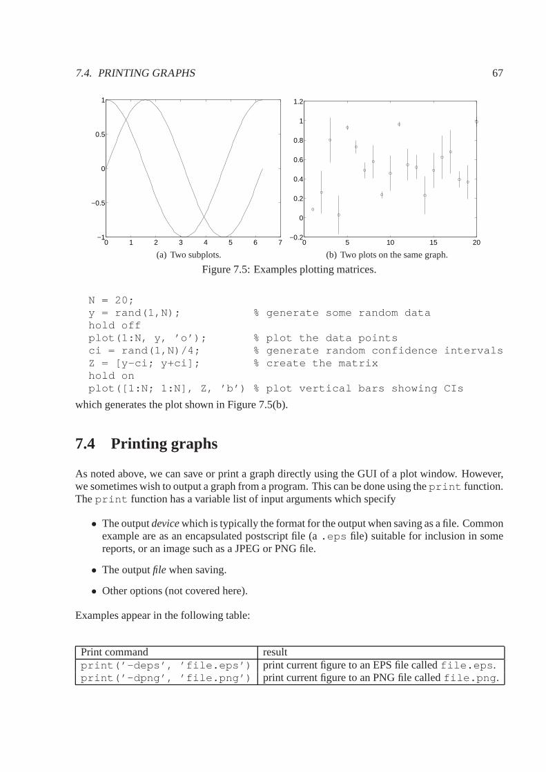
7.4. PRINTING GRAPHS 67
0 1 2 3 4 5 6 7−1
−0.5
0
0.5
1
(a) Two subplots.
0 5 10 15 20−0.2
0
0.2
0.4
0.6
0.8
1
1.2
(b) Two plots on the same graph.
Figure 7.5: Examples plotting matrices.
N = 20;y = rand(1,N); % generate some random datahold offplot(1:N, y, ’o’); % plot the data pointsci = rand(1,N)/4; % generate random confidence intervalsZ = [y-ci; y+ci]; % create the matrixhold onplot([1:N; 1:N], Z, ’b’) % plot vertical bars showing CIs
which generates the plot shown in Figure 7.5(b).
7.4 Printing graphs
As noted above, we can save or print a graph directly using theGUI of a plot window. However,we sometimes wish to output a graph from a program. This can bedone using theprint function.Theprint function has a variable list of input arguments which specify
• The outputdevicewhich is typically the format for the output when saving as a file. Commonexample are as an encapsulated postscript file (a.eps file) suitable for inclusion in somereports, or an image such as a JPEG or PNG file.
• The outputfile when saving.
• Other options (not covered here).
Examples appear in the following table:
Print command resultprint(’-deps’, ’file.eps’) print current figure to an EPS file calledfile.eps .print(’-dpng’, ’file.png’) print current figure to an PNG file calledfile.png .

68 CHAPTER 7. GRAPHICS
There are many other options, file formats, and ways of calling print . Usehelp print formore details
The size of the output graph can be controlled by setting parameters of the current figurewindow, which MATLAB refers to asgcf . For example
set(gcf,’PaperUnits’,’centimeters’,’PaperPosition’, [0 0 10 12]);
would make the figure10 × 12 centimeters in size. There are other properties of a figure that canbe changed to in turn change the output from theprint function.
7.5 Colours
MATLAB allows use of colours in plots. There are several ways to do so. The simplest is to usethe one character codes given above, with their direct association to a colour. However, somecommands do not take such codes, and at other times we wish to use different colours.
There are several approaches, but the most general is to specify a colour as a RGB triple. Thatis, we give thered, green andblue component of the colour in a 3 element vector. Many colourscan be expressed in this way, for instance, the common MATLAB colours are shown below:
Color code Color Red Green Blueb blue 0 0 1g green 0 1 0r red 1 0 0c cyan 0 1 1
m magenta 1 0 1y yellow 1 1 0k black 0 0 0w white 1 1 1
A value of 1 (say for the red component) would mean that component is as strong as possible,whereas a value of zero means it is not present at all.
More about RGB colours can be found, for instance, athttp://en.wikipedia.org/wiki/RGB . Example colours can be found athttp://www.pitt.edu/ ˜ nisg/cis/web/cgi/rgb.html , though note that commonly the RGB values are specified from 0to 255. Toconvert to MATLAB values, divide by 255.
An alternative approach to colors sometimes used in MATLAB is to create acolormap . Thecolormap maps a set of integers to a RGB triple. It is represented by aN × 3 matrix, where eachrow is a RGB triple. An integern is then mapped to the colour of thenth row of the table. Someplotting commands, such assurf and image (which we will see later) automatically use thecurrent colormap. MATLAB has a set of predefined color maps that can be used via thecolormapfunction. For instancecolormap(’default’) uses the standard MATLAB colormap, andcolormap(’gray’) uses a grayscale (B&W) colormap. MATLAB has a number of built inexamples that demonstrate the power of these color maps, e.g., try
load spine
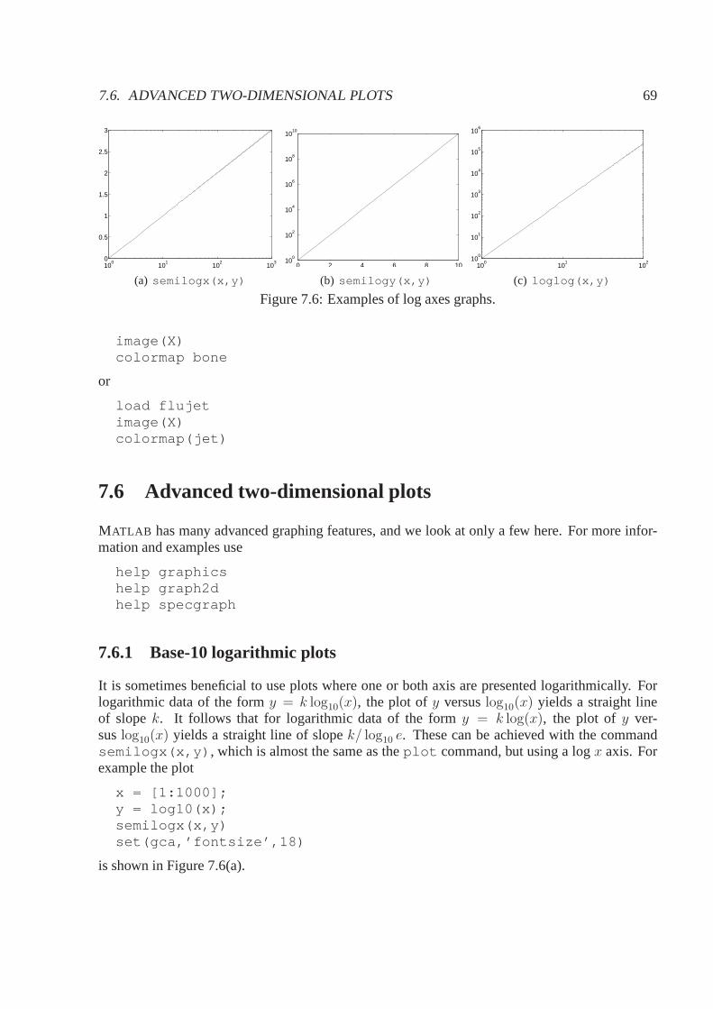
7.6. ADVANCED TWO-DIMENSIONAL PLOTS 69
100
101
102
103
0
0.5
1
1.5
2
2.5
3
(a) semilogx(x,y)
0 2 4 6 8 1010
0
102
104
106
108
1010
(b) semilogy(x,y)
100
101
102
100
101
102
103
104
105
106
(c) loglog(x,y)
Figure 7.6: Examples of log axes graphs.
image(X)colormap bone
or
load flujetimage(X)colormap(jet)
7.6 Advanced two-dimensional plots
MATLAB has many advanced graphing features, and we look at only a fewhere. For more infor-mation and examples use
help graphicshelp graph2dhelp specgraph
7.6.1 Base-10 logarithmic plots
It is sometimes beneficial to use plots where one or both axis are presented logarithmically. Forlogarithmic data of the formy = k log10(x), the plot ofy versuslog10(x) yields a straight lineof slopek. It follows that for logarithmic data of the formy = k log(x), the plot of y ver-suslog10(x) yields a straight line of slopek/ log10 e. These can be achieved with the commandsemilogx(x,y) , which is almost the same as theplot command, but using a logx axis. Forexample the plot
x = [1:1000];y = log10(x);semilogx(x,y)set(gca,’fontsize’,18)
is shown in Figure 7.6(a).

70 CHAPTER 7. GRAPHICS
For exponential data of the formy = 10kx, the plot oflog10(y) versusx yields a straight line ofslopek. (This is sincelog10(y) = kx and a plot ofkx versusx is a straight line of slopek.) Itfollows that for exponential data of the formy = ekx, the plot oflog10(y) versusx yields a straightline of slopek log10 e. These can be achieved with the commandsemilogy(x,y) , e.g.,
x = [0:10];y = 10 .ˆ x;semilogy(x,y)set(gca,’fontsize’,18)
(results shown in Figure 7.6(b)) and
x = [0:10];y = exp(x);semilogy(x,y)set(gca,’fontsize’,18)
For data of the formy = xk, a plot of log10(y) versuslog10(x) yields a straight line of slopek.(This is sincelog10(y) = k log10(x) and a plot ofk log10(x) versuslog10(x) is a straight line ofslopek.) This can be achieved with the commandloglog(x,y) . For example Figure 7.6(c)shows the results of
x = [0:100];y = x.ˆ2.7;loglog(x,y)set(gca,’fontsize’,18)
It is useful to note that if we use thehold on command to put more than one plot onto agraph, the first plot determines the type of axes. So if we specify loglog first, then even ifsubsequent commands useplot , all graphs will appear on with the same log-log axes.
7.6.2 Histograms
There is a simple approach to producing a histogram in MATLAB . In is simplest form, we simplycall hist(data) , however, we often want to specify the exact bins being used,or at least theirnumber and we can do so through an optional second argument. For instance:
data = randn(1000,3); % generate random "Normal" datahist(data, 30); % do a histogram with 30 binsset(gca,’fontsize’,18)
Following these commands, MATLAB will automatically scale the bins to include all of the data,and then generate a figure, as shown in Figure 7.7(a).
When the input data is a matrix (rather than a vector) the histogram will show multiple barsfor each column of the data.
MATLAB also allows us to put the result of the histogram command intoan output vector,rather than a figure, which we can then plot using the various plotting commands we have alreadyseen. If we want to do a histogram plot, though, we can so usingthebar command, which drawsa bar plot of a set of data. For instance,

7.6. ADVANCED TWO-DIMENSIONAL PLOTS 71
−4 −2 0 2 40
10
20
30
40
50
60
70
80
90
(a) hist(data, 30)
−4 −2 0 2 40
20
40
60
80
100
120
140
160
180
(b) bar(x, y)
Figure 7.7: Examples of histograms and bar charts.
data = randn(1000,3); % generate a matrix of data[y,x] = hist(data, 20); % do a histogram with 30 bins, but don’ t plotbar(x, y);set(gca,’fontsize’,18)
the results of which are shown in Figure 7.7(b).
7.6.3 Thefill function
The fill function allows us to fill in a polygonal area with a particular colour. The command isexecuted as follows:
fill(x, y, colour)
wherex andy vectors specify thex andy co-ordinates of the vertexes of the polygon, and colourspecifies the fill colour in one of the formats above (either a letter code or a RGB triple).
An example of the fill command appears below. The code below draws a rainbow. The codeconstructs an (approximate) elliptical arc for the outsideand inside of each “bow” of the rainbow(i.e. for each colour). The code then puts the outer and innerarc together to approximate a circulararc which it then fills with the correct color (specified in thearraycolors ).
% draw a rainbowN = 50;step = 0.07;r = 1:-step:1-7 * step;theta = 0:pi/N:pi;alpha = 1.4;colors = [[1 0 0]; % red
[1 0.5 0]; % orange[1 1 0]; % yellow[0 1 0]; % green

72 CHAPTER 7. GRAPHICS
[0 0 1]; % blue[0.3 0 0.4]; % indigo[0.2 0 0.3]; % violet
];figure(1)hold offplot(0,0)hold onfor i=1:length(r)-1
x1 = alpha * r(i) * cos(theta);y1 = r(i) * sin(theta);x2 = alpha * r(i+1) * cos(fliplr(theta));y2 = r(i+1) * sin(fliplr(theta));
x = [x1 x2];y = [y1 y2];
% plot(x, y, ’.’);fill(x, y, colors(i,:));
endaxis equal % make the scales on the two axes equalaxis tight % fit the axes tightly around the plot
The output of which is shown in Figure 7.8.
−1 −0.5 0 0.5 10
0.2
0.4
0.6
0.8
1
Figure 7.8: Output of rainbow.m.
7.6.4 Images
Displaying images is simple, but there are several details to get right. Firstly, there are two mainrepresentations of an image. We can represent it as an array of numbers that are mapped to colorsvia a colormap, or as an 3D array where two dimensions represent the 2 spatial dimensions of animage, and the third allows us to store the components of the colours (for instance the RGB triple).When creating or reading an image, it is important to understand what format it will be in. Seedocumentation forimread to learn more.

7.6. ADVANCED TWO-DIMENSIONAL PLOTS 73
The main command for displaying an image is the creatively nameimage(C) function. IfC isaM×N matrix, the values will be mapped to colors in the display using the current colormap (seeSection 7.5). If the colormap is subsequently changed, thenthe image will change colours. Thefunctionimagesc scales the values ofC to the potential range of the colormap before displaying.
If C is aM × N × 3 array, then it will be displayed interpreting each of the triples as RGBcolours, i.e.,C(:,:,1) , C(:,:,2) and C(:,:,3) are interpreted as red, green and blueintensities, respectively. The colormap is ignored. The range of values forC depends on its type.For a standarddouble array, the range is[0, 1], but if the array uses an integer type such asuint8 the range is[0, 255]. Care must be taken when importing data that the type is correct.
We create a simple example below
N = 250; M = 250; alpha = 0.001;x = 1:N;y = 1:M;[X,Y] = meshgrid(x,y);C = exp( -alpha * ((X-N/2).ˆ2 + (Y-M/2).ˆ2) );colormap(’gray’); % change the colormap to B&Wimage(255 * C); % show the image using the colormapaxis image; % make the axes look right
% create a RGB imageC(:,:,1) = exp( -alpha * ((X-N/2).ˆ2 + (Y-M/2).ˆ2) );C(:,:,2) = exp( -alpha * ((X-N/2).ˆ2 + (Y-M/2).ˆ2) );C(:,:,3) = exp( -alpha * ((X-N/2).ˆ2 + (Y-M/2).ˆ2) );image(C);axis image;
7.6.5 Others
There are many other MATLAB functions for drawing plots:
• plotyy : Sometimes we wish to plot two curves with different scales on the same plot.plotyy does this with one axis on the left, and the other on the right.
• pie : allows us to draw a pie chart.
• polar : draw a plot of polar co-ordinate data.
• stem : does a “stem” plot, showing lines growing from thex axis with a marker at thetop. Often used in discrete signal processing, along with stairstep plots, which we can drawwithstairs .
• contour : allows one to draw a contour plot of some set of data. For example, if a matrixZ represented heights, then a contour plots would show curvesof constant height.
• quiver : allows plots of a vector field. There are many other volume and vector visualiza-tion functions.

74 CHAPTER 7. GRAPHICS
• movie in conjunction withgetframe can be used to create animations that can then besaved as movies.
There are many others: rose plots, waterfall plots, Voronoidiagrams, Pareto charts, comet chartsand so on. However, rather than considering each, we shall goon to consider another large groupof plots, those in 3D.
7.7 Three-dimensional plots
MATLAB has a number of functions for displaying and visualising data in three dimensions. Thefunctionplot3 is the 3-D version ofplot , which is called in the following form:
plot3( x, y, z )
wherex , y andz are (typically) vectors specifying the(x, y, z) co-ordinates of a series of points.This command draws a picture of the 3-D curve through the points whose coordinates are theelements of the vectorsx , y andz . As an example
z = 0 : pi/50 : 10 * pi;x = exp(-0.02 * z) . * sin(z);y = exp(-0.02 * z) . * cos(z);plot3( x, y, z);xlabel(’x-axis’);ylabel(’y-axis’);zlabel(’z-axis’);
produces the inwardly-spiralling helix shown in figure 7.9.Theplot3 command admits the sametypes of options as the 2Dplot command, so we can set line colour and style, the marker types,and linewidth. We can also control the axes as before, and even place text on the graph usinglabels, or the text command called with four input parameters, e.g.,
text(x,y,z, ’text we wish to write’);
The figure’s GUI also allows the same types of options as before, but there is an additionaluseful button for 3D plots. The image displayed is really a 2Dprojection of the 3D curve we wish
to examine. The rotate button allows us to use the mouse to rotate the projection that we seeso that we can examine the curve from different perspectives. The viewpoint can be changed inthe program using theview function.
7.7.1 Mesh surfaces
Another standard activity in 3D is to plot a representation of a surface. For instance, imagine wewished to plot the function:
f(x, y) = 5y − x2
over the range−4 ≤ x ≤ 4 and0 ≤ y ≤ 5. The simple approach to plotting such a function is tocalculate it at a set of sample points, and plot an approximation of the surface at these points usingthemesh command.
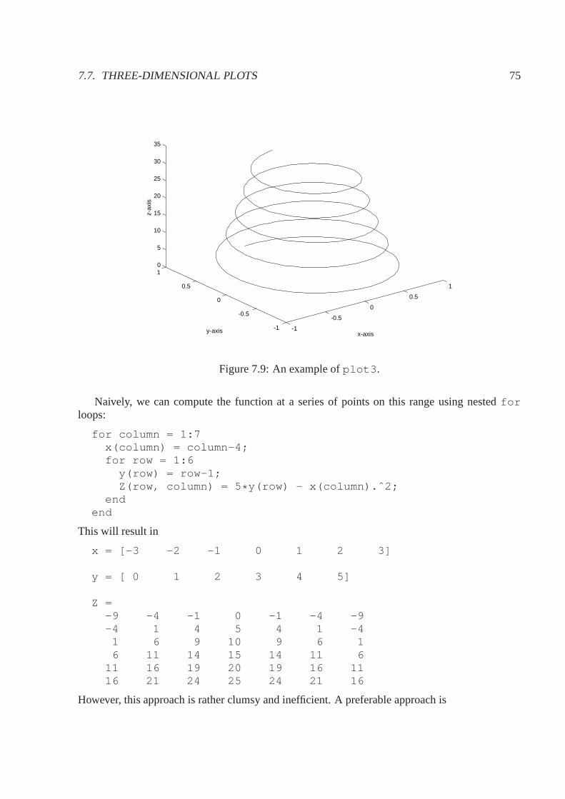
7.7. THREE-DIMENSIONAL PLOTS 75
-1
-0.5
0
0.5
1
-1
-0.5
0
0.5
10
5
10
15
20
25
30
35
x-axisy-axis
z-ax
is
Figure 7.9: An example ofplot3 .
Naively, we can compute the function at a series of points on this range using nestedforloops:
for column = 1:7x(column) = column-4;for row = 1:6
y(row) = row-1;Z(row, column) = 5 * y(row) - x(column).ˆ2;
endend
This will result in
x = [-3 -2 -1 0 1 2 3]
y = [ 0 1 2 3 4 5]
Z =-9 -4 -1 0 -1 -4 -9-4 1 4 5 4 1 -4
1 6 9 10 9 6 16 11 14 15 14 11 6
11 16 19 20 19 16 1116 21 24 25 24 21 16
However, this approach is rather clumsy and inefficient. A preferable approach is

76 CHAPTER 7. GRAPHICS
step = 1;x = -3:step:3;y = 0:step:5;[X,Y] = meshgrid(x,y);Z = 5* Y - X.ˆ2;
which produces the same vectorsx andy , and matrixZ. It also creates the matrixX with the rowsequal to the vectorx , and matrixY with columns equal to the vectory . This approach has theadvantages that it is more efficient (faster), and also allows us to change thestep parameter toplot more, or fewer points as needed. The statements
mesh(X, Y, Z);set(gca,’fontsize’, 24);xlabel(’x’);ylabel(’y’);
then plots the surfaceZ as a “wire frame”, where the matrices provide the(x, y, z) co-ordinates onthe surface we wish to plot. In our case, because we have a regular grid, we might also have calledmesh(x,y,Z) . In each case, we might imagine the valuesZ as heights on a map of terrain ateach(x, y) co-ordinate. The plot produced by these commands in shown inFigure 7.10(a). Notethat by default MATLAB will use colours from the current colormap to highlight changes in value(i.e., the range of values ofZ will be scaled and mapped to the colormap and these colors will beused to change the mesh).
An alternative to a mesh surface is to fill in the rectangles between points using thesurffunction. For instance, the above surface can be displayed as in Figure 7.10(b) using
surf(x, y, Z);set(gca,’fontsize’, 24);xlabel(’x’);ylabel(’y’);
Again MATLAB uses colours from the current colormap to highlight changesin value. The“faceted” view shown by default insurf can be smoothed by changing theshading mode ofthe plot. The default isfaceted interpolation, but we can also useflat to get rid of the meshlines, orinterp to make the shading color smooth so that we see an apparently smooth surface.Figures 7.10(c) and 7.10(d) show the results of the following commands:
surf(x, y, Z); shading flat;surf(x, y, Z); shading interp;
More information on 3D plots can be found from the individualhelp for each function, andfrom help graph3d .

7.7. THREE-DIMENSIONAL PLOTS 77
−50
5
0
5−20
0
20
40
xy
(a) mesh(x,y,Z)
−50
5
0
5−20
0
20
40
xy
(b) surf(x,y,Z)
−50
5
0
5−20
0
20
40
(c) surf(x,y,Z); shading flat;
−50
5
0
5−20
0
20
40
(d) surf(x,y,Z); shading interp;
Figure 7.10: Examples of surface and mesh plots.

78 CHAPTER 7. GRAPHICS

Chapter 8
Defining Functions with M-files
As we have seen, MATLAB has many built in functions. However, it is common for us to wish tocreate our own functions. This allows us to encapsulate a group of MATLAB statements. Encapsu-lation improves code re-usability, by enabling us and others to reuse the same function more thanonce without retyping the same code. It improves code maintainability by allowing us to fix a bugin one place (in the function) rather than in all of the placeswe might have used that function.
We call thismodularityin programming. It separates the internal logic of a function from theinterface— the inputs and outputs of the function. Modularity is particularly important for largesoftware systems, where more than one programmer may be working on the system. It allows thetwo programmers to work on separate code without knowing thedetails, except for the functioninterfaces. Other programming languages provide modularity in various ways (e.g. subroutines,procedures, etc.), but MATLAB ’s primary approach is to allow us to define our own functions.
Another reason to use functions in MATLAB is that they will often run faster than the equivalentscript file.
8.1 Some examples
We will start with a couple of illustrative examples of function definitions. As when creating script.m files, we will use MATLAB ’s editor to input the commands into a file.
8.1.1 Harmonic oscillators
If two coupled harmonic oscillators are considered as a single system, the output of the system asa function of timet could be something like
h(t) = cos(8t) + cos(9t).
We can create a function.m file calledharmonic.m with the following two lines
function h = harmonic(t)h = cos(8 * t) + cos(9 * t);
79

80 CHAPTER 8. DEFINING FUNCTIONS WITH M-FILES
Then we can then call the function in another piece of MATLAB code, for instance at the MATLAB prompt,just as we do for other functions, e.g.,
x = pi/2;y = harmonic(x);
Note the following:
1. The name of the function — what we type when we want to call it— is defined on the firstline of the file by the statementfunction y = harmonic(t) . The filename of the.mfile must match this name, for instance in this case we save thefile asharmonic.m .
2. The variablet in the functionharmonic.m is the input variable. It implicitly creates avariable calledt inside the function. The variable will be initialized with the value of thecorresponding input variable in the function call. In this example, it will start with the valuepi/2 , obtained from the variablex . Note that if we changet inside the function, it has noeffect onx . The input serves only to set the initial value oft and thereafter the connectionbetweenx andt is broken.
3. The variableh in the function file is theoutput variable. We must assign a value toh atsome point in our function.m file. The value we assign will be passed out to the outputvariable when we call the function. For instance in the example, the value ofh inside thefunction will be assigned to the variabley , after the function is finished.
4. It is good coding practice to always use semi-colons at theend of lines in MATLAB functionsso that the function has no unintended “side-effects” such as printing out intermediate val-ues. However, we may ignore this guideline during debuggingof a function.
5. We don’t have to use a variable as input to a function, we could also use an expression, oranother function. We can also pass vectors and matrices as inputs, for instance
y = harmonic([0:pi/40:6 * pi]);plot([0:pi/40:6 * pi], y);
We sometimes talk ofinput argumentsinstead of input variables. They are the same thing (likewisefor output arguments).
8.1.2 Statistics
Consider the following more general example which calculates the mean and the standard devia-tion of the values in the vectorx . We’ll save this function in a file calledstats.m .
function [average, standard_deviation] = stats(x)% Calculates the mean and standard deviation of% the data in the vector x.average = mean(x);standard_deviation = std(x);
We can now test it with some random numbers:

8.2. THE BASIC RULES FOR FUNCTION FILES 81
r = rand(100,1);[ave,st_dev] = stats(r)
The function will calculate the mean and standard deviationof the input (random) numbers, andwill pass these to the output variablesave andst_dev .
8.2 The basic rules for function files
A function M-file name.m has the following general form.
function [out1, out2,... ,outN] = name(inp1, inp2,... ,inp M)% comments to be displayed by helpstatementsout1 = expression1;out2 = expression2;...
where... is used here to indicate that there may be an indefinite numberof input and outputvariables (you would not type this). The function would typically be called by typing
[o1, o2, ... , oN] = name(i1, i2, ... ,iM);
The rules that wemustfollow when defining a function are as follows:
1. The function name and the name of the file containing it mustbe identical except for the.m filename extension. Remember MATLAB is case sensitive. It is suggested that you uselower-case for function names as this will increase portability of your code to other operatingsystems.
2. The function name must follow MATLAB ’s rules for variable names, as must the input andoutput variables.
3. The function file must start with the reserved wordfunction , followed by a vector of theoutputs, and equals sign, the name of the function, and roundbrackets with a list of inputvariables.
4. If there is only one output variable square brackets are not necessary (even if it is a vector).If there is more than one output variable, the output variables must be separated by commasand enclosed in square brackets (as with a vector). This is true both in the function definition,and when we call a function.
5. If an output is unassigned, this may cause an error, so we need to have at least one statementassigning values to each output variable. Often these statements are at the end of a functionfile. They don’t have to be, but it can improve program readability to place them there.
6. Note that if the function changes the value of any of its input variables the change does notaffect the corresponding variable used in the call to the function.

82 CHAPTER 8. DEFINING FUNCTIONS WITH M-FILES
8.2.1 Optional inputs and output
We don’t need to call a function with all of its inputs and output variables. The input variables thatare not assigned will be undefined until they are given a valuein the program, as will unassignedoutputs. For instance, we could call
r = rand(100,1);ave = stats(r);
This code would assign the variableave the value of the internal output variableaverage , butthe output variablestandard_deviation is not assigned to any workspace variable.
Likewise, we can define a functionadd_them_up that adds two numbers, when we inputtwo, or just outputs the original value when we only use one input as follows. It uses the functionexist to test whether the second variable exists and reacts appropriately.
function result = add_them_up(x,y)if (exist(’y’,’var’))
result = x+y;else
result = x;end
We can now call this function two different ways
add_them_up(1, 3)add_them_up(4)
and in both cases it will output the value 4.
This type of construction allows us to have optional inputs to a function, with default argumentswhen an input is not used. It is somewhat limited, because it is dependent on order. We can’t omitinput parameterN , but includeN+1. A better approach might be to use an input variable structure,but this is outside the scope of this course.
The above mechanism is also quite clumsy when the number of inputs is large. To aid in thisMATLAB automatically creates two extra variables when a function is called:
Variable Meaningnargin The number of input variables for this function call.nargout The number of output variables for this function call
We could use these in the above example be rewriting the function as follows:
function result = add_them_up(x,y)if (nargin == 2)
result = x+y;else
result = x;end

8.2. THE BASIC RULES FOR FUNCTION FILES 83
An even more flexible mechanism is to usevarargin or varargout in place of all orpart of the list of input arguments. This allows us to specifyexplicitly that we don’t know thenumber of input or output arguments. This type of mechanism is used in functions such asplotto allow us to specify an arbitrary number of options to the command, or infprintf to allow usto provide an arbitrarily long list of variables to substitute into the format string. We will no gofurther into this type of construction here, but it is important to realize that such facilities exist.
8.2.2 Scope
The input variables (inp1 , inp2 , ...) and output variables (out1 , out2 , ...) are the function’smeans of communicating with the workspace. The input variables allow you to pass in valuesto the function, and the output variables allow values to be passed out. There can be some otherinteractions, for instance if the function reads a file, or presents at plot, but typically these do notpass values in or out of the workspace.
Variables defined inside a MATLAB function havelocal scope. This means that they cannot beseen outside of this function. We cannot obtain their values, or interact with these variables in anyway. For instance, they will not appear in the workspace. Even the implicitly created input andoutput variables cannot be accessed outside the function except at the start (for input variables)and the finish (for output variables).
There are various reasons for this. Firstly, it is highly desirable to minimize the side-effects offunctions. This makes program behaviour more predictable.Side-effects can have unanticipatedconsequences!
Secondly, giving function variables local scope improves the modularity of code. It simplifiesthe interface between the function and other programs. It makes the interface as simple as callingthe function, e.g.
[ave,st_dev] = stats(r)The result is that MATLAB functions are easy to use without necessarily examining allof theMATLAB code in the function. We just need to look at the first line of the function to see how tocall it. In essence, we can treat a MATLAB function as a black-box that performs an action, andwe don’t need to understand how it does it.
The third important result of local scope is that we avoidname collisionsbetween variablesinside and outside the function. Say I want to use a complex function defined by third party. Itmay define many internal variables. I don’t want to have to make sure all of my variables havedifferent names. For instance, they may use the common namex inside their code, and I maywant to usex for something different outside of the code. I don’t want to have to check that willbe OK. This problem may sound trivial, but imagine I am calling a hundred different functionseach with its own variable names. If there was overlap in the namespaces, then not only mightmy names collide with the functions’ variable names, but also the functions might have collisionsbetween each others variables. Local scope of internal variables guarantees that variables canco-exist peacefully within their own functions.
It is possible to create “global” variables that are accessible elsewhere in the MATLAB program.However, this mechanism should very rarely be used for the reasons described above, and so wewill not describe how to create such variables here.

84 CHAPTER 8. DEFINING FUNCTIONS WITH M-FILES
8.2.3 Nested functions
One function can call another function! In fact this is common, particularly with respect toMATLAB ’s built in functions. We will defer discussion of functionsthat call themselves (recur-sivefunctions) until Section 8.5. Apart from the examples above, a simple example of a functionthat calls another function is one we used earlier,normal_cdf(x) , which calculates the normaldistributions cumulative distribution function in terms of M ATLAB ’s built in function erf(x)(which calculates the “error” function).
function result = normal_cdf(input)% compute the CDF of the normal distribution using matlab’s% built in erf functionresult = (1 + erf( input / sqrt(2) ))/2;
We can also define a new function inside another function. Forinstance MATLAB .m file mayalso contain extra sub-functions (extra functions defined inside the same file). Such functionsare only visible to the main function defined inside the file. Each starts with its own functiondefinition line. We discourage this, from a programming style perspective, because the scope rulesfor such functions become complicated, and the behaviour offunctions with the same name is alsocomplicated, and it is easy for program to become confusing.
8.2.4 Example: Newton’s method re-visited
Newton’s method may be used to solve a general equationf(x) = 0 by using the iterative process
xn+1 = xn − f(xn)
f ′(xn),
wheref ′(x) is the first derivative of the functionf(x). We can write a general script to implementNewton’s method by first writing M-files for the functionf(x) and f ′(x). Let’s consider theparticular example off(x) = x3 +x−3. Using an editor we create and save a filef.m containingthe function we are interested in
function y = f(x)% function of interest: f(x)=xˆ3+x-3y = xˆ3 + x - 3;
and another filef dashed.m containing its derivative
function y = f_dashed(x)% function of interest’s derivative: f’(x)=3xˆ2+1y = 3 * xˆ2 +1;
We now need to write ourscriptfile, newton2.m , which will stop when either the absolute valueof f(x) is less than10−8 or after20 steps of the iterative process.
% Newton’s method example 2format longsteps = 0; % a counter for the number of stepsx = input( ’Initial Guess: ’ );
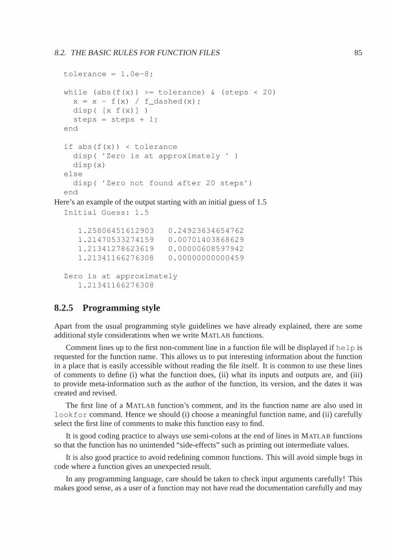
8.2. THE BASIC RULES FOR FUNCTION FILES 85
tolerance = 1.0e-8;
while (abs(f(x)) >= tolerance) & (steps < 20)x = x - f(x) / f_dashed(x);disp( [x f(x)] )steps = steps + 1;
end
if abs(f(x)) < tolerancedisp( ’Zero is at approximately ’ )disp(x)
elsedisp( ’Zero not found after 20 steps’)
endHere’s an example of the output starting with an initial guess of 1.5
Initial Guess: 1.5
1.25806451612903 0.249236346547621.21470533274159 0.007014038686291.21341278623619 0.000006085979421.21341166276308 0.00000000000459
Zero is at approximately1.21341166276308
8.2.5 Programming style
Apart from the usual programming style guidelines we have already explained, there are someadditional style considerations when we write MATLAB functions.
Comment lines up to the first non-comment line in a function file will be displayed ifhelp isrequested for the function name. This allows us to put interesting information about the functionin a place that is easily accessible without reading the file itself. It is common to use these linesof comments to define (i) what the function does, (ii) what itsinputs and outputs are, and (iii)to provide meta-information such as the author of the function, its version, and the dates it wascreated and revised.
The first line of a MATLAB function’s comment, and its the function name are also used inlookfor command. Hence we should (i) choose a meaningful function name, and (ii) carefullyselect the first line of comments to make this function easy tofind.
It is good coding practice to always use semi-colons at the end of lines in MATLAB functionsso that the function has no unintended “side-effects” such as printing out intermediate values.
It is also good practice to avoid redefining common functions. This will avoid simple bugs incode where a function gives an unexpected result.
In any programming language, care should be taken to check input arguments carefully! Thismakes good sense, as a user of a function may not have read the documentation carefully and may

86 CHAPTER 8. DEFINING FUNCTIONS WITH M-FILES
make a mistake in calling the function. Also, failing to check validity of input arguments is amajor source of security holes in various pieces of computercode. We generally omit such checksin our examples, to keep them short and simple, but they should not be omitted in practice.
Finally, we should (almost) never use global variables.
8.3 Function names as input variables withfeval
It is possible that we don’t know the function we wish to call when we are writing our program.For instance, we might wish to use Newton’s method (above) for a function that a user inputs. Weneed a way of computing the result of a function, where the function name is held in a variable.To do so we use thefeval function, for instance:
feval( ’sqrt’,9)
would give the answer 3 (the square root of 9). Sofeval(’sqrt’,x) is the same assqrt(x) !
The first argument offeval is astring(i.e. a name enclosed within single quotes) representingthe function to be evaluated. The subsequent inputs tofeval acts as inputs to the function ofinterest.
In our earlier Newton iteration scheme it would be useful if we could write a general script thataccepts the function as an input variable – this would make the script that much more general (anduseful). We would therefore like to callnewton as follows:
x0 = 1.5;[x f conv] = newton( ’f’, ’f_dashed’, x0)
where’f’ and’f dashed’ are the names of the function M-files containingf(x) andf ′(x) thatwe previously defined, andx0 is the initial guess. The outputs are the approximate location of thezero, the function value at the zero (which should be close tozero) and a variableconverged toindicate whether or not the output process has converged. The complete, new, M-filenewton.mis as follows:
function [ x, f, converged] = newton(fn, derivative_fn, x0)% Newton iteration% Performs Newton iteration to find the root of% function fn with derivative derivative_fn.% Initial guess is x0. Returns the final value of% x and f(x) and the flag converged (1 =% convergence, 0 = divergence).
steps = 0;tolerance = 1.0e-8;x = x0;
while (abs(feval(fn,x)) >= tolerance) & (steps<20)x = x - feval(fn,x) / feval(derivative_fn,x);disp( [x feval(fn,x)] )steps = steps + 1;

8.4. INLINE AND ANONYMOUS FUNCTIONS 87
end
f = feval(fn,x);if (abs(f) < tolerance)
converged = 1;else
converged = 0;end
Now we can call the function as required above, i.e.,x0 = 1.5;[x f conv] = newton( ’f’, ’f_dashed’, x0)
but we could also call it asx0 = 1.5;[x f conv] = newton( ’sin’, ’cos’, x0)
and we would now find a zero of the sine function. This gives us alot more power to createnumerical routines that are not tied to particular functions, but can instead take the function ofinterest as a input. This is a common approach for many optimization routines or DE solvers.
An alternative, slightly more general, method to implementthe same process is to usefunctionhandles. We can obtain a handle to a function using the@symbol. The handle is analogous to apointer inC, but it is outside the scope of this course, so we shall simplynote that more informationcan be found usinghelp function_handle .
8.4 Inline and anonymous functions
Sometimes, we have a very short function that we want to use several times in a program, but don’tthink is worth creating a separate.m file for. We can use aninline function for such a function.
cube=inline(’xˆ3’); % define the inline functiony = cube(3);
The above code would sety = 27, the cube of 3.
The function (and its input arguments) is specified implicitly in the string ’xˆ3’ . Inlinefunctions don’t leave much space for comments, and are not always as clear as a proper.m file, sowe generally avoid their use except for trivial functions.
Anonymous functions are functions without a name. MATLAB has methods for constructingsuch functions, and keeping a reference (a handle) to them without a name, but these are beyondthe scope of this course.
8.5 Recursion
Many mathematical functions are definedrecursively, that is, they are defined in terms of them-selves. For instance, the factorial function may be defined recursively as
n! = n × (n − 1)!

88 CHAPTER 8. DEFINING FUNCTIONS WITH M-FILES
provided we define0! = 1. MATLAB allows functions to call themselves; a process that is calledrecursion. We can write a M-file for the factorial function,fact.m :
function y = fact(n)% Factorial function% Recursive evaluation of n!
if n == 0y = 1;
elsey = n * fact(n-1);
end
The above function simply calculates the value of0! to be 1, but when we call it forn > 0,it calculates the value by calling itself again. The programterminates (for non-negative integerinputs) because each time it decrements the input argument to the recursive call of itself.
In general recursion isnotefficient. An iterative approach to the same calculation, e.g.,
function y = fact(n)% Factorial function% Iterative evaluation of n!
y = 1;for i=1:n
y = y * i;end
would be much faster. In fact, because of the additional memory used by all of those function calls,the recursive approach may fail for largen. In addition, a great deal of care must be taken that therecursion terminates, and we don’t fall into an infinite recursion. The recursive implementation offactorial given above would fall into infinite recursion if the input argument is not an integer. Careshould be taken to check input arguments carefully!
In point of fact, the above is still not the most efficient approach in MATLAB . We can create avectorised approach as follows:
function y = fact(n)% Factorial function% Vectorized evaluation of n!
if n == 0y = 1;
elsey = prod(1:n);
end
which would be faster again.
However, there are some programing tasks which are relatively easy using recursion, but quitehard using an iterative approach. The Tower’s of Hanoi problem is a classic case. The puzzle wasinvented by the French mathematician douard Lucas in 1883, and we describe it below.

8.5. RECURSION 89
Towers of Hanoi: There is a legend about an Indian temple which contains a large room withthree time-worn posts in it surrounded by 64 golden disks of different sizes. The priests ofBrahma, acting out the command of an ancient prophecy, have been moving these disks, inaccordance with the rules: they must move all of the disks from one post to another but maynever place a larger disk on a smaller.
The trick, in this puzzle, is to realize that to move all 64 disks, we need only move the top 63,then move the bottom disk to the third post and move the top 63 disks onto the third post as well.Likewise, we can move the 63 disk stack by first moving the 62 disk stack, and so on. Thereforethis problem has an obvious recursive implementation. The following function implements this,and illustrates how it works.
function disks = move_subtower(disks, n, i, j, do_plot);% move a subtower of size n from post i to j
if (nargin < 5)do_plot = 0;
end
if (do_plot)plot_disks(disks);pause;
end
if (n==1)disks = move_disks(disks, i, j);
elsek = setdiff([1:3], [i j]);disks = move_subtower(disks, n-1, i, k);if (do_plot)
plot_disks(disks);pause;
end
disks = move_disks(disks, i, j);if (do_plot)
plot_disks(disks);pause;
end
disks = move_subtower(disks, n-1, k, j);if (do_plot)
plot_disks(disks);pause;
end

90 CHAPTER 8. DEFINING FUNCTIONS WITH M-FILES
end
The inputs are a vector giving the pole each disk is on (assuming they are in order of size), thenumber of disks to move, and the two posts we wish to move a stack between, plus an optionalargument that will allow us to plot the results. The functionuses two other functions, one thatmoves individual disksmove_disks ,
function disks=move_disks(disks, i, j);% move the top disk from post i to post j% really should also check for errorsk = max(find(disks == i));disks(k) = j;
and one to plot the towersplot_disks ,
function plot_disks(disks);% plots disks
n = length(disks);
figure(1)hold offplot(0,0)hold onfor i=1:3
plot([i i], [0 n+1], ...’k’, ’linewidth’, 10);
endset(gca, ’xlim’, [0 4]);set(gca, ’ylim’, [0 n+2]);
n_disks = 0.5 * ones(3,1);for i=1:n
disk_ra = 0.5 * (1 - i/(n+1));post = disks(i);plot([post-disk_ra post+disk_ra], ...
[n_disks(post) n_disks(post)], ...’linewidth’, 20);
n_disks(post) = n_disks(post) + 1;end
We would call the function as follows:N = 7; % do a stack of 7 disksdisks = ones(N,1); % initially all disks are on post 1plot_disks(move_subtower(disks, N, 1, 3, 1));

8.5. RECURSION 91
Note, however, that this program makes two recursive calls for each level of the tower to bemoved, so the total number of recursive calls for a tower of height N would be2N , which growsquite quickly. For instance, so a stack of 64 disks, we would require264 ≃ 2× 10¹⁹ function calls.The universe is not in any immediate danger!

92 CHAPTER 8. DEFINING FUNCTIONS WITH M-FILES

Chapter 9
0-1 vectors
As we have seen, MATLAB is more efficient when we can use vector operations instead offorloops. Vectorization of matrix of some operations is very natural, but other operations need somethought. In particular, the best approach to vectorise conditional statements (if-else ’s) is notalways obvious. One handy trick is the use of logical vectors(vectors of logical variables). Logicalvariables are represented in MATLAB as 0’s (FALSE) and 1’s (TRUE), and so we sometimes callthese0-1 vectorsand matrices. To introduce this concept first carry out the following at theMATLAB prompt:
r = 0:0.2:1z = (r <= 0.5)
When vectors are involved in logical expressions such as thesecond step above, the comparisonis carried outterm-by-term. The brackets are not necessary, but make the statement morereadableby clarifying that a logical vector is being assigned toz . If the comparison is true for a particularelement of the vector, the resulting vector has a1 in the corresponding position, otherwise it has a0. Thus the response to these commands will be
r =0 0.2000 0.4000 0.6000 0.8000 1.0000
z =1 1 1 0 0 0
We can see that the vectorr is constructed to take values from 0 to 1 in steps of 0.2. The vectorlogical z takes values of 1, where1 is less than (or equal to) 0.5 and values of0 otherwise. Thewhos command returns
Name Size Bytes Class Attributes
r 1x6 48 doublez 1x6 6 logical
Note that the logical arrayz takes only 6 bytes (one byte for each term in the vector), and so it ismuch more compact than a double array (though it could be morecompact still as it onlyneeds1byte for each eight elements).
We can easily construct other 0-1 vectors, e.g.,
93

94 CHAPTER 9. 0-1 VECTORS
r = 0:0.2:1;z = r == 0.4
which returns
z =0 0 1 0 0 0
Note that in the statement the first= sign is an assignment operator (it assigns the value of theright-hand side to the variablez ). The second “double”== is thecomparisonoperator that testswherer is equal to 0.4.
We can use vector and matrix operations to work on logicals just as we can for other variables,for instance a. * product acts like and AND operation, e.g.,
r = 0:0.2:1;z = (r <= 0.5)y = (r >= 0.2)x = z . * y
results in
z =1 1 1 0 0 0
y =0 1 1 1 1 1
x =0 1 1 0 0 0
We could have obtained the same result with
x = z & y
where& is MATLAB ’s AND operator. Other logical and arithmetic operators canbe combined toconstruct more complicated expressions. Combinations of logical and numerical vectors can alsobe used to great effect as we shall see in the following examples.
9.1 Combining logical and numerical vectors
The key to vectorization of conditional statements is the combination of logical and numericalexpressions. We explore this through several examples.
9.1.1 Avoiding division by zero:
Suppose we want to plot thesinc function over the rangex ∈ [−2π, 2π]. Typically we considerthe sinc function to besin(x)/x. We can, of course, set up a vector containing thex-values
x = -2 * pi : pi / 20 : 2 * pi;
and then calculate

9.1. COMBINING LOGICAL AND NUMERICAL VECTORS 95
y = sin(x) ./ x;
In this case MATLAB will return the error messageWarning: Divide by zero and atx = 0 the vectory will contain NaN(Not a Number).
However, the precise definition of the sinc function is
sinc(x) =
{
sin(x)/x, x 6= 01 x = 1
The formal definition above explicitly removes the problem at x = 0. We can easily check thatthe resulting function is continuous, and defined everywhere, hence the limit asx → 0 of the sincfunction is 1. We exploit this by computing the function at a value very close to zero, rather thanat zero. We will replace the element wherex==0 by x = eps . This is a special MATLAB valuethat is defined at the difference between1 and the next largest number that can be represented inMATLAB ; it has the valueeps = 2.220446049250313e-16 . To remove the troublesome0from x we can use
x = x + ( x == 0) * eps;
The expressionx == 0 returns a 0-1 vector with a single1 in the position corresponding to thezero element;eps is only added to this value, so that the new vector is identical to the old, exceptthat it no longer has a zero value anywhere. We can now plot thegraph of sinc(x) correctly using
x = -2 * pi : pi / 20 : 2 * pi;x = x + ( x == 0) * eps; % change x=0 to x=epsy = sin(x) ./ x;plot(x,y)
The beauty of the above approach is we don’t assume thatx is equal to zero anywhere. If no termof the vector is ever zero, then the statementx = x + ( x == 0) * eps; has no affect. Itonly effects those places wherex==0 .
9.1.2 Using 0-1 vectors to replaceelse-if ladders
Income tax in Australia depends in a non-linear way on your income. As your income increase,the marginal tax— the tax you pay in each extra dollar of income — increases in aseries ofsteps. The rates, as of 2007-2008 are given athttp://www.ato.gov.au/individuals/content.asp?doc=/content/12333.htm&mnu=5464&mfp=001 /002 as
Taxable Income Marginal Tax Rate Total Payment<$6,000 0.00 Nil$6,001-$30,000 0.15 15c for each $1 between $6,000-$30,000$30,001-$75,000 0.30 +30c for each $1 between $30,000-$75,000$75,001-$150,000 0.40 +40c for each $1 between $75,000-$150,000>$150,001 0.45 +45c for each $1 over $150,000
ignoring the medicare levy. The above table expressed income tax rates in the standard formpresented to the public, but another way to write these is to look at the ratedifferences, e.g., the

96 CHAPTER 9. 0-1 VECTORS
difference between the tax bracket from $30,000-75,000 and$6,000-30,000 is0.3 − 0.15 = 0.15.For each dollar above the relevant tax bracket we pay this extra differencein the income tax. Intabular form:
Taxable Income Difference Total Payment<$6,000 0.00 Nil$6,001-$30,000 0.15 15c for each $1 above $6,000$30,001-$75,000 0.15 +15c for each $1 above $30,000$75,001-$150,000 0.10 +10c for each $1 above $75,000>$150,001 0.05 +5c for each $1 above $150,000
The naive approach to this calculation would be to use a complex series ofif statements in anif-else ladder. Note that we use thediff function to calculate the tax rate differences.
tax_rate = [0 0.15 0.30 0.40 0.45];tax_rate_diff = diff(tax_rate);tax_threshold = [6000 30000 75000 150000];income_tax = 0;if (income > tax_threshold(1))
income_tax = (income-tax_threshold(1)) * tax_rate_diff(1);if (income > tax_threshold(2))
income_tax = income_tax + (income-tax_threshold(2)) ...
* tax_rate_diff(2);if (income > tax_threshold(3))
income_tax = income_tax + (income-tax_threshold(3)) ...
* tax_rate_diff(3);if (income > tax_threshold(4))
income_tax = income_tax + (income-tax_threshold(4)) ...
* tax_rate_diff(4);end
endend
end
Imagine that we were the tax office and wished to calculate theincome tax for all 20 million or soAustralians. In this case the variableincome would be a vector. Given theif statements above,the only viable approach would be to put a (very) bigfor loop around the above code. As weknow, in MATLAB this will be inefficient. It is also inelegant – for instance it assumes that thenumber of tax brackets will not change. The better option in MATLAB is to use a combination oflogical and numerical operations.
We can replace this complex series of statements with a much shorter piece of code, which wegiven in the form of a function.m file below.
function tax = income_tax(taxable_income)% Calculate income tax.%% file: tax.m, (c) Matthew Roughan, Thu Apr 10 2008
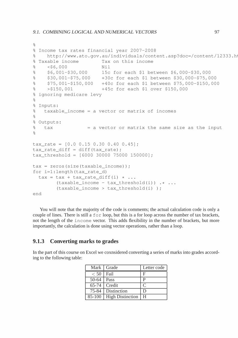
9.1. COMBINING LOGICAL AND NUMERICAL VECTORS 97
%% Income tax rates financial year 2007-2008% http://www.ato.gov.au/individuals/content.asp?doc= /content/12333.htm&% Taxable income Tax on this income% <$6,000 Nil% $6,001-$30,000 15c for each $1 between $6,000-$30,000% $30,001-$75,000 +30c for each $1 between $30,000-$75,000% $75,001-$150,000 +40c for each $1 between $75,000-$150,0 00% >$150,001 +45c for each $1 over $150,000% ignoring medicare levy%% Inputs:% taxable_income = a vector or matrix of incomes%% Outputs:% tax = a vector or matrix the same size as the input%
tax_rate = [0.0 0.15 0.30 0.40 0.45];tax_rate_diff = diff(tax_rate);tax_threshold = [6000 30000 75000 150000];
tax = zeros(size(taxable_income));for i=1:length(tax_rate_d)
tax = tax + tax_rate_diff(i) * ...(taxable_income - tax_threshold(i)) . * ...(taxable_income > tax_threshold(i) );
end
You will note that the majority of the code is comments; the actual calculation code is only acouple of lines. There is still afor loop, but this is a for loop across the number of tax brackets,not the length of theincome vector. This adds flexibility in the number of brackets, but moreimportantly, the calculation is done using vector operations, rather than a loop.
9.1.3 Converting marks to grades
In the part of this course on Excel we coxnsidered convertinga series of marks into grades accord-ing to the following table:
Mark Grade Letter code< 50 Fail F
50-64 Pass P65-74 Credit C75-84 Distinction D
85-100 High Distinction H

98 CHAPTER 9. 0-1 VECTORS
Here we denote each grade by a single letter code, and we seek to construct a vector of such codesfrom a vector of marks. The following code does so:
mark = 100 * rand(100,1); % generate 100 random marks between 0-100grade = (mark < 50) * ’F’ + ...
(mark >= 50 & mark < 65) * ’P’ + ...(mark >= 65 & mark < 75) * ’C’ + ...(mark >= 75 & mark < 85) * ’D’ + ...(mark >= 85) * ’H’;
grade = char(grade)
The code relies on the fact that we can treat characters as numbers, and that the logical vectorsbeing constructed will not overlap (i.e., the intersectionof values where more than one is true isempty). The final step converts the numbers back into characters.
9.2 Additional tests
We can test ifall of the elements of a logical vector are true using theprod command as follows:
check_all = (prod(some_logical_vector) == 1)
The logical variablecheck_all will take the value 1, iff all of the elements of the vectorsome_logical_vector are 1, and it will otherwise be 0. We can test ifat leastone of alogical vector is true using thesum function, e.g.,
check_at_least = (sum(some_logical_vector) > 0)
The variablecheck_at_least will take the value 1 if at least one of the elements of the vectorsome_logical_vector is 1, and 0 otherwise.
9.3 Thefind function
An important function, in the context of logical vectors, isthefind function. The function returnsthe indices at which a logical vector is true. For example:
r = 0:0.2:1;z = find(r <= 0.5)
will return
z =1 2 3
This indicates that the conditionr <= 0.5 is true for the first terms of the vectorr . Anothersimple example is
r = 0:0.2:1;z = find(r == 0.4)
which returns
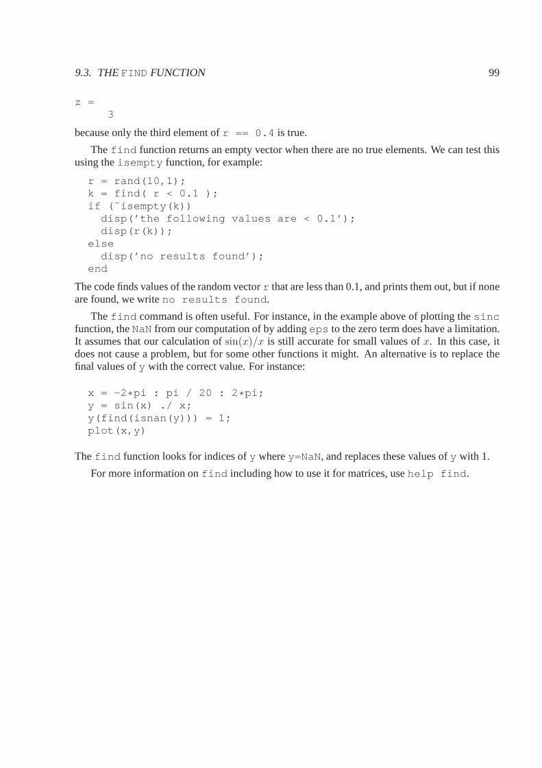
9.3. THEFIND FUNCTION 99
z =3
because only the third element ofr == 0.4 is true.
The find function returns an empty vector when there are no true elements. We can test thisusing theisempty function, for example:
r = rand(10,1);k = find( r < 0.1 );if (˜isempty(k))
disp(’the following values are < 0.1’);disp(r(k));
elsedisp(’no results found’);
end
The code finds values of the random vectorr that are less than 0.1, and prints them out, but if noneare found, we writeno results found .
The find command is often useful. For instance, in the example above of plotting thesincfunction, theNaNfrom our computation of by addingeps to the zero term does have a limitation.It assumes that our calculation ofsin(x)/x is still accurate for small values ofx. In this case, itdoes not cause a problem, but for some other functions it might. An alternative is to replace thefinal values ofy with the correct value. For instance:
x = -2 * pi : pi / 20 : 2 * pi;y = sin(x) ./ x;y(find(isnan(y))) = 1;plot(x,y)
Thefind function looks for indices ofy wherey=NaN, and replaces these values ofy with 1.
For more information onfind including how to use it for matrices, usehelp find .

100 CHAPTER 9. 0-1 VECTORS

Chapter 10
The Optimization Toolbox
Toolboxes add extra functionality to MATLAB . One extremely useful toolbox is the OptimizationToolbox. We can use this to solve a variety of optimization problems, such as those discussed ear-lier. However, we don’t need it for simple problems. As notedearlier, we can program a bisectionsearch (or other) to find zeros and other function propertiessuch as maxima. The place wherethe optimization toolbox comes into its own is where we have complex optimizations problems,for instance of the linear programming type. We will consider this case below, but note that theOptimization toolbox has a range of functions: seehelp optim for more details.
10.1 Linear Programming
We now consider a problem where we have more than one variable, a linear objective function,and a series of linear constraints. We call such a problem alinear program , and there are goodreasons to consider such problems, and good techniques for their solution.
This particular example came out of Ragsdale, page 20. The problems originates from a hy-pothetical company Blue Ridge Hot Tubs that sells two types of hot-tubs (saunas): Aqua-Spa andHydro-Lux. The manager of BRHT needs to know how many of each tub to produce.
She wishes to maximise her profit each cycle [each month, say]subject to supply constraints[on labour and inputs]. Each hot tub needs one pump and the supply of pumps is at most 200 permonth. The Aqua-Spa tub needs 12 feet of copper tubing in its construction, while the Hydro-Luxuses 16 feet and we can only get 2889 feet of tubing per month. Each Aqua-Spa tub needs 9 hoursof labour to construct, while the Hydro-Lux needs 6 hours, but there are only 1566 man hours ofworkers available per month. [BTW Aqua is water in Latin, Hydro is water in Greek (cute!)]. Theprofit from the sale of an Aqua-Spa tub is $350 and for the Hydro-Lux tub $300.
We now introduce decisionx1 andx2 which represent the number of Aqua-Spa tubs and thenumber of Hydro-Lux tubs made in each cycle. We then wish to maximise the profit
P = 350x1 + 300x2
101

102 CHAPTER 10. THE OPTIMIZATION TOOLBOX
subject to the constraints
x1 + x2 ≤ 200
12x1 + 16x2 ≤ 2889
9x1 + 6x2 ≤ 1566
and of coursex1 ≥ 0 andx2 ≥ 0. The first constraints says that the number of pumps is limited to200, the second refers to the available copper tubing, and the third to the total available man-hours.Actually we should also require thatx1 andx2 be integers (half a hot-tun isn’t worth much), butwe will won’t try to do this here.
In MATLAB , we need to represent this problem in the formminimize
f′ ∗ x
subject to the constraints
A ∗ x ≤ b
Aeq ∗ x = beq
,
andl ≤ x ≤ u. Here, we usex as a vector of the variables (in this casex1 andx2), andl andu arelower and upper bounds on the variables. In general, it is nothard to transform a linear programinto this form. Some tricks that are useful are
• If the original problem is a maximization, then we simply multiply the objective function by-1 to obtain a minimization problem.
• the vectorf used in the objective function is just given by the co-efficients in the linearobjective function, e.g., in the example
f = −(350, 300)′.
• If a constraint has a≥ sign, then we can transform it to have a≤ sign by multiplying by -1.
• If a variable doesn’t have an upper bound, e.g., in the problem above, then we can useInfin place of a number in the vectoru. Similarly with -Inf for lower bounds.
• One or the other of the equality, or inequality constraints may be empty. In the exampleproblem there are no equalities so we setAeq = [], beq = []; .
• The rows ofA are made up of the co-efficient of the same row of the constraints, e.g., in ourexample
A =
1 112 169 6

10.2. WHY USEMATLAB FOR OPTIMIZATION 103
• the vectorb is made up of the right-hand side of the constraints, in the same order theyappear, e.g., in our example
b =
20028891566
One the problem has been constructed, we can find the optimal solution using thelinprogfunction, which is part of the Optimization Toolbox. It takes a variable number of arguments, butto solve the above problem, we would call it usingx=linprog(f,A,b,Aeq,beq,l,u) .
So in the example problem, our MATLAB code to construct and solve the linear programmingproblem would be
f = -[350; 300];A = [[ 1 1];
[12 16];[ 9 6]];
b = [200; 2889; 1566];Aeq = [];beq = [];l = zeros(2,1);u = [Inf; Inf];x = linprog(f,A,b,Aeq,beq,l,u)
which outputsOptimization terminated.x =
122.000078.0000
There are a variety of additional input terms, or output terms that one can use to specify initialsolutions, numbers of iterations, objective function values, and so on. Seehelp linprog formore details.
There are other optimization routines, both in the Optimization toolbox (e.g.fgoalattain )and elsewhere that allow us to mimic most of the possibilities in Excel, and some others as well.
10.2 Why useMATLAB for optimization
MATLAB and Excel both allow us to solve optimization problems. Whenshould we use one, orthe other. Often it is a matter of person preference – use whichever you are most comfortablewith. For many people this will be Excel, because they consider it easier to enter the optimizationproblem constraints through a spreadsheet. However, MATLAB does have distinct advantages overExcel.
• MATLAB can solve much larger optimization problems than Excel (problems with morevariables and more constraints). The exact numbers will depend on versions, and hardware,but typically we might be able to solve problems 10 times larger in MATLAB with roughlyequivalent systems. MATLAB is typically a lot faster as well.

104 CHAPTER 10. THE OPTIMIZATION TOOLBOX
• MATLAB enables the solution of many optimization problems. For instance, it is easy, inMATLAB , to write an optimization inside afor loop, and thus execute it (with some dif-ferences presumably) each time the loop is executed. For instance, each iteration mightload a new set of data from a different file. The outputs of eachoptimization could then beautomatically sent to a file.
• MATLAB facilitates using the outputs of previous programming as the inputs to our opti-mization. For instance, the constraint matrixA might be constructed using other functions.The same can be done in Excel, but if things like the number of constraints change then thisis not so easy to cope with whereas in MATLAB it is trivial.
The features make MATLAB more suitable when optimization is to be done on large problems, orfrequently, or as part of an automated system.
Finally, there are even better tools for solving optimization problems. Some can handle muchlarger problems even than MATLAB . However, one thing most other sophisticated tools have incommon is that problems are specified (mathematically) in a similar way to that above, so it isn’tgoing to waste your time to learn MATLAB ’s approach.

Chapter 11
MATLAB Roundup
11.1 More stuff
In addition to the many features which we have mentioned but not described in detail, MATLAB hasmany other features we have not discussed at all:
• MATLAB has a large array of mathematical functions not mentioned here for many tasks.Toolboxes add to this functionality considerably.
• Ability to build new GUIs for specific tasks;
• MATLAB has built in debugging, lint and profiling tools.
• Lots of technicalities,e.g.,function overloading:it is possible to have two functions withthe same name, where the one that is called depends on the input arguments;persistentvariables:variables with local scope that can keep a value in between function calls; errorhandling; and so on.
• An interface toC, so that C-code can be used directly from MATLAB (see MEX files). Also,MATLAB has interfaces to the system in which it runs (i.e., it can call other programs).
• There are alternative data structures such asstruct which allows a more object orientedapproach in MATLAB , and acell array which allows us to construct arrays of any otherdatatype, e.g. strings.
• There are many toolboxes which come complete with additional function and features in-cluding, for instance, the parallel processing toolbox, and symbolic manipulation toolbox.
11.2 Limitations
MATLAB does have limitations:
105

106 CHAPTER 11. MATLAB ROUNDUP
• It is much faster than Excel, but still not the fastest possible way to program. Where multiplynested loops are needed, there are faster ways of programming. If vector/matrix operationsare used, it can be quite fast, but still better performance may be achieved through carefullyoptimized low-level code.
• MATLAB is not particularly efficient in its (default) storage of variables. The standard is toalways used double precision floating point, which is good much of the time, but may beoverkill at 64 bits per variable.
• MATLAB ’s string handling is not the easiest to program – there are better tools such as Perl.
• Lack of associative arrays (hashes) is sometimes annoying (to me).
• MATLAB will have trouble if you need to access low-level machine dependent components,such as registers.
11.3 Summary
MATLAB also shows us the same set of concepts that we first saw in Excel, i.e.:
• variables: a value that we can change or control. In MATLAB , variables can have almostarbitrary names that we choose. MATLAB variables are different from Excel variables inthat they have atype , which we can access (viawhos) or change, to effect the amount ofmemory stored, or the accuracy of floating point numbers. However, MATLAB cannot storea formula into a variable (though a reference to a function can be).
• vectors, and matrices:are a standard data structure in most computing environments, andof great use in maths, in particular when we have a group of numbers. MATLAB allows usto store vectors and matrices into variables.
• functions:are a useful way of representing something (usually mathematical) that we wantto do with some data.
• reference:is how we include other data into our functions. In MATLAB , we make a referenceto a variable explicitly when calling a function, or using a variable’s value in an expression.
• graphing:can be used to visualise data in various ways.
• mapping: values from say a number to a grade can be easily performed using conditionalstatements (e.g.if ).
• sorting: data into order, either numerically, or alphabetically.
• filtering: to see only values that match a particular criteria. In MATLAB we do this using0-1 vectors.
• optimisation: where we seek to maximise or minimise some quantity (e.g. profit, or rev-enue).

11.3. SUMMARY 107
• constraints:limits on our variables.
• iteration:, i.e., repeating some set of steps. MATLAB provides explicit constructs for itera-tion (e.g.for andwhile loops).
• conditionals:in MATLAB are expressed via anif statement allow us to execute code con-ditional on variables.
In MATLAB these concepts are often more explicit in that they are supported by specific languageconstructs, rather than implicitly, or by function calls asthey are in Excel.
There are additional concepts we have seen here, such as
• vectorization: writing formula such that they can be applied to vectors canspeed up calcu-lation not just in MATLAB , but also in specific graphics applications, and other areas.
• modularity: breaking code into meaningful modules (in MATLAB we use functions to dothis).
• scope: variables defined inside a MATLAB function cannot be seen outside of this functionunless they are explicitly given global scope. This avoids name collisions.
• recursion: a function may call itself, and we call this type of functiona recursive function.
• performance: most tasks can be implemented in many different ways. Part of the job of aprogrammer is implementing the program efficiently.
• style: correctness is not the only task when writing code. We also need to write read-able/maintainable code, and coding style can help this dramatically.


![HOME [jhigginsholdings.com]jhigginsholdings.com/assets/coastalcomfort.pdf · 2013. 4. 24. · Christina Roughan, Karen Williams Contributing Photographers Michael Biondo, Orion Bishop,](https://static.fdocuments.net/doc/165x107/606f853b7da6a5039e1bfce7/home-2013-4-24-christina-roughan-karen-williams-contributing-photographers.jpg)