Introduction to Latent Class Regression - The Medical...
52
Latent Class Regression Statistics for Psychosocial Research II: Structural Models December 4 and 6, 2006
Transcript of Introduction to Latent Class Regression - The Medical...

Latent Class Regression
Statistics for Psychosocial Research II: Structural Models
December 4 and 6, 2006
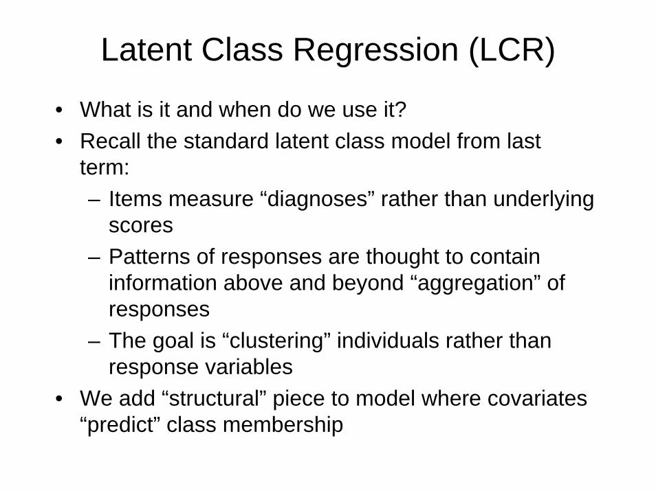
Latent Class Regression (LCR)
• What is it and when do we use it?• Recall the standard latent class model from last
term:– Items measure “diagnoses” rather than underlying
scores– Patterns of responses are thought to contain
information above and beyond “aggregation” of responses
– The goal is “clustering” individuals rather than response variables
• We add “structural” piece to model where covariates “predict” class membership

Structural Equation-type Depiction
x1
x2
x3
y3
y2
y1
y4
y5
η
Structural Piece
Measurement Piece

When to use LCR• Multiple discrete outcome variables
– binary examples• yes/no questions• present/absent symptoms
– all measuring same latent construct– We want to construct as outcome variable– Responses to questions/items measure underlying
states (i.e. classes) with error• NOT appropriate for…
– counts or other way of grouping response patterns– responses measure underlying score with error
• Note: Latent Variable is DISCRETE
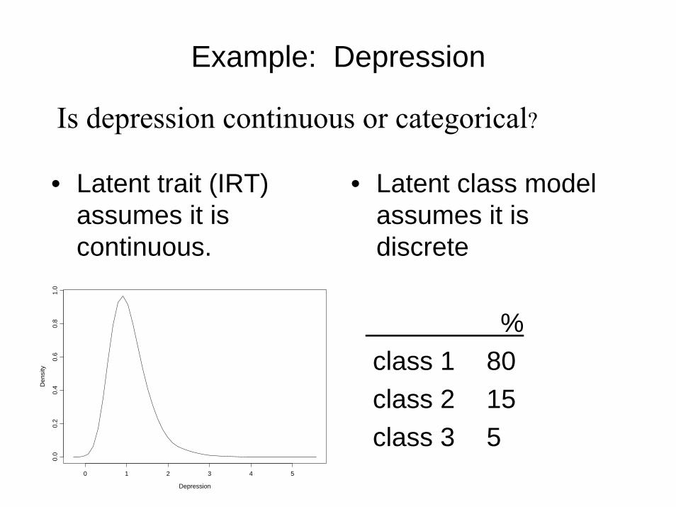
Example: Depression
• Latent trait (IRT) assumes it is continuous.
Depression
Den
sity
0 1 2 3 4 5
0.0
0.2
0.4
0.6
0.8
1.0
• Latent class model assumes it is discrete
% class 1 80class 2 15class 3 5
Is depression continuous or categorical?
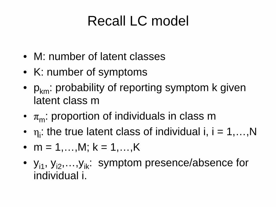
Recall LC model
• M: number of latent classes• K: number of symptoms• pkm: probability of reporting symptom k given
latent class m• πm: proportion of individuals in class m• ηi: the true latent class of individual i, i = 1,…,N• m = 1,…,M; k = 1,…,K• yi1, yi2,…,yik: symptom presence/absence for
individual i.
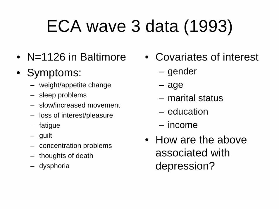
ECA wave 3 data (1993)
• N=1126 in Baltimore• Symptoms:
– weight/appetite change– sleep problems– slow/increased movement– loss of interest/pleasure– fatigue– guilt– concentration problems– thoughts of death– dysphoria
• Covariates of interest– gender– age– marital status– education– income
• How are the above associated with depression?
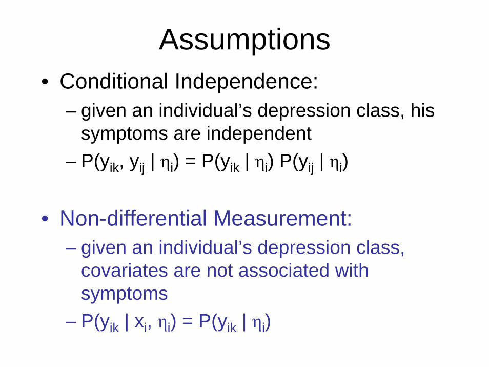
Assumptions• Conditional Independence:
– given an individual’s depression class, his symptoms are independent
– P(yik, yij | ηi) = P(yik | ηi) P(yij | ηi)
• Non-differential Measurement:– given an individual’s depression class,
covariates are not associated with symptoms
– P(yik | xi, ηi) = P(yik | ηi)
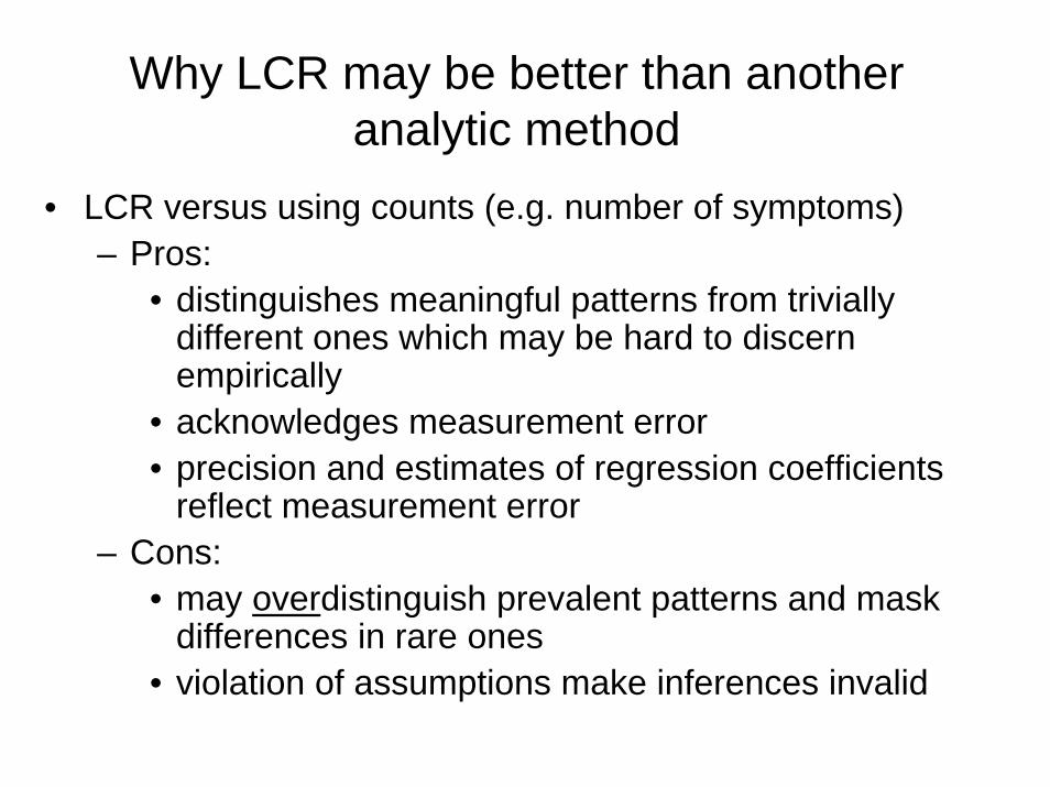
Why LCR may be better than another analytic method
• LCR versus using counts (e.g. number of symptoms)– Pros:
• distinguishes meaningful patterns from trivially different ones which may be hard to discern empirically
• acknowledges measurement error• precision and estimates of regression coefficients
reflect measurement error– Cons:
• may overdistinguish prevalent patterns and mask differences in rare ones
• violation of assumptions make inferences invalid

Why LCR may be better than another analytic method (continued)
• Versus factor-type methods– Pros:
• less severe assumptions (statistically)• easier to check assumptions
– Cons:• lose statistical power if construct is actually
dimensional (i.e. continuous)• identifiability harder to achieve (need big sample)
• Practically– Pro:
• Allows for disease/disorder classification which is useful in a treatment vs. no treatment setting

Structural Equation-type Depiction
x1
x2
x3
y3
y2
y1
y4
y5
η
Structural Piece
Measurement Piece
β p What arethe parametersthat the arrows represent?In other words,what are β andp in the LCR model?
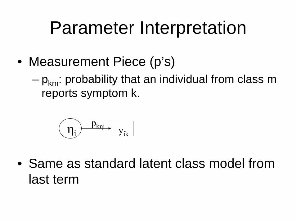
Parameter Interpretation
• Measurement Piece (p’s)– pkm: probability that an individual from class m
reports symptom k.
• Same as standard latent class model from last term
ηi yikpkηi

Parameter Interpretation
• How do we relate η’s and β’s?
• In “classic” SEM, we have linear model.
• What about when η is categorical?
• What if η is binary?
x1
x2
x3
η
β
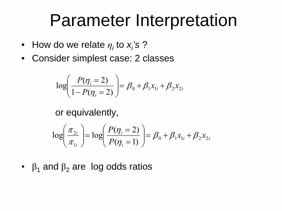
Parameter Interpretation• How do we relate ηi to xi’s ?• Consider simplest case: 2 classes
or equivalently,
• β1 and β2 are log odds ratios
iii
i xxP
P22110)2(1
)2(log βββη
η++=⎟⎟
⎠
⎞⎜⎜⎝
⎛=−
=
iii
i
i
i xxPP
221101
2
)1()2(loglog βββ
ηη
ππ
++=⎟⎟⎠
⎞⎜⎜⎝
⎛==
=⎟⎟⎠
⎞⎜⎜⎝
⎛

Model Results• p
– same as last term– KxM p’s
• πji = P(ηi = j)– Conditional on x’s– No longer ‘proportion of individuals in class’– Now, only can interpret to mean ‘probability of class
membership given covariates for individual i”– To get size of class j, can sum of πij for all i
• β– (M-1)*(H+1) β’s where H = number of covariates– M-1: one class is reference class so all of its β coefficients
are technically zero– H+1: for each class, there is one β for each covariate plus
another for the intercept.
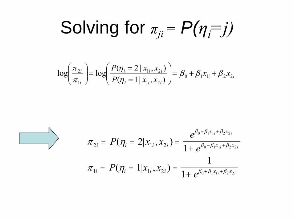
Solving for πji = P(ηi=j)
iiiii
iii
i
i xxxxPxxP
2211021
21
1
2
),|1(),|2(loglog βββ
ηη
ππ
++=⎟⎟⎠
⎞⎜⎜⎝
⎛==
=⎟⎟⎠
⎞⎜⎜⎝
⎛
π η
π η
β β β
β β β
β β β
2 1 2
1 1 2
21
11
1
0 1 1 2 2
0 1 1 2 2
0 1 1 2 2
i i i i
x x
x x
i i i i x x
P x xe
e
P x xe
i i
i i
i i
= = =+
= = =+
+ +
+ +
+ +
( | , )
( | , )

Parameter Interpretation
Example: eβ1 = 2 and x1i =1 if female, 0 if male
“Women have twice the odds of being in class 2 versus class 1 than men, holding all else constant”
eP x x cP x x c
P x x cP x x c
i i i
i i i
i i i
i i i
β ηη
ηη
12 11 1
2 01 1
1 2
1 2
1 2
1 2=
= = == = =
= = == = =
( | , )( | , )
( | , )( | , )

More than two classes?Need more than one equation Need to choose a reference class
iiiii
iii xxxxPxxP
2221120221
21
),|1(),|2(log βββ
ηη
++=⎟⎟⎠
⎞⎜⎜⎝
⎛==
iiiii
iii xxxxPxxP
2231130321
21
),|1(),|3(log βββ
ηη
++=⎟⎟⎠
⎞⎜⎜⎝
⎛==
eee e e
β
β
β β β β
12
13
13 12 13 12
=
=
= −
OR for class 2 versus class 1 for females versus males OR for class 3 versus class 1 for females versus males
= OR for class 3 versus class 2 for females versus males
/

Solving for πji = P(ηi)
iii
i
i
i xxPP
222112021
2
)1()2(loglog βββ
ηη
ππ
++=⎟⎟⎠
⎞⎜⎜⎝
⎛==
=⎟⎟⎠
⎞⎜⎜⎝
⎛
π ηβ β β
β β β β β β
β β β
β β β
2
1
3
21
02 12 1 22 2
02 12 1 22 2 03 13 1 23 2
02 12 1 22 2
0 1 1 2 2
i i
x x
x x x x
x x
x x
r
Pe
e ee
e
i i
i i i i
i i
r r i r i
= = =+ +
=
+ +
+ + + +
+ +
+ +
=∑
( )
Where we assume that 0211101 === βββ
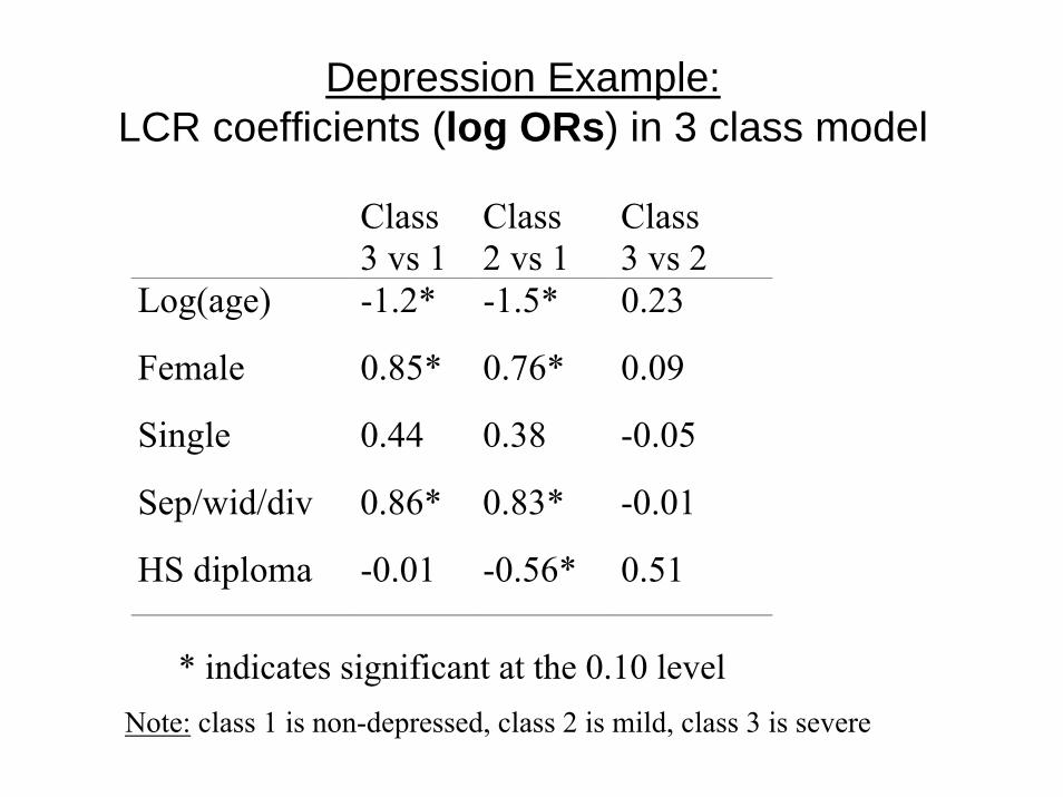
Depression Example:LCR coefficients (log ORs) in 3 class model
Class3 vs 1
Class2 vs 1
Class3 vs 2
Log(age) -1.2* -1.5* 0.23
Female 0.85* 0.76* 0.09
Single 0.44 0.38 -0.05
Sep/wid/div 0.86* 0.83* -0.01
HS diploma -0.01 -0.56* 0.51
* indicates significant at the 0.10 levelNote: class 1 is non-depressed, class 2 is mild, class 3 is severe

Depression Example:ODDS RATIOS in 3 class model
Class 3 vs 1
Class 2 vs 1
Class 3 vs 2
Log(age) 0.3* 0.22* 1.26
Female 2.34* 2.13* 1.09
Single 1.55 1.46 0.95
Sep/wid/div 2.36* 2.29* 0.99
HS diploma 0.99 0.57* 1.67
* indicates significant at the 0.10 levelNote: class 1 is non-depressed, class 2 is mild, class 3 is severe

Model Building• Step 1:
– Get the measurement part right!– Fit standard latent class model first. – Use methods we discussed last term to choose
appropriate model• Step 2:
– add covariates one at a time– It is useful to perform “simple” regressions to see
how each covariate is associated with latent variable before adjusting for others.
– Many of same issues in linear and logistic regression (e.g. multicollinearity)

Estimation• Same caveats as last term • Maximum likelihood:
– Iterative fitting procedure.– Packages
• Mplus• Splus, R• SAS
• Bayesian approach– Computationally intensive
• WinBugs• Splus, R• SAS

Properties of Estimates (β, p)
• If N is large, coefficients are approximately normal confidence intervals and Z-tests are appropriate.
• Nested models can be compared by using chi-square test.
• But, recall problems of chi-square test when sample size is large!
• And problems when the sample size is small!• Also can use AIC, BIC, etc. to compare nested
AND non-nested models (e.g. is age as continuous better than 3 age categories).

Specifics Statistically • Standard LCM Likelihood
• Latent Class Regression Likelihood
)1(
1 1
55,44,33,22,11
)1(
)()(
ikik ykm
M
m
K
k
ykmmi
iyiYiyiYiyiYiyiYiyiYiyiY
pp
PP
−
= =
======
−=
=
∑ ∏π
)1(
1 1
|55,44,33,22,11
)1()(
)()(
ikik ykm
M
m
K
k
ykmmi
xiyiYiyiYiyiYiyiYiyiYiyiY
ppx
PP
−
= =
======
−=
=
∑ ∏π
∑=
= M
m
x
x
imiim
im
e
ex
1
)(β
β
πwhere

Example: 3 class modelcoefficient estimate se 95% confidence interval
b02 -3.11 0.21 -3.52 -2.71b01 -1.80 0.15 -2.08 -1.52b2age -1.21 0.74 -2.65 0.27b3age -1.44 0.53 -2.48 -0.38b2sex 0.86 0.38 0.15 1.64b3sex 0.77 0.25 0.32 1.34
p[1,1] 0.83 0.06 0.69 0.93p[1,2] 0.40 0.05 0.31 0.50p[1,3] 0.02 0.01 0.01 0.03p[2,1] 0.84 0.061 0.72 0.94p[2,2] 0.41 0.05 0.31 0.52p[2,3] 0.02 0.01 0.01 0.04
………………etc..

Some Additional Concepts
(1) η is a NOMINAL variable
(2) Data Setup: Centering covariates can help. – Due to need to “initialize” algorithm in ML.– Due to priors on β’s in Bayesian setting– Will be meaningful in model checking, too.– Need to choose starting values for model
estimation for regression coefficients in some ML packages. This is easier if they are centered.
– Not an issue for Mplus: only need starting values for measurement part.
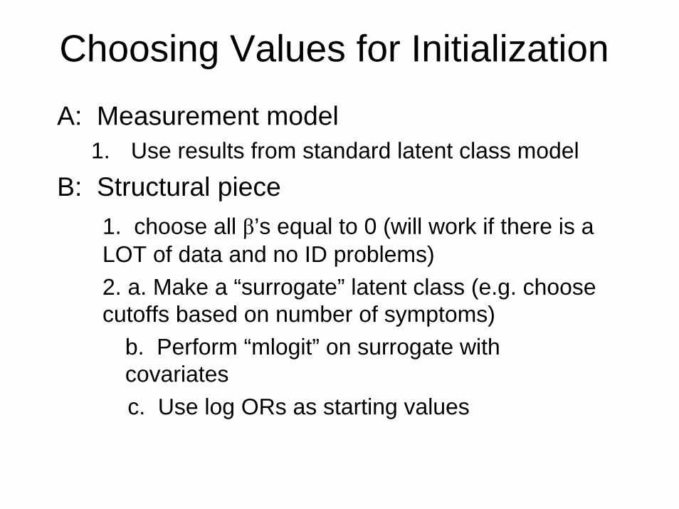
Choosing Values for Initialization
A: Measurement model1. Use results from standard latent class model
B: Structural piece1. choose all β’s equal to 0 (will work if there is a LOT of data and no ID problems)2. a. Make a “surrogate” latent class (e.g. choose cutoffs based on number of symptoms)
b. Perform “mlogit” on surrogate with covariatesc. Use log ORs as starting values
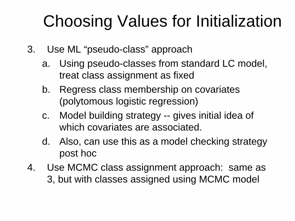
Choosing Values for Initialization3. Use ML “pseudo-class” approach
a. Using pseudo-classes from standard LC model, treat class assignment as fixed
b. Regress class membership on covariates (polytomous logistic regression)
c. Model building strategy -- gives initial idea of which covariates are associated.
d. Also, can use this as a model checking strategy post hoc
4. Use MCMC class assignment approach: same as 3, but with classes assigned using MCMC model
Important Identifiability Issue
Must run model more than once using different starting values to check identifiability!

Model Checking
• Very important step in LCR• LCR can give misleading findings if
measurement model assumptions are violated
• Two types of model checks:(1) model fit
“do y patterns behave as model would predict?”
(2) violation of assumptions“do y’s relate to x’s as expected?”

ECA wave 3 data (1993)
• N=1126 in Baltimore• Symptoms:
– weight/appetite change– sleep problems– slow/increased movement– loss of interest/pleasure– fatigue– guilt– concentration problems– thoughts of death– dysphoria
• Covariates of interest– gender– age– marital status– education– income
• How are the above associated with depression?

Models
• Model A: log(age), gender, race
• Model B: log(age), gender, race, diploma

Do y patterns behave as model predicts?
• Compare observed pattern frequencies to expected pattern frequencies
• PFC plot• How does addition of regression change
interpretation?• Evaluating fit of measurement piece
– Will be “same” as in standard LC model unless…..
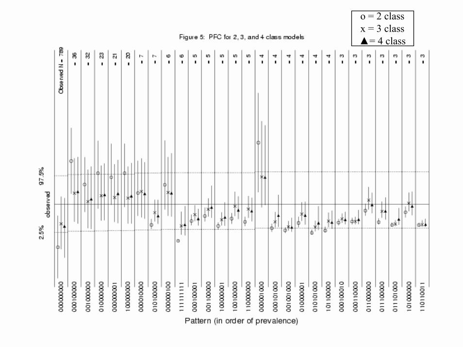
o = 2 classx = 3 class▲= 4 class

● = LCAx = LCR-Ao = LCR-B

Does pattern frequency behave as predicted by covariates?
• Idea: focus on one item at a time• Recall:
• If interested in item r, ignore (“marginalize over”) other items:
∑ ∏= =
−−===M
m
K
k
ykm
ykmiiikiKiii
kiki ppxxyYyYP1 1
)1(11 )1()()|,...,( π
∑=
−−==M
m
yrm
yrmiiiriri
kiki ppxxyYP1
)1()1()()|( π

Comparing Fitted to Observed

Categorical Covariates
• Easier than continuous (computationally)• Example
– Calculate: • Predicted males with guilt• Observed males with guilt• Predicted females with guilt• Observed females with guilt

P guilt male class P guilt class male P maleP guilt male class P class male P maleP guilt class P class male P male
pe
eP malekm
( ) ( | ) ( )( | ) ( | ) ( )( | ) ( | ) ( )
( )
and and and and
= = == = == = =
= ×+
×
2 22 2
2 2
1
0
0
β
β
• Assume LC regression model with only gender• Gender = 0 if male, 1 if female• Item of interest if guilt.• Want find how many class 2 men we would
expect to report guilt based on the model
Expected guilt male class= N pe
eP malekm( ) ( ) and and 2
1
0
0= × ×
+×
β
β
Calculate this for each of the classes and sum up: Will tell us the expected number of males reporting guilt.

Failure in Fit
• Check Assumptions– non-differential measurement– conditional independence
• Non-differential Measurement:– P(yik | xi, ηi) = P(yik | ηi) – In words, within a class, there is no
association between y’s and x’s.– Check this using logistic regression approach

Checking Non-differentialMeasurement Assumption
• For binary covariates and for each class m and item k consider
• If assumption holds, this OR will be approximately equal to 1.
• Why may this get tricky?– We don’t KNOW class assignments.– Need a strategy for assigning individuals to classes.
),0|0(/),0|1(),1|0(/),1|1(
mxyPmxyPmxyPmxyPOR
kk
kkkmx ======
=======
ηηηη
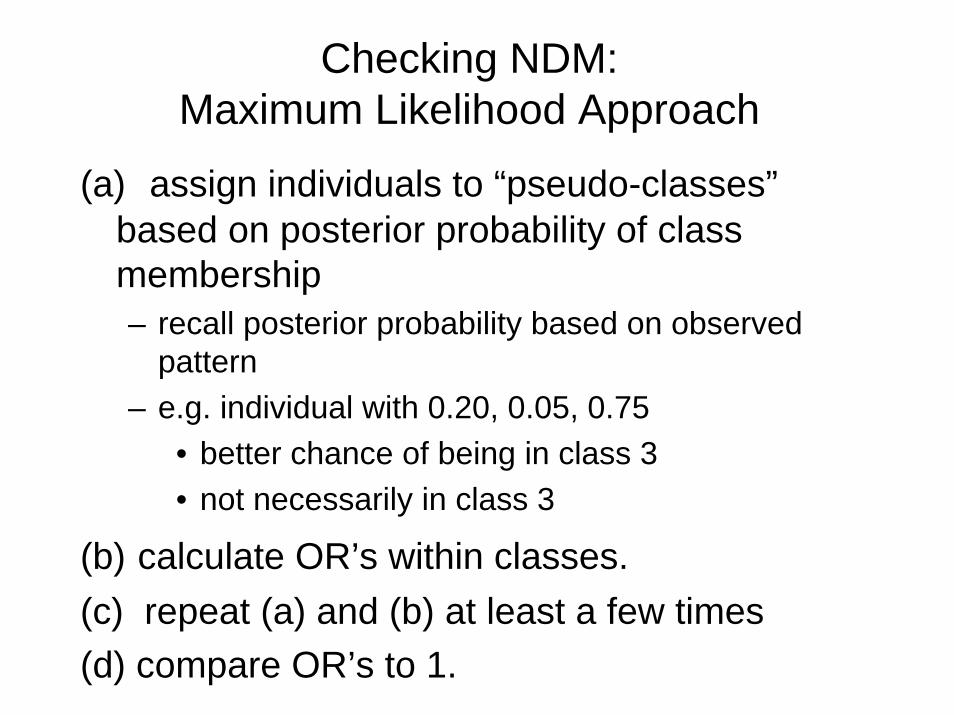
Checking NDM: Maximum Likelihood Approach
(a) assign individuals to “pseudo-classes”based on posterior probability of class membership– recall posterior probability based on observed
pattern– e.g. individual with 0.20, 0.05, 0.75
• better chance of being in class 3• not necessarily in class 3
(b) calculate OR’s within classes.(c) repeat (a) and (b) at least a few times(d) compare OR’s to 1.
Checking NDM: Maximum Likelihood Approach
• What about continuous covariates?• Use same general idea, but estimate the
logOR within classes by logistic regression• Example: age

Checking NDM: MCMC (Bayesian) approach
• At each iteration in Gibbs sampler, individuals are automatically assigned to classes no need to “manually”assign.
• At each iteration, simply calculate the OR’s of interest.
• Then, “marginalize” or average over all iterations.
• Results is posterior distribution of OR


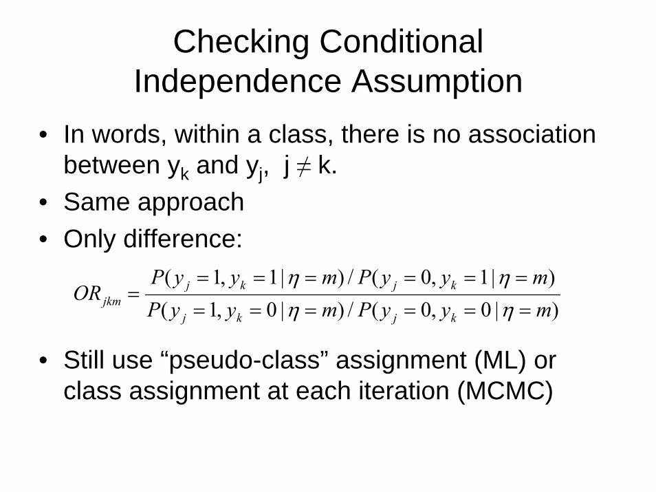
Checking ConditionalIndependence Assumption
• In words, within a class, there is no association between yk and yj, j ≠ k.
• Same approach• Only difference:
• Still use “pseudo-class” assignment (ML) or class assignment at each iteration (MCMC)
)|0,0(/)|0,1()|1,0(/)|1,1(
myyPmyyPmyyPmyyP
ORkjkj
kjkjjkm ======
=======
ηηηη


Identifiability (briefly)• General Idea: different parameters can
lead to the same model fit• 2 step rule: If
(a) polytomous logistic regression is ID’ed(b) standard LCM is ID’edThen model is ID’ed
• t-rule: need more data cells than parameters– complication: continuous covariates, but
they usually don’t make unID’ed.

Utility of Model Checking
• May modify interpretation to incorporate lack of fit/violation of assumption
• May help elucidate a transformation that that would be more appropriate (e.g. log(age) versus age)
• May lead to believe that LCR is not appropriate.