Introduction to Laplace Transforms
32
Introduction to Introduction to Laplace Transforms Laplace Transforms
-
Upload
tad-butler -
Category
Documents
-
view
144 -
download
16
description
Introduction to Laplace Transforms. Def inition of the Laplace Transform. One-sided Laplace transform :. l Some functions may not have Laplace transforms but we do not use them in circuit analysis. Choose 0 - as the lower limit (to capture discontinuity in f(t) due to an event such as - PowerPoint PPT Presentation
Transcript of Introduction to Laplace Transforms
Introduction to Introduction to Laplace TransformsLaplace Transforms
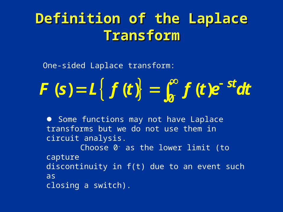
DefDefinition of the Laplace inition of the Laplace TransformTransform
Some functions may not have Laplacetransforms but we do not use them in circuit analysis. Choose 0- as the lower limit (to capturediscontinuity in f(t) due to an event such asclosing a switch).
0
( ) ( ) ( ) stF s L f t f t e dt
One-sided Laplace transform:
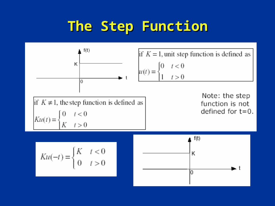
The Step FunctionThe Step Function

??
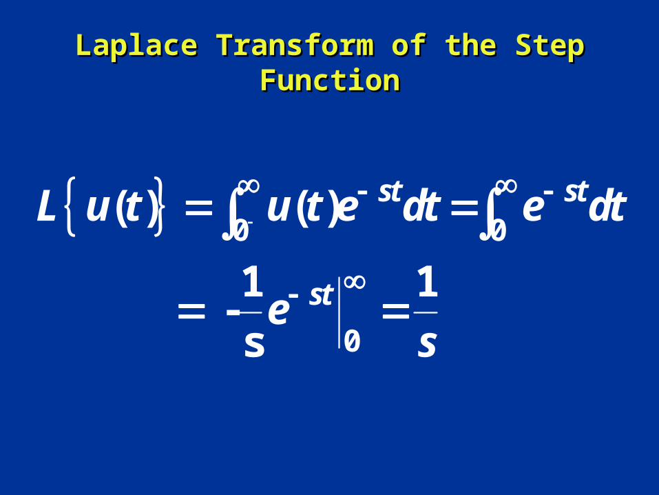
Laplace Transform of the Step Laplace Transform of the Step FunctionFunction
0 0
0
( ) ( )
1 1 -
s
st st
st
L u t u t e dt e dt
es
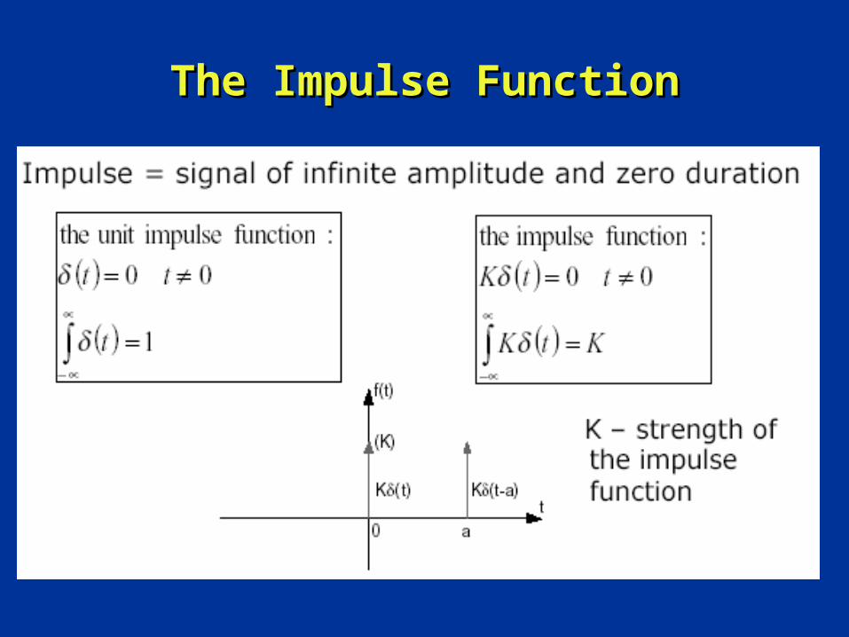
The Impulse FunctionThe Impulse Function
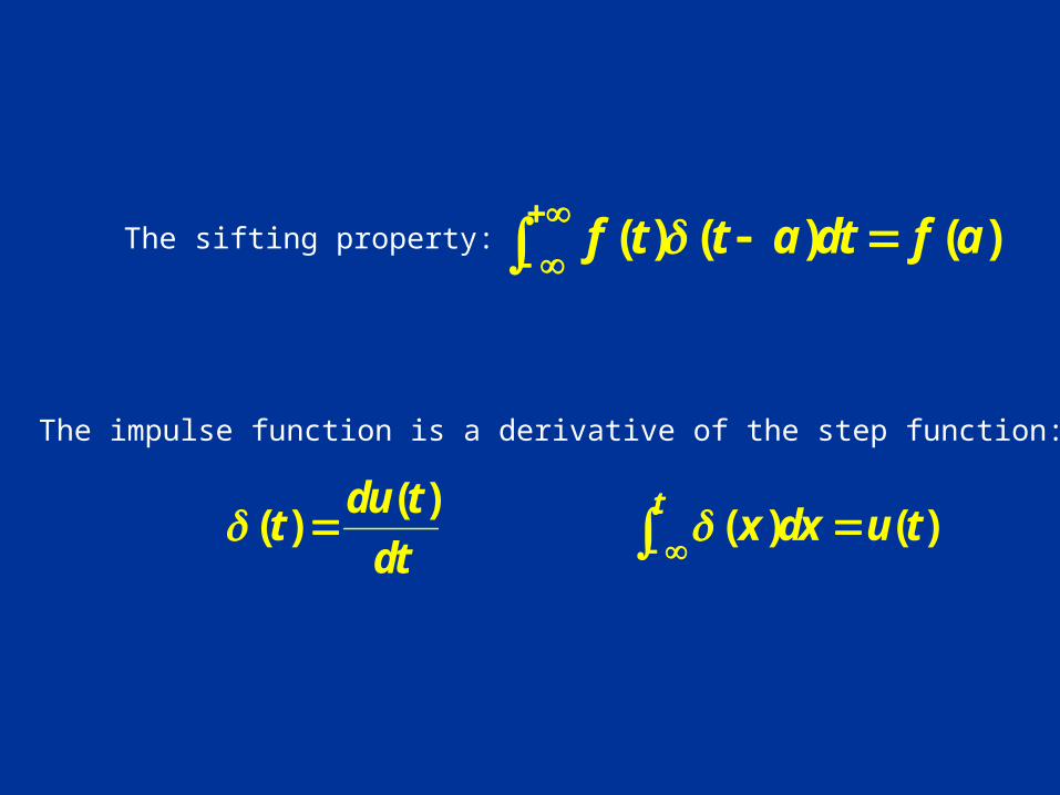
The sifting property:
The impulse function is a derivative of the step function:
( ) ( ) ( )f t t a dt f a
( )( ) ( ) ( )
tdu tt x dx u t
dt

??
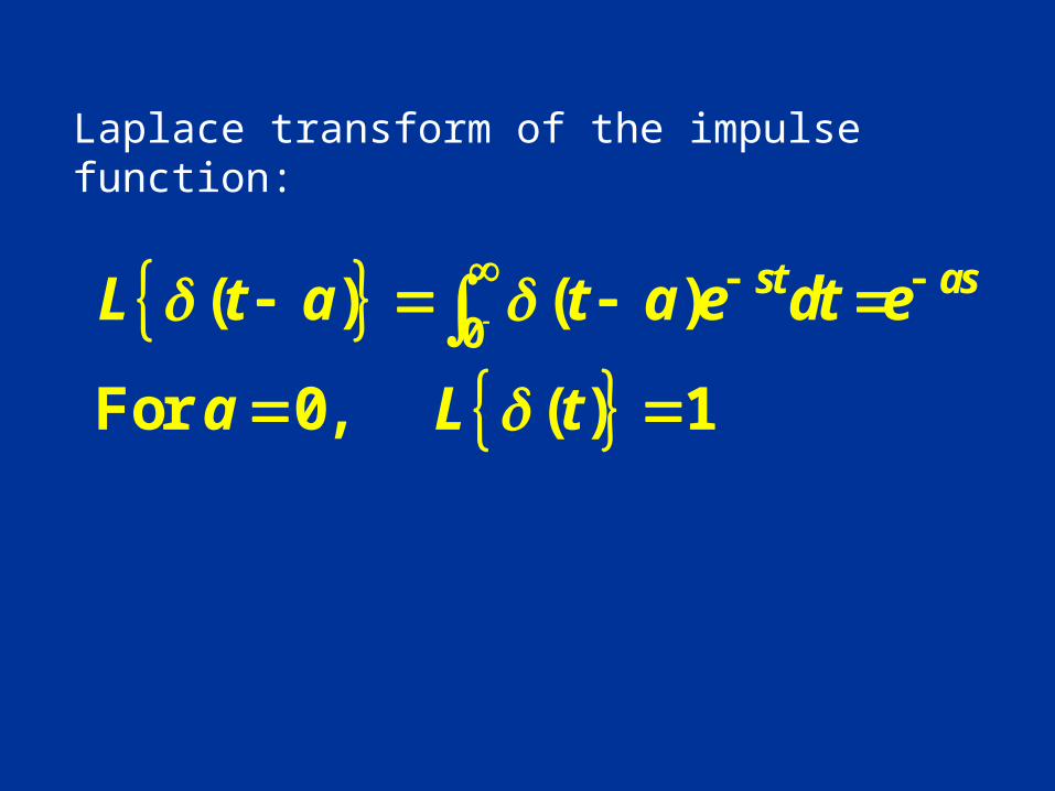
Laplace transform of the impulse function:
0( ) ( )
For 0, ( ) 1
st asL t a t a e dt e
a L t
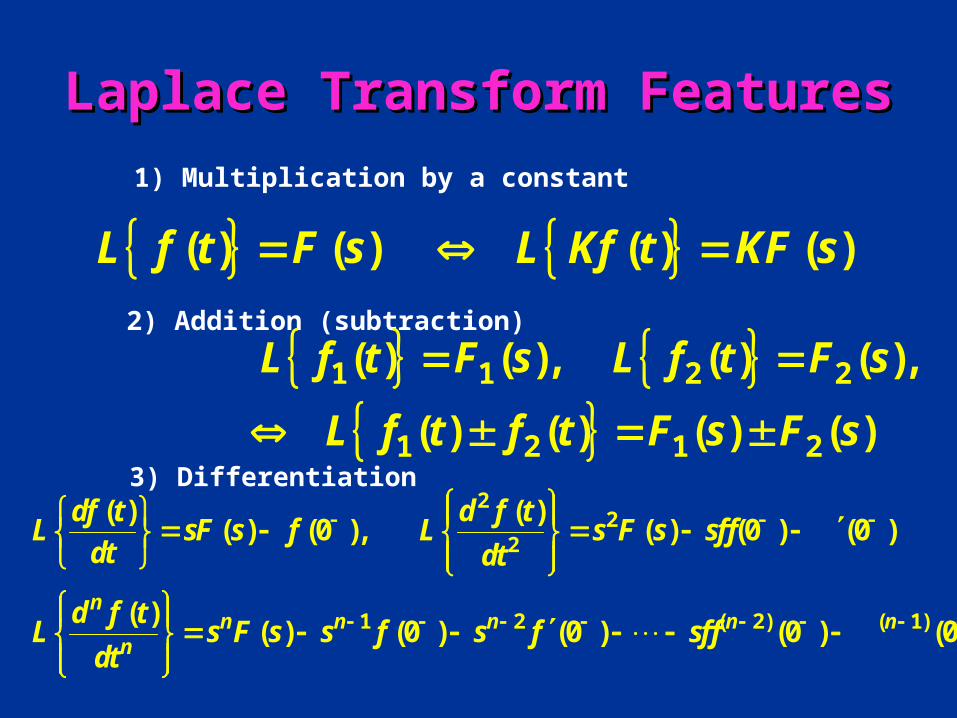
Laplace Laplace TransformTransform Features Features1) Multiplication by a constant
( ) ( ) ( ) ( ) L f t F s L Kf t KF s 2) Addition (subtraction)
1 1 2 2
1 2 1 2
( ) ( ), ( ) ( ),
( ) ( ) ( ) ( )
L f t F s L f t F s
L f t f t F s F s
3) Differentiation
22
2
1 2 ( 2) ( 1)
( ) ( )( ) (0 ), ( ) (0 ) (0 )
( )( ) (0 ) (0 ) (0 ) (0 )
nn n n n n
n
df t d f tL sF s f L s F s sf f
dt dt
d f tL s F s s f s f sf f
dt
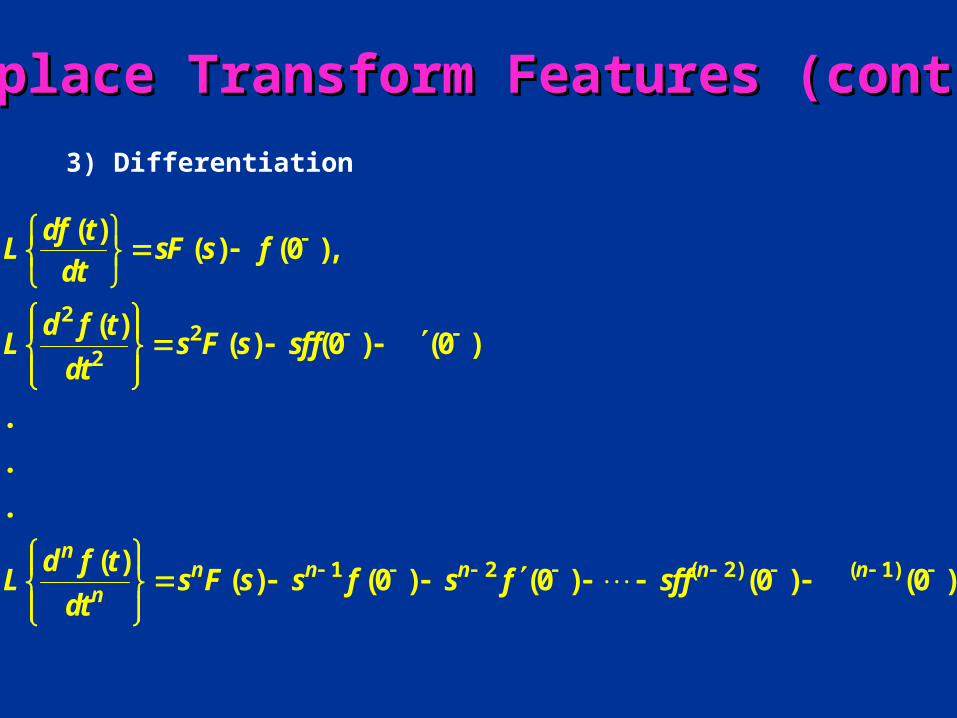
3) Differentiation
22
2
1 2 ( 2) ( 1)
( )( ) (0 ),
( )( ) (0 ) (0 )
.
.
.
( )( ) (0 ) (0 ) (0 ) (0 )
nn n n n n
n
df tL sF s f
dt
d f tL s F s sf f
dt
d f tL s F s s f s f sf f
dt
Laplace Laplace TransformTransform Features (cont.) Features (cont.)
Laplace Laplace TransformTransform Features Features (cont.)(cont.)
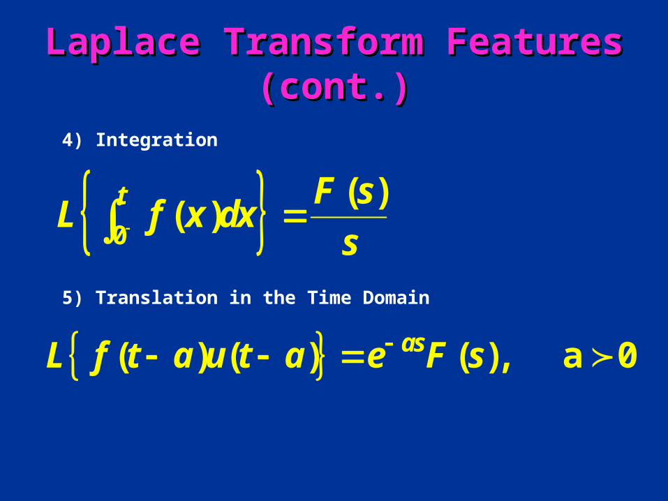
4) Integration
0
( )( )
t F sL f x dx
s
5) Translation in the Time Domain
( ) ( ) ( ), a 0asL f t a u t a e F s
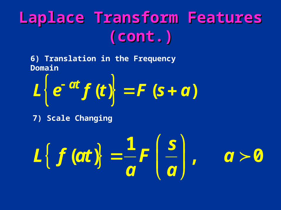
Laplace Laplace TransformTransform Features Features (cont.)(cont.)
6) Translation in the Frequency Domain
( ) ( )atL e f t F s a 7) Scale Changing
1( ) , 0
sL f at F a
a a
Laplace Transform of Cos and Laplace Transform of Cos and SineSine
?
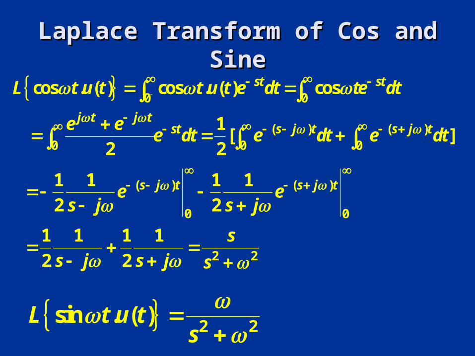
Laplace Transform of Cos and Laplace Transform of Cos and SineSine
0 0
( ) ( )0 0 0
( ) ( )
0 0
2 2
cos . ( ) cos . ( ) cos
1 [ ]
2 2
1 1 1 1
2 2
1 1 1 1
2 2
st st
j t j tst s j t s j t
s j t s j t
L t u t t u t e dt te dt
e ee dt e dt e dt
e es j s j
s
s j s j s
2 2sin . ( )L t u t
s
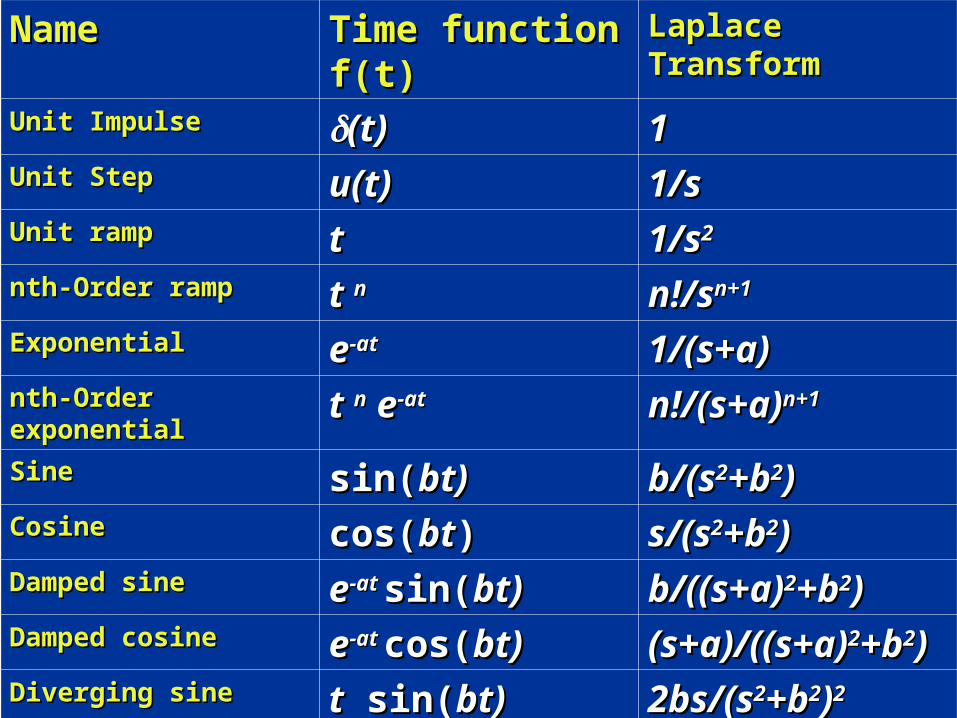
NameName Time function Time function f(t)f(t)
Laplace Laplace TransformTransform
Unit ImpulseUnit Impulse (t)(t) 11Unit StepUnit Step u(t)u(t) 1/s1/sUnit rampUnit ramp tt 1/s1/s22
nth-Order rampnth-Order ramp t t nn n!/sn!/sn+1n+1
ExponentialExponential ee-at-at 1/(s+a)1/(s+a)nth-Order nth-Order exponentialexponential
t t nn e e-at-at n!/(s+a)n!/(s+a)n+1n+1
SineSine sin(sin(bt)bt) b/(sb/(s22+b+b22))CosineCosine cos(cos(btbt)) s/(ss/(s22+b+b22))Damped sineDamped sine ee-at -at sin(sin(bt)bt) b/((s+a)b/((s+a)22+b+b22))Damped cosineDamped cosine ee-at -at cos(cos(bt)bt) (s+a)/(s+a)/
((s+a)((s+a)22+b+b22))Diverging sineDiverging sine tt sin( sin(bt)bt) 2bs/(s2bs/(s22+b+b22))22
Diverging cosineDiverging cosine tt cos( cos(bt)bt) (s(s22-b-b22)) /(s/(s22+b+b22))22
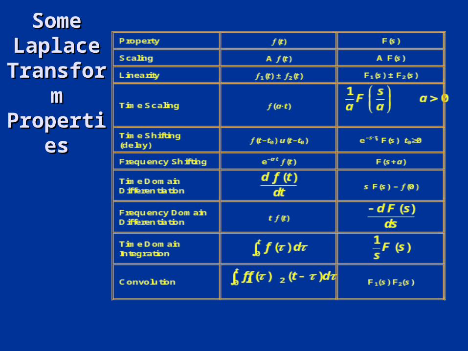
SomeSomeLaplace Laplace TransforTransfor
m m PropertiProperti
eses
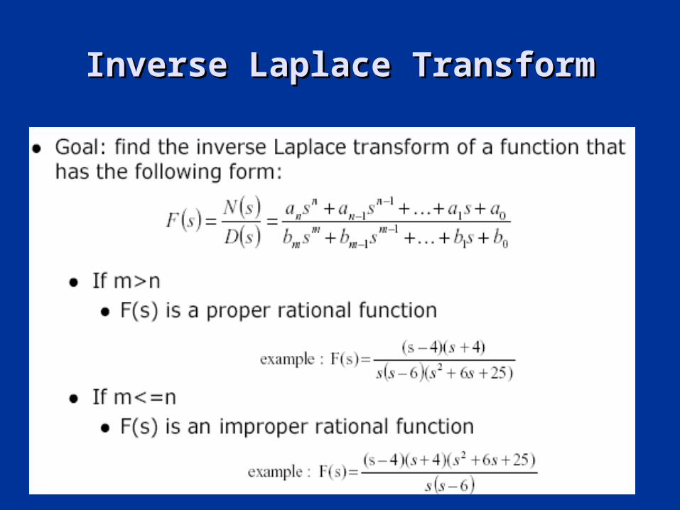
Inverse Laplace TransformInverse Laplace Transform
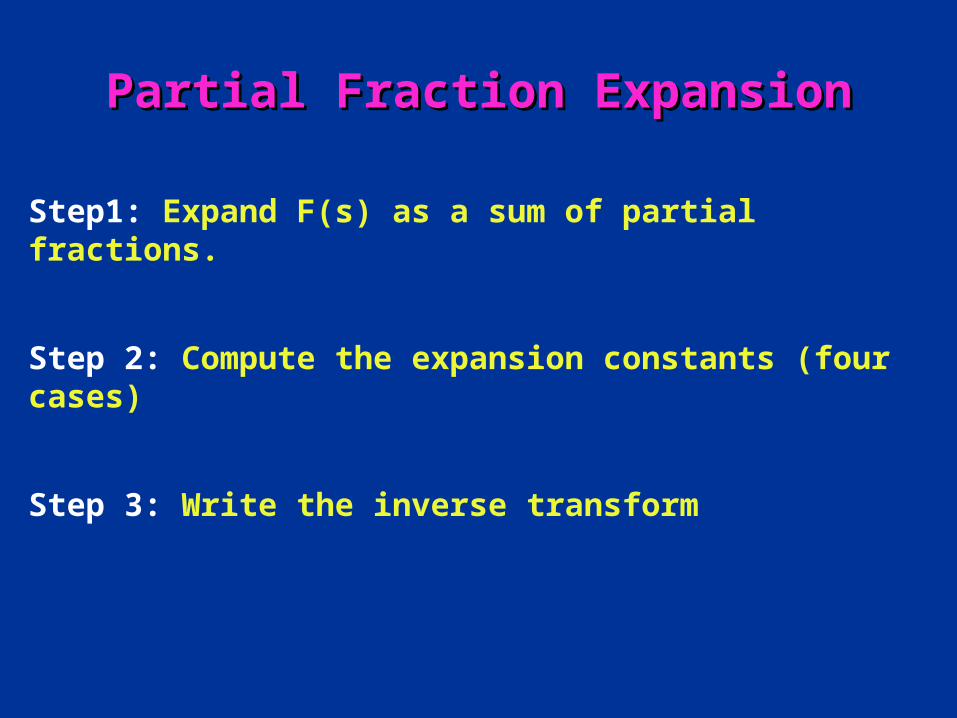
Partial Fraction ExpansionPartial Fraction Expansion
Step1: Expand F(s) as a sum of partial fractions.
Step 2: Compute the expansion constants (four cases)
Step 3: Write the inverse transform
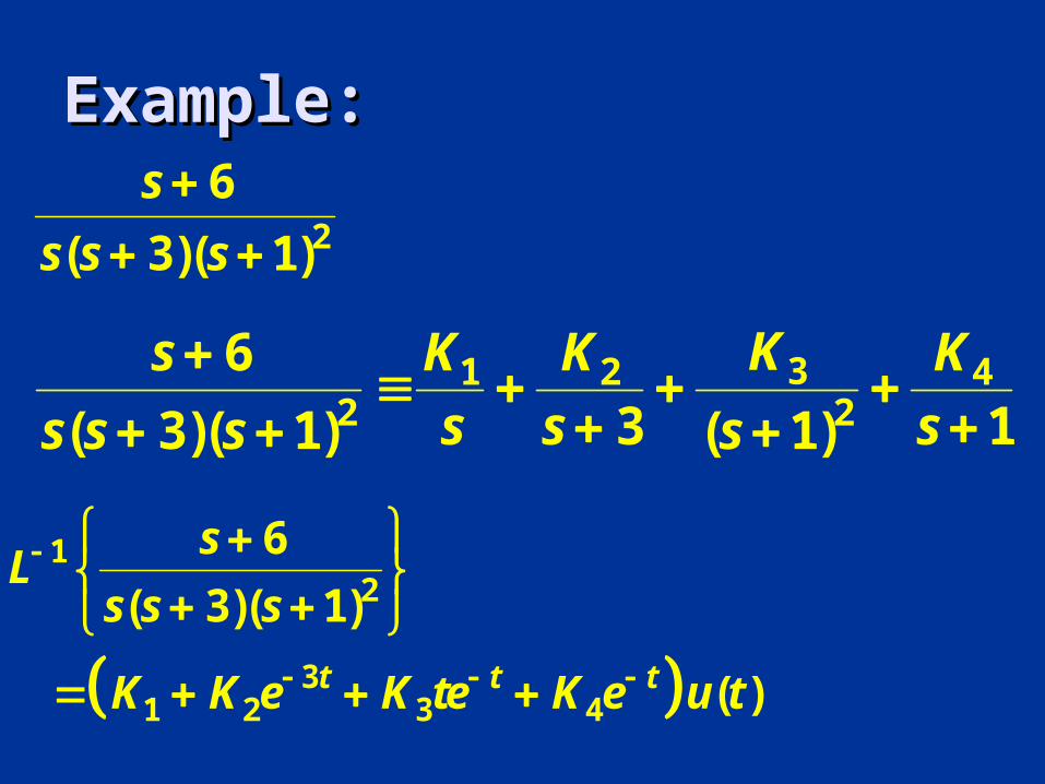
31 2 42 2
6
3 1( 3)( 1) ( 1)
KK K Ks
s s ss s s s
2
6
( 3)( 1)
s
s s s
12
31 2 3 4
6
( 3)( 1)
( )t t t
sL
s s s
K K e K te K e u t
Example:Example:
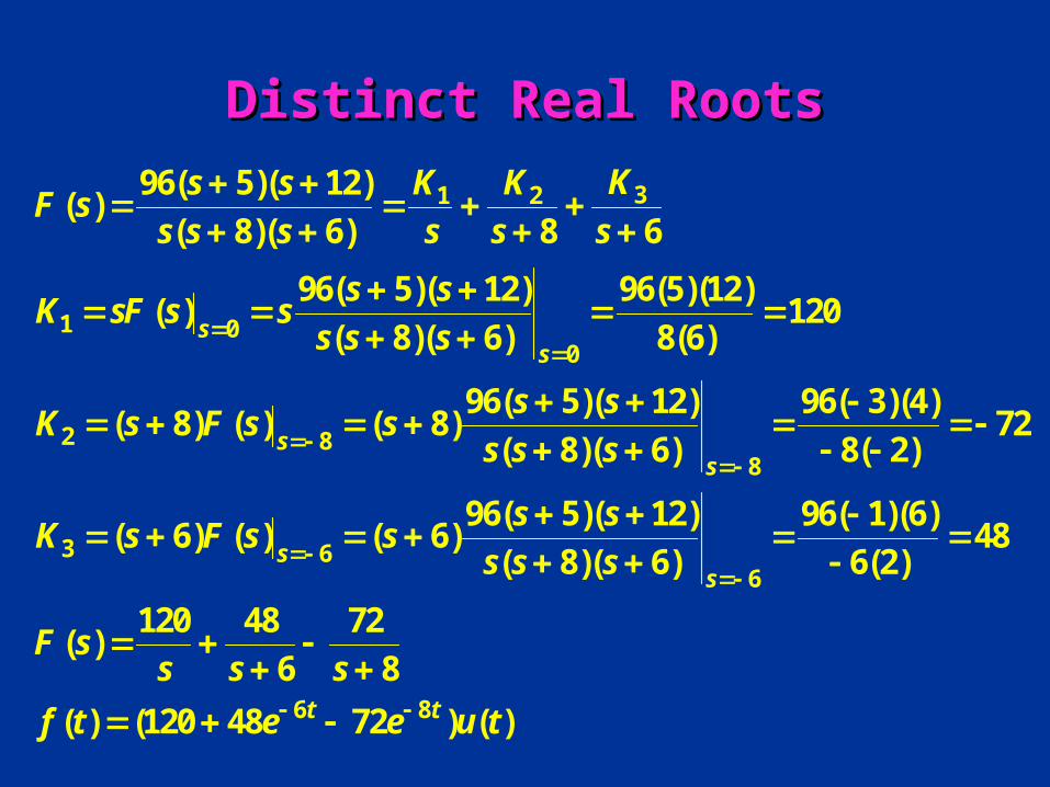
Distinct Real RootsDistinct Real Roots
31 2
1 00
2 88
3 6
96( 5)( 12)( )
( 8)( 6) 8 6
96( 5)( 12) 96(5)(12)( ) 120
( 8)( 6) 8(6)
96( 5)( 12) 96( 3)(4)( 8) ( ) ( 8) 72
( 8)( 6) 8( 2)
96(( 6) ( ) ( 6)
ss
ss
s
KK Ks sF s
s s s s s s
s sK sF s s
s s s
s sK s F s s
s s s
sK s F s s
6
6 8
5)( 12) 96( 1)(6)48
( 8)( 6) 6(2)
120 48 72( )
6 8
( ) (120 48 72 ) ( )
s
t t
s
s s s
F ss s s
f t e e u t
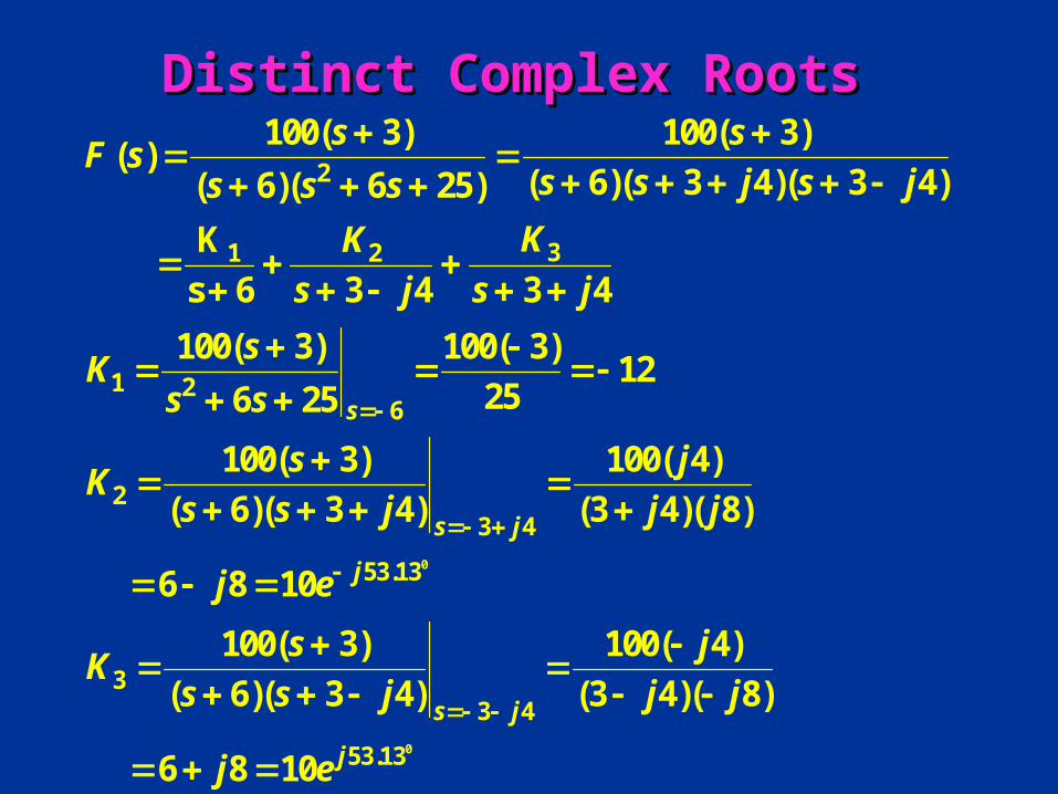
Distinct Complex RootsDistinct Complex Roots
0
2
31 2
1 26
23 4
53.13
3
100( 3) 100( 3)( )
( 6)( 3 4)( 3 4)( 6)( 6 25)
K
s 6 3 4 3 4
100( 3) 100( 3)12
256 25
100( 3) 100( 4)
( 6)( 3 4) (3 4)( 8)
6 8 10
1
s
s j
j
s sF s
s s j s js s s
KK
s j s j
sK
s s
s jK
s s j j j
j e
K
0
3 4
53.13
00( 3) 100( 4)
( 6)( 3 4) (3 4)( 8)
6 8 10
s j
j
s j
s s j j j
j e
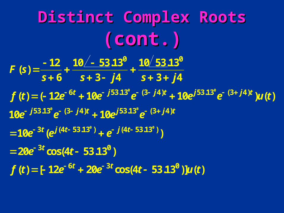
Distinct Complex RootsDistinct Complex Roots (cont.)(cont.)
0 0
0 0
0 0
0 0
6 53.13 (3 4) 53.13 (3 4)
53.13 (3 4) 53.13 (3 4)
3 (4 53.13 ) (4 53.13 )
3
12 10 53.13 10 53.13( )
6 3 4 3 4
( ) ( 12 10 10 ) ( )
10 10
10 ( )
20 cos(4 53.1
t j j t j j t
j j t j j t
t j t j t
t
F ss s j s j
f t e e e e e u t
e e e e
e e e
e t
0
6 3 0
3 )
( ) [ 12 20 cos(4 53.13 )] ( )t tf t e e t u t
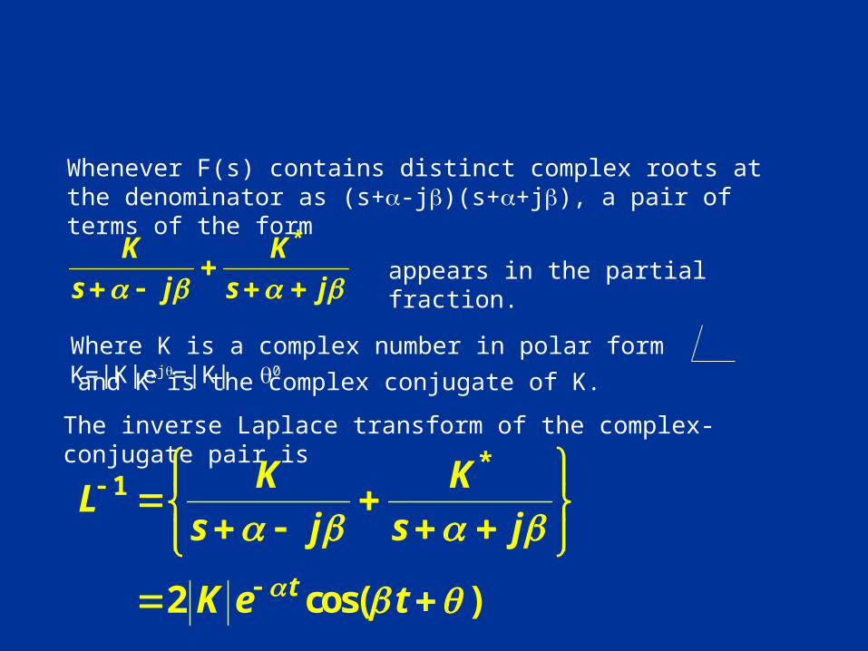
Whenever F(s) contains distinct complex roots at the denominator as (s+-j)(s++j), a pair of terms of the form *K K
s j s j
appears in the partial fraction.
Where K is a complex number in polar form K=|K|ej=|K| 0and K* is the complex conjugate of K.
The inverse Laplace transform of the complex-conjugate pair is *
1
2 cos( )t
K KL
s j s j
K e t
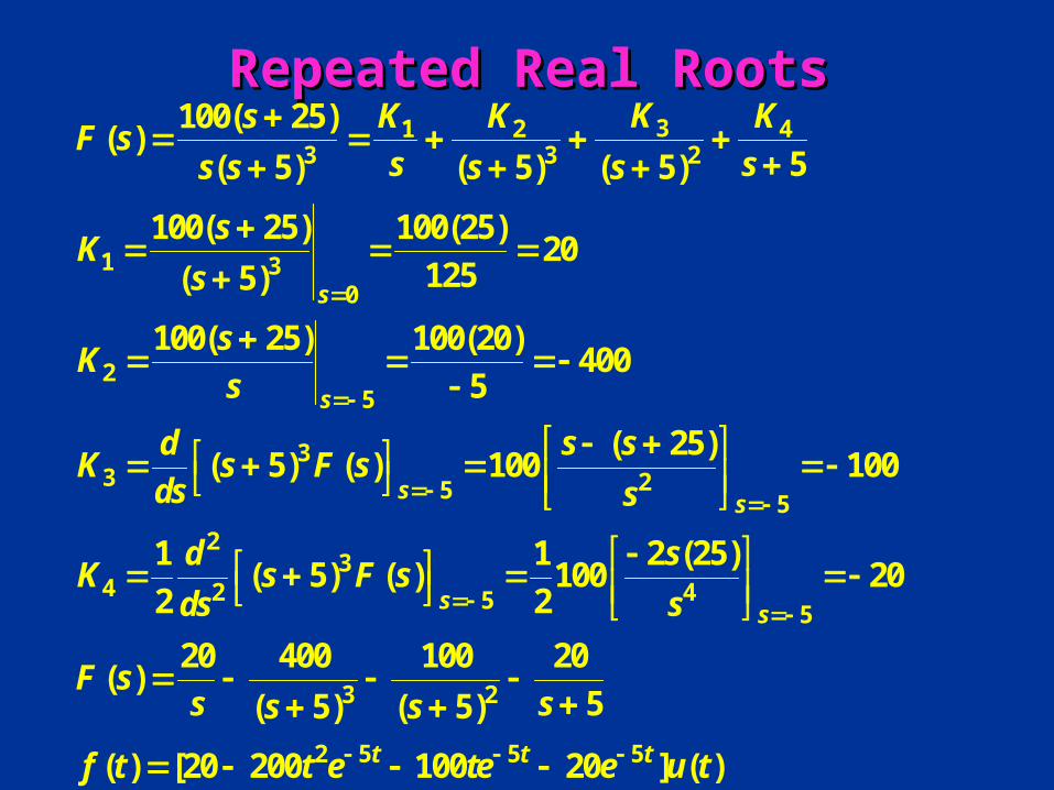
Repeated Real RootsRepeated Real Roots31 2 4
3 3 2
1 30
25
33 25
5
23
4 2 5
100( 25)( )
5( 5) ( 5) ( 5)
100( 25) 100(25)20
125( 5)
100( 25) 100(20)400
5
( 25)( 5) ( ) 100 100
1 1( 5) ( )
2 2
s
s
ss
s
KK K KsF s
s ss s s s
sK
s
sK
s
d s sK s F s
ds s
dK s F s
ds
45
3 2
2 5 5 5
2 (25)100 20
20 400 100 20( )
5( 5) ( 5)
( ) [20 200 100 20 ] ( )
s
t t t
s
s
F ss ss s
f t t e te e u t
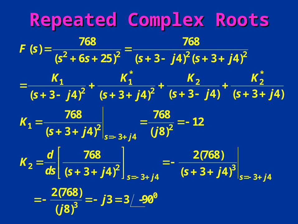
Repeated Complex RootsRepeated Complex Roots
2 2 2 2
* *1 1 2 2
2 2
1 2 23 4
2 2 33 4 3 4
3
768 768( )
( 6 25) ( 3 4) ( 3 4)
( 3 4) ( 3 4)( 3 4) ( 3 4)
768 76812
( 3 4) ( 8)
768 2(768)
( 3 4) ( 3 4)
2(768) 3
( 8)
s j
s j s j
F ss s s j s j
K K K K
s j s js j s j
Ks j j
dK
ds s j s j
jj
03 -90
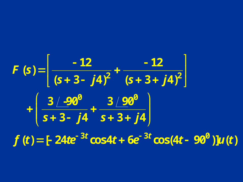
2 2
0 0
3 3 0
12 12( )
( 3 4) ( 3 4)
3 -90 3 90
3 4 3 4
( ) [ 24 cos4 6 cos(4 90 )] ( )t t
F ss j s j
s j s j
f t te t e t u t
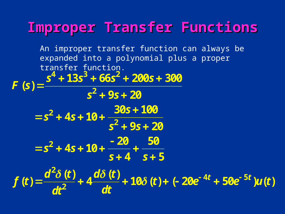
Improper Transfer FunctionsImproper Transfer FunctionsAn improper transfer function can always be expanded into a polynomial plus a proper transfer function.
4 3 2
2
22
2
24 5
2
13 66 200 300( )
9 2030 100
4 109 20
20 50 4 10
4 5
( ) ( )( ) 4 10 ( ) ( 20 50 ) ( )t t
s s s sF s
s ss
s ss s
s ss s
d t d tf t t e e u t
dtdt
POLES AND ZEROS OF F(s)POLES AND ZEROS OF F(s)
The rational function F(s) may be expressed as the ratio of two factored polynomials as
1 2
1 2
( )( ) ( )( )
( )( ) ( )n
m
K s z s z s zF s
s p s p s p
The roots of the denominator polynomial –p1, -p2, ..., -pm are called the poles of F(s). At these values of s, F(s) becomes infinitely large. The roots of the numerator polynomial -z1, -z2, ..., -zn are called the zeros of F(s). At these values of s, F(s) becomes zero.
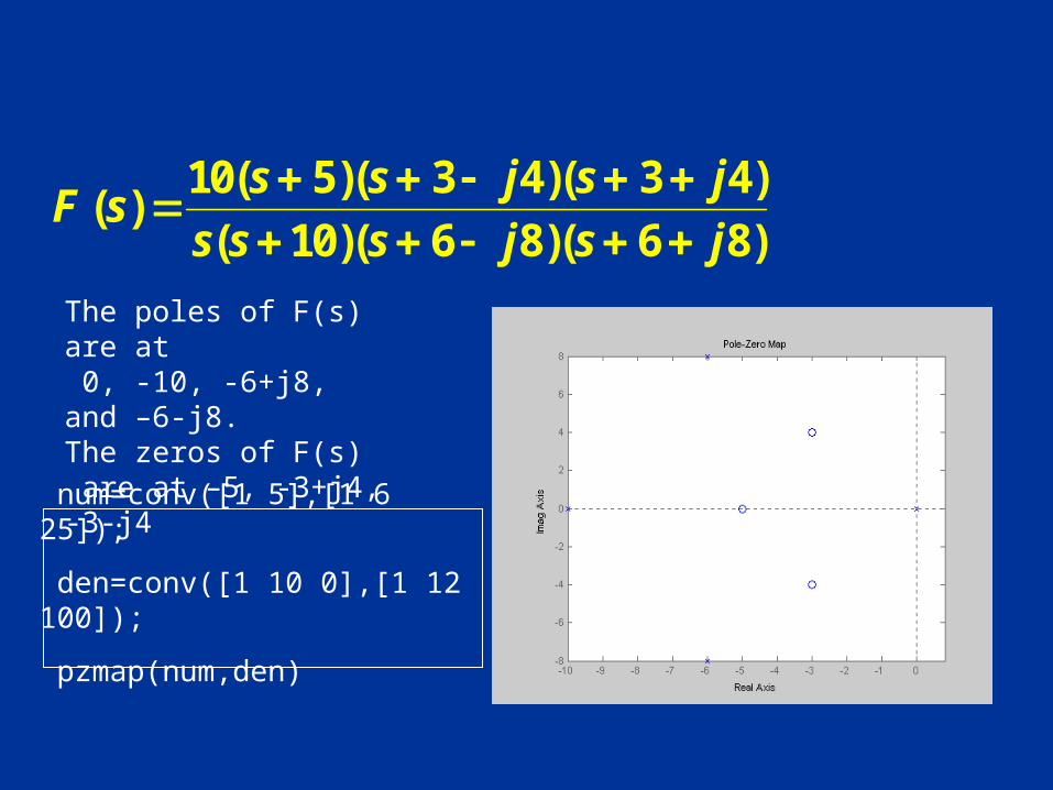
10( 5)( 3 4)( 3 4)( )
( 10)( 6 8)( 6 8)
s s j s jF s
s s s j s j
The poles of F(s) are at 0, -10, -6+j8, and –6-j8. The zeros of F(s) are at –5, -3+j4, -3-j4 num=conv([1 5],[1 6 25]);
den=conv([1 10 0],[1 12 100]);
pzmap(num,den)
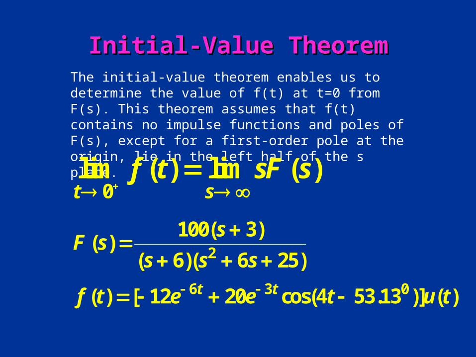
Initial-Value TheoremInitial-Value TheoremThe initial-value theorem enables us to determine the value of f(t) at t=0 from F(s). This theorem assumes that f(t) contains no impulse functions and poles of F(s), except for a first-order pole at the origin, lie in the left half of the s plane.
0lim ( ) lim ( )t s
f t sF s
2
6 3 0
100( 3)( )
( 6)( 6 25)
( ) [ 12 20 cos(4 53.13 )] ( )t t
sF s
s s s
f t e e t u t
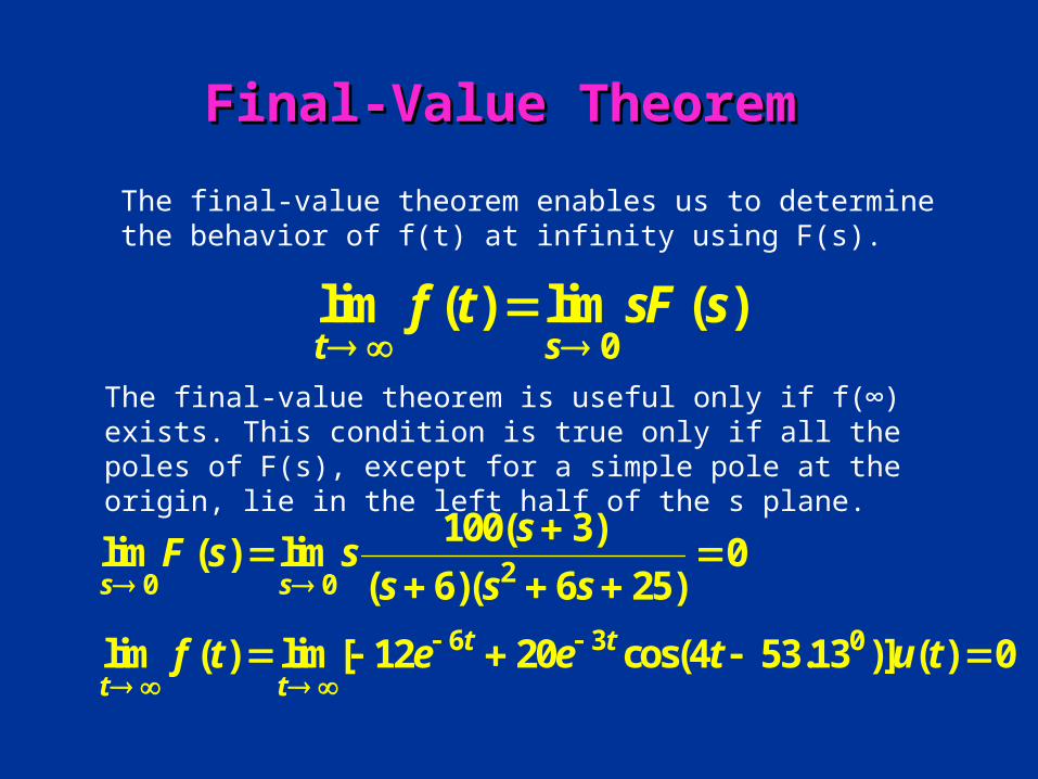
Final-Value TheoremFinal-Value Theorem
0lim ( ) lim ( )t s
f t sF s
The final-value theorem enables us to determine the behavior of f(t) at infinity using F(s).
The final-value theorem is useful only if f(∞) exists. This condition is true only if all the poles of F(s), except for a simple pole at the origin, lie in the left half of the s plane.
20 0
6 3 0
100( 3)lim ( ) lim 0
( 6)( 6 25)
lim ( ) lim[ 12 20 cos(4 53.13 )] ( ) 0
s s
t t
t t
sF s s
s s s
f t e e t u t