Introduction to kinetic models for biomass pyrolysis. Part 2.

Numerical techniques.

Gábor VárhegyiInstitute of Materials & Environmental Chemistry

Chemical Research CenterHungarian Academy of Sciences

2

Subtopics:

Can we evaluate the DTG curves instead of the TG curveswithout introducing mathematical errors/artifacts? (How to getreliable DTG?)

What numerical methods are well worth to use in the solution of the kinetic equations and in the minimization of the least squares sum?

3

Determination of the DTG curve (1)If the errors are random, we can estimate the noise level of a given

curve by simple statistical checks, then we can find a “smooth” f(t) function approximating the experimental data within the given noise level:

average smoothness of f(t) ≈ maximum (1) N

Σ wi2 (f(ti)–Xi)2 ≤ N σ2 (2)

i=1

Here N, f(t), t, Xi and σ denote the number of data, the smoothing function, the time, the observations, and the noise level, respectively. The use of weight factors wi is optional. (We can use wi≡1 values). This type of smoothing was invented by Whittaker & Robinson more then 70 years ago! (Their book, The Calculus of Observations is a treasure for science history.) Later Reinsch developed an effective algorithm for the calculation of cubic spline functions satisfying conditions (1) – (2). This method is now part of every major mathematical program library.

4

Determination of the DTG curve (2)

The noise level can be estimated by simple statistical checks. The smoothing of the random noise, however, is not

enough due to wave-like errors! We must increase σ gradually till we got an acceptable compromise.

For example, let us suppose that the random noise is 0.3µg and we get the acceptable compromise at 0.5 µg. Then the systematic error is not higher than 0.2 µg. It is surely negligible at a sample mass of 2 mg and acceptable at a sample mass of 0.2 mg.

If the TG system is in a good shape and carefully cleaned from tar deposits, etc., even better values can be achieved, as the following examples show.

5

Determination of the DTG curve: Smoothing a the statistic noise

100 200 300 400 500 °C0.0

0.1

0.2

0.3

0.4

0.5

mg

0.0

0.2

0.4

0.6

0.8

ug/s

Corn cob charcoal 03.12.31, middle section, Ø 10.6 µm (10 min grinding) m0= 0.613 mg, O2: 140 ml/min, 5 °C/min Spline DTG: actual deviation of G = .056 microgram DTGmax: 1.694E-01%/s ( 1.035E-03 mg/s) at 415.0°C

6

Determination of the DTG curve: Smoothing more than the statistic noise

100 200 300 400 500 °C0.0

0.1

0.2

0.3

0.4

0.5

mg

0.0

0.2

0.4

0.6

0.8

ug/s

Corn cob charcoal 03.12.31, middle section, Ø 10.6 µm (10 min grinding) m0= 0.613 mg, O2: 140 ml/min, 5 °C/min Spline DTG: actual deviation of G = .086 microgram DTGmax: 1.623E-01%/s ( 1.034E-03 mg/s) at 414.8°C

7Time (min)

Inte

nsity

(co

unts

/s)

0 10 20 30 40 50 60 70

Sample T237m/z 15 (CH3

+) unprocessed signal

1015202530354045505560 Example from

TGA-MS experiments

8Time (min)

Inte

nsity

(co

unts

/s)

0 10 20 30 40 50 60 70

Sample T237m/z 15 (CH3

+) unprocessed signal smoothing spline

1015202530354045505560 Example from

TGA-MS experiments

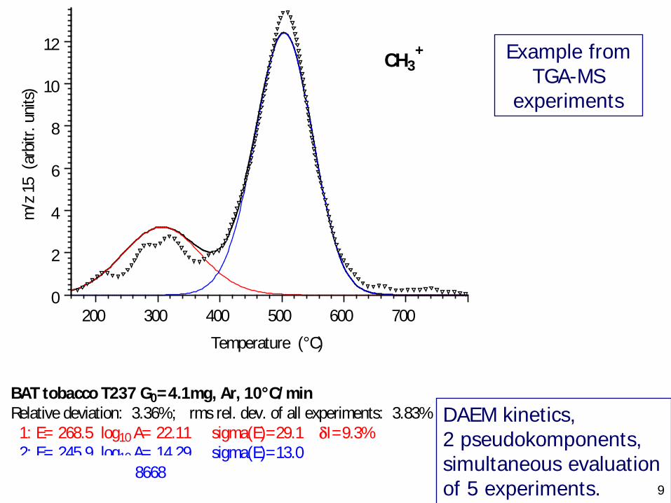
9

DAEM kinetics,2 pseudokomponents, simultaneous evaluation of 5 experiments.

Temperature (°C)

m/z

15

(arb

itr. u

nits

)

200 300 400 500 600 700

CH3+

0

2

4

6

8

10

12

BAT tobacco T237 G0=4.1mg, Ar, 10°C/minRelative deviation: 3.36%; rms rel. dev. of all experiments: 3.83% 1: E= 268.5 log10 A= 22.11 sigma(E)=29.1 δI=9.3% 2: E= 245.9 log10 A= 14.29 sigma(E)=13.0C: 3004 8668

Example from TGA-MS

experiments

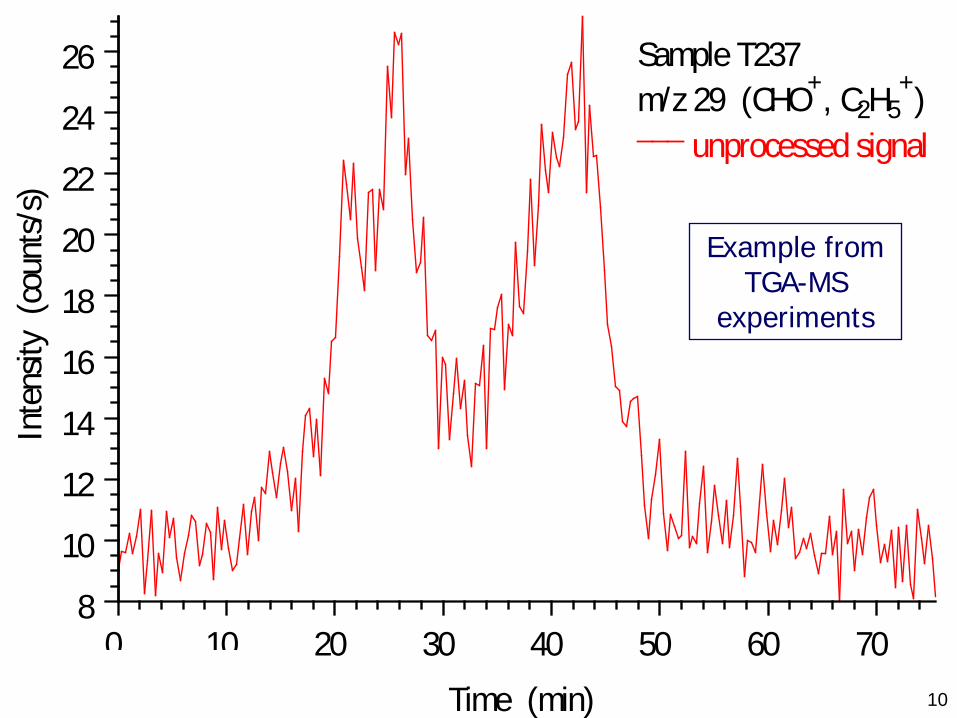
10Time (min)

Inte

nsity

(co

unts

/s)

0 10 20 30 40 50 60 70

Sample T237m/z 29 (CHO+, C2H5

+) unprocessed signal

8

10

12

14

16

18

20

22

24

26

Example from TGA-MS

experiments

11Time (min)

Inte

nsity

(co

unts

/s)

0 10 20 30 40 50 60 70

Sample T237m/z 29 (CHO+, C2H5

+) unprocessed signal smoothing spline

8

10

12

14

16

18

20

22

24

26

Example from TGA-MS

experiments

12

Temperature (°C)

m/z

29

(arb

itr. u

nits

)

200 300 400 500 600

CHO+, C2H5+

0

1

2

3

BAT tobacco T237 G0=4.1mg, Ar, 10°C/minRelative deviation: 8.12%; rms rel. dev. of all experiments: 6.45% 1: E= 222.6 log10 A= 18.03 sigma(E)=16.3 δI=-1.9% 2: E= 259.4 log10 A= 16.02 sigma(E)=14.8C: 2362 2387

DAEM kinetics,2 pseudokomponents, simultaneous evaluation of 5 experiments.

Example from TGA-MS

experiments

13

Methods for a general least squares process:

I. Basic considerations:

The time of the programmers is much more expensive than the time ofthe computer.

An ordinary desktop PC in the order of € 400 can do the job. Sinceinvention of the ~3 GHz processors, simple runs take only seconds.Nowadays the longest runs take less than a night (unattended) or a day(as a low priority background job). 15 years ago the evaluation of ahuge data set by a complex model required 1 month. During a longerrun, the program saves the results in every 15 minutes automatically.(No problem with blackouts, if any. Besides, we can survey after anunattended run what happened, how the optimum was found).

The complexity of the programs should be kept within limits, otherwisewe cannot modify them for different tasks / mechanisms / evaluationstrategies.

Accordingly, simple, but safe techniques should be selected.

14

Methods for a general least squares process II. ODE solutionPart 1: Independent 1st order reactions:

The solution of the 1st order kinetic equation can be carried out via a simple, fast integration at any T(t).

Let us separate the variables and integrate both sides:

dα/dt = k(T) (1-α)

dα/(1-α) = k(T) dt

∫ (1-α)-1 dα = ∫ k(T) dt

The left hand side is the logarithm function, the right-hand side can be easily integrated numerically by well-known methods to any precision ...

This is applicable if a biomass is described by assuming independent, parallel reactions. Cannot be employed, however, for successive and/or competitive reactions; in such cases a general ODE solving algorithm is more straightforward.

15

Methods for a general least squares process II. ODE solution

Part 2. Solution of a general system of ordinary differential equations:One of the simplest methods is the Runge Kutta family of ODE solvers.If the step size is continuously adjusted, it can safely keep any reasonableprecision. (Except in the case of a stiff system of ODEs!). I usually set aprecision of 10-8, and refine the results with another run of the evaluationsoftware with a precision of 10-10. Why to use such tight precisionrequirements?(Just to be absolutely sure that the found optimum is not affected bymathematical artifacts. It’s free!)

One could hope larger step sizes by a more advanced technique.But can a step size by higher than the step size of the observations?

No! We measure discrete temperature values. In my programs, the T(t)functions are constructed by simple interpolation. One could use splineapproximations, too. In both cases, however, either T(t) or its derivatives arenot smooth in the points of the observations. Accordingly, we can solve theODEs separately, in each intervals:[t1, t2], [t2, t3], [t3, t4], ...

16

Methods for a general least squares process:

III. Optimization:Which is a simple, but safe method?Should we bother with finding analytical or numerical derivatives?

In the fifties, discrete steps were made in each direction, successively:

17

Methods for a general least squares process III. Optimization

Later, in 1961, Hook and Jeeves added a step in the direction of the valley found in each cycle (see the red arrows in the figure.)

This invention improved the speed. This simple algorithm is very stable and finds a minimum at any topography. [See the recent results of Torczon et al.] Contrary to the Simplex method of Nelder and Mead: the simplex sometime flatten, and one dimension is loss. One can easily supplement this method by refining the step-length by parabolic interpolation/extrapolation in each step. (Its result is used only when it is significantly better than the unrefined step.)

18

Methods for a general least squares process III. Optimization

Further advantages of the Hook – Jeeves method:

(1) Works simple and safely in the case of interval bonds on the variables, e.g.: 0 ≤ n ≥ 3; 30 ≤ E ≤ 300

(2) In our case, several parameters affect only one ODE in the system. For example, if we evaluate a series of experiments with common E, while each experiment has its own ln A and m∞ then each ln A and m∞ affect only one ODE. In the steps in the direction of these parameters only one ODE should be solved.

19

Methods for a general least squares process V. Separation of the linear and non-linear parameters

∑=

=−M

jjj dtdcdtdm

1// α

( ) ( )[ ] min2

1 12 =

−=∑∑

= =

N

k

N

i kk

icalcki

obsk

N

k

hNtXtXS

SN is quadratic for parameters cj. They can be obtained by solving a system of linear equation by any set of Ej and Aj. Accordingly, only Ej and Aj should be searched by a general minimization algorithm.

Safety considerations: Whatever combinations arise temporarily during the minimization of SN, the algorithm must not go astray. Accordingly, the program should automatically employ some strategy (e.g. a Tikhanov's regularization) for finding meaningful parameters if it observes ill-definition. Besides, the program must not allow negative cj (except if the user explicitly tells such exception at the very beginning of the run).

20

Methods for a general least squares process VI. Parameter transformations

The parameters can compensate each other so some extent. For examplea change of E can be counterbalanced more or less by a proper change ofA. Many authors believed deeper physical content behind this simplemathematical consequence that can be deduced easily from the propertiesof the Arrhenius type equations at non-isothermal T(t) programs.

The compensation effects can slow down the evaluation. One can fightagainst them by simple parameter transformations that decrease thedependence between the unknown parameters.

Nowadays I am not sure that such transformations are important, except asimple and trivial one:

ln A or log10 A should be used instead of A

to avoid unpleasant geometries. Try to visualize an Arrhenius equation inthe following way:

k(T) = exp( ln A – E/RT )

21

End of these lectures.Thanks for your attention. See you tomorrow!