Introduction to Growth Modeling in Mplus...curve modeling. Growth Modeling in Mplus ... The...
99
Growth Modeling in Mplus Introduction to Growth Modeling in Mplus Xin Feng, Ph.D. Department of Human Sciences Human Development & Family Science Program
Transcript of Introduction to Growth Modeling in Mplus...curve modeling. Growth Modeling in Mplus ... The...

Growth Modeling in Mplus
Introduction to Growth Modeling in Mplus
Xin Feng, Ph.D.
Department of Human Sciences
Human Development & Family Science Program
Growth Modeling in Mplus
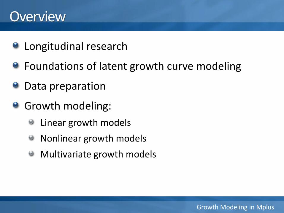
Overview
Longitudinal research
Foundations of latent growth curve modeling
Data preparation
Growth modeling:
Linear growth models
Nonlinear growth models
Multivariate growth models
Growth Modeling in Mplus
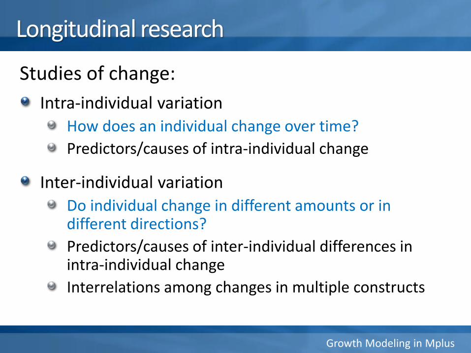
Longitudinal research
Studies of change:
Intra-individual variationHow does an individual change over time?
Predictors/causes of intra-individual change
Inter-individual variationDo individual change in different amounts or in different directions?
Predictors/causes of inter-individual differences in intra-individual change
Interrelations among changes in multiple constructs

Growth Modeling in Mplus
Features of a longitudinal study
Multiple waves of data (repeated measures)Same individuals measured at different times
Change as a process vs. an increment
An outcome that change systematically over time
Measures with good psychometric properties
Longitudinal equivalence of the scores
A sensible metric of time
Growth Modeling in Mplus
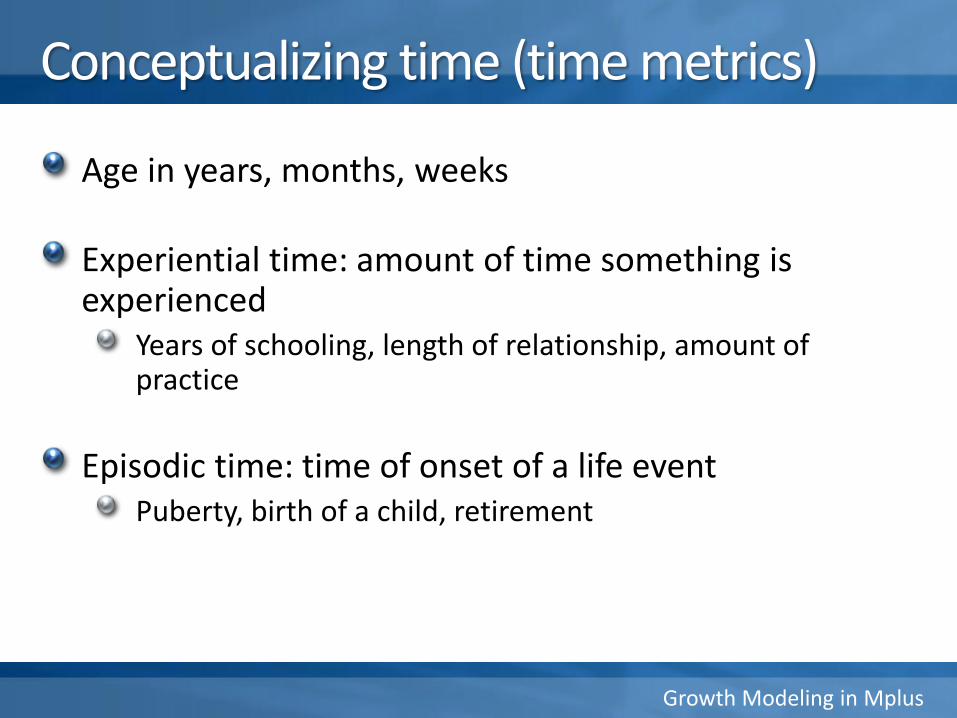
Conceptualizing time (time metrics)
Age in years, months, weeks
Experiential time: amount of time something is experienced
Years of schooling, length of relationship, amount of practice
Episodic time: time of onset of a life eventPuberty, birth of a child, retirement
Growth Modeling in Mplus
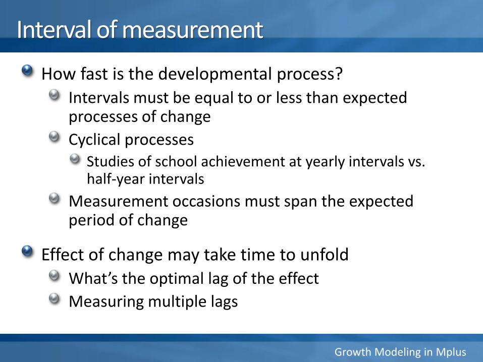
Interval of measurement
How fast is the developmental process?Intervals must be equal to or less than expected processes of change
Cyclical processesStudies of school achievement at yearly intervals vs. half-year intervals
Measurement occasions must span the expected period of change
Effect of change may take time to unfoldWhat’s the optimal lag of the effect
Measuring multiple lags
Growth Modeling in Mplus
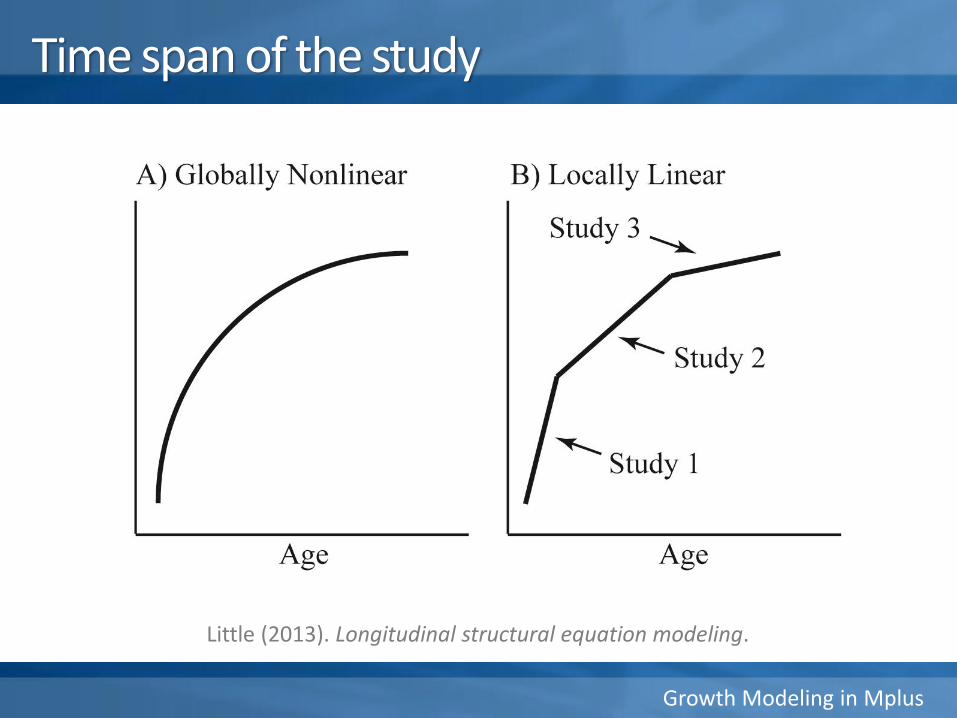
Little (2013). Longitudinal structural equation modeling.
Time span of the study
Growth Modeling in Mplus
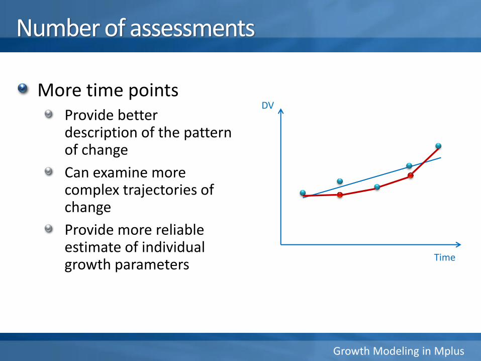
Number of assessments
More time points Provide better description of the pattern of change
Can examine more complex trajectories of change
Provide more reliable estimate of individual growth parameters
DV
Time
Growth Modeling in Mplus
A conceptual framework for longitudinal research
Longitudinal research involves:
A theoretical model of change
A design that can capture the process of change
A statistical model that tests the theoretical model
Growth Modeling in Mplus
Foundations of latent growth curve modeling

Growth Modeling in Mplus
Individual change over time
30
35
40
45
1 2 3 4 5 6
y
t
The intercept The slope
3i 4i
5i
1i
6i
titiiitiy 10

Growth Modeling in Mplus
t
y
titiiitiy 10
iii
iii
rx
rx
111101
001000
Growth Modeling in Mplus
Latent growth models
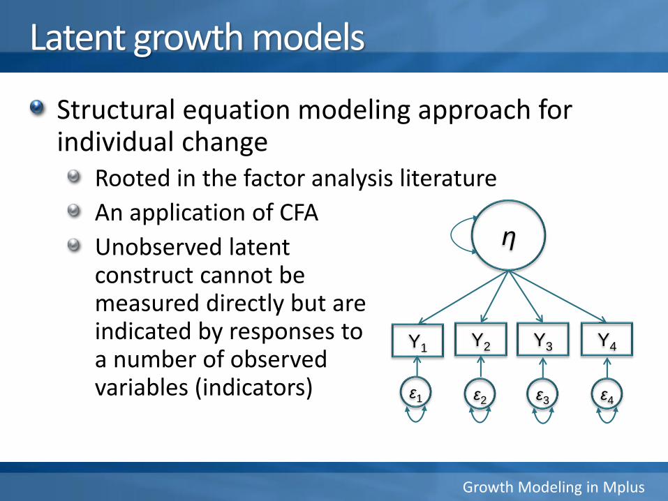
Structural equation modeling approach for individual change
Rooted in the factor analysis literature
An application of CFA
Unobserved latent construct cannot be measured directly but are indicated by responses to a number of observed variables (indicators)
η
Y1Y2 Y3
ε1 ε2 ε3
Y4
ε4
Growth Modeling in Mplus
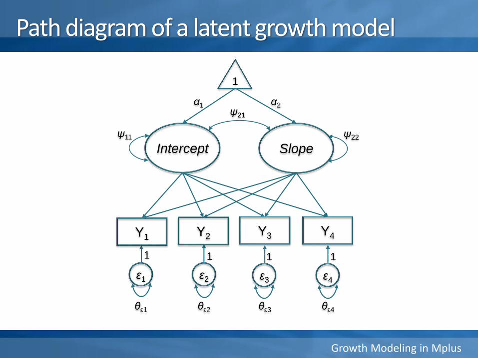
Path diagram of a latent growth model
ψ21
Slope
ψ22
1
α1 α2
Intercept
Y1 Y2 Y3
ε1 ε2 ε3
Y4
ε4
1 1 1 1
ψ11
θε1 θε2 θε3 θε4
Growth Modeling in Mplus
Latent growth models
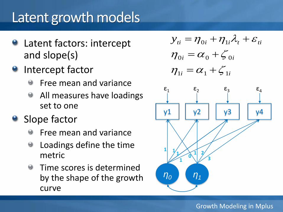
Latent factors: intercept and slope(s)
Intercept factorFree mean and variance
All measures have loadings set to one
Slope factor Free mean and variance
Loadings define the time metric
Time scores is determined by the shape of the growth curve
y1 y2 y3 y4
η0 η1
ε1 ε2 ε3 ε4
ii
ii
111
000
titiitiy 10
1 11
10
1 23
Growth Modeling in Mplus
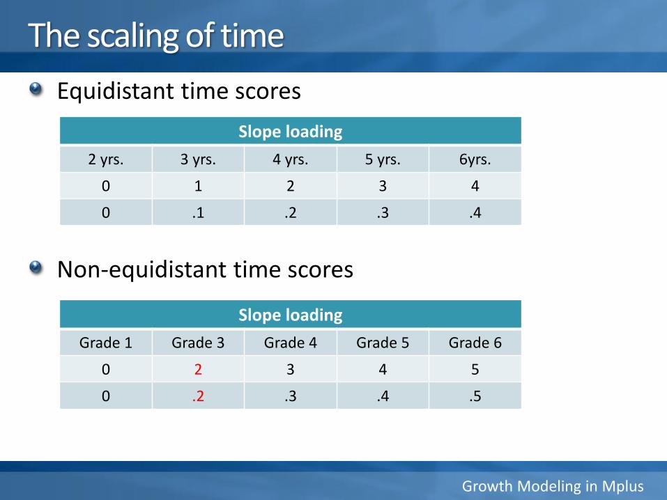
The scaling of time
Equidistant time scores
Non-equidistant time scores
Slope loading
2 yrs. 3 yrs. 4 yrs. 5 yrs. 6yrs.
0 1 2 3 4
0 .1 .2 .3 .4
Slope loading
Grade 1 Grade 3 Grade 4 Grade 5 Grade 6
0 2 3 4 5
0 .2 .3 .4 .5
Growth Modeling in Mplus
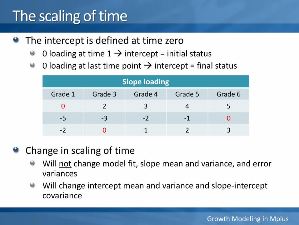
The scaling of time
The intercept is defined at time zero0 loading at time 1 intercept = initial status
0 loading at last time point intercept = final status
Change in scaling of time Will not change model fit, slope mean and variance, and error variances
Will change intercept mean and variance and slope-intercept covariance
Slope loading
Grade 1 Grade 3 Grade 4 Grade 5 Grade 6
0 2 3 4 5
-5 -3 -2 -1 0
-2 0 1 2 3
Growth Modeling in Mplus
Linear growth factors
For both the intercept and slope growth factors there is a mean and a variance
Intercept (initial status)
Mean
Average of the outcome across individual at the time point where the time score is zero
When the first time score is zero, it represent the initial status
Variance
how much individuals differ in their intercepts
Growth Modeling in Mplus
Linear slopeMean: average growth rate across individuals
Variance: individual variation of the growth rate
Covariance between intercept and slope
Outcome (observed variable) parametersIntercepts: fixed at zero (not estimated)
Residual variance: time specific and measurement error variance
Residual covariance: relations between time-specific and measurement error variation across time
Growth Modeling in Mplus
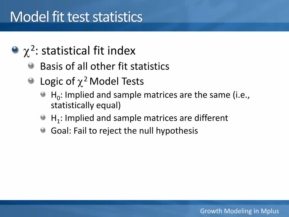
Model fit test statistics
2: statistical fit indexBasis of all other fit statistics
Logic of 2 Model TestsH0: Implied and sample matrices are the same (i.e., statistically equal)
H1: Implied and sample matrices are different
Goal: Fail to reject the null hypothesis
Growth Modeling in Mplus
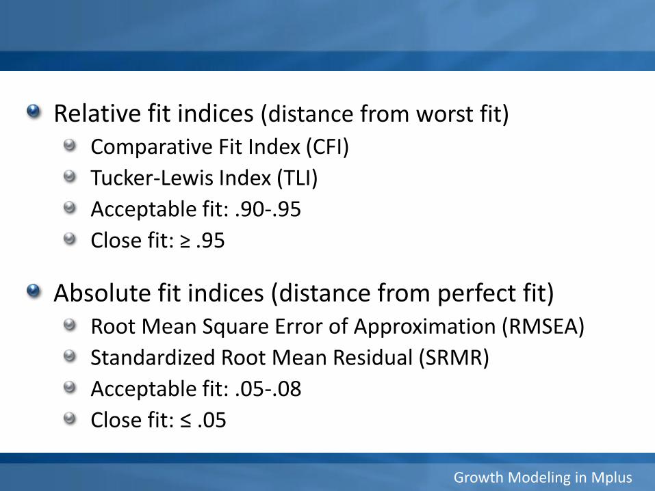
Relative fit indices (distance from worst fit)
Comparative Fit Index (CFI)
Tucker-Lewis Index (TLI)
Acceptable fit: .90-.95
Close fit: ≥ .95
Absolute fit indices (distance from perfect fit) Root Mean Square Error of Approximation (RMSEA)
Standardized Root Mean Residual (SRMR)
Acceptable fit: .05-.08
Close fit: ≤ .05
Growth Modeling in Mplus
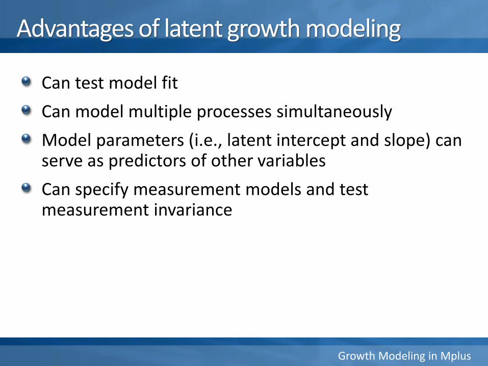
Advantages of latent growth modeling
Can test model fit
Can model multiple processes simultaneously
Model parameters (i.e., latent intercept and slope) can serve as predictors of other variables
Can specify measurement models and test measurement invariance

Growth Modeling in Mplus
Data preparation
Growth Modeling in Mplus
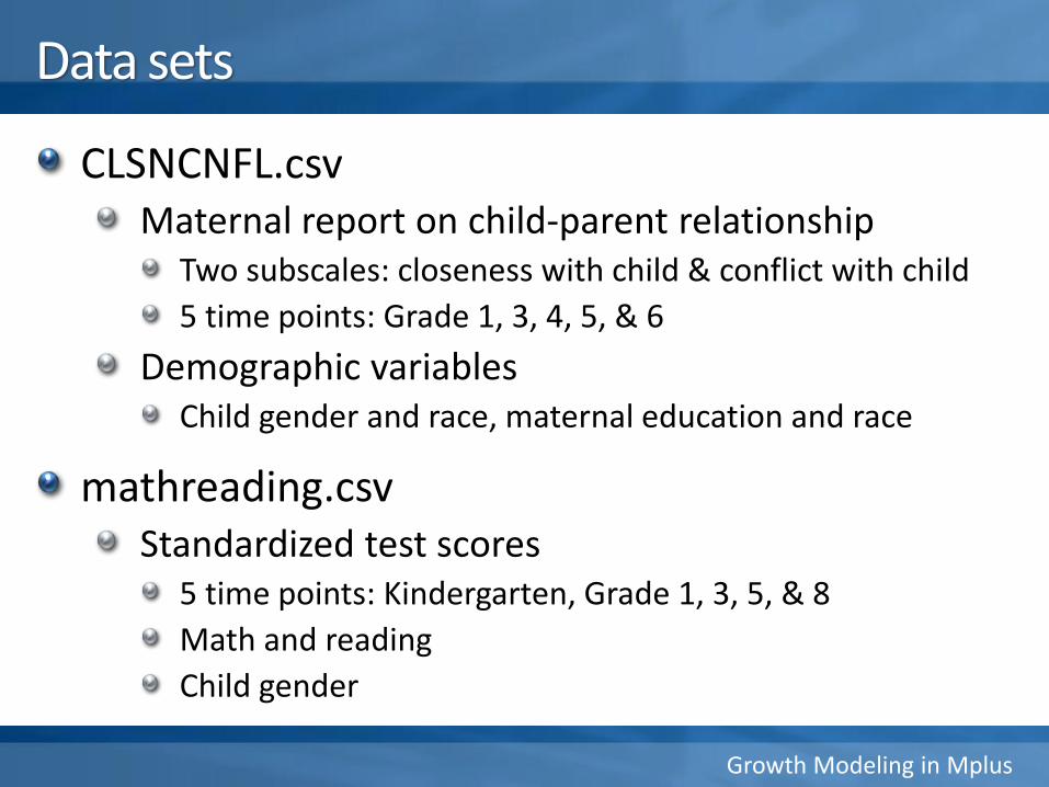
Data sets
CLSNCNFL.csvMaternal report on child-parent relationship
Two subscales: closeness with child & conflict with child
5 time points: Grade 1, 3, 4, 5, & 6
Demographic variablesChild gender and race, maternal education and race
mathreading.csvStandardized test scores
5 time points: Kindergarten, Grade 1, 3, 5, & 8
Math and reading
Child gender
Growth Modeling in Mplus
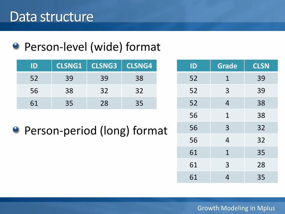
Data structure
Person-level (wide) format
Person-period (long) format
ID CLSNG1 CLSNG3 CLSNG4
52 39 39 38
56 38 32 32
61 35 28 35
ID Grade CLSN
52 1 39
52 3 39
52 4 38
56 1 38
56 3 32
56 4 32
61 1 35
61 3 28
61 4 35
Growth Modeling in Mplus
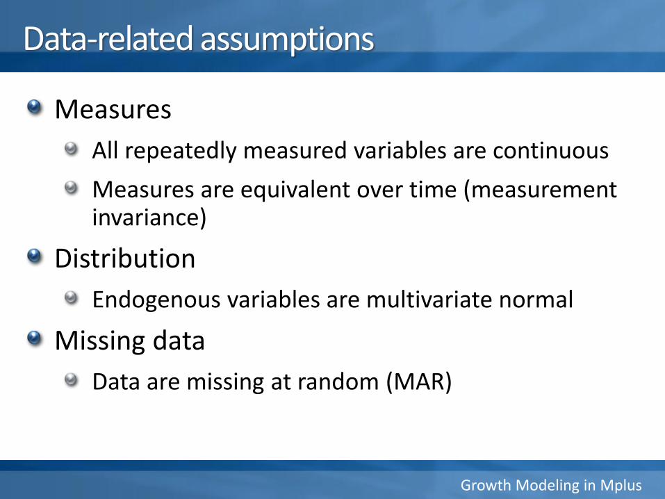
Data-related assumptions
Measures
All repeatedly measured variables are continuous
Measures are equivalent over time (measurement invariance)
Distribution
Endogenous variables are multivariate normal
Missing data
Data are missing at random (MAR)
Growth Modeling in Mplus
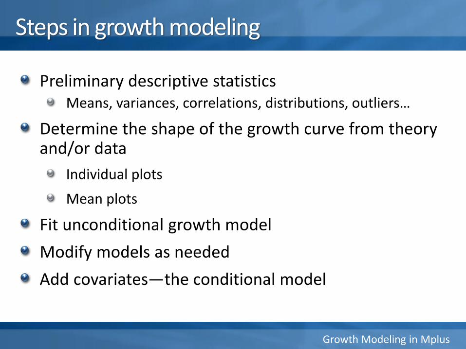
Steps in growth modeling
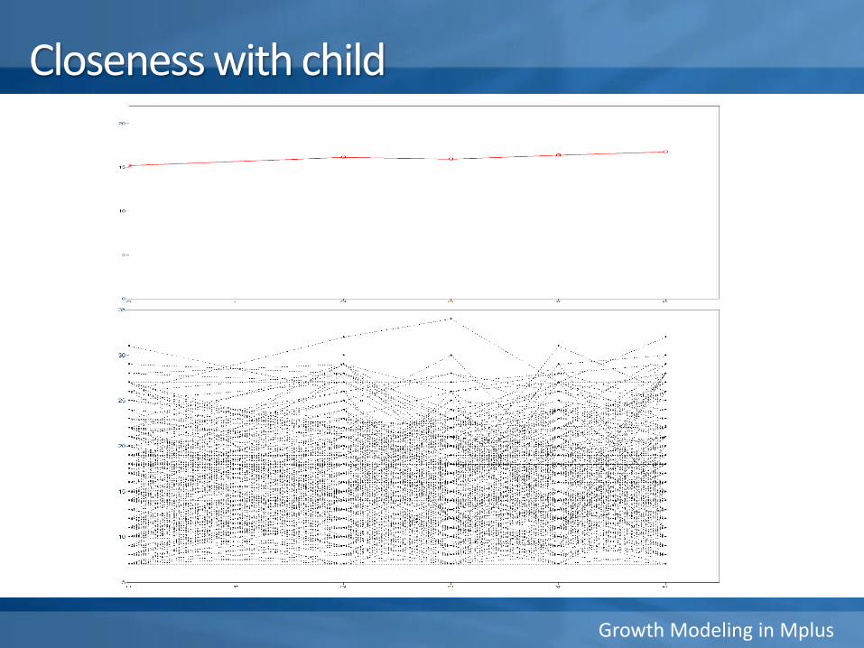
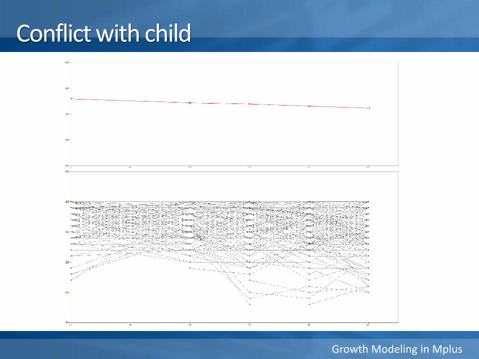
Preliminary descriptive statisticsMeans, variances, correlations, distributions, outliers…
Determine the shape of the growth curve from theory and/or data
Individual plots
Mean plots
Fit unconditional growth model
Modify models as needed
Add covariates—the conditional model
Growth Modeling in Mplus
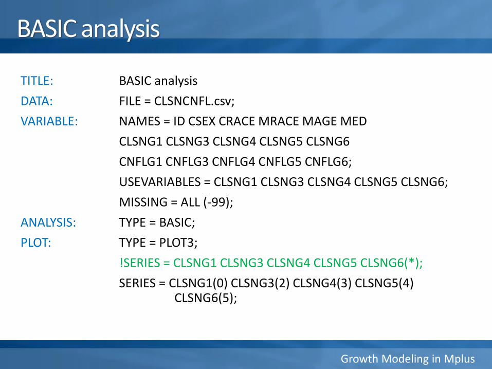
BASIC analysis
TITLE: BASIC analysis
DATA: FILE = CLSNCNFL.csv;
VARIABLE: NAMES = ID CSEX CRACE MRACE MAGE MED
CLSNG1 CLSNG3 CLSNG4 CLSNG5 CLSNG6
CNFLG1 CNFLG3 CNFLG4 CNFLG5 CNFLG6;
USEVARIABLES = CLSNG1 CLSNG3 CLSNG4 CLSNG5 CLSNG6;
MISSING = ALL (-99);
ANALYSIS: TYPE = BASIC;
PLOT: TYPE = PLOT3;
!SERIES = CLSNG1 CLSNG3 CLSNG4 CLSNG5 CLSNG6(*);
SERIES = CLSNG1(0) CLSNG3(2) CLSNG4(3) CLSNG5(4) CLSNG6(5);
Growth Modeling in Mplus
Closeness with child
Growth Modeling in Mplus
Conflict with child
Growth Modeling in Mplus
Run the BASIC analysis for mathK-mathG8, using the mathreading.csv data set

Growth Modeling in Mplus
Unconditional growth model – Linear growth

Growth Modeling in Mplus
Mplus language
y1 y2 y3 y4
i s
ε1 ε2 ε3 ε4
MODEL:
i s| y1@0 y2@1 y3@2 y4@3;
! Alternative language;
MODEL:
i BY y1-y4@1
s BY y1@0 y2@1 y3@2 y4@3;
[y1-y4@0]; !Fix the intercepts of y1-y4 at 0;
[i s]; !Freely estimate the latent means of intercept & slope;
Growth Modeling in Mplus
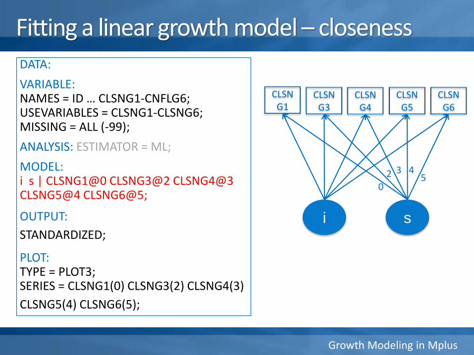
Fitting a linear growth model – closenessDATA:
VARIABLE:NAMES = ID … CLSNG1-CNFLG6;USEVARIABLES = CLSNG1-CLSNG6;MISSING = ALL (-99);
ANALYSIS: ESTIMATOR = ML;
MODEL:i s | CLSNG1@0 CLSNG3@2 CLSNG4@3 CLSNG5@4 CLSNG6@5;
OUTPUT:
STANDARDIZED;
PLOT:TYPE = PLOT3;SERIES = CLSNG1(0) CLSNG3(2) CLSNG4(3)
CLSNG5(4) CLSNG6(5);
CLSN G1
CLSN G4
CLSN G5
CLSN G6
i s
CLSN G3
02 3 4
5

Growth Modeling in Mplus
Sample and estimated means – closeness
Growth Modeling in Mplus
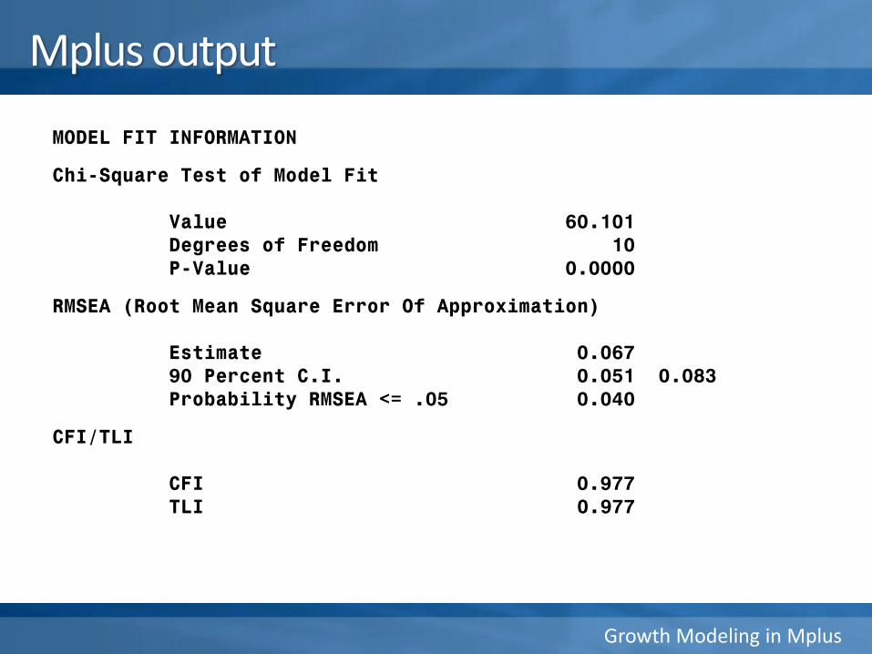
MODEL FIT INFORMATION
Chi-Square Test of Model Fit
Value 60.101Degrees of Freedom 10P-Value 0.0000
RMSEA (Root Mean Square Error Of Approximation)
Estimate 0.06790 Percent C.I. 0.051 0.083Probability RMSEA <= .05 0.040
CFI/TLI
CFI 0.977TLI 0.977
Mplus output
Growth Modeling in Mplus
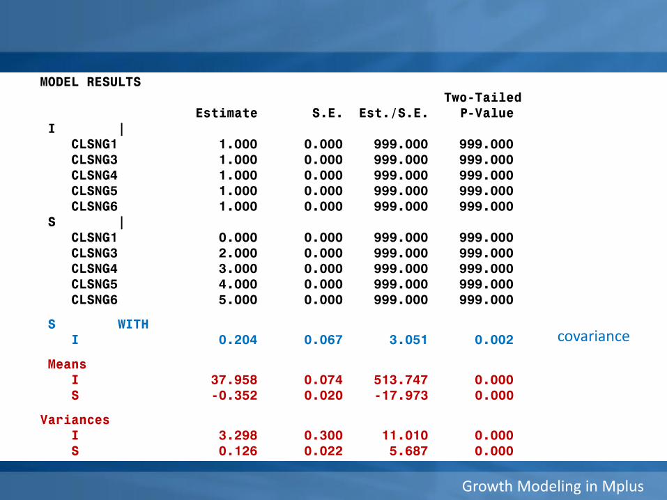
MODEL RESULTSTwo-Tailed
Estimate S.E. Est./S.E. P-ValueI |
CLSNG1 1.000 0.000 999.000 999.000CLSNG3 1.000 0.000 999.000 999.000CLSNG4 1.000 0.000 999.000 999.000CLSNG5 1.000 0.000 999.000 999.000CLSNG6 1.000 0.000 999.000 999.000
S |CLSNG1 0.000 0.000 999.000 999.000CLSNG3 2.000 0.000 999.000 999.000CLSNG4 3.000 0.000 999.000 999.000CLSNG5 4.000 0.000 999.000 999.000CLSNG6 5.000 0.000 999.000 999.000
S WITHI 0.204 0.067 3.051 0.002
MeansI 37.958 0.074 513.747 0.000S -0.352 0.020 -17.973 0.000
VariancesI 3.298 0.300 11.010 0.000S 0.126 0.022 5.687 0.000
covariance

Growth Modeling in Mplus
STDYX StandardizationTwo-Tailed
Estimate S.E. Est./S.E. P-ValueS WITHI 0.316 0.133 2.381 0.017
MeansI 20.902 0.951 21.989 0.000S -0.990 0.103 -9.587 0.000
Residual VariancesCLSNG1 0.500 0.037 13.527 0.000CLSNG3 0.416 0.019 21.638 0.000CLSNG4 0.428 0.019 22.858 0.000CLSNG5 0.348 0.019 18.578 0.000CLSNG6 0.371 0.021 18.011 0.000
R-SQUAREObserved Two-TailedVariable Estimate S.E. Est./S.E. P-ValueCLSNG1 0.500 0.037 13.527 0.000CLSNG3 0.584 0.019 30.367 0.000CLSNG4 0.572 0.019 30.610 0.000CLSNG5 0.652 0.019 34.824 0.000CLSNG6 0.629 0.021 30.539 0.000
correlation
Growth Modeling in Mplus
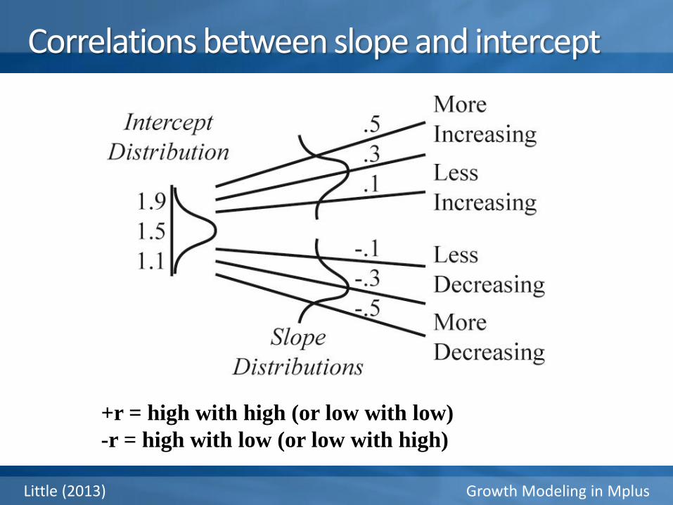
Correlations between slope and intercept
+r = high with high (or low with low)
-r = high with low (or low with high)
Little (2013)

Growth Modeling in Mplus
Fit a linear growth model using conflict G1-G6
Data set: CLSNCNFL.csv
Growth Modeling in Mplus
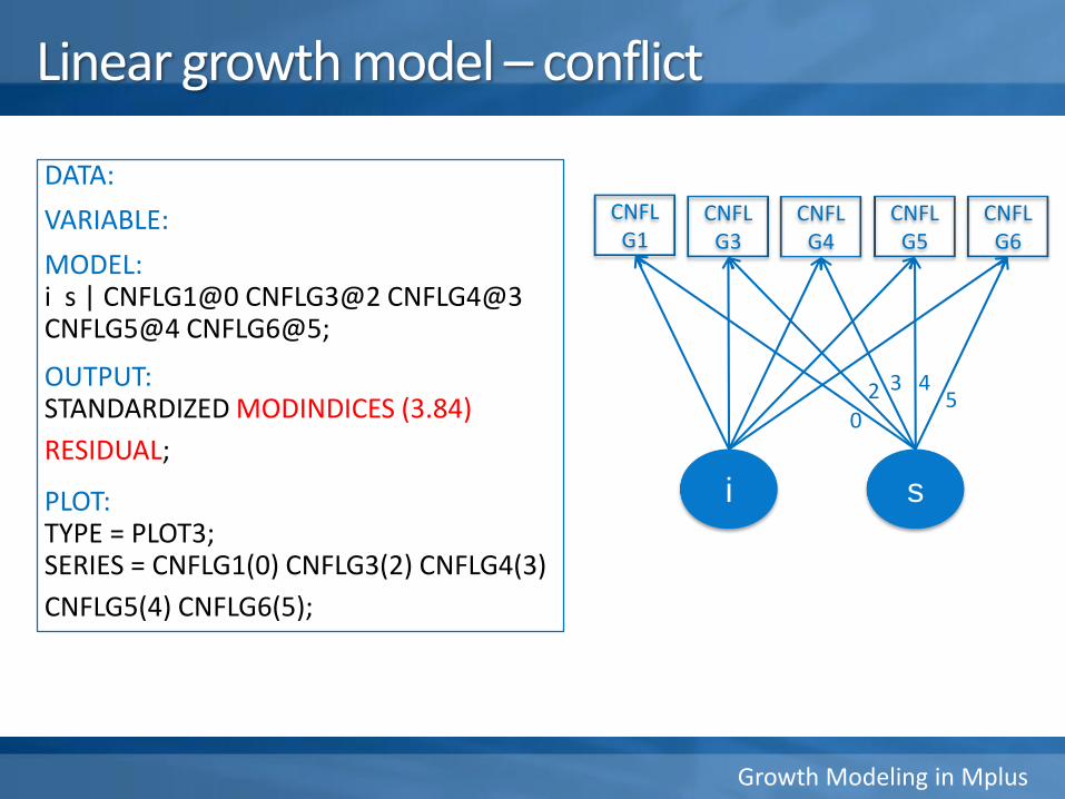
Linear growth model – conflict
DATA:
VARIABLE:
MODEL:i s | CNFLG1@0 CNFLG3@2 CNFLG4@3 CNFLG5@4 CNFLG6@5;
OUTPUT:STANDARDIZED MODINDICES (3.84)
RESIDUAL;
PLOT:TYPE = PLOT3;SERIES = CNFLG1(0) CNFLG3(2) CNFLG4(3)
CNFLG5(4) CNFLG6(5);
CNFL G1
CNFL G4
CNFL G5
CNFL G6
i s
CNFL G3
02 3 4
5
Growth Modeling in Mplus
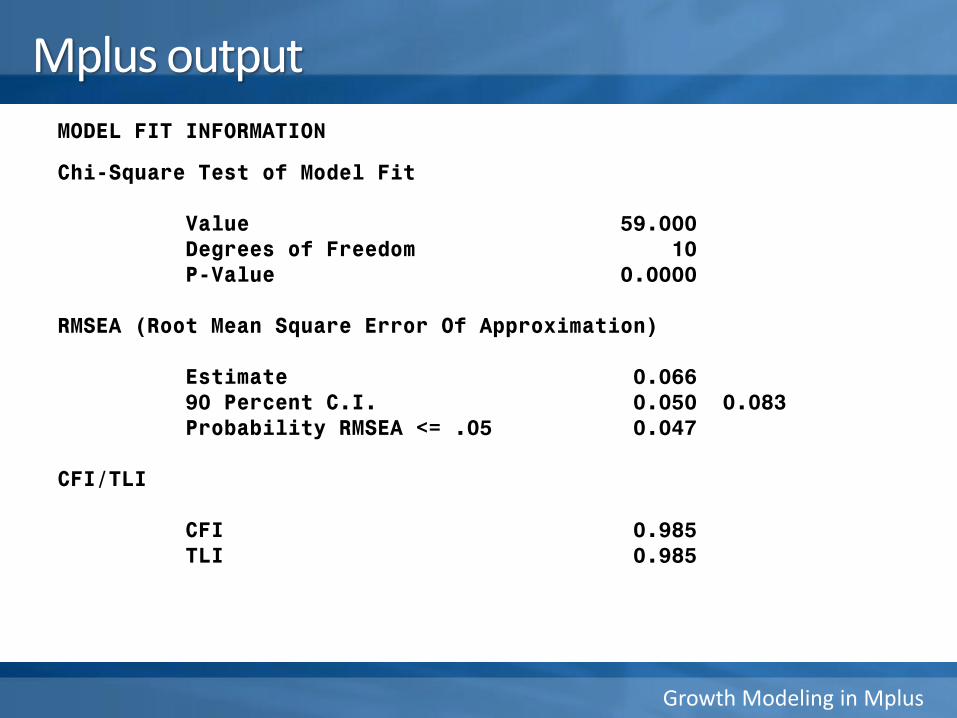
MODEL FIT INFORMATION
Chi-Square Test of Model Fit
Value 59.000Degrees of Freedom 10P-Value 0.0000
RMSEA (Root Mean Square Error Of Approximation)
Estimate 0.06690 Percent C.I. 0.050 0.083Probability RMSEA <= .05 0.047
CFI/TLI
CFI 0.985TLI 0.985
Mplus output
Growth Modeling in Mplus
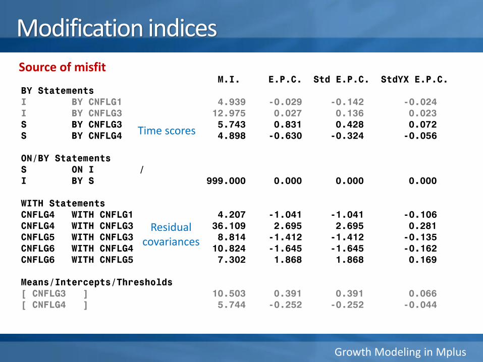
Modification indices
M.I. E.P.C. Std E.P.C. StdYX E.P.C.BY StatementsI BY CNFLG1 4.939 -0.029 -0.142 -0.024I BY CNFLG3 12.975 0.027 0.136 0.023S BY CNFLG3 5.743 0.831 0.428 0.072S BY CNFLG4 4.898 -0.630 -0.324 -0.056
ON/BY StatementsS ON I /I BY S 999.000 0.000 0.000 0.000
WITH StatementsCNFLG4 WITH CNFLG1 4.207 -1.041 -1.041 -0.106CNFLG4 WITH CNFLG3 36.109 2.695 2.695 0.281CNFLG5 WITH CNFLG3 8.814 -1.412 -1.412 -0.135CNFLG6 WITH CNFLG4 10.824 -1.645 -1.645 -0.162CNFLG6 WITH CNFLG5 7.302 1.868 1.868 0.169
Means/Intercepts/Thresholds[ CNFLG3 ] 10.503 0.391 0.391 0.066[ CNFLG4 ] 5.744 -0.252 -0.252 -0.044
Source of misfit
Time scores
Residual covariances

Growth Modeling in Mplus
Model modifications
RecommendedTime scores for slope growth factor
Residual covariances for outcomes
Not recommendedOutcome variable intercepts
Loadings for intercept growth factor

Growth Modeling in Mplus
RESIDUAL OUTPUTESTIMATED MODEL AND RESIDUALS (OBSERVED - ESTIMATED)
Model Estimated Means/Intercepts/ThresholdsCNFLG1 CNFLG3 CNFLG4 CNFLG5 CNFLG6________ ________ ________ ________ ________
1 15.271 15.840 16.125 16.409 16.694
Residuals for Means/Intercepts/ThresholdsCNFLG1 CNFLG3 CNFLG4 CNFLG5 CNFLG6________ ________ ________ ________ ________
1 -0.074 0.298 -0.184 -0.031 0.071
Standardized Residuals (z-scores) for Means/Intercepts/ThresholdsCNFLG1 CNFLG3 CNFLG4 CNFLG5 CNFLG6________ ________ ________ ________ ________
1 -1.767 3.033 -2.097 -0.381 1.055

Growth Modeling in Mplus
Sample and estimated means – conflict

Growth Modeling in Mplus
Unconditional growth model – Nonlinear growth
Growth Modeling in Mplus
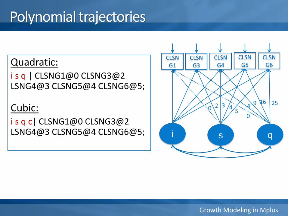
Polynomial trajectories
CLSN G3
CLSN G4
CLSN G5
CLSN G6
i s
20 35
CLSN G1
4
q
0
4 9 16 25
Quadratic:i s q | CLSNG1@0 CLSNG3@2 LSNG4@3 CLSNG5@4 CLSNG6@5;
Cubic:i s q c| CLSNG1@0 CLSNG3@2 LSNG4@3 CLSNG5@4 CLSNG6@5;
Growth Modeling in Mplus
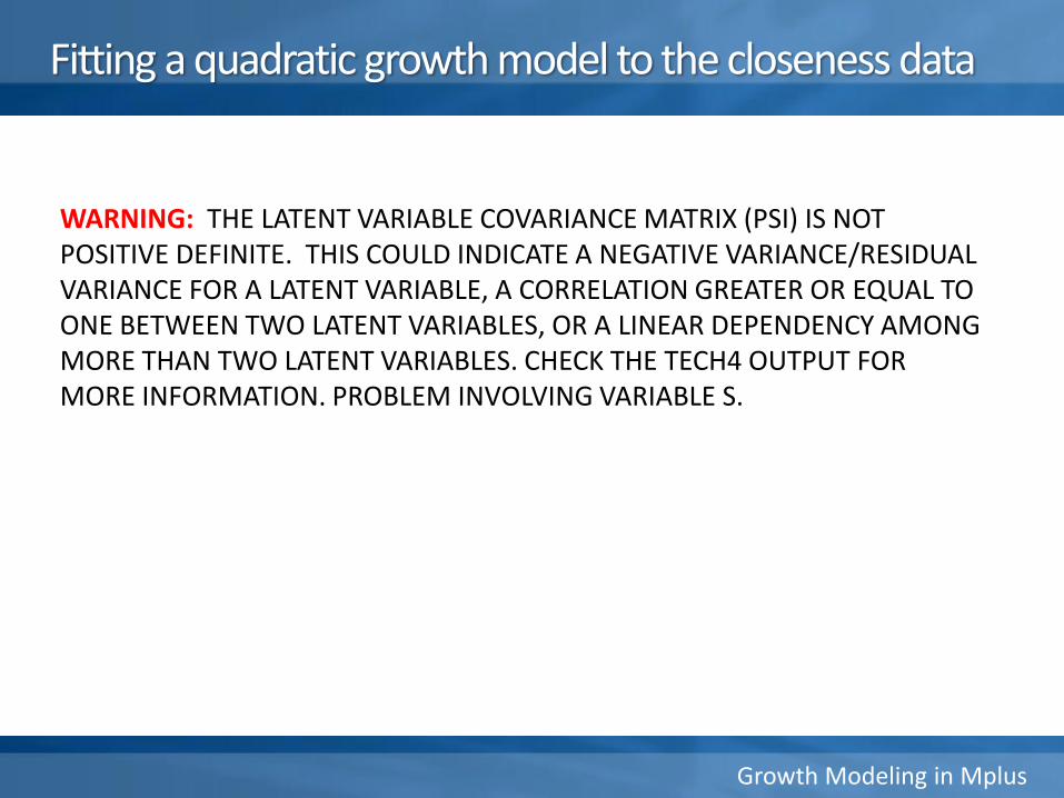
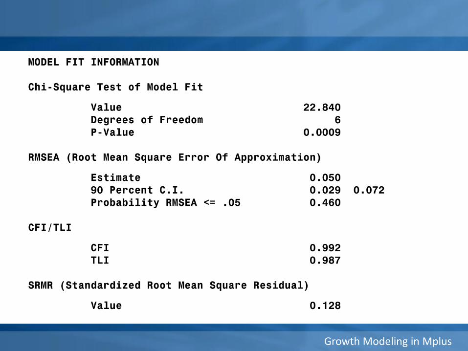
Fitting a quadratic growth model to the closeness data
WARNING: THE LATENT VARIABLE COVARIANCE MATRIX (PSI) IS NOT POSITIVE DEFINITE. THIS COULD INDICATE A NEGATIVE VARIANCE/RESIDUAL VARIANCE FOR A LATENT VARIABLE, A CORRELATION GREATER OR EQUAL TO ONE BETWEEN TWO LATENT VARIABLES, OR A LINEAR DEPENDENCY AMONG MORE THAN TWO LATENT VARIABLES. CHECK THE TECH4 OUTPUT FOR MORE INFORMATION. PROBLEM INVOLVING VARIABLE S.
Growth Modeling in Mplus
MODEL FIT INFORMATION
Chi-Square Test of Model Fit
Value 22.840Degrees of Freedom 6P-Value 0.0009
RMSEA (Root Mean Square Error Of Approximation)
Estimate 0.05090 Percent C.I. 0.029 0.072Probability RMSEA <= .05 0.460
CFI/TLI
CFI 0.992TLI 0.987
SRMR (Standardized Root Mean Square Residual)
Value 0.128
Growth Modeling in Mplus
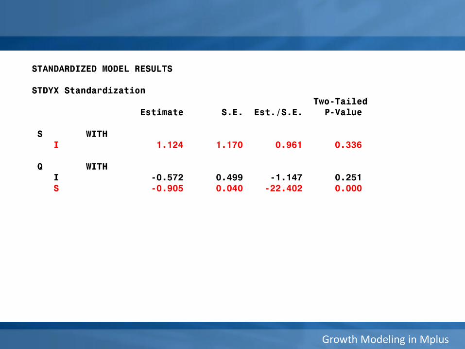
STANDARDIZED MODEL RESULTS
STDYX StandardizationTwo-Tailed
Estimate S.E. Est./S.E. P-Value
S WITHI 1.124 1.170 0.961 0.336
Q WITHI -0.572 0.499 -1.147 0.251S -0.905 0.040 -22.402 0.000

Growth Modeling in Mplus
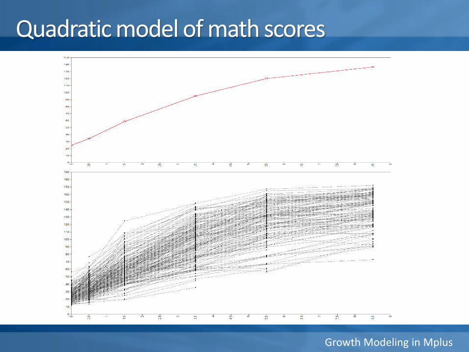
Fit a quadratic model to math scores from kindergarten to grade 8 using the “MathReading.csv” data set
MODEL:i s q| mathK@0 mathG1@1 mathG3@3 mathG5@5 mathG8@8;
Growth Modeling in Mplus
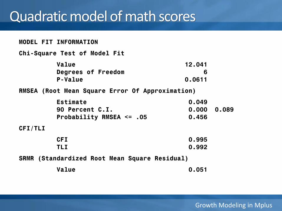
Quadratic model of math scores
Growth Modeling in Mplus
MODEL FIT INFORMATION
Chi-Square Test of Model Fit
Value 12.041Degrees of Freedom 6P-Value 0.0611
RMSEA (Root Mean Square Error Of Approximation)
Estimate 0.04990 Percent C.I. 0.000 0.089Probability RMSEA <= .05 0.456
CFI/TLI
CFI 0.995TLI 0.992
SRMR (Standardized Root Mean Square Residual)
Value 0.051
Quadratic model of math scores

Growth Modeling in Mplus
MODEL RESULTSTwo-Tailed
Estimate S.E. Est./S.E. P-ValueS WITH
I 33.424 5.969 5.600 0.000
Q WITHI -3.474 0.611 -5.689 0.000S -4.661 0.618 -7.547 0.000
MeansI 34.590 0.552 62.656 0.000S 24.704 0.446 55.445 0.000Q -1.494 0.047 -31.588 0.000
VariancesI 114.294 10.799 10.583 0.000S 50.657 5.715 8.863 0.000Q 0.462 0.078 5.890 0.000
R-SQUAREMATHK 0.912 0.056 16.424 0.000MATHG1 0.707 0.025 28.472 0.000MATHG3 0.882 0.021 41.751 0.000MATHG5 0.883 0.019 45.430 0.000MATHG8 0.982 0.081 12.098 0.000
Growth Modeling in Mplus
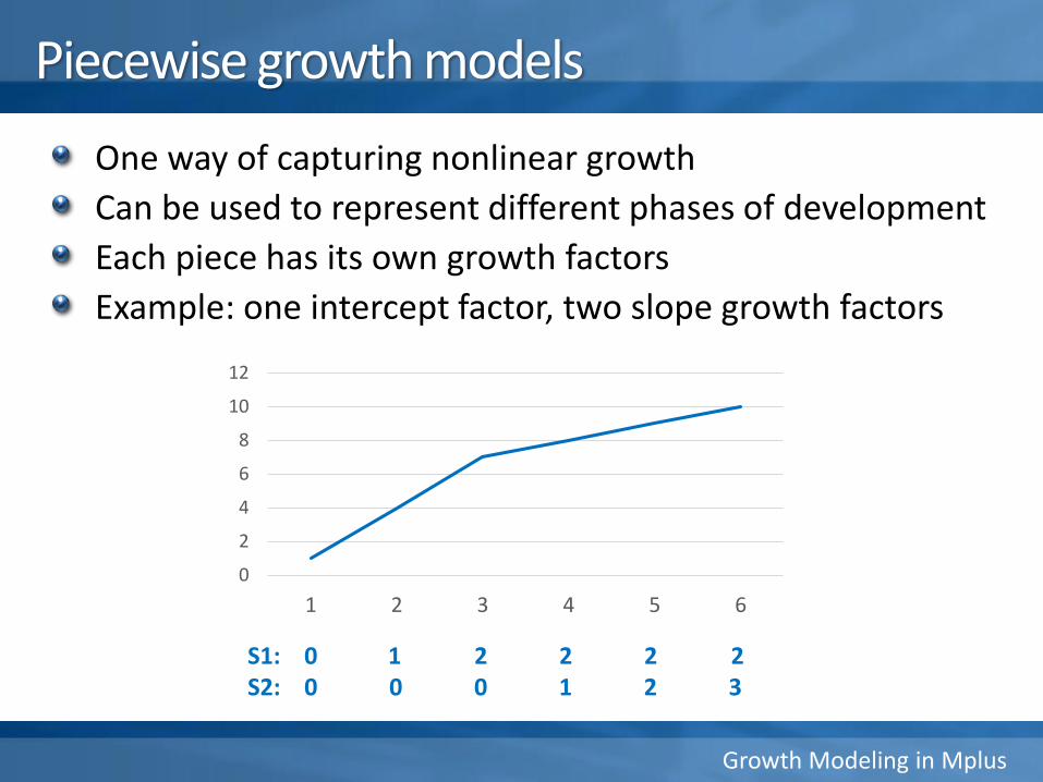
Piecewise growth models
One way of capturing nonlinear growth
Can be used to represent different phases of development
Each piece has its own growth factors
Example: one intercept factor, two slope growth factors
S1: 0 1 2 2 2 2S2: 0 0 0 1 2 3
0
2
4
6
8
10
12
1 2 3 4 5 6

Growth Modeling in Mplus
Fitting the closeness data
CLSN G3
CLSN G4
CLSN G5
CLSN G6
i s1
20 33
CLSN G1
3
s2
0
0 0 1 2
MODEL:i s1 | CLSNG1@0 CLSNG3@2 LSNG4@3 CLSNG5@3 CLSNG6@3;
i s2 | CLSNG1@0 CLSNG3@0 LSNG4@0 CLSNG5@1 CLSNG6@2;
Growth Modeling in Mplus
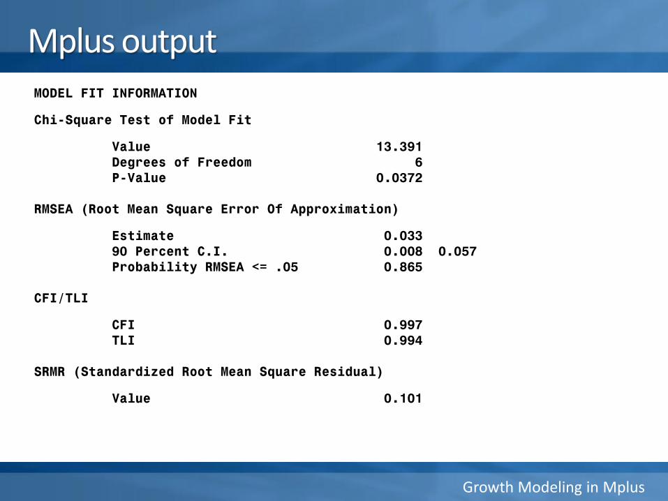
Mplus outputMODEL FIT INFORMATION
Chi-Square Test of Model Fit
Value 13.391Degrees of Freedom 6P-Value 0.0372
RMSEA (Root Mean Square Error Of Approximation)
Estimate 0.03390 Percent C.I. 0.008 0.057Probability RMSEA <= .05 0.865
CFI/TLI
CFI 0.997TLI 0.994
SRMR (Standardized Root Mean Square Residual)
Value 0.101
Growth Modeling in Mplus
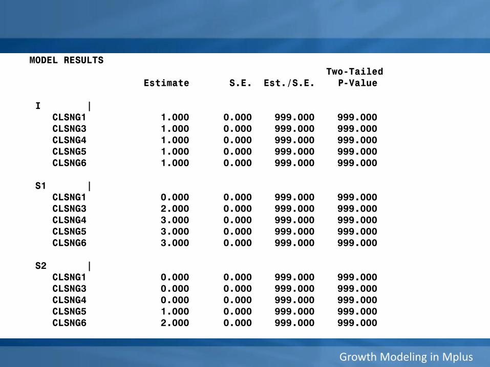
MODEL RESULTSTwo-Tailed
Estimate S.E. Est./S.E. P-Value
I |CLSNG1 1.000 0.000 999.000 999.000CLSNG3 1.000 0.000 999.000 999.000CLSNG4 1.000 0.000 999.000 999.000CLSNG5 1.000 0.000 999.000 999.000CLSNG6 1.000 0.000 999.000 999.000
S1 |CLSNG1 0.000 0.000 999.000 999.000CLSNG3 2.000 0.000 999.000 999.000CLSNG4 3.000 0.000 999.000 999.000CLSNG5 3.000 0.000 999.000 999.000CLSNG6 3.000 0.000 999.000 999.000
S2 |CLSNG1 0.000 0.000 999.000 999.000CLSNG3 0.000 0.000 999.000 999.000CLSNG4 0.000 0.000 999.000 999.000CLSNG5 1.000 0.000 999.000 999.000CLSNG6 2.000 0.000 999.000 999.000
Growth Modeling in Mplus
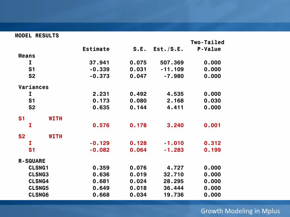
MODEL RESULTSTwo-Tailed
Estimate S.E. Est./S.E. P-ValueMeans
I 37.941 0.075 507.369 0.000S1 -0.339 0.031 -11.109 0.000S2 -0.373 0.047 -7.980 0.000
VariancesI 2.231 0.492 4.535 0.000S1 0.173 0.080 2.168 0.030S2 0.635 0.144 4.411 0.000
S1 WITHI 0.576 0.178 3.240 0.001
S2 WITHI -0.129 0.128 -1.010 0.312S1 -0.082 0.064 -1.283 0.199
R-SQUARECLSNG1 0.359 0.076 4.727 0.000CLSNG3 0.636 0.019 32.710 0.000CLSNG4 0.681 0.024 28.295 0.000CLSNG5 0.649 0.018 36.444 0.000CLSNG6 0.668 0.034 19.736 0.000
Growth Modeling in Mplus
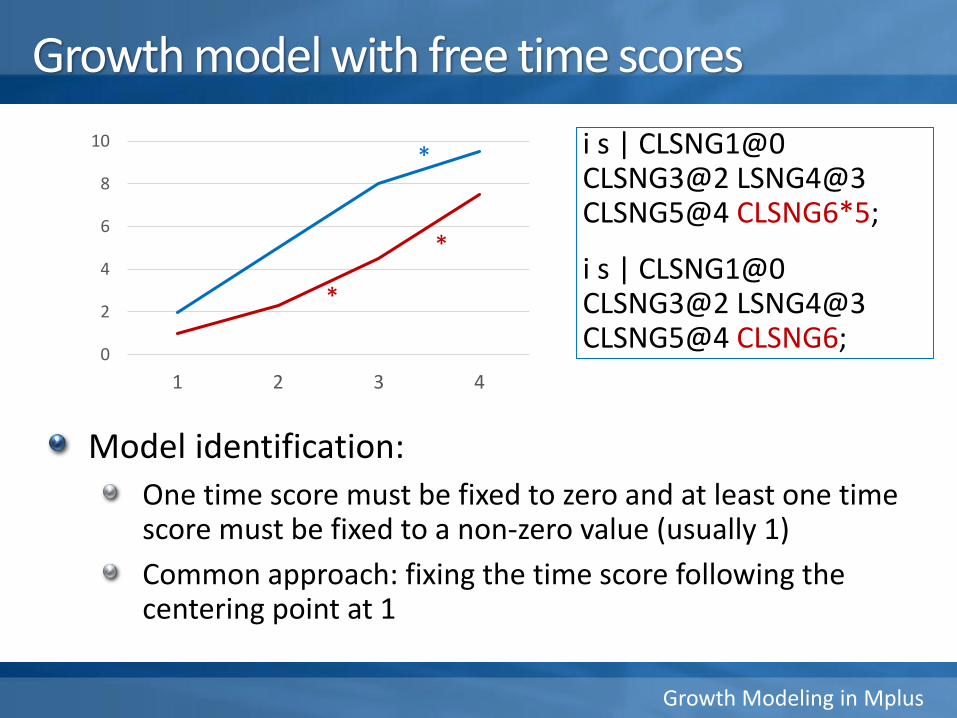
Growth model with free time scores
Model identification:
One time score must be fixed to zero and at least one time score must be fixed to a non-zero value (usually 1)
Common approach: fixing the time score following the centering point at 1
0
2
4
6
8
10
1 2 3 4
*
*
*
i s | CLSNG1@0 CLSNG3@2 LSNG4@3 CLSNG5@4 CLSNG6*5;
i s | CLSNG1@0 CLSNG3@2 LSNG4@3 CLSNG5@4 CLSNG6;
Growth Modeling in Mplus
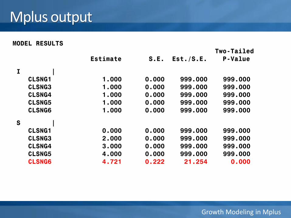
MODEL RESULTSTwo-Tailed
Estimate S.E. Est./S.E. P-Value
I |CLSNG1 1.000 0.000 999.000 999.000CLSNG3 1.000 0.000 999.000 999.000CLSNG4 1.000 0.000 999.000 999.000CLSNG5 1.000 0.000 999.000 999.000CLSNG6 1.000 0.000 999.000 999.000
S |CLSNG1 0.000 0.000 999.000 999.000CLSNG3 2.000 0.000 999.000 999.000CLSNG4 3.000 0.000 999.000 999.000CLSNG5 4.000 0.000 999.000 999.000CLSNG6 4.721 0.222 21.254 0.000
Mplus output

Growth Modeling in Mplus
Conditional growth models
Growth Modeling in Mplus
Conditional growth models
Adding covariates to the growth model
Types of covariatesTime-invariant covariates: vary across individuals not time
Time-varying covariates: vary across time and individual
Growth Modeling in Mplus
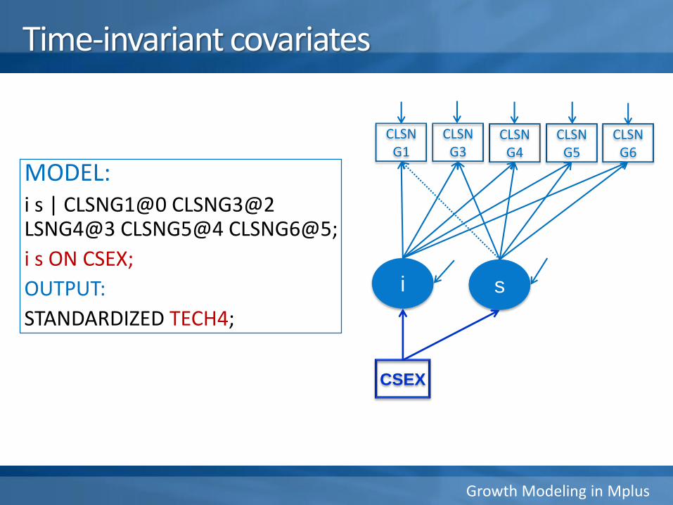
Time-invariant covariates
CLSN G1
CLSN G3
CLSN G4
CLSN G5
i s
MODEL:i s | CLSNG1@0 CLSNG3@2 LSNG4@3 CLSNG5@4 CLSNG6@5;
i s ON CSEX;
OUTPUT:
STANDARDIZED TECH4;
CLSN G6
CSEX

Growth Modeling in Mplus
Gender as time-invariant covariate – output
MODEL FIT INFORMATION
Chi-Square Test of Model Fit
Value 65.865
Degrees of Freedom 13
P-Value 0.0000
RMSEA (Root Mean Square Error Of Approximation)
Estimate 0.060
90 Percent C.I. 0.046 0.075
Probability RMSEA <= .05 0.113
CFI/TLI
CFI 0.976
TLI 0.972
Growth Modeling in Mplus
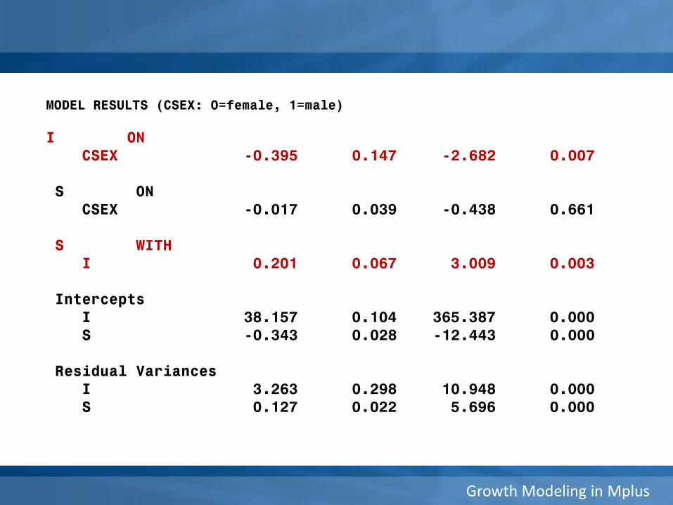
MODEL RESULTS (CSEX: 0=female, 1=male)
I ONCSEX -0.395 0.147 -2.682 0.007
S ONCSEX -0.017 0.039 -0.438 0.661
S WITHI 0.201 0.067 3.009 0.003
InterceptsI 38.157 0.104 365.387 0.000S -0.343 0.028 -12.443 0.000
Residual VariancesI 3.263 0.298 10.948 0.000S 0.127 0.022 5.696 0.000
Growth Modeling in Mplus
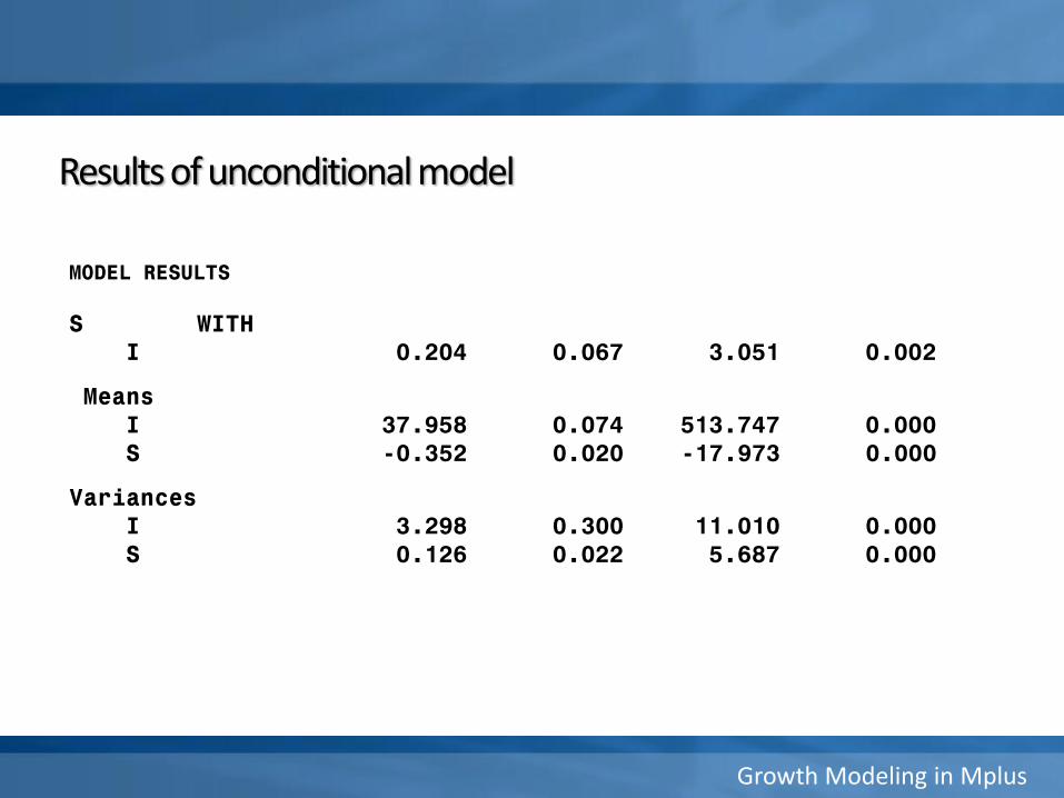
MODEL RESULTS
S WITHI 0.204 0.067 3.051 0.002
MeansI 37.958 0.074 513.747 0.000S -0.352 0.020 -17.973 0.000
VariancesI 3.298 0.300 11.010 0.000S 0.126 0.022 5.687 0.000
Results of unconditional model
Growth Modeling in Mplus
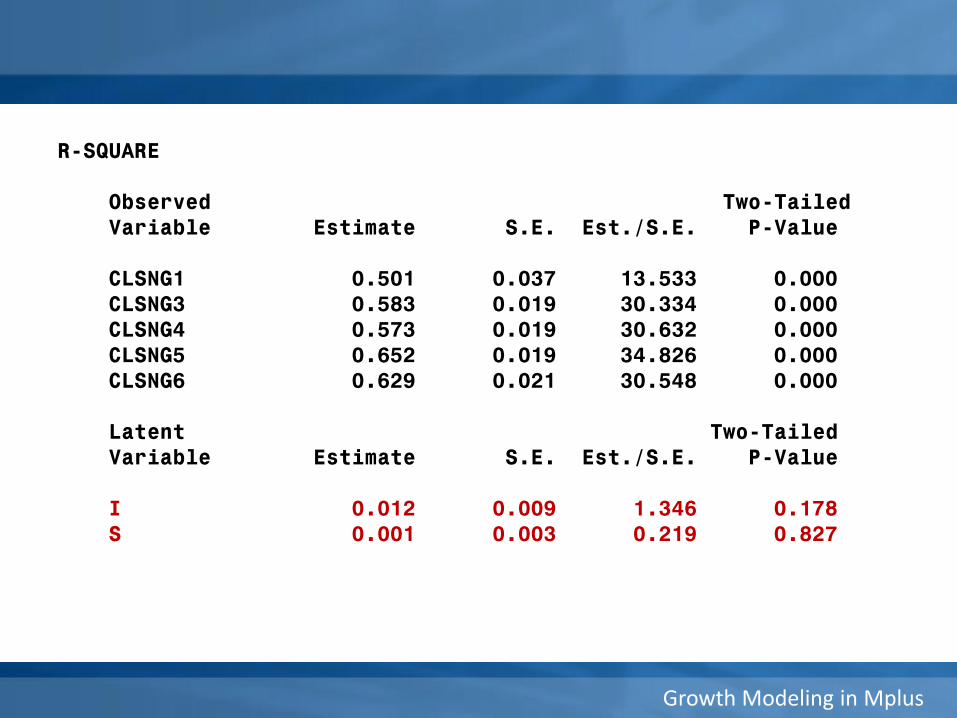
R-SQUARE
Observed Two-TailedVariable Estimate S.E. Est./S.E. P-Value
CLSNG1 0.501 0.037 13.533 0.000CLSNG3 0.583 0.019 30.334 0.000CLSNG4 0.573 0.019 30.632 0.000CLSNG5 0.652 0.019 34.826 0.000CLSNG6 0.629 0.021 30.548 0.000
Latent Two-TailedVariable Estimate S.E. Est./S.E. P-Value
I 0.012 0.009 1.346 0.178S 0.001 0.003 0.219 0.827
Growth Modeling in Mplus
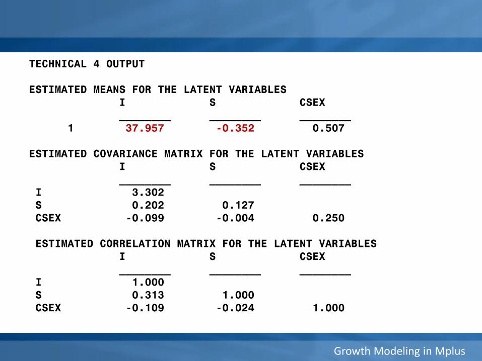
TECHNICAL 4 OUTPUT
ESTIMATED MEANS FOR THE LATENT VARIABLESI S CSEX________ ________ ________
1 37.957 -0.352 0.507
ESTIMATED COVARIANCE MATRIX FOR THE LATENT VARIABLESI S CSEX________ ________ ________
I 3.302S 0.202 0.127CSEX -0.099 -0.004 0.250
ESTIMATED CORRELATION MATRIX FOR THE LATENT VARIABLESI S CSEX________ ________ ________
I 1.000S 0.313 1.000CSEX -0.109 -0.024 1.000
Growth Modeling in Mplus
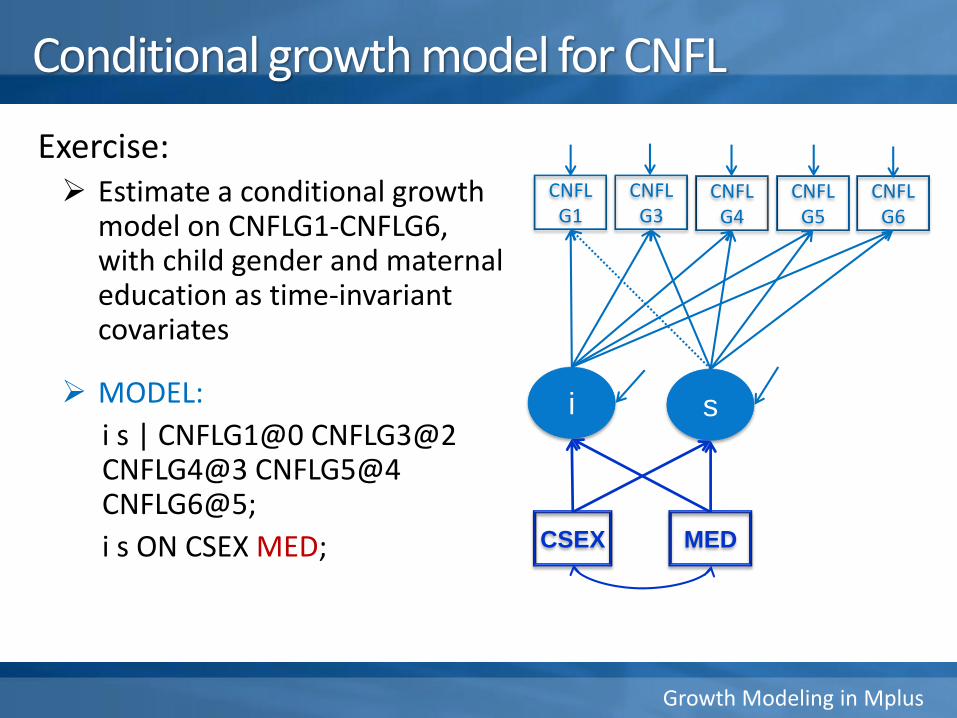
Conditional growth model for CNFL
CNFL G1
CNFL G3
CNFL G4
CNFL G5
i s
Exercise: Estimate a conditional growth
model on CNFLG1-CNFLG6, with child gender and maternal education as time-invariant covariates
MODEL:
i s | CNFLG1@0 CNFLG3@2 CNFLG4@3 CNFLG5@4 CNFLG6@5;
i s ON CSEX MED;
CNFL G6
CSEX MED

Growth Modeling in Mplus
MODEL FIT INFORMATION
Chi-Square Test of Model Fit
Value 64.257Degrees of Freedom 16P-Value 0.0000
RMSEA (Root Mean Square Error Of Approximation)
Estimate 0.05290 Percent C.I. 0.039 0.065Probability RMSEA <= .05 0.390
CFI/TLI
CFI 0.985TLI 0.982
SRMR (Standardized Root Mean Square Residual)
Value 0.030
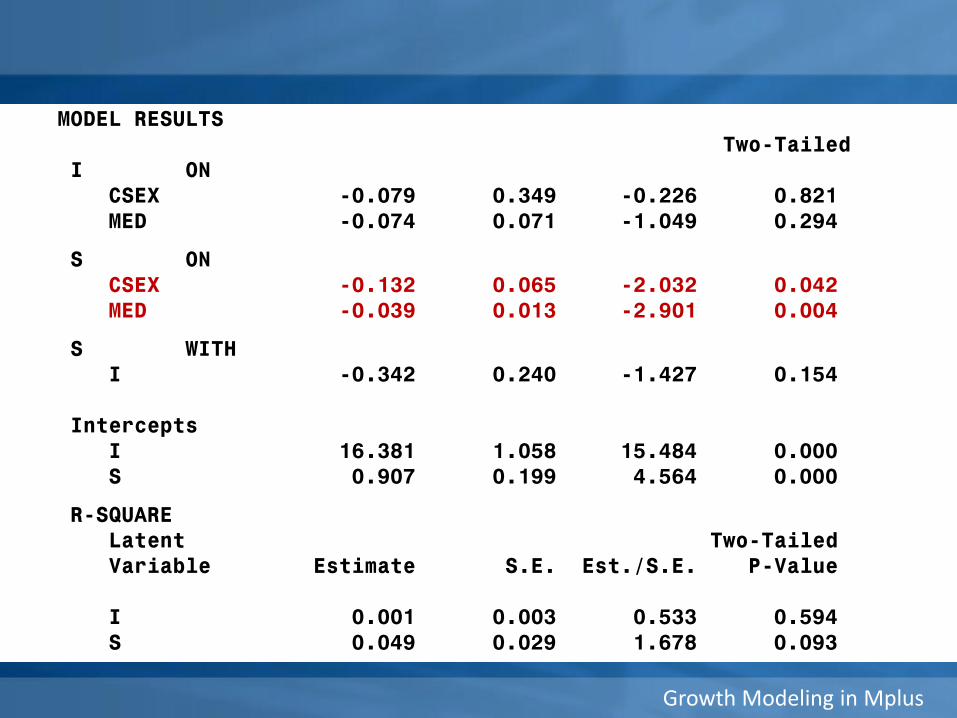
Mplus output
Growth Modeling in Mplus
MODEL RESULTSTwo-Tailed
I ONCSEX -0.079 0.349 -0.226 0.821MED -0.074 0.071 -1.049 0.294
S ONCSEX -0.132 0.065 -2.032 0.042MED -0.039 0.013 -2.901 0.004
S WITHI -0.342 0.240 -1.427 0.154
InterceptsI 16.381 1.058 15.484 0.000S 0.907 0.199 4.564 0.000
R-SQUARELatent Two-TailedVariable Estimate S.E. Est./S.E. P-Value
I 0.001 0.003 0.533 0.594S 0.049 0.029 1.678 0.093
Growth Modeling in Mplus
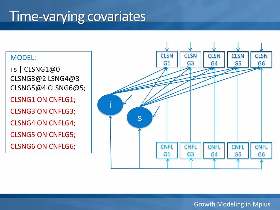
Time-varying covariates
CLSN G1
CLSN G3
CLSN G4
CLSN G5
i
s
CLSN G6
CNFL G1
CNFL G3
CNFL G4
CNFL G5
CNFL G6
MODEL:
i s | CLSNG1@0 CLSNG3@2 LSNG4@3 CLSNG5@4 CLSNG6@5;
CLSNG1 ON CNFLG1;
CLSNG3 ON CNFLG3;
CLSNG4 ON CNFLG4;
CLSNG5 ON CNFLG5;
CLSNG6 ON CNFLG6;
Growth Modeling in Mplus
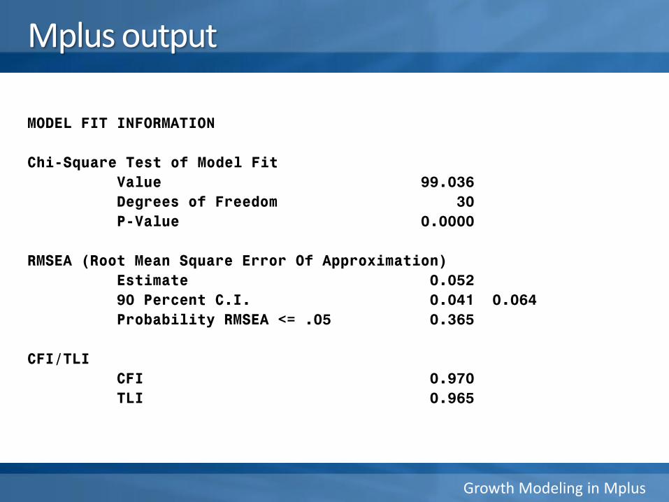
Mplus output
MODEL FIT INFORMATION
Chi-Square Test of Model Fit
Value 99.036
Degrees of Freedom 30
P-Value 0.0000
RMSEA (Root Mean Square Error Of Approximation)
Estimate 0.052
90 Percent C.I. 0.041 0.064
Probability RMSEA <= .05 0.365
CFI/TLI
CFI 0.970
TLI 0.965

Growth Modeling in Mplus
MODEL RESULTS
Two-Tailed
Estimate S.E. Est./S.E. P-Value
CLSNG1 ON
CNFLG1 -0.123 0.011 -11.207 0.000
CLSNG3 ON
CNFLG3 -0.140 0.008 -16.505 0.000
CLSNG4 ON
CNFLG4 -0.150 0.009 -16.035 0.000
CLSNG5 ON
CNFLG5 -0.165 0.010 -15.856 0.000
CLSNG6 ON
CNFLG6 -0.181 0.012 -14.855 0.000
Growth Modeling in Mplus
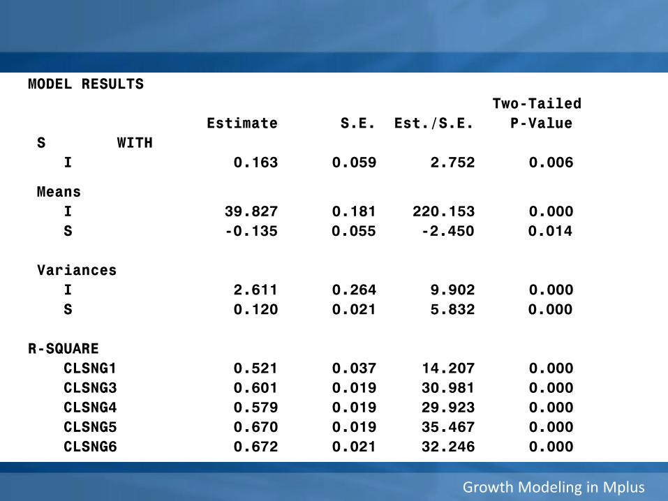
MODEL RESULTS
Two-Tailed
Estimate S.E. Est./S.E. P-Value
S WITH
I 0.163 0.059 2.752 0.006
Means
I 39.827 0.181 220.153 0.000
S -0.135 0.055 -2.450 0.014
Variances
I 2.611 0.264 9.902 0.000
S 0.120 0.021 5.832 0.000
R-SQUARE
CLSNG1 0.521 0.037 14.207 0.000
CLSNG3 0.601 0.019 30.981 0.000
CLSNG4 0.579 0.019 29.923 0.000
CLSNG5 0.670 0.019 35.467 0.000
CLSNG6 0.672 0.021 32.246 0.000

Growth Modeling in Mplus
Time-varying and time-invariant covariates
CLSN G1
CLSN G3
CLSN G4
CLSN G5
i
s
CLSN G6
CNFL G1
CNFL G3
CNFL G4
CNFL G5
CNFL G6
CSEX MED
MODEL:
i s | CLSNG1@0 CLSNG3@2 LSNG4@3 CLSNG5@4 CLSNG6@5;
i s ON CSEX MED;
CLSNG1 ON CNFLG1;
CLSNG3 ON CNFLG3;
CLSNG4 ON CNFLG4;
CLSNG5 ON CNFLG5;
CLSNG6 ON CNFLG6;
Growth Modeling in Mplus
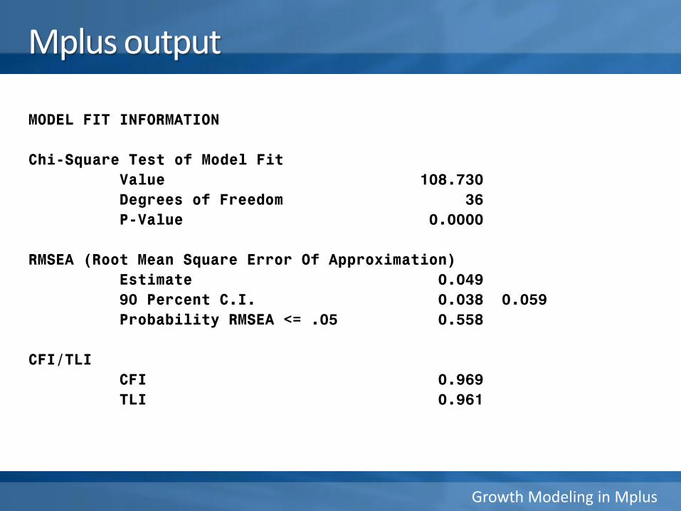
Mplus output
MODEL FIT INFORMATION
Chi-Square Test of Model Fit
Value 108.730
Degrees of Freedom 36
P-Value 0.0000
RMSEA (Root Mean Square Error Of Approximation)
Estimate 0.049
90 Percent C.I. 0.038 0.059
Probability RMSEA <= .05 0.558
CFI/TLI
CFI 0.969
TLI 0.961
Growth Modeling in Mplus
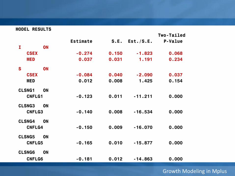
MODEL RESULTS
Two-Tailed
Estimate S.E. Est./S.E. P-Value
I ON
CSEX -0.274 0.150 -1.823 0.068
MED 0.037 0.031 1.191 0.234
S ON
CSEX -0.084 0.040 -2.090 0.037
MED 0.012 0.008 1.425 0.154
CLSNG1 ON
CNFLG1 -0.123 0.011 -11.211 0.000
CLSNG3 ON
CNFLG3 -0.140 0.008 -16.534 0.000
CLSNG4 ON
CNFLG4 -0.150 0.009 -16.070 0.000
CLSNG5 ON
CNFLG5 -0.165 0.010 -15.877 0.000
CLSNG6 ON
CNFLG6 -0.181 0.012 -14.863 0.000
Growth Modeling in Mplus
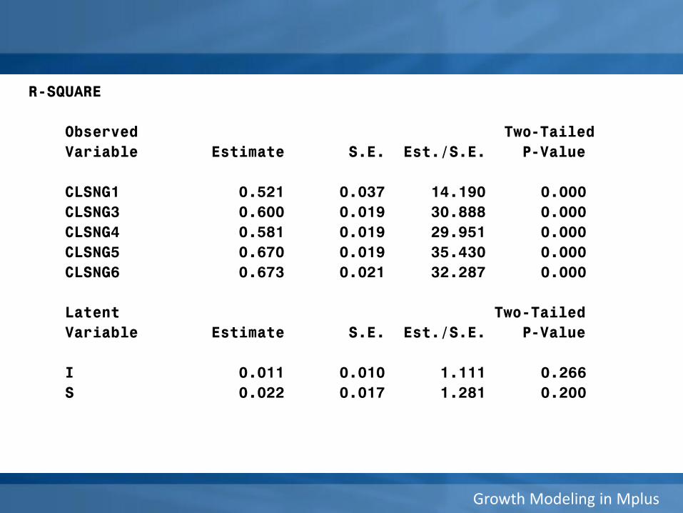
R-SQUARE
Observed Two-Tailed
Variable Estimate S.E. Est./S.E. P-Value
CLSNG1 0.521 0.037 14.190 0.000
CLSNG3 0.600 0.019 30.888 0.000
CLSNG4 0.581 0.019 29.951 0.000
CLSNG5 0.670 0.019 35.430 0.000
CLSNG6 0.673 0.021 32.287 0.000
Latent Two-Tailed
Variable Estimate S.E. Est./S.E. P-Value
I 0.011 0.010 1.111 0.266
S 0.022 0.017 1.281 0.200
Growth Modeling in Mplus
Run a linear growth model on CNFLG1-CNFLG6, with CLSNG1-CLSNG6 as time-varying covariates and CSEX and MED as time-invariant covariates.
Growth Modeling in Mplus
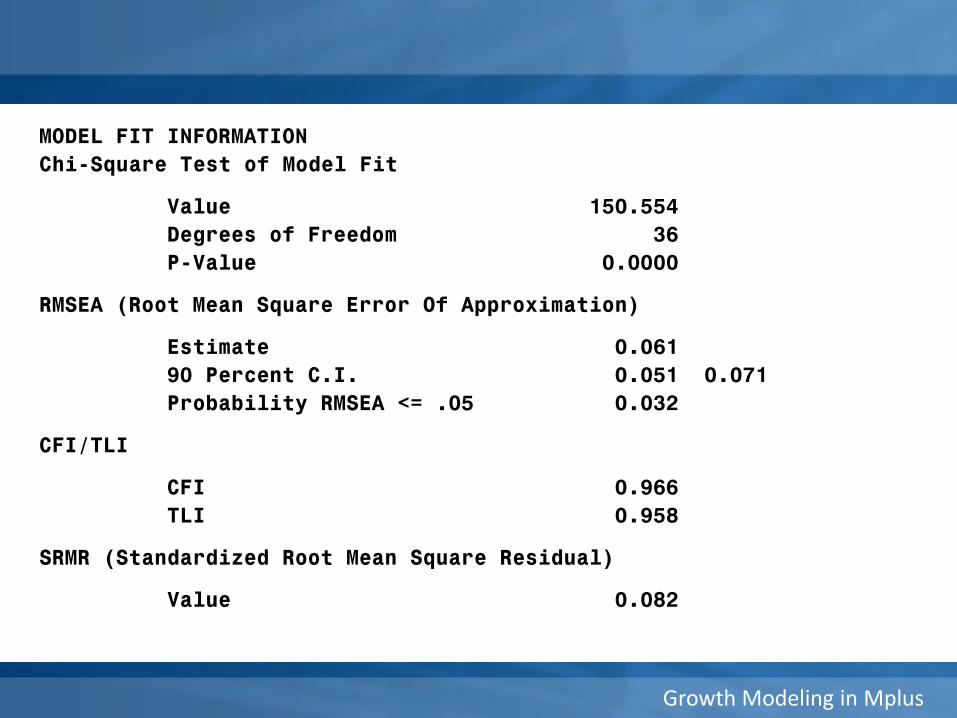
MODEL FIT INFORMATION
Chi-Square Test of Model Fit
Value 150.554
Degrees of Freedom 36
P-Value 0.0000
RMSEA (Root Mean Square Error Of Approximation)
Estimate 0.061
90 Percent C.I. 0.051 0.071
Probability RMSEA <= .05 0.032
CFI/TLI
CFI 0.966
TLI 0.958
SRMR (Standardized Root Mean Square Residual)
Value 0.082
Growth Modeling in Mplus
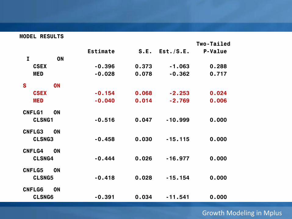
MODEL RESULTS
Two-Tailed
Estimate S.E. Est./S.E. P-Value
I ON
CSEX -0.396 0.373 -1.063 0.288
MED -0.028 0.078 -0.362 0.717
S ON
CSEX -0.154 0.068 -2.253 0.024
MED -0.040 0.014 -2.769 0.006
CNFLG1 ON
CLSNG1 -0.516 0.047 -10.999 0.000
CNFLG3 ON
CLSNG3 -0.458 0.030 -15.115 0.000
CNFLG4 ON
CLSNG4 -0.444 0.026 -16.977 0.000
CNFLG5 ON
CLSNG5 -0.418 0.028 -15.154 0.000
CNFLG6 ON
CLSNG6 -0.391 0.034 -11.541 0.000
Growth Modeling in Mplus
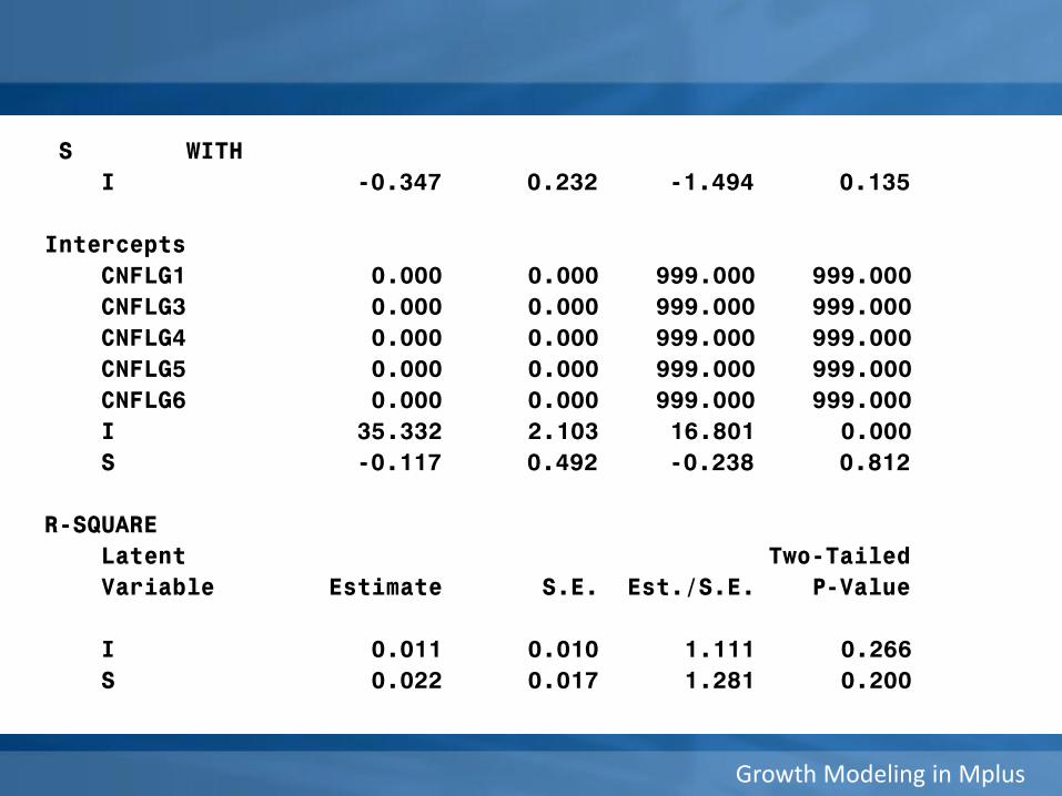
S WITH
I -0.347 0.232 -1.494 0.135
Intercepts
CNFLG1 0.000 0.000 999.000 999.000
CNFLG3 0.000 0.000 999.000 999.000
CNFLG4 0.000 0.000 999.000 999.000
CNFLG5 0.000 0.000 999.000 999.000
CNFLG6 0.000 0.000 999.000 999.000
I 35.332 2.103 16.801 0.000
S -0.117 0.492 -0.238 0.812
R-SQUARE
Latent Two-Tailed
Variable Estimate S.E. Est./S.E. P-Value
I 0.011 0.010 1.111 0.266
S 0.022 0.017 1.281 0.200
Growth Modeling in Mplus
Multivariate growth models
Growth Modeling in Mplus
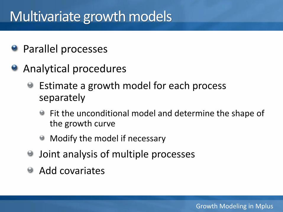
Multivariate growth models
Parallel processes
Analytical procedures
Estimate a growth model for each process separately
Fit the unconditional model and determine the shape of the growth curve
Modify the model if necessary
Joint analysis of multiple processes
Add covariates
Growth Modeling in Mplus
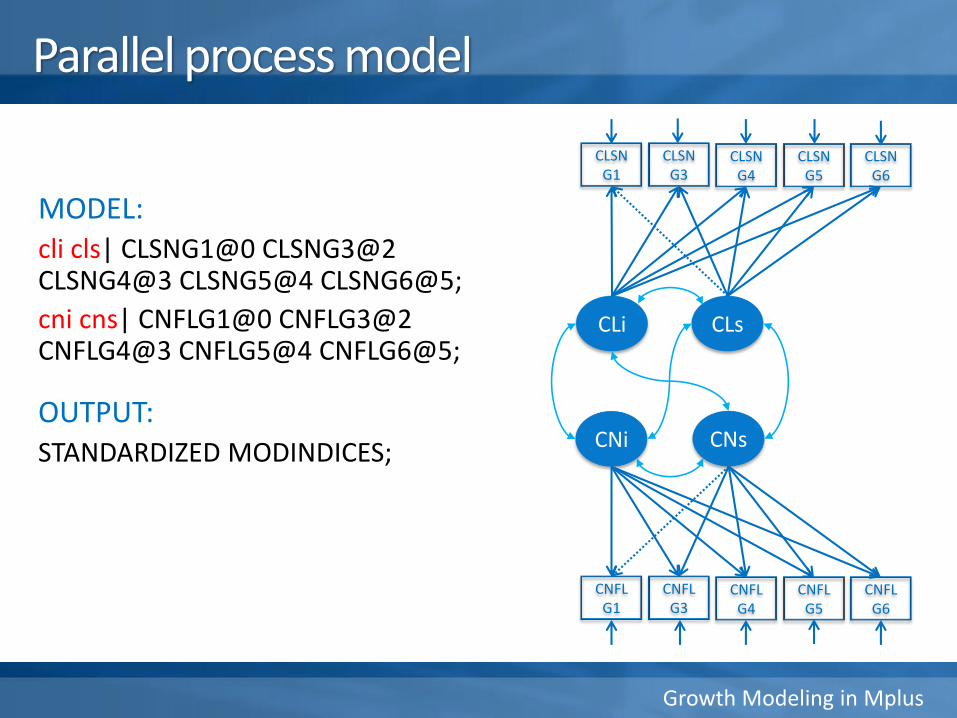
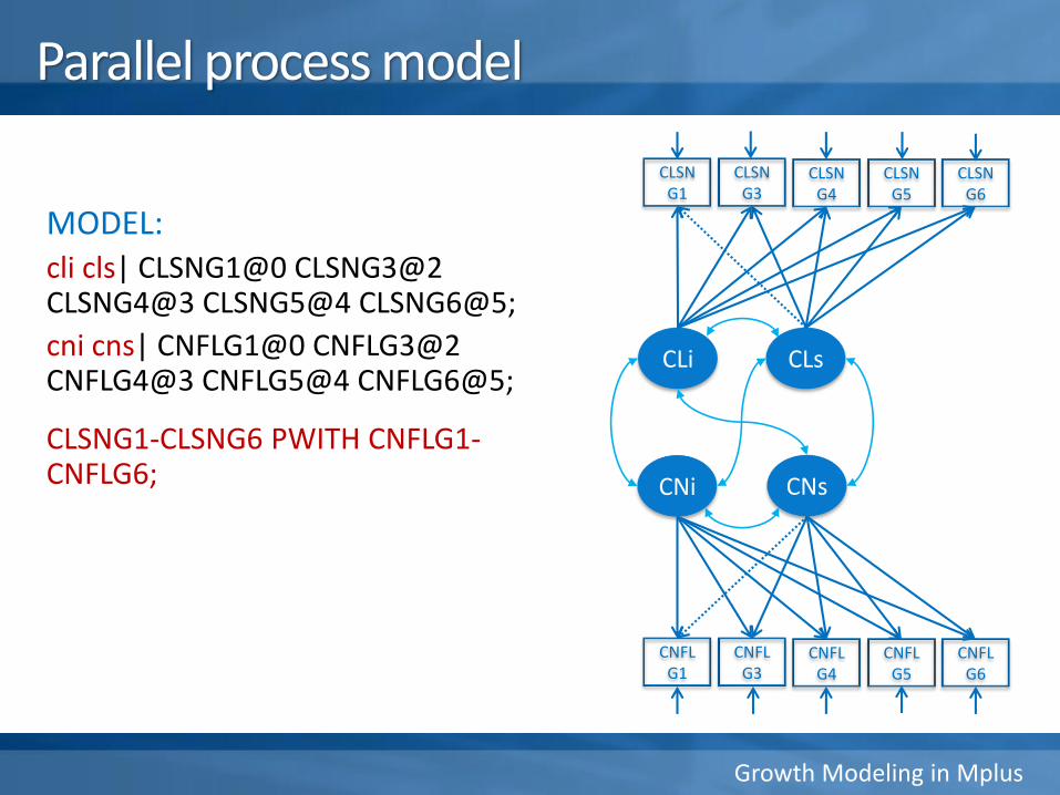
Parallel process model
CLSN G1
CLSN G3
CLSN G4
CLSN G5
CLi CLs
CLSN G6
MODEL:cli cls| CLSNG1@0 CLSNG3@2 CLSNG4@3 CLSNG5@4 CLSNG6@5;
cni cns| CNFLG1@0 CNFLG3@2 CNFLG4@3 CNFLG5@4 CNFLG6@5;
OUTPUT:STANDARDIZED MODINDICES;
CNFL G1
CNFL G3
CNFL G4
CNFL G5
CNi CNs
CNFL G6
Growth Modeling in Mplus
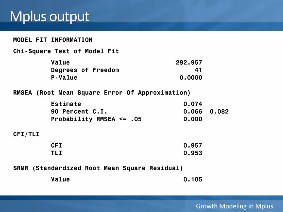
MODEL FIT INFORMATION
Chi-Square Test of Model Fit
Value 292.957Degrees of Freedom 41P-Value 0.0000
RMSEA (Root Mean Square Error Of Approximation)
Estimate 0.07490 Percent C.I. 0.066 0.082Probability RMSEA <= .05 0.000
CFI/TLI
CFI 0.957TLI 0.953
SRMR (Standardized Root Mean Square Residual)
Value 0.105
Mplus output

Growth Modeling in Mplus
CLS WITHCLI 0.185 0.067 2.760 0.006
CNI WITHCLI -4.879 0.461 -10.593 0.000CLS -0.140 0.115 -1.225 0.221
CNS WITHCLI 0.365 0.082 4.480 0.000CLS -0.148 0.021 -6.908 0.000CNI -0.366 0.241 -1.522 0.128
MeansCLI 37.956 0.074 513.261 0.000CLS -0.351 0.020 -17.939 0.000CNI 15.279 0.175 87.458 0.000CNS 0.283 0.033 8.647 0.000
VariancesCLI 3.373 0.301 11.216 0.000CLS 0.132 0.022 5.928 0.000CNI 24.696 1.505 16.404 0.000CNS 0.280 0.062 4.507 0.000

Growth Modeling in Mplus
MODEL MODIFICATION INDICESM.I. E.P.C. Std E.P.C. StdYX E.P.C.
BY Statements
CLI BY CNFLG3 10.007 0.010 0.018 0.003CNI BY CNFLG3 12.143 0.026 0.132 0.022
WITH Statements
CLSNG3 WITH CLSNG1 10.449 -0.806 -0.806 -0.248CLSNG4 WITH CLSNG3 34.403 0.923 0.923 0.246CNFLG1 WITH CLSNG1 17.644 -1.483 -1.483 -0.243CNFLG1 WITH CLSNG3 19.870 1.219 1.219 0.196CNFLG1 WITH CLSNG6 17.032 -1.540 -1.540 -0.202CNFLG3 WITH CLSNG3 26.050 -1.206 -1.206 -0.198CNFLG4 WITH CLSNG4 21.477 -1.086 -1.086 -0.183CNFLG4 WITH CNFLG3 38.643 2.753 2.753 0.285CNFLG5 WITH CLSNG5 41.691 -1.631 -1.631 -0.270CNFLG5 WITH CLSNG6 40.380 1.906 1.906 0.271CNFLG6 WITH CLSNG6 47.896 -2.357 -2.357 -0.304CNFLG6 WITH CNFLG4 12.141 -1.702 -1.702 -0.170
Growth Modeling in Mplus
Parallel process model
CLSN G1
CLSN G3
CLSN G4
CLSN G5
CLi CLs
CLSN G6
MODEL:cli cls| CLSNG1@0 CLSNG3@2 CLSNG4@3 CLSNG5@4 CLSNG6@5;
cni cns| CNFLG1@0 CNFLG3@2 CNFLG4@3 CNFLG5@4 CNFLG6@5;
CLSNG1-CLSNG6 PWITH CNFLG1-CNFLG6;
CNFL G1
CNFL G3
CNFL G4
CNFL G5
CNi CNs
CNFL G6
Growth Modeling in Mplus
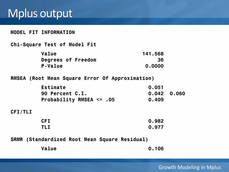
MODEL FIT INFORMATION
Chi-Square Test of Model Fit
Value 141.568Degrees of Freedom 36P-Value 0.0000
RMSEA (Root Mean Square Error Of Approximation)
Estimate 0.05190 Percent C.I. 0.042 0.060Probability RMSEA <= .05 0.409
CFI/TLI
CFI 0.982TLI 0.977
SRMR (Standardized Root Mean Square Residual)
Value 0.106
Mplus output
Growth Modeling in Mplus
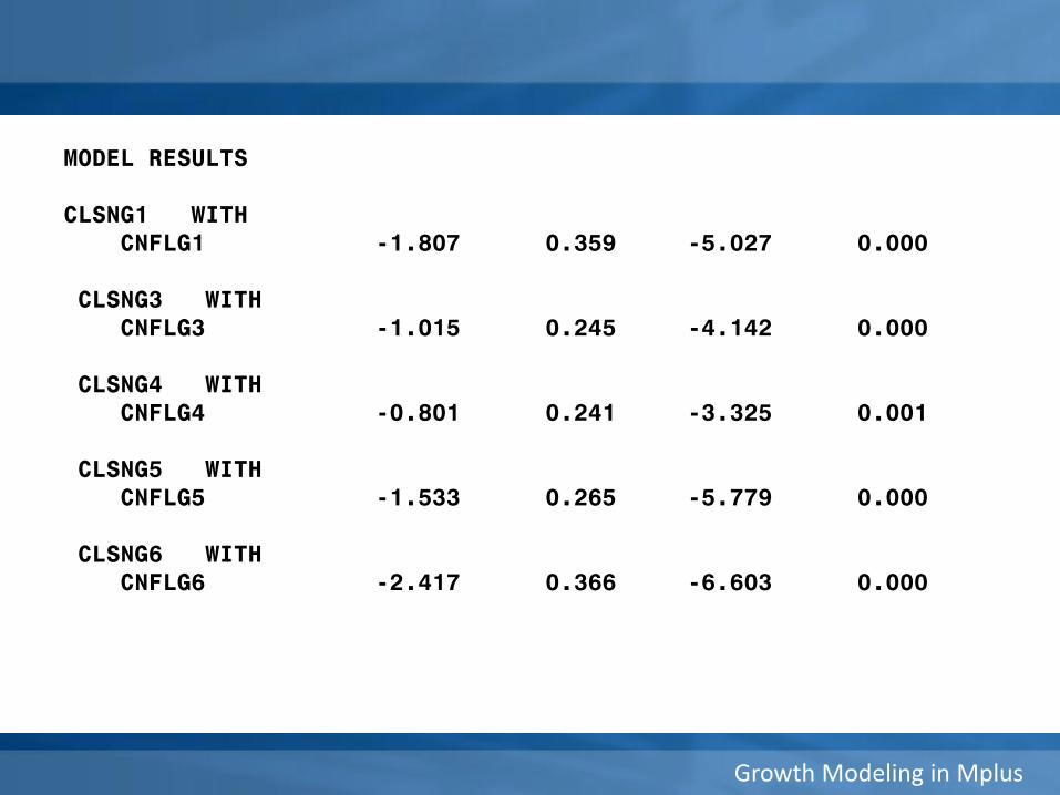
MODEL RESULTS
CLSNG1 WITHCNFLG1 -1.807 0.359 -5.027 0.000
CLSNG3 WITHCNFLG3 -1.015 0.245 -4.142 0.000
CLSNG4 WITHCNFLG4 -0.801 0.241 -3.325 0.001
CLSNG5 WITHCNFLG5 -1.533 0.265 -5.779 0.000
CLSNG6 WITHCNFLG6 -2.417 0.366 -6.603 0.000
Growth Modeling in Mplus
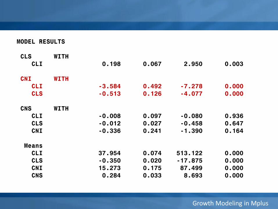
MODEL RESULTS
CLS WITHCLI 0.198 0.067 2.950 0.003
CNI WITHCLI -3.584 0.492 -7.278 0.000CLS -0.513 0.126 -4.077 0.000
CNS WITHCLI -0.008 0.097 -0.080 0.936CLS -0.012 0.027 -0.458 0.647CNI -0.336 0.241 -1.390 0.164
MeansCLI 37.954 0.074 513.122 0.000CLS -0.350 0.020 -17.875 0.000CNI 15.273 0.175 87.499 0.000CNS 0.284 0.033 8.693 0.000
Growth Modeling in Mplus
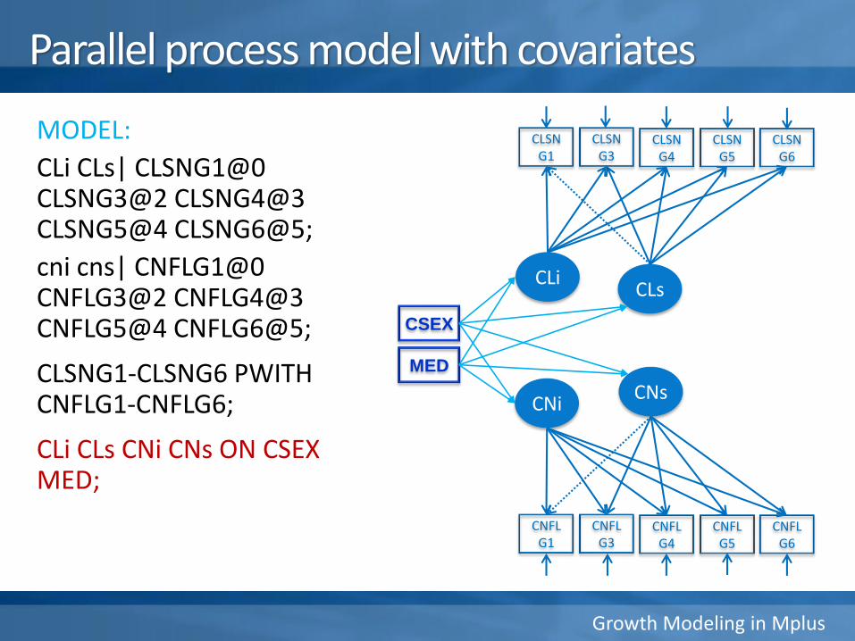
Parallel process model with covariates
CLSN G1
CLSN G3
CLSN G4
CLSN G5
CLiCLs
CLSN G6
MODEL:
CLi CLs| CLSNG1@0 CLSNG3@2 CLSNG4@3 CLSNG5@4 CLSNG6@5;
cni cns| CNFLG1@0 CNFLG3@2 CNFLG4@3 CNFLG5@4 CNFLG6@5;
CLSNG1-CLSNG6 PWITH CNFLG1-CNFLG6;
CLi CLs CNi CNs ON CSEX MED;
CNFL G1
CNFL G3
CNFL G4
CNFL G5
CNiCNs
CNFL G6
CSEX
MED
Growth Modeling in Mplus
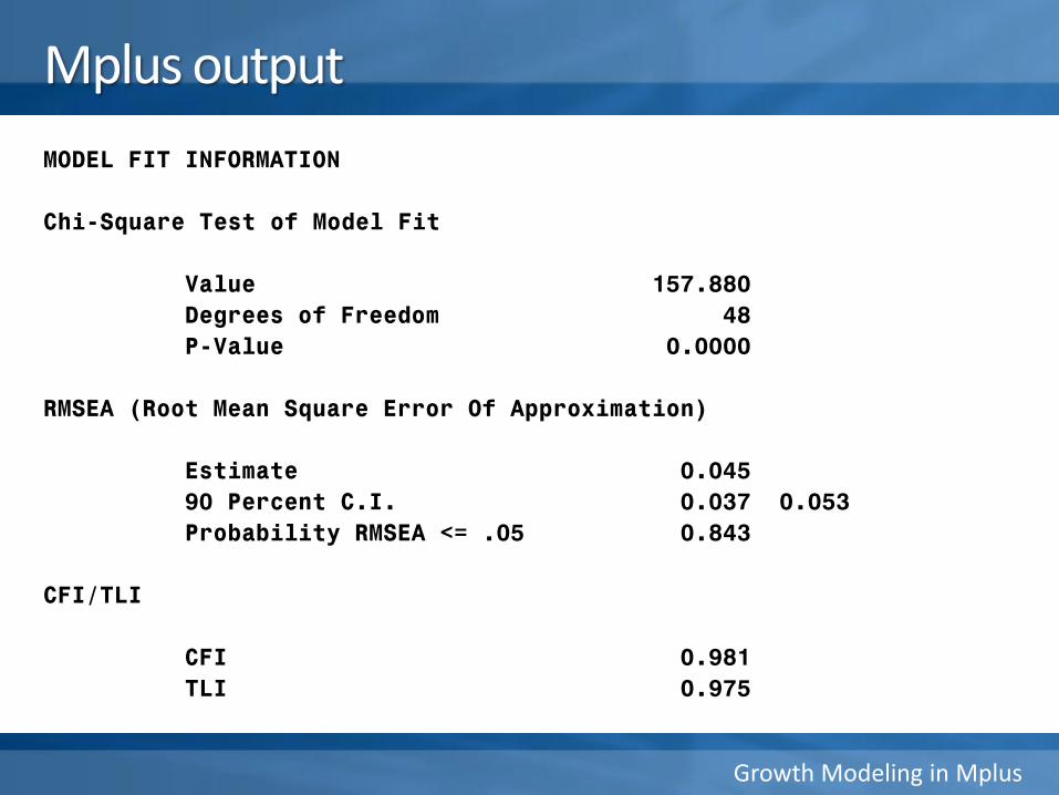
Mplus output
MODEL FIT INFORMATION
Chi-Square Test of Model Fit
Value 157.880
Degrees of Freedom 48
P-Value 0.0000
RMSEA (Root Mean Square Error Of Approximation)
Estimate 0.045
90 Percent C.I. 0.037 0.053
Probability RMSEA <= .05 0.843
CFI/TLI
CFI 0.981
TLI 0.975
Growth Modeling in Mplus
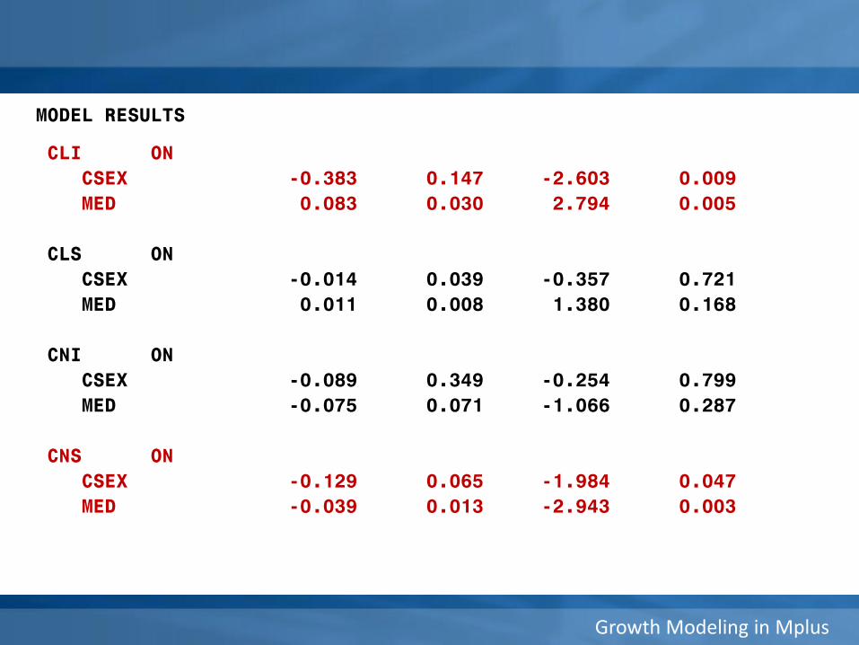
MODEL RESULTS
CLI ON
CSEX -0.383 0.147 -2.603 0.009
MED 0.083 0.030 2.794 0.005
CLS ON
CSEX -0.014 0.039 -0.357 0.721
MED 0.011 0.008 1.380 0.168
CNI ON
CSEX -0.089 0.349 -0.254 0.799
MED -0.075 0.071 -1.066 0.287
CNS ON
CSEX -0.129 0.065 -1.984 0.047
MED -0.039 0.013 -2.943 0.003