INTRODUCTION TO GENETIC EPIDEMIOLOGY …...Introduction to Genetic Epidemiology CHAPTER 3: Different...

INTRODUCTION TO GENETIC EPIDEMIOLOGY

(EPID0754)

Prof. Dr. Dr. K. Van Steen

Introduction to Genetic Epidemiology CHAPTER 3: Different faces of genetic epidemiology

K Van Steen 2

DIFFERENT FACES OF GENETIC EPIDEMIOLOGY

1 Basic epidemiology

1.a Aims of epidemiology

1.b Designs in epidemiology

1.c An overview of measurements in epidemiology

2 Genetic epidemiology

2.a What is genetic epidemiology?

2.b Designs in genetic epidemiology

2.c Study types in genetic epidemiology


K Van Steen 3

3 Phenotypic aggregation within families

3.a Introduction to familial aggregation?

3.b Familial aggregation with quantitative traits

IBD and kinship coefficient

3.c Familial aggregation with dichotomous traits

Relative recurrence risk

3.d Twin studies


K Van Steen 4

4 Segregation analysis

4.a What is segregation analysis?

Modes of inheritance

4.b Classical method for sibships and one locus

Segregation ratios

4.c Likelihood method for pedigrees and one locus

Elston-Stewart algorithm


K Van Steen 5

4.d Variance component modeling: a general framework

Decomposition of variability, major gene, polygenic and mixed models

4.e The ideas of variance component modeling adjusted for binary

traits

Liability threshold models

5 Linkage and association

6 Genetic epidemiology and public health


K Van Steen 6

1 Basic epidemiology

Main references:

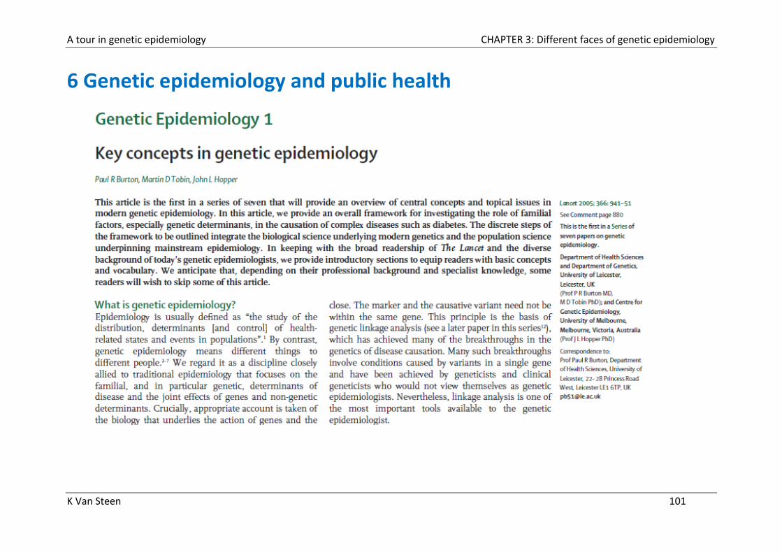
Burton P, Tobin M and Hopper J. Key concepts in genetic epidemiology. The Lancet, 2005

Clayton D. Introduction to genetics (course slides Bristol 2003)

Bonita R, Beaglehole R and Kjellström T. Basic Epidemiology. WHO 2nd edition

URL:

- http://www.dorak.info/


K Van Steen 7

1.a Aims of epidemiology

Epidemiology originates from Hippocrates’ observation more than 2000 years ago that environmental factors influence the occurrence of disease. However, it was not until the nineteenth century that the distribution of disease in specific human population groups was measured to any large extent. This work marked not only the formal beginnings of epidemiology but also some of its most spectacular achievements.

Epidemiology in its modern form is a relatively new discipline and uses quantitative methods to study diseases in human populations, to inform prevention and control efforts.


K Van Steen 8

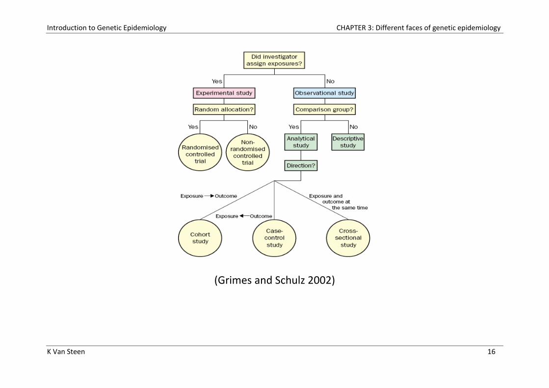
1.b Designs in epidemiology

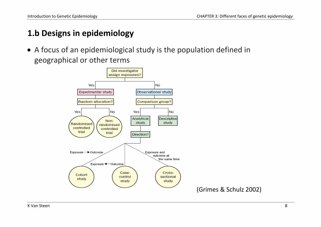
A focus of an epidemiological study is the population defined in geographical or other terms

(Grimes & Schulz 2002)


K Van Steen 9

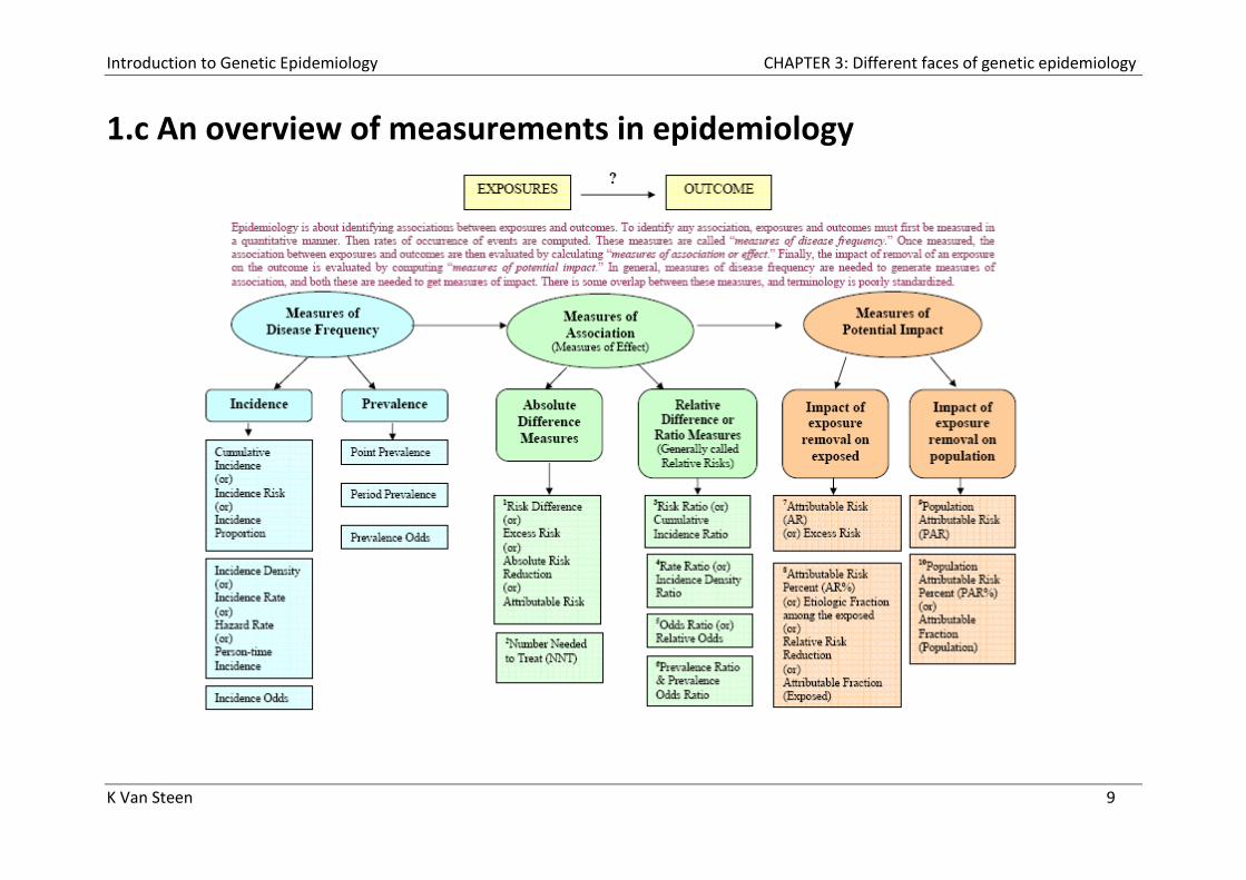
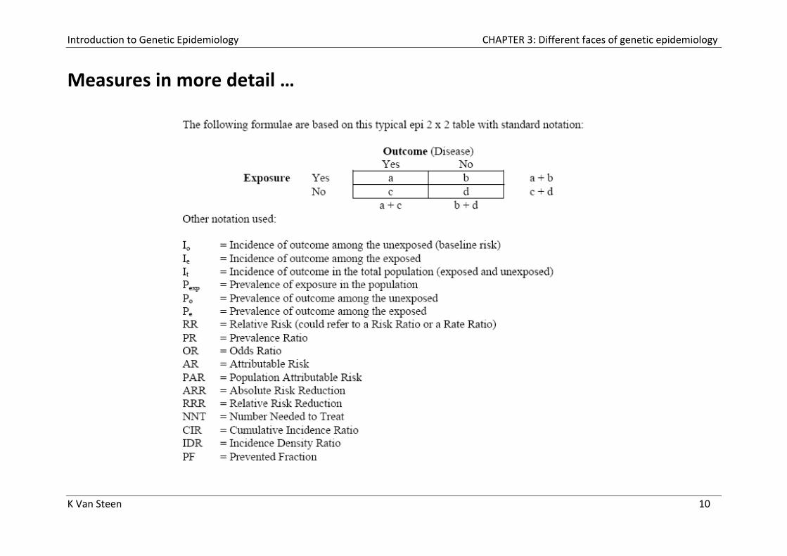
1.c An overview of measurements in epidemiology


K Van Steen 10

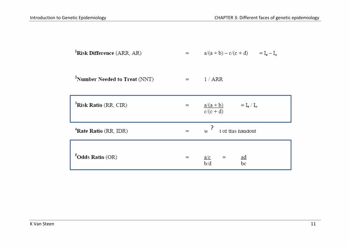
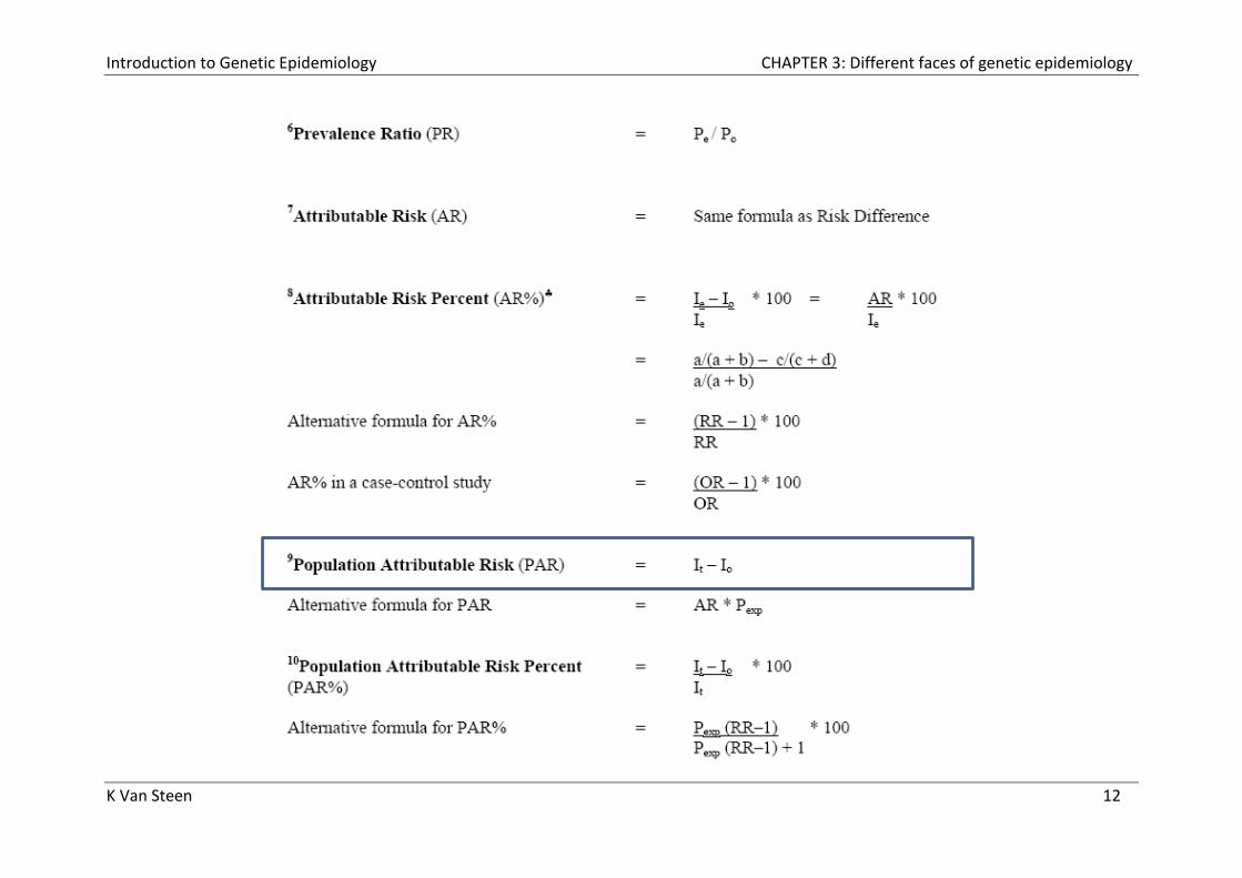
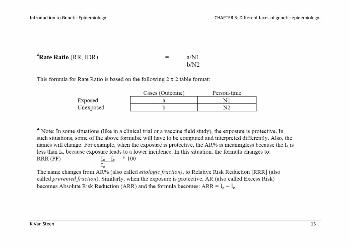
Measures in more detail …


K Van Steen 11

?


K Van Steen 12


K Van Steen 13


K Van Steen 14

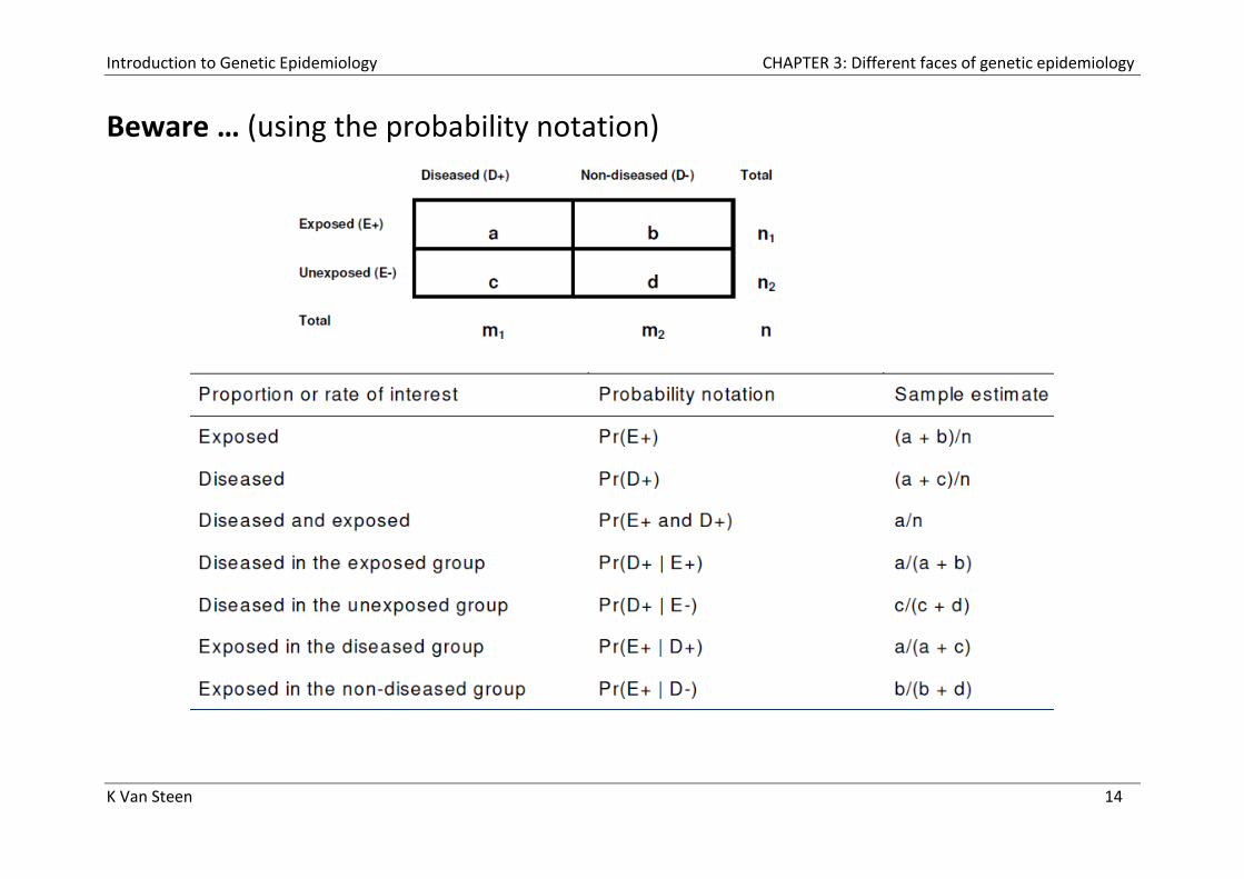
Beware … (using the probability notation)


K Van Steen 15


K Van Steen 16

(Grimes and Schulz 2002)


K Van Steen 17

Summary of most important features by design


K Van Steen 18

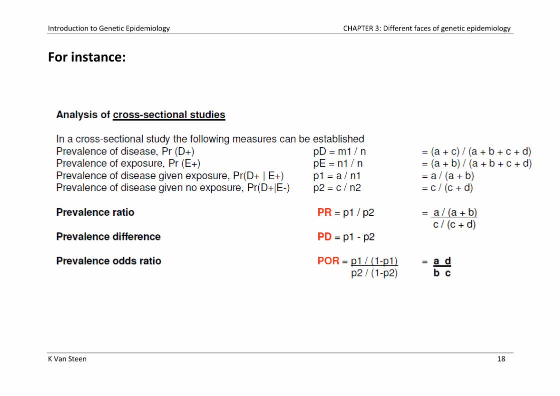
For instance:


K Van Steen 19

Summary of major advantages (bold) and disadvantages


K Van Steen 20

2 Genetic epidemiology

Main references:


Ziegler A. Genetic epidemiology present and future (presentation slides)

URL:


- http://www.answers.com/topic/

- http://www.arbo-zoo.net/_data/ArboConFlu_StudyDesign.pdf

http://www.dorak.info/

http://www.answers.com/topic/


K Van Steen 21

2.a What is genetic epidemiology?

Definitions

Term firstly used by Morton & Chung (1978)

Genetic epidemiology is a science which deals with the etiology, distribution, and control of disease in groups of relatives and with inherited causes of disease in populations . (Morton, 1982).

Genetic epidemiology is the study of how and why diseases cluster in

families and ethnic groups (King et al., 1984)

Genetic epidemiology examines the role of genetic factors, along with the

environmental contributors to disease, and at the same time giving equal attention to the differential impact of environmental agents, non-familial as well as familial, on different genetic backgrounds (Cohen, Am J Epidemiol, 1980)

http://www.amazon.com/exec/obidos/tg/detail/-/380552269X/qid=1101292908/sr=1-1/ref=sr_1_1/104-1935157-9461551?v=glance&s=books


K Van Steen 22

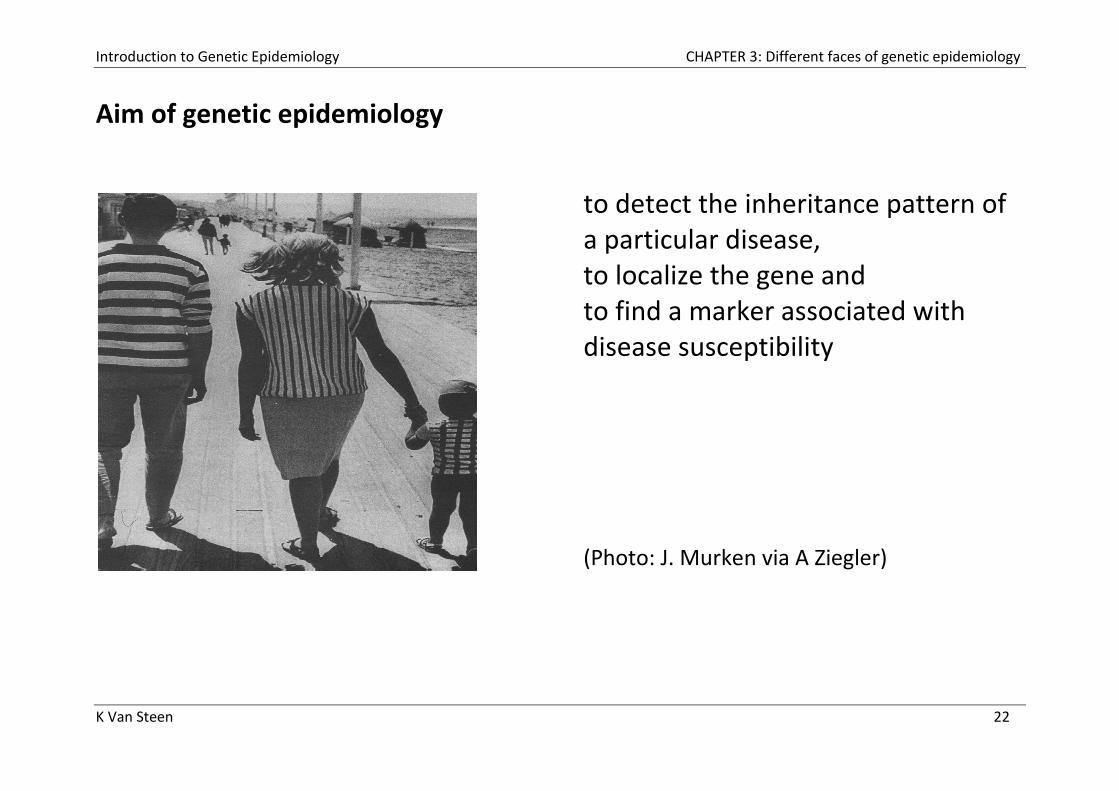
Aim of genetic epidemiology

to detect the inheritance pattern of a particular disease, to localize the gene and to find a marker associated with disease susceptibility (Photo: J. Murken via A Ziegler)

A tour in genetic epidemiology CHAPTER 3: Different faces of genetic epidemiology

K Van Steen 23

X – epidemiology

(Rebbeck TR, Cancer, 1999)


K Van Steen 24

X – epidemiology

Genetic epidemiology is closely allied to both molecular epidemiology and statistical genetics, but these overlapping fields each have distinct emphases, societies and journals.

The phrase "molecular epidemiology" was first coined in 1973 by Kilbourne in an article entitled "The molecular epidemiology of influenza".

The term became more formalised with the formulation of the first book on "Molecular Epidemiology: Principles and Practice" by Schulte and Perera.

Nowadays, molecular epidemiologic studies measure exposure to specific substances (DNA adducts) and early biological response (somatic mutations), evaluate host characteristics (genotype and phenotype) mediating response to external agents, and use markers of a specific effect (like gene expression) to refine disease categories (such as heterogeneity, etiology and prognosis).

http://www.answers.com/topic/molecular-epidemiology-1

http://www.answers.com/topic/population-genetics


K Van Steen 25

X – epidemiology

Genetic epidemiology is closely allied to both molecular epidemiology and statistical genetics, but these overlapping fields each have distinct emphases, societies and journals.

Statistical geneticists are highly trained scientific investigators who are specialists in both statistics and genetics: Statistical geneticists must be able to understand molecular and clinical genetics, as well as mathematics and statistics, to effectively communicate with scientists from these disciplines.

Statistical genetics is a very exciting professional area because it is so new and there is so much demand. It is a rapidly changing field, and there are many fascinating scientific questions that need to be addressed. Additionally, given the interdisciplinary nature of statistical genetics, there are plenty of opportunities to interact with researchers and clinicians in other fields, such as epidemiology, biochemistry, physiology, pathology, evolutionary biology, and anthropology.

http://www.answers.com/topic/molecular-epidemiology-1

http://www.answers.com/topic/population-genetics

http://www.answers.com/topic/fascinating

http://www.answers.com/topic/epidemiology

http://www.answers.com/topic/biochemistry

http://www.answers.com/topic/pathology


K Van Steen 26

X – epidemiology

Just as statistical genetics requires a combination of training in statistics and genetics, genetic epidemiology requires training in epidemiology and genetics. Since both disciplines require knowledge of statistical methods, there is significant overlap.

A primary difference between statistical genetics and genetic epidemiology is that statistical geneticists are often more interested in the development and evaluation of new statistical methods, whereas genetic epidemiologists focus more on the application of statistical methods to biomedical research problems.

A primary difference between genetic and molecular epidemiology is that the first is also concerned with the detection of inheritance patterns.


K Van Steen 27

More recently, the scope of genetic epidemiology has expanded to include common diseases for which many genes each make a smaller contribution (polygenic, multifactorial or multigenic disorders).

This has developed rapidly in the first decade of the 21st century following completion of the Human Genome Project, as advances in genotyping technology and associated reductions in cost has made it feasible to conduct large-scale genome-wide association studies that genotype many thousands of single nucleotide polymorphisms in thousands of individuals.

These have led to the discovery of many genetic polymorphisms that influence the risk of developing many common diseases.


K Van Steen 28

X-epidemiology

In contrast to classic epidemiology, the three main complications in modern genetic epidemiology are

- dependencies, - use of indirect evidence and - complex data sets

Genetic epidemiology is highly dependent on the direct incorporation of family structure and biology. The structure of families and chromosomes leads to major dependencies between the data and thus to customized models and tests. In many studies only indirect evidence can be used, since the disease-related gene, or more precisely the functionally relevant DNA variant of a gene, is not directly observable. In addition, the data sets to be analyzed can be very complex.


K Van Steen 29

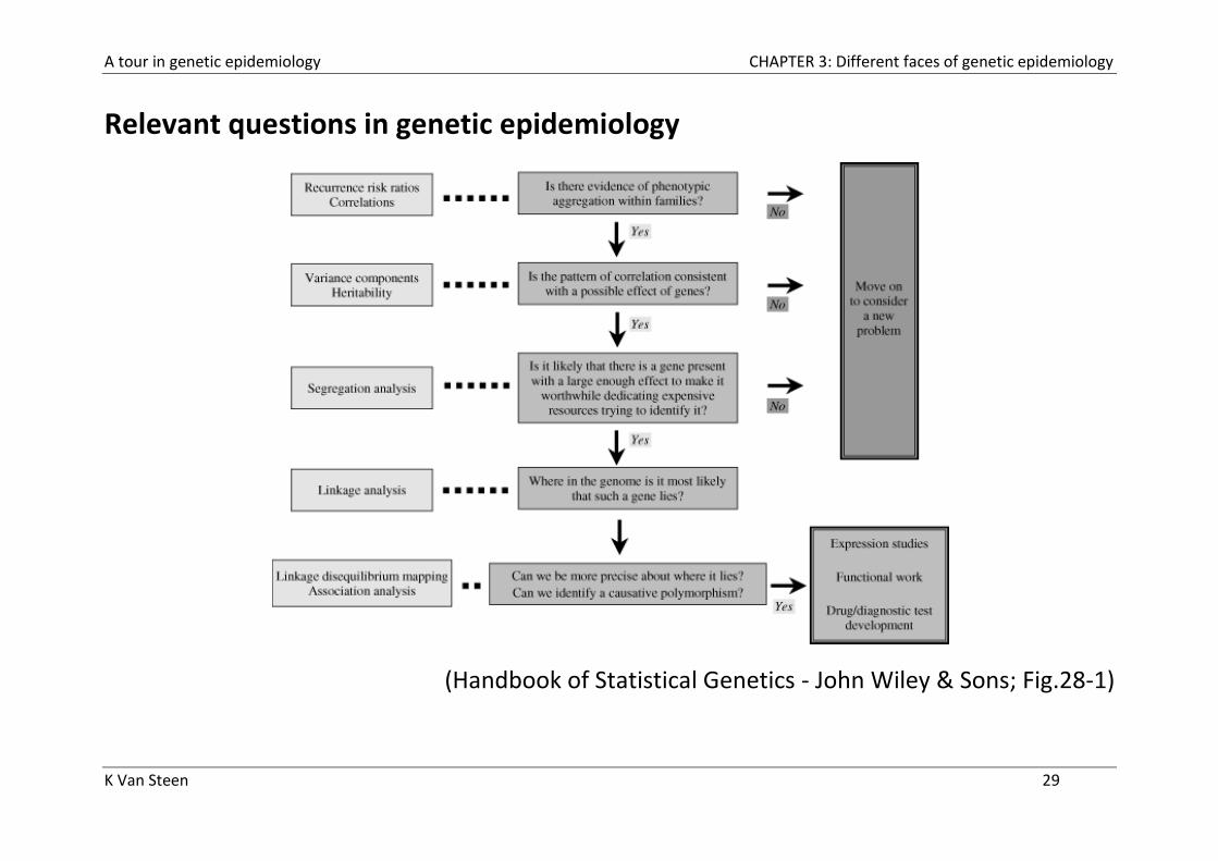
Relevant questions in genetic epidemiology

(Handbook of Statistical Genetics - John Wiley & Sons; Fig.28-1)


K Van Steen 30

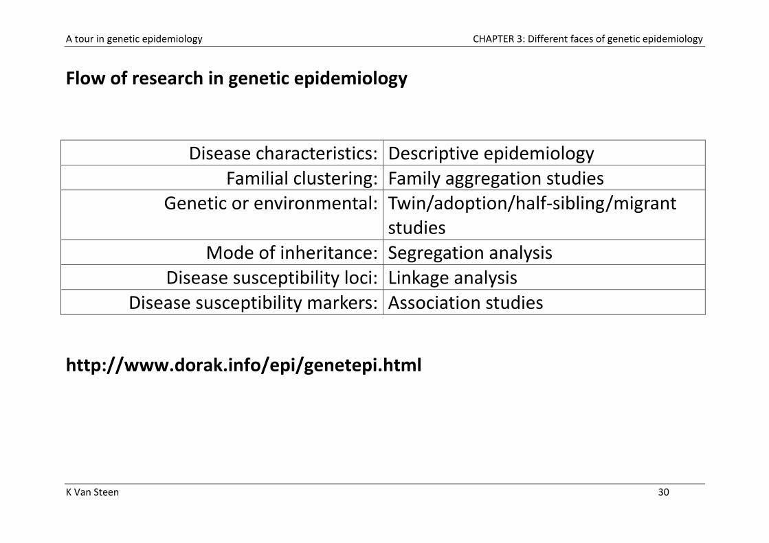
Flow of research in genetic epidemiology

Disease characteristics: Descriptive epidemiology Familial clustering: Family aggregation studies

Genetic or environmental: Twin/adoption/half-sibling/migrant studies

Mode of inheritance: Segregation analysis Disease susceptibility loci: Linkage analysis

Disease susceptibility markers: Association studies

http://www.dorak.info/epi/genetepi.html


K Van Steen 31

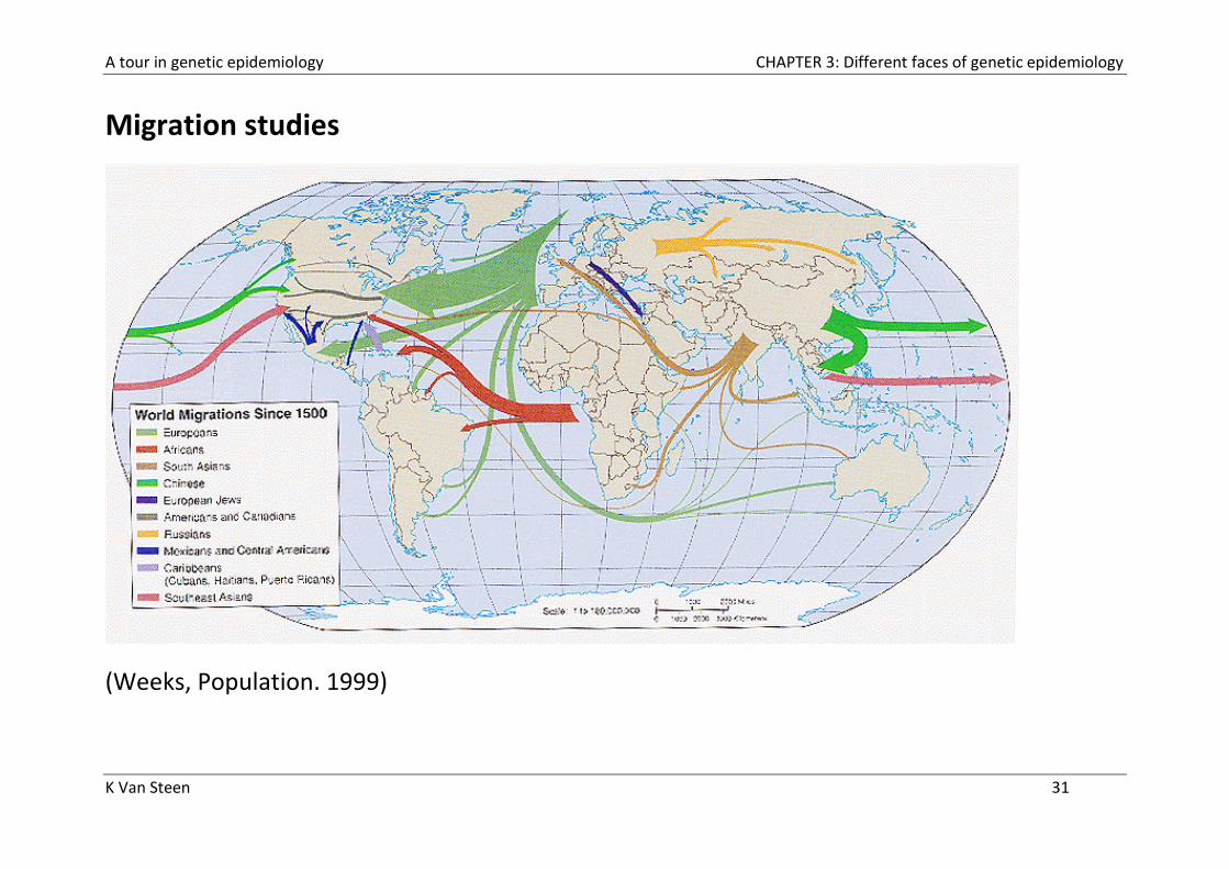
Migration studies

(Weeks, Population. 1999)


K Van Steen 32

Migration studies

As one of the initial steps in the process of genetic epidemiology, one could use information on populations who migrate to countries with different genetic and environmental backgrounds - as well as rates of the disease of interest - than the country they came from.

Here, one compares people who migrate from one country to another with people in the two countries.

If the migrants’ disease frequency does not change –i.e., remains similar to that of their original country, not their new country—then the disease might have genetic components.

If the migrants’ disease frequency does change—i.e., is no longer similar to that of their original country, but now is similar to their new country—then the disease might have environmental components


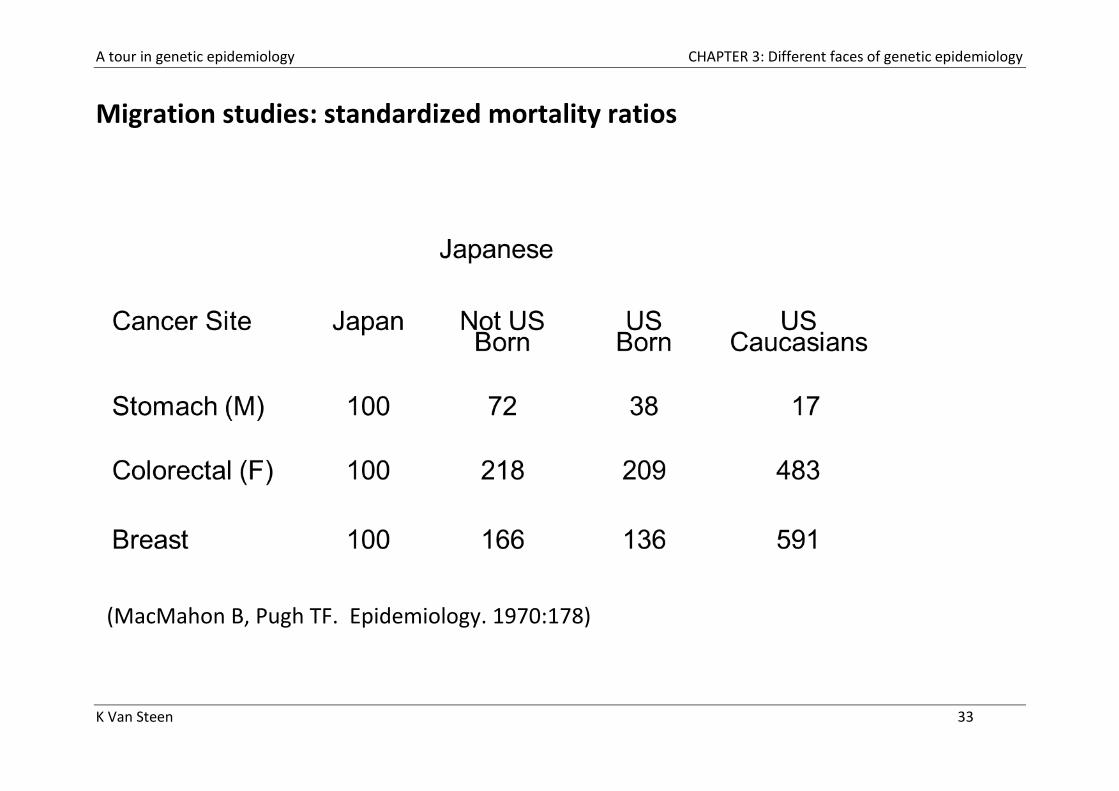
K Van Steen 33

Migration studies: standardized mortality ratios

(MacMahon B, Pugh TF. Epidemiology. 1970:178)


K Van Steen 34

Genetic research paradigm


K Van Steen 35

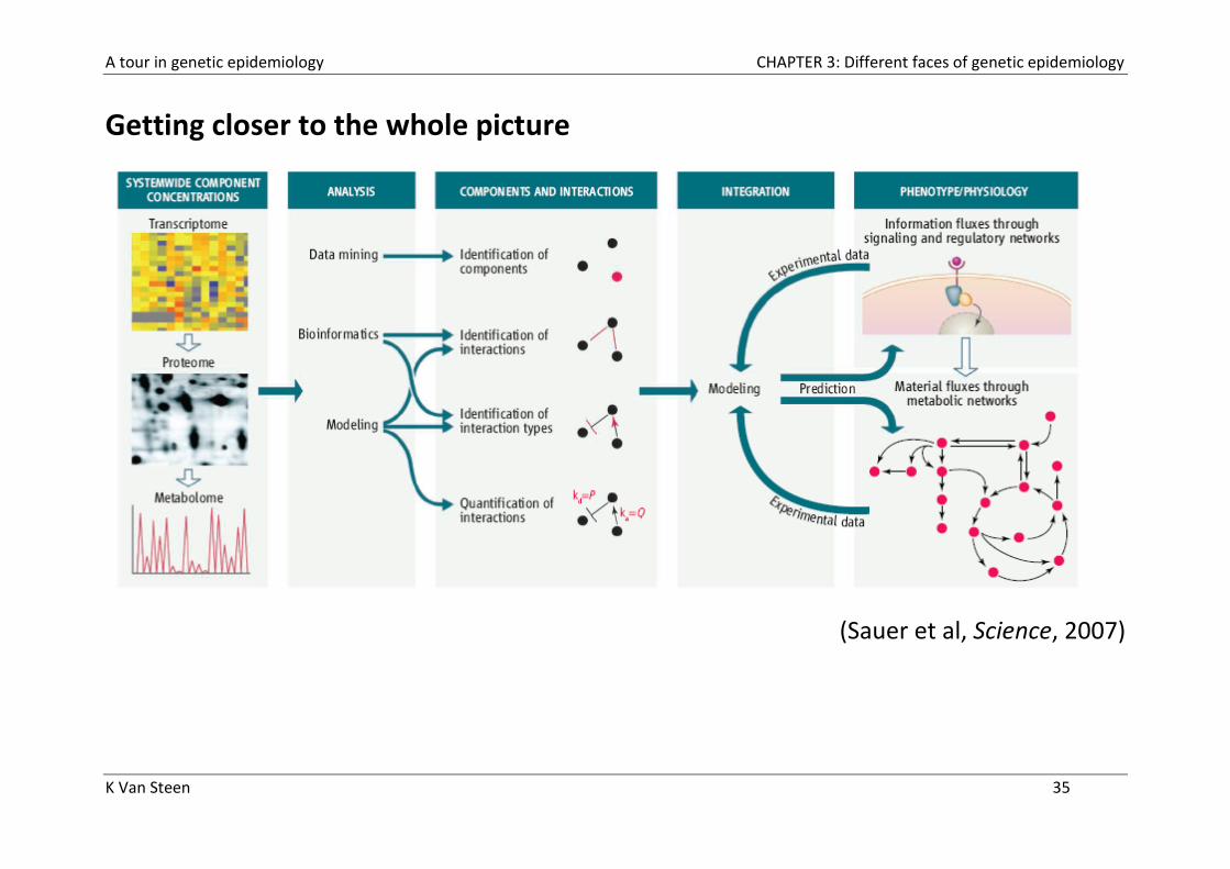
Getting closer to the whole picture

(Sauer et al, Science, 2007)


K Van Steen 36

Recent success stories of genetics and genetic epidemiology research

Gene expression profiling to assess prognosis and guide therapy, e.g. breast cancer

Genotyping for stratification of patients according to risk of disease, e.g. myocardial infarction

Genotyping to elucidate drug response, e.g. antiepileptic agents

Designing and implementing new drug therapies, e.g. imatinib for hypereosinophilic syndrome

Functional understanding of disease causing genes, e.g. obesity

(Guttmacher & Collins, N Engl J Med, 2003)


K Van Steen 37

2.b Designs in genetic epidemiology

The samples needed for genetic epidemiology studies may be

nuclear families (index case and parents),

affected relative pairs (sibs, cousins, any two members of the family),

extended pedigrees,

twins (monozygotic and dizygotic) or

unrelated population samples.


K Van Steen 38

2.c Study types in genetic epidemiology

Main methods in genetic epidemiology

Genetic risk studies:

- What is the contribution of genetics as opposed to environment to the

trait? Requires family-based, twin/adoption or migrant studies.

Segregation analyses:

- What does the genetic component look like (oligogenic 'few genes

each with a moderate effect', polygenic 'many genes each with a small

effect', etc)?

- What is the model of transmission of the genetic trait? Segregation

analysis requires multigeneration family trees preferably with more

than one affected member.


K Van Steen 39

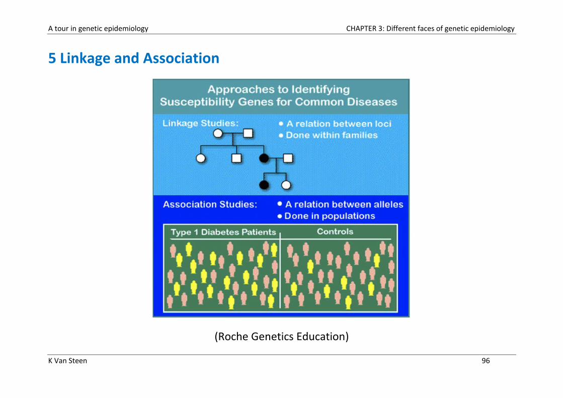
Linkage studies:

- What is the location of the disease gene(s)? Linkage studies screen the

whole genome and use parametric or nonparametric methods such as

allele sharing methods {affected sibling-pairs method} with no

assumptions on the mode of inheritance, penetrance or disease allele

frequency (the parameters). The underlying principle of linkage studies

is the cosegregation of two genes (one of which is the disease locus).

Association studies:

- What is the allele associated with the disease susceptibility? The

principle is the coexistence of the same marker on the same

chromosome in affected individuals (due to linkage disequilibrium).

Association studies may be family-based (TDT) or population-based.

Alleles or haplotypes may be used. Genome-wide association studies

(GWAS) are increasing in popularity.


K Van Steen 40

3 Familial aggregation of a phenotype

Main references:


Thomas D. Statistical methods in genetic epidemiology. Oxford University Press 2004

Laird N and Cuenco KT. Regression methods for assessing familial aggregation of disease.

Stats in Med 2003


URL:



K Van Steen 41

3.a Introduction to familial aggregation

What is familial aggregations?

Consensus on a precise definition of familial aggregation is lacking

The heuristic interpretation is that aggregation exists when cases of disease

appear in families more often than one would expect if diseased cases were

spread uniformly and randomly over individuals.

The assessment of familial aggregation of disease is often regarded as the

initial step in determining whether or not there is a genetic basis for

disease.

Absence of any evidence for familial aggregation casts strong doubt on a

genetic component influencing disease, especially when environmental

factors are included in the analysis.


K Van Steen 42

What is familial aggregation? (continued)

Actual approaches for detecting aggregation depend on the nature of the

phenotype, but the common factor in existing approaches is that they are

taken without any specific genetic model in mind.

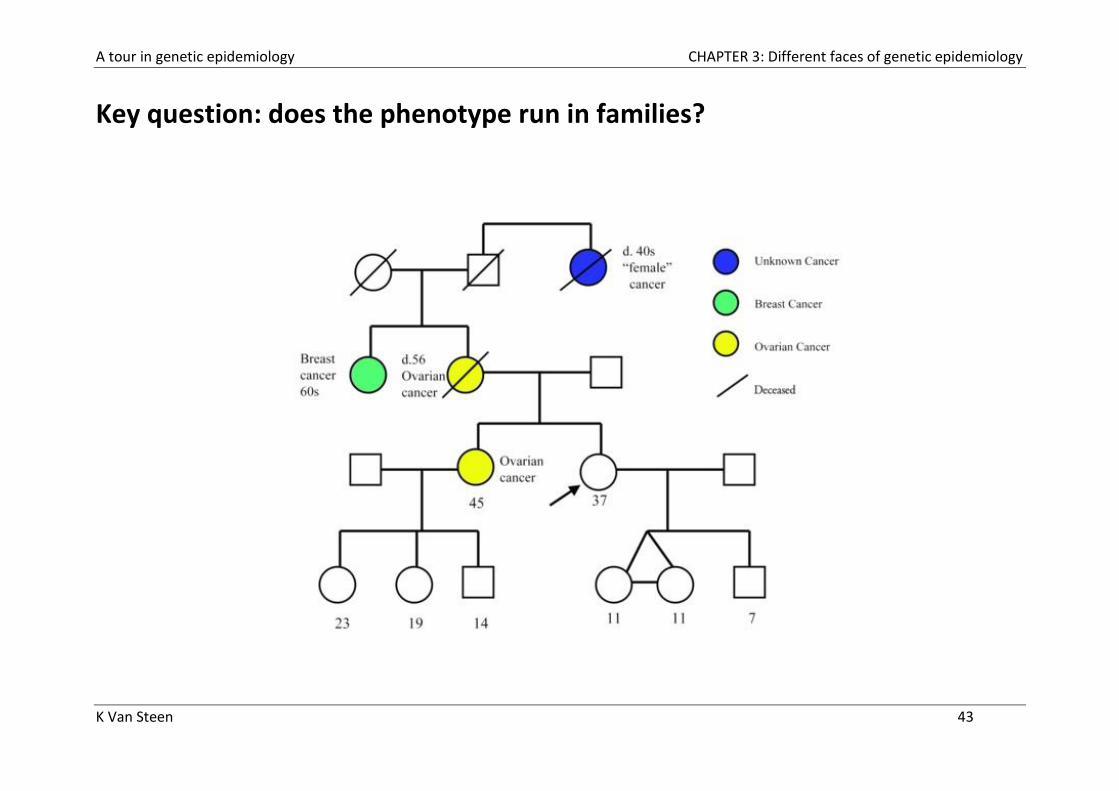
The basic design of familial aggregation studies typically involves sampling

families

In most places there is no natural sampling frame for families, so individuals

are selected in some way and then their family members are identified. The

individual who caused the family to be identified is called the proband.


K Van Steen 43

Key question: does the phenotype run in families?


K Van Steen 44

Define the phenotype !!!

Gleason DF. In Urologic Pathology: The Prostate. 1977; 171-198


K Van Steen 45

3.b Familial aggregation with quantitative traits

Proband selection

For a continuous trait a random series of probands from the general

population may be enrolled, together with their family members.


K Van Steen 46

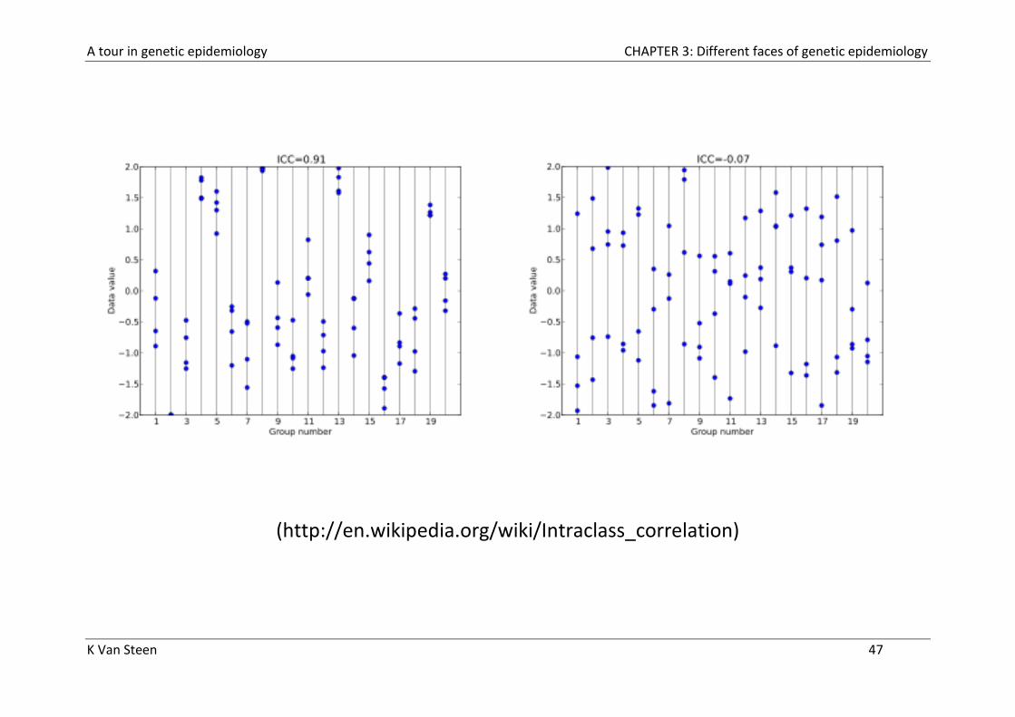
Correlations between trait values among family members

For quantitative traits, such as blood pressure, familial aggregation can be

assessed using a correlation or covariance-based measure

For instance, the so-called intra-family correlation coefficient (ICC)

- It describes how strongly units in the same group resemble each other

- ICC can be interpreted as the proportion of the total variability in a

phenotype that can reasonably be attributed to real variability between

families

- Techniques such as linear regression and mulitilevel modelling analysis of variance are useful to derive estimates

- Non-random ascertainment can seriously bias an ICC.

Alternatively, familial correlation coefficients are computed as in the

programme FCOR within the Statistical Analysis for Genetic Epidemiology

(SAGE) software package


K Van Steen 47

(http://en.wikipedia.org/wiki/Intraclass_correlation)

http://en.wikipedia.org/wiki/File:ICC-example2.svg

http://en.wikipedia.org/wiki/File:ICC-example1.svg


K Van Steen 48

3.c Familial aggregation with dichotomous traits

Proband selection

It is a misconception that probands always need to have the disease of

interest.

In general, the sampling procedure based on proband selection closely

resembles the case-control sampling design, for which exposure is assessed

by obtaining data on disease status of relatives, usually first-degree

relatives, of the probands. This selection procedure is particularly practical

when disease is relatively rare.


K Van Steen 49

Two main streams in analysis

In a retrospective type of analysis, the outcome of interest is disease in the

proband. Disease in the relatives serves to define the exposure.

Recent literature focuses on a prospective type of analysis, in which disease

status of the relatives is considered the outcome of interest and is

conditioned on disease status in the proband.


K Van Steen 50

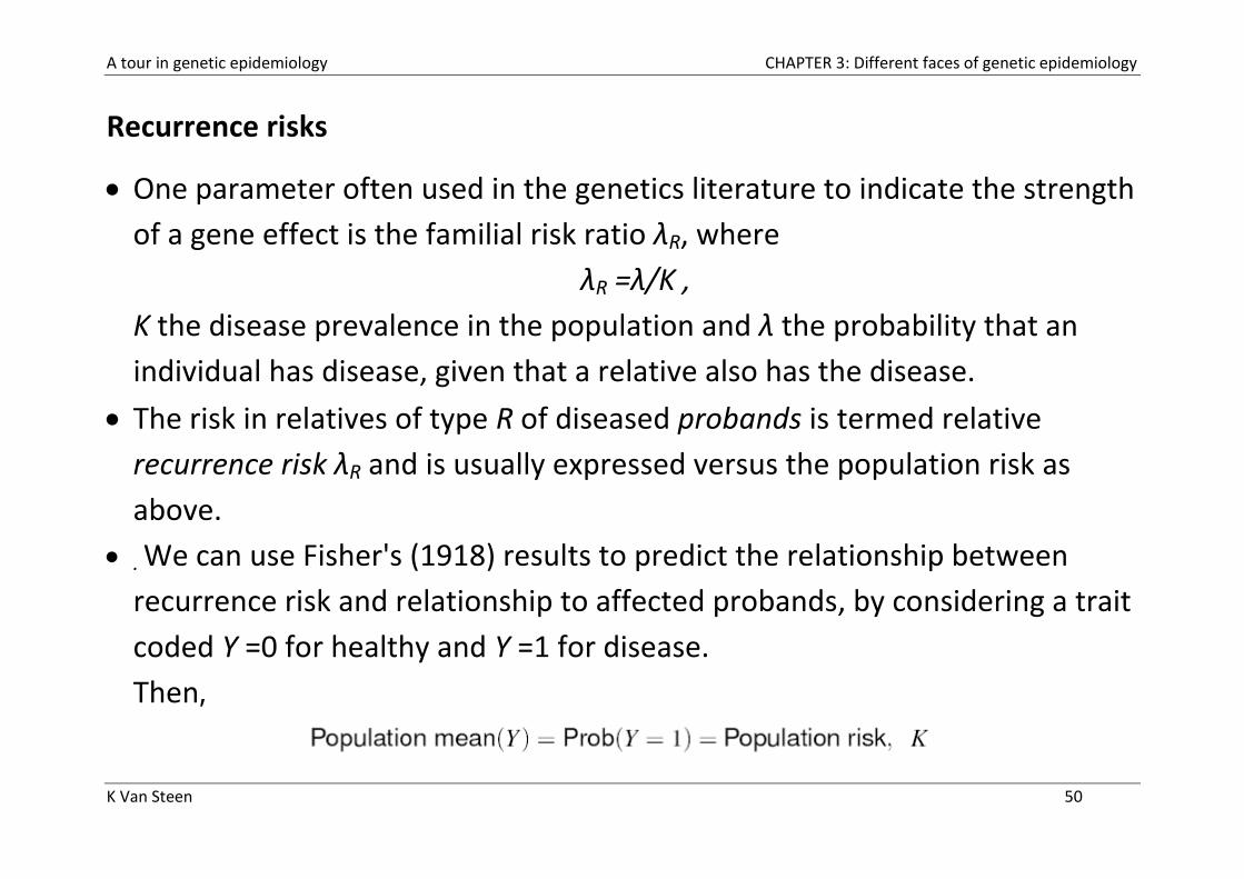
Recurrence risks

One parameter often used in the genetics literature to indicate the strength

of a gene effect is the familial risk ratio λR, where

λR =λ/K ,

K the disease prevalence in the population and λ the probability that an

individual has disease, given that a relative also has the disease.

The risk in relatives of type R of diseased probands is termed relative

recurrence risk λR and is usually expressed versus the population risk as

above.

. We can use Fisher's (1918) results to predict the relationship between

recurrence risk and relationship to affected probands, by considering a trait

coded Y =0 for healthy and Y =1 for disease.

Then,


K Van Steen 51

Recurrence risks (continued)

An alternative algebraic expression for the covariance is

with Mean(Y1Y2) the probability that both relatives are affected. From this we

derive for the familial risk ratio λ, defined before:

It is intuitively clear (and it can be shown formally) that the covariance

between Y1 and Y2 depends on the type of relationship (the so-called kinship

coefficient φ (see later)

- Regression methods may be used for assessing familial aggregation of

diseases, using logit link functions


K Van Steen 52

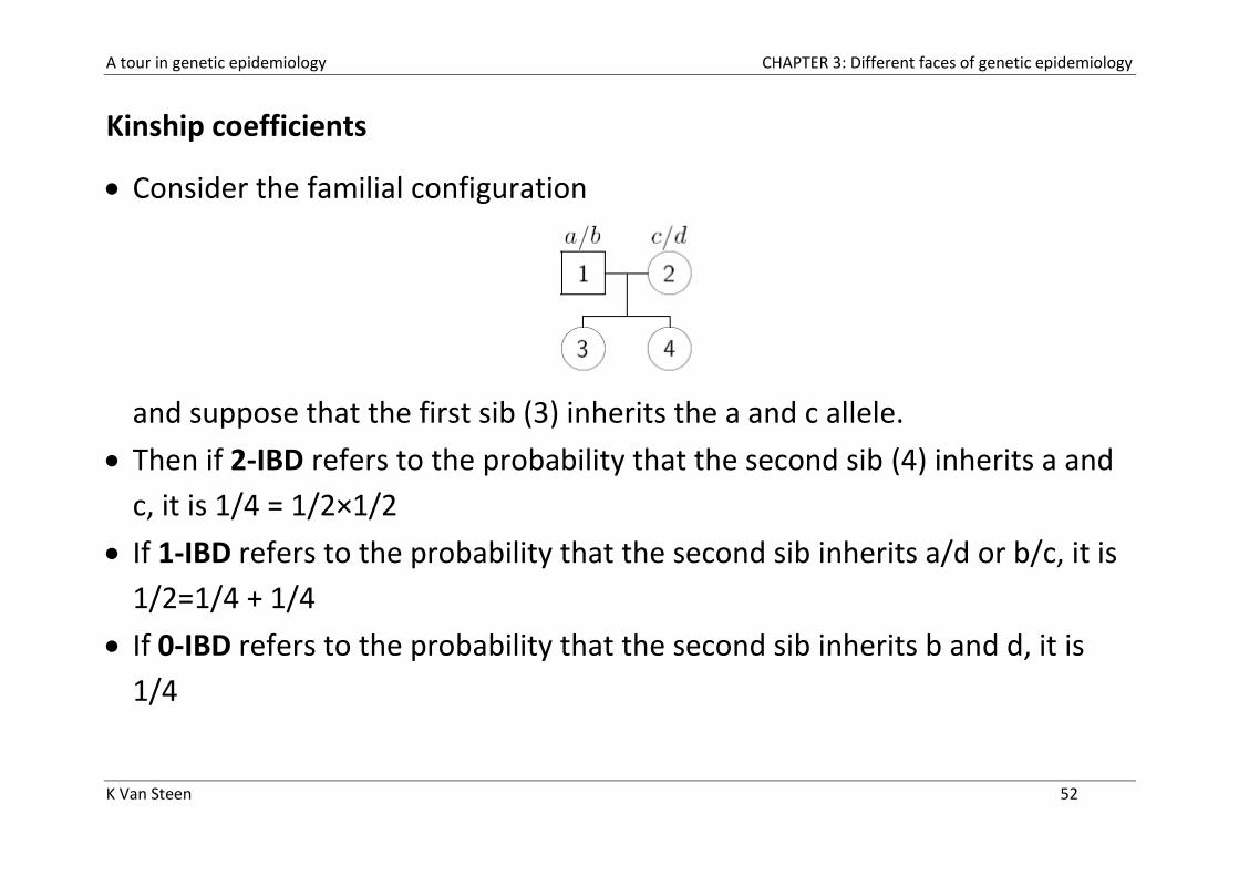
Kinship coefficients

Consider the familial configuration

and suppose that the first sib (3) inherits the a and c allele.

Then if 2-IBD refers to the probability that the second sib (4) inherits a and

c, it is 1/4 = 1/2×1/2

If 1-IBD refers to the probability that the second sib inherits a/d or b/c, it is

1/2=1/4 + 1/4

If 0-IBD refers to the probability that the second sib inherits b and d, it is

1/4


K Van Steen 53

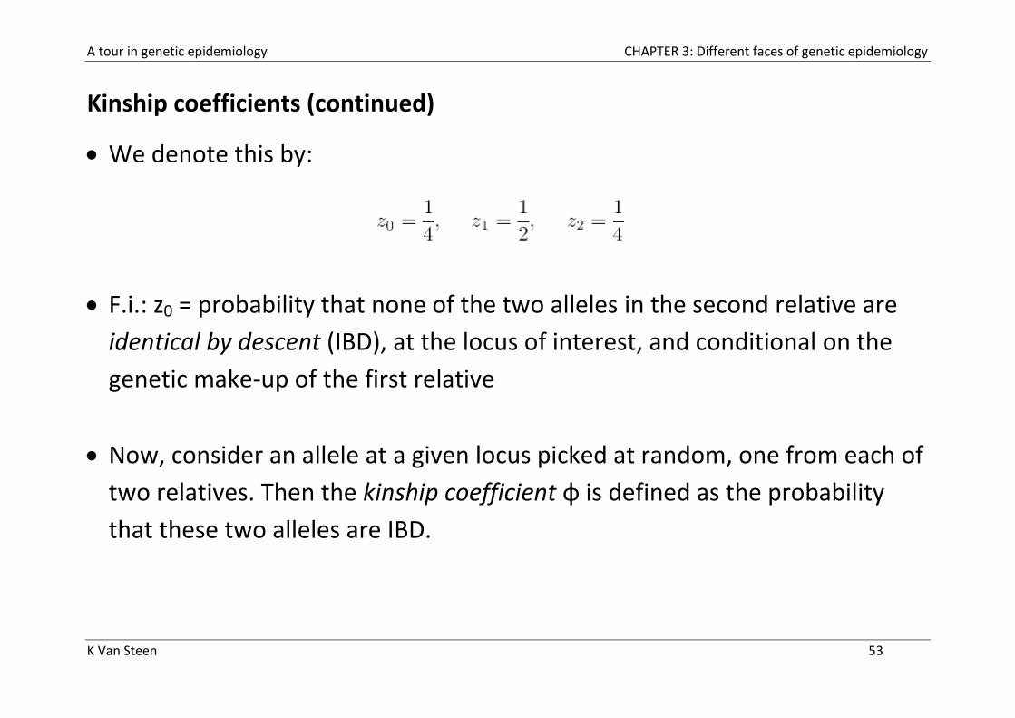
Kinship coefficients (continued)

We denote this by:

F.i.: z0 = probability that none of the two alleles in the second relative are

identical by descent (IBD), at the locus of interest, and conditional on the

genetic make-up of the first relative

Now, consider an allele at a given locus picked at random, one from each of

two relatives. Then the kinship coefficient φ is defined as the probability

that these two alleles are IBD.


K Van Steen 54

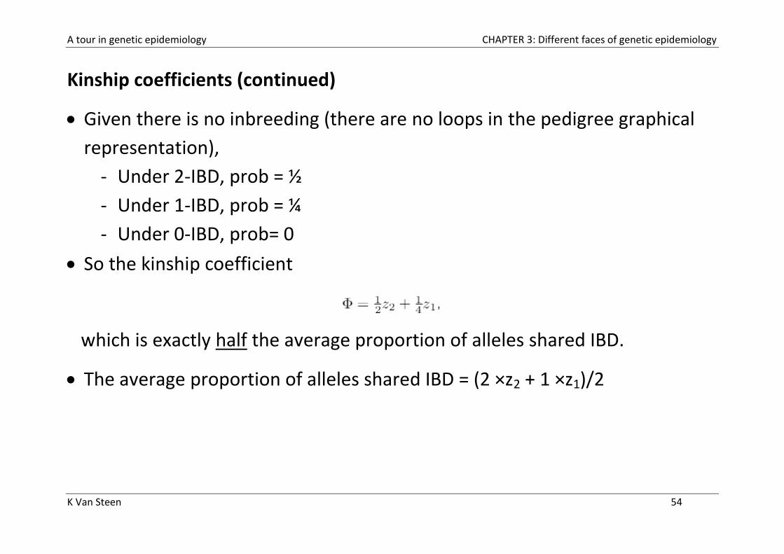
Kinship coefficients (continued)

Given there is no inbreeding (there are no loops in the pedigree graphical

representation),

- Under 2-IBD, prob = ½

- Under 1-IBD, prob = ¼

- Under 0-IBD, prob= 0

So the kinship coefficient

which is exactly half the average proportion of alleles shared IBD.

The average proportion of alleles shared IBD = (2 ×z2 + 1 ×z1)/2


K Van Steen 55

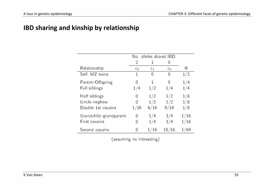
IBD sharing and kinship by relationship


K Van Steen 56

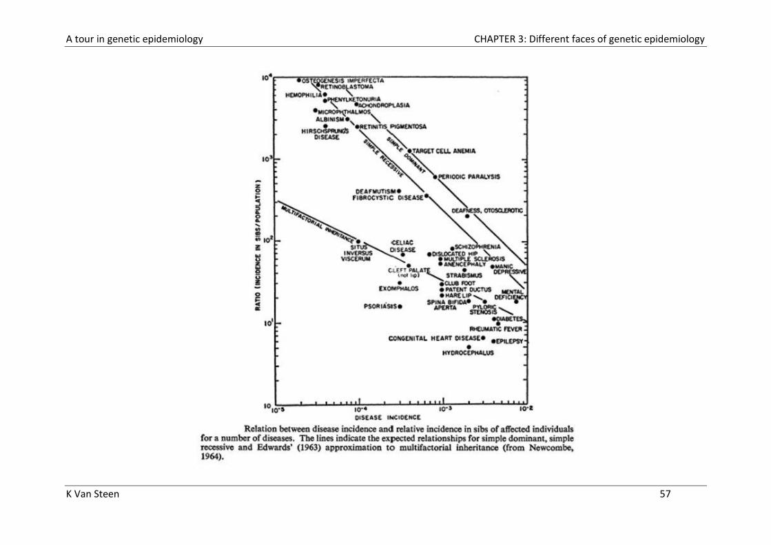
Interpretation of values of relative recurrence risk

Examples for λS = ratio of risk in sibs compared with population risk.

- cystic fibrosis: the risk in sibs = 0.25 and the risk in the population =

0.0004, and therefore λS =500

- Huntington disease: the risk in sibs = 0.5 and the risk in the population =

0.0001, and therefore λS =5000

Higher value indicates greater proportion of risk in family compared with

population.

The relative recurrence risk increases with

- Increasing genetic contribution

- Decreasing population prevalence


K Van Steen 57


K Van Steen 58

Interpretation of values of relative recurrence risk (continued)

The presence of familial aggregation can be due to many factors, including

shared family environment.

Hence, familial aggregation alone is not sufficient to demonstrate a genetic

basis for the disease.

Here, variance components modeling may come into play to explain the

pattern of familial aggregation and to derive estimates of heritability (see

next section: segregation analysis)

When trying to decipher the importance of genetic versus environmental

factors, twin designs are extremely useful:


K Van Steen 59

3. e Twin studies

Environment versus genetics


K Van Steen 60

Contribution of twins to the study of complex traits and diseases

Concordance is defined as is the probability that a pair of individuals will

both have a certain characteristic, given that one of the pair has the

characteristic.

- For example, twins are concordant when both have or both lack a given

trait

One can distinguish between pairwise concordance and proband wise

concordance:

- Pairwise concordance is defined as C/(C+D), where C is the number of

concordant pairs and D is the number of discordant pairs

- For example, a group of 10 twins have been pre-selected to have one

affected member (of the pair). During the course of the study four

other previously non-affected members become affected, giving a

pairwise concordance of 4/(4+6) or 4/10 or 40%.


K Van Steen 61

Contribution of twins to the study of complex traits and diseases

(continued)

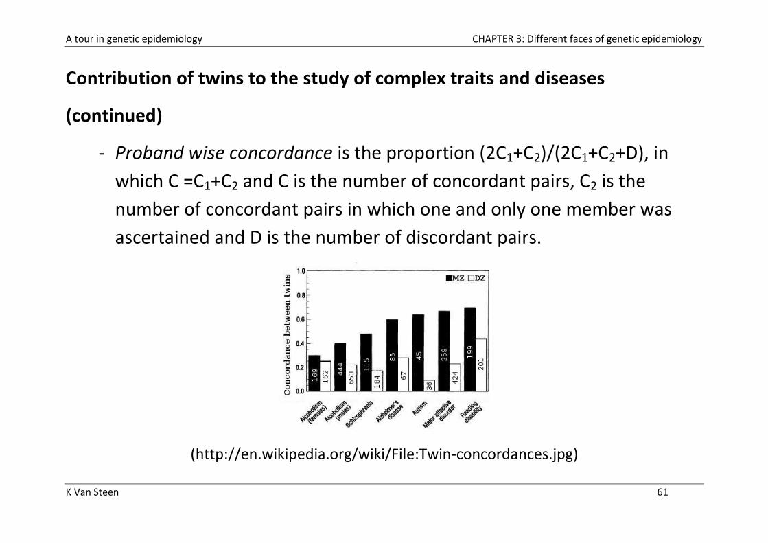
- Proband wise concordance is the proportion (2C1+C2)/(2C1+C2+D), in

which C =C1+C2 and C is the number of concordant pairs, C2 is the

number of concordant pairs in which one and only one member was

ascertained and D is the number of discordant pairs.

(http://en.wikipedia.org/wiki/File:Twin-concordances.jpg)

http://upload.wikimedia.org/wikipedia/en/c/cf/Twin-concordances.jpg


K Van Steen 62

Some details about twin studies

The basic logic of the twin study can be understood with very little

mathematics beyond an understanding of correlation and the concept of

variance.

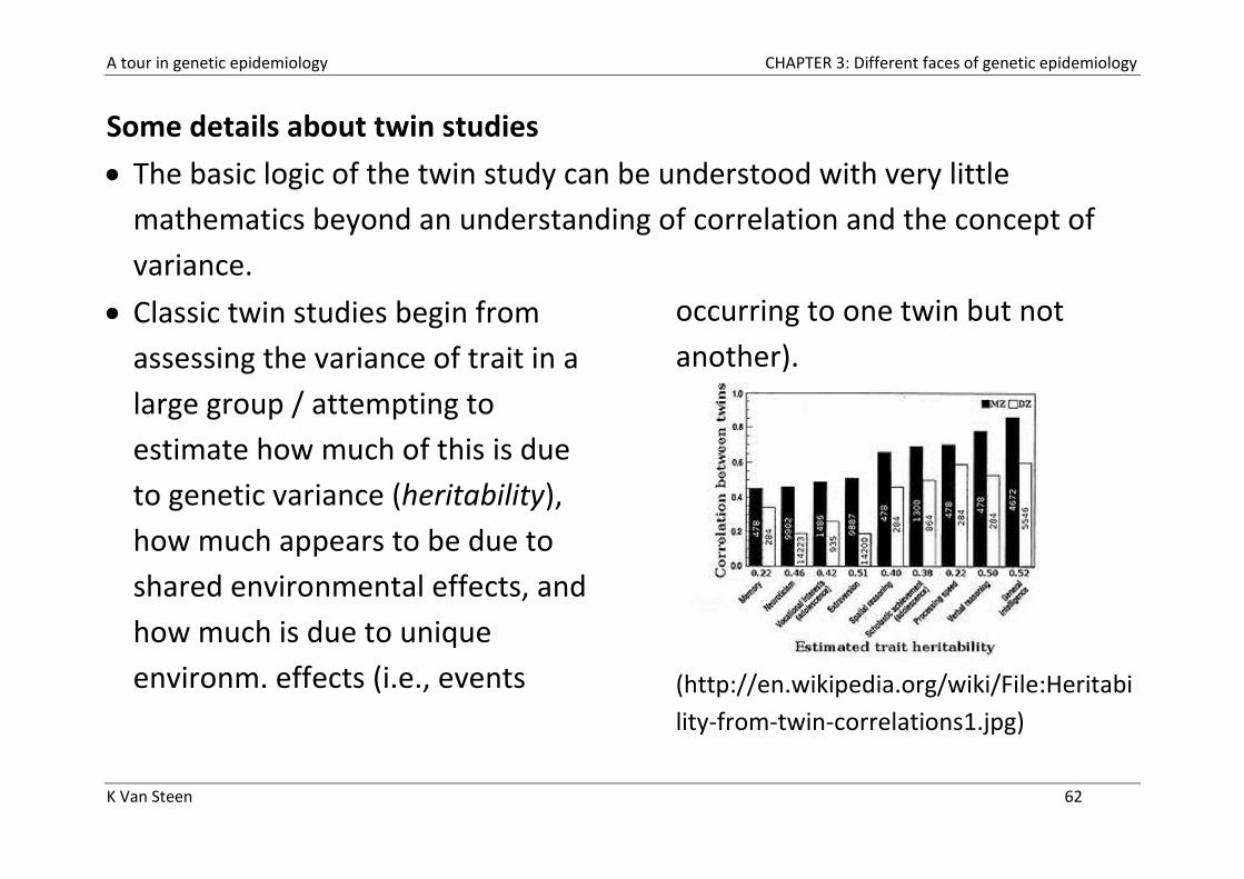
Classic twin studies begin from

assessing the variance of trait in a

large group / attempting to

estimate how much of this is due

to genetic variance (heritability),

how much appears to be due to

shared environmental effects, and

how much is due to unique

environm. effects (i.e., events

occurring to one twin but not

another).

(http://en.wikipedia.org/wiki/File:Heritabi

lity-from-twin-correlations1.jpg)

http://en.wikipedia.org/wiki/Correlation

http://en.wikipedia.org/wiki/Variance

http://en.wikipedia.org/wiki/Heritability

http://en.wikipedia.org/wiki/File:Heritability-from-twin-correlations1.jpg


K Van Steen 63

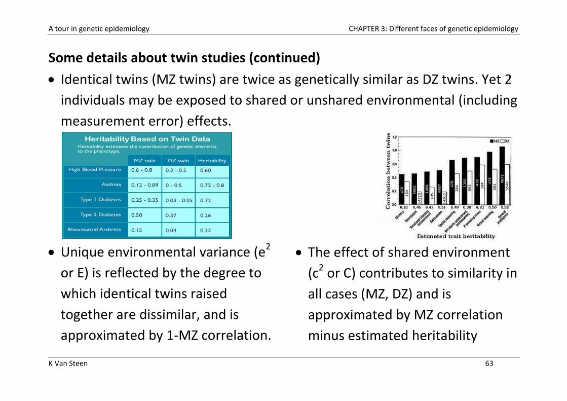
Some details about twin studies (continued)

Identical twins (MZ twins) are twice as genetically similar as DZ twins. Yet 2

individuals may be exposed to shared or unshared environmental (including

measurement error) effects.

Unique environmental variance (e2

or E) is reflected by the degree to

which identical twins raised

together are dissimilar, and is

approximated by 1-MZ correlation.

The effect of shared environment

(c2 or C) contributes to similarity in

all cases (MZ, DZ) and is

approximated by MZ correlation

minus estimated heritability

http://en.wikipedia.org/wiki/File:Heritability-from-twin-correlations1.jpg


K Van Steen 64


How to estimate heritability?

- Given the ACE model, researchers can determine what proportion of

variance in a trait is heritable, versus the proportions which are due to

shared environment or unshared environment, for instance using

programs that implement structural equation models (SEM) - e.g.,

available in the freeware Mx software .

- The A in the ACE model stands for the additive genetic effect size (cfr.

additive genetic variance, narrow heritability). It is also possible to

examine non-additive genetics effects (often denoted D for dominance

(ADE model).

Consequently, heritability (h2) is approximately twice the difference

between MZ and DZ twin correlations.

http://en.wikipedia.org/wiki/ADE_model


K Van Steen 65


Monozygous (MZ) twins raised in a family share both 100% of their genes,

and all of the shared environment (actually, this is often just an

assumption). Any differences arising between them in these circumstances

are random (unique).

- The correlation we observe between MZ twins therefore provides an

estimate of A + C .

Dizygous (DZ) twins have a common shared environment, and share on

average 50% of their genes.

- So the correlation between DZ twins is a direct estimate of ½A + C .


K Van Steen 66

Different studies may lead to quite different heritability estimates!

(Maher 2008)


K Van Steen 67

4 Segregation analysis

Main references:


Thomas D. Statistical methods in genetic epidemiology. Oxford University Press 2004


URL:


Additional reading:

Ginsburg E and Livshits G. Segregation analysis of quantitative traits, Annals of human

biology, 1999

http://www.dorak.info/


K Van Steen 68

4.a What is a segregation analysis?

Harry Potter’s pedigree


K Van Steen 69

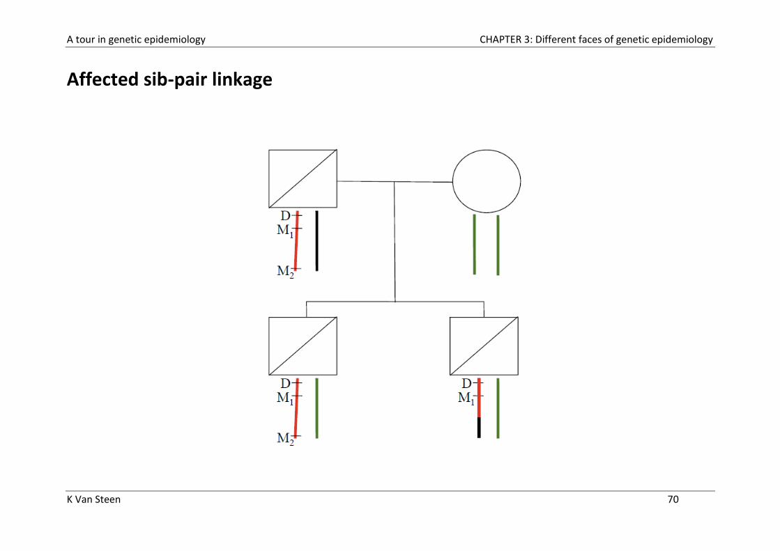
Definition of segregation analysis

Segregation analysis is a statistical technique that attempts to explain the

causes of family aggregation of disease.

It aims to determine the transmission pattern of the trait within families

and to test this pattern against predictions from specific genetic models:

- Dominant? Recessive? Co-dominant? Additive?

Segregation analysis entails fitting a variety of models (both genetic and

non-genetic; major genes or multiple genes/polygenes) to the data

obtained from families and evaluating the results to determine which

model best fits the data.

As in aggregation studies, families are often ascertained through probands

This information is useful in parametric linkage analysis, which assumes a

defined model of inheritance


K Van Steen 70

Affected sib-pair linkage


K Van Steen 71

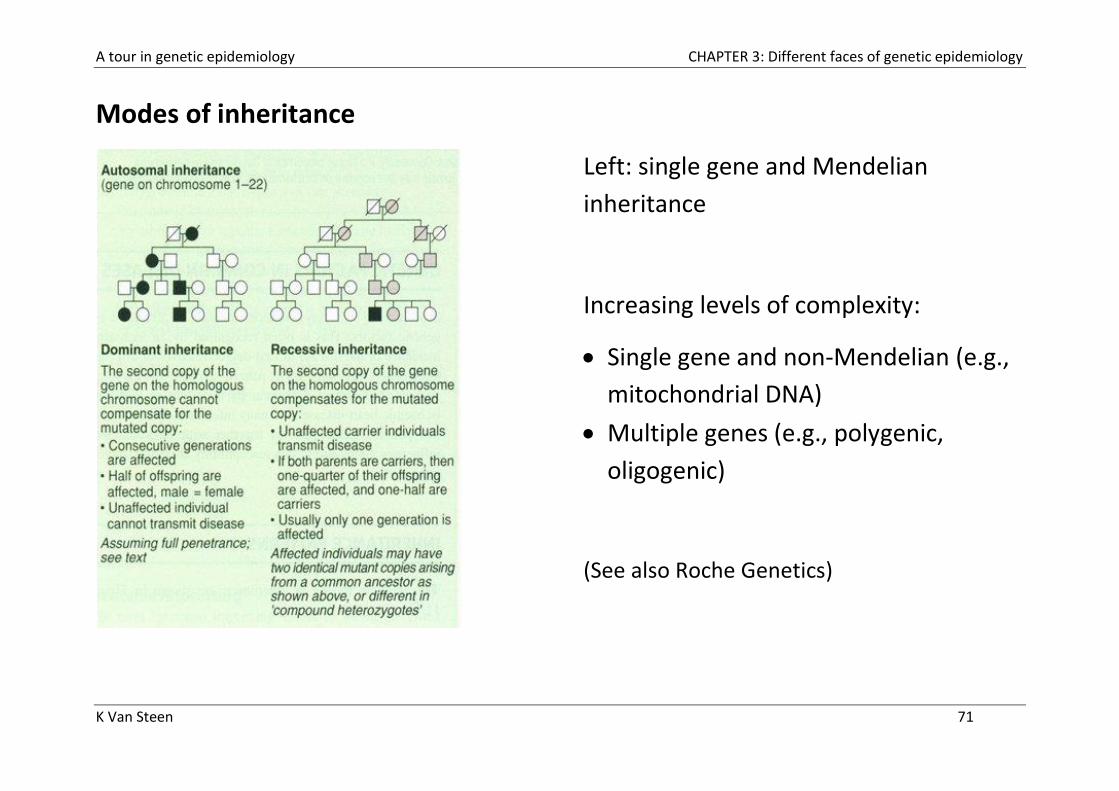
Modes of inheritance

Left: single gene and Mendelian

inheritance

Increasing levels of complexity:

Single gene and non-Mendelian (e.g.,

mitochondrial DNA)

Multiple genes (e.g., polygenic,

oligogenic)

(See also Roche Genetics)


K Van Steen 72

Mitochondrial DNA

Mitochondrial DNA (mtDNA) is the DNA located in the mitochondria,

structures within eukaryotic cells that convert the chemical energy from

food into a form that cells can use, adenosine triphosphate (ATP). Most of

the rest of human DNA present in eukaryotic cells can be found in the cell

nucleus. In most species, including humans, mtDNA is inherited solely from

the mother (i.e., maternally inherited).

In humans, mitochondrial DNA can be regarded as the smallest

chromosome coding for only 37 genes and containing only about 16,600

base pairs.

Human mitochondrial DNA was the first significant part of the human

genome to be sequenced.

http://en.wikipedia.org/wiki/DNA

http://en.wikipedia.org/wiki/Mitochondrion

http://en.wikipedia.org/wiki/Eukaryotic

http://en.wikipedia.org/wiki/Adenosine_triphosphate

http://en.wikipedia.org/wiki/Cell_nucleus

http://en.wikipedia.org/wiki/Cell_nucleus

http://en.wikipedia.org/wiki/Chromosome

http://en.wikipedia.org/wiki/Human_mitochondrial_DNA

http://en.wikipedia.org/wiki/Human_genome

http://en.wikipedia.org/wiki/Human_genome


K Van Steen 73

Distinguishing between different types of genetic diseases

Monogenic diseases are those in which defects in a single gene produce

disease. Often these disease are severe and appear early in life, e.g.,

cystic fibrosis. For the population as a whole, they are relatively rare. In a

sense, these are pure genetic diseases: They do not require any

environmental factors to elicit them. Although nutrition is not involved in

the causation of monogenic diseases, these diseases can have

implications for nutrition. They reveal the effects of particular proteins or

enzymes that also are influenced by nutritional factors

(http://www.utsouthwestern.edu)


K Van Steen 74

Oligogenic diseases are conditions produced by the combination of two,

three, or four defective genes. Often a defect in one gene is not enough

to elicit a full-blown disease; but when it occurs in the presence of other

moderate defects, a disease becomes clinically manifest. It is the

expectation of human geneticists that many chronic diseases can be

explained by the combination of defects in a few (major) genes.

A third category of genetic disorder is polygenic disease. According to the

polygenic hypothesis, many mild defects in genes conspire to produce

some chronic diseases. To date the full genetic basis of polygenic diseases

has not been worked out; multiple interacting defects are highly

complex!!!

(http://www.utsouthwestern.edu)


K Van Steen 75

Complex diseases refer to conditions caused by many contributing factors.

Such a disease is also called a multifactorial disease.

- Some disorders, such as sickle cell anemia and cystic fibrosis, are

caused by mutations in a single gene.

- Common medical problems such as heart disease, diabetes, and obesity

likely associated with the effects of multiple genes in combination with

lifestyle and environmental factors, all of them possibly interacting.

http://ghr.nlm.nih.gov/condition=cysticfibrosis


K Van Steen 76

Two terms frequently used in a segregation analysis

So the aim of segregation analysis is to find evidence for the existence of a

major gene for the phenotype under investigation and to estimate the

corresponding mode of inheritance, or to reject this assumption

The segregation ratios are the predictable proportions of genotypes and

phenotypes in the offspring of particular parental crosses. e.g. 1 AA : 2 AB :

1 BB following a cross of AB X AB

Segregation ratio distortion is a departure from expected segregation

ratios. The purpose of segregation analysis is to detect significant

segregation ratio distortion. A significant departure would suggest one of

our assumptions about the model wrong.


K Van Steen 77

4.b Classical method for sibships and one locus

Steps of a simple segregation analysis

Identify mating type(s) where the trait is expected to segregate in the

offspring.

Sample families with the given mating type from the population.

Sample and score the children of sampled families.

Estimate segregation ratio or test H0: “expected segregation ratio” (e.g.,

hypothesizing a particular mode

of inheritance) .


K Van Steen 78

Example: Autosomal dominant

Data and hypothesis:

Obtain a random sample of matings between

affected (Dd) and unaffected (dd) individuals.

Sample n of their offspring and find that r are

affected with the disease (i.e. Dd).

H0: proportion of affected offspring is 0.5


K Van Steen 79

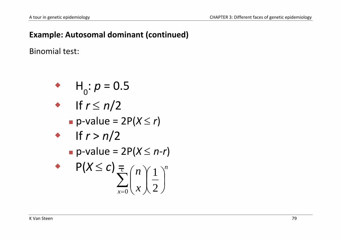
Example: Autosomal dominant (continued)

Binomial test:

H0: p = 0.5

If r n/2 p-value = 2P(X r)

If r > n/2 p-value = 2P(X n-r)

P(X c) =

observe 29

c

x

n

x

n

0 2

1


K Van Steen 80

4.c Likelihood method for pedigrees and one locus

Segregation analysis in practice

For more complicated structures, segregation models are generally fitted

using the method of maximum likelihood. In particular, the parameters of

the model are fitted by finding the values that maximize the probability

(likelihood) of the observed data.

The essential elements of (this often complex likelihood) are

- the penetrance function (i.e., Prob(Disease | Genotype))

- the population genotype

- the transmission probabilities within families

- the method of ascertainment


K Van Steen 81

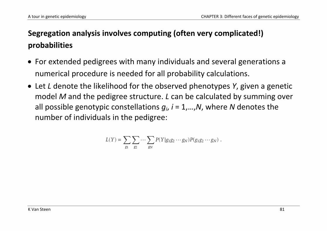
Segregation analysis involves computing (often very complicated!)

probabilities

For extended pedigrees with many individuals and several generations a

numerical procedure is needed for all probability calculations.

Let L denote the likelihood for the observed phenotypes Y, given a genetic model M and the pedigree structure. L can be calculated by summing over all possible genotypic constellations gi, i = 1,…,N, where N denotes the number of individuals in the pedigree:


K Van Steen 82

It is assumed that the phenotype of an individual is independent of the other pedigree members given its genotype.

Widely used in segregation analysis is the Elston–Stuart algorithm (Elston and Stuart 1971), a recursive formula for the computation of the likelihood L given as

(Bickeböller – Genetic Epidemiology)

The Elston-Stewart peeling algorithm involves starting at the bottom of a

pedigree and computing the probability of the parent’s genotypes, given

their phenotypes and the offspring’s phenotypes, and working up from

there, at each stage using the genotype probabilities that have been

computed at lower levels of the pedigree


K Van Steen 83

The notation for the formula is as follows: N denotes the number of individuals in the pedigree. N1 denotes the number of founder individuals in the pedigree. Founders are individuals without specified parents in the pedigree. In general, these are the members of the oldest generation and married-in spouses.N2 denotes the number of non-founder individuals in the pedigree, such that N = N1 + N2. gi, i = 1,…,N, denote the genotype of the ith individual of the pedigree.

The parameters of the genetic model M fall into three groups: (1) The genotype distribution P(gk), k = 1,…,N1, for the founders is determined by population parameters and often Hardy–Weinberg equilibrium is assumed. (2) The transmission probabilities for the transmission from parents to offspring τ(gm|gm1, gm2), where m1 and m2 are the parents of m, are needed for all non-founders in the pedigree. It is assumed that transmissions to different offspring are independent given the parental genotypes and that transmissions of one parent to an offspring are independent of the transmission of the other parent. Thus, transmission probabilities can be parametrized by the product of the individual transmissions. Under Mendelian segregation the transmission probabilities for parental transmission are τ(S1| S1 S1) = 1; τ(S1| S1 S2) = 0.5 and τ(S1| S2 S2) = 0. (3) The penetrances f (gi), i = 1,…,N, parametrize the genotype-phenotype correlation for each individual i.


K Van Steen 84

4.d Variance component modeling; a general framework

Introduction

The extent to which any identified familial aggregation is caused by genes,

can be estimated by a biologically rational model that specifies how

precisely a trait is modulated by the effect of one or more genes.

One of the most common such models is the additive model:

- a given allele at a given locus adds a constant to, or subtracts a constant

from, the expected value of the trait

Here, no information about genotypes or measured environmental

determinants is required! Hence, no blood needs to be taken for DNA

analysis.

(Burton et al, The Lancet, 2005)


K Van Steen 85

Dissecting the genetic variance

In an “analysis of variance” framework:

- The additive component of variance is the variance explained by a

model in which maternal and paternal alleles have simple additive

effects on the mean trait value.

- The dominance component represents residual genetic variance not

explained by a simple sum of effects

In 1918, Fisher established the relationship between the covariance in

trait values between two relatives and their relatedness

The resulting correlation matrix can be analyzed by variance components

or path analysis techniques to estimate the proportion of variance due to

shared environmental and genetic influences.


K Van Steen 86

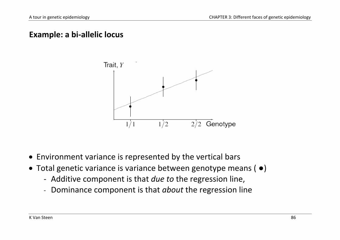
Example: a bi-allelic locus

Environment variance is represented by the vertical bars

Total genetic variance is variance between genotype means ( ●) - Additive component is that due to the regression line, - Dominance component is that about the regression line


K Van Steen 87

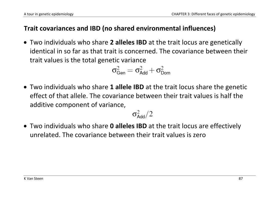
Trait covariances and IBD (no shared environmental influences)

Two individuals who share 2 alleles IBD at the trait locus are genetically identical in so far as that trait is concerned. The covariance between their trait values is the total genetic variance

Two individuals who share 1 allele IBD at the trait locus share the genetic

effect of that allele. The covariance between their trait values is half the additive component of variance,

Two individuals who share 0 alleles IBD at the trait locus are effectively

unrelated. The covariance between their trait values is zero


K Van Steen 88

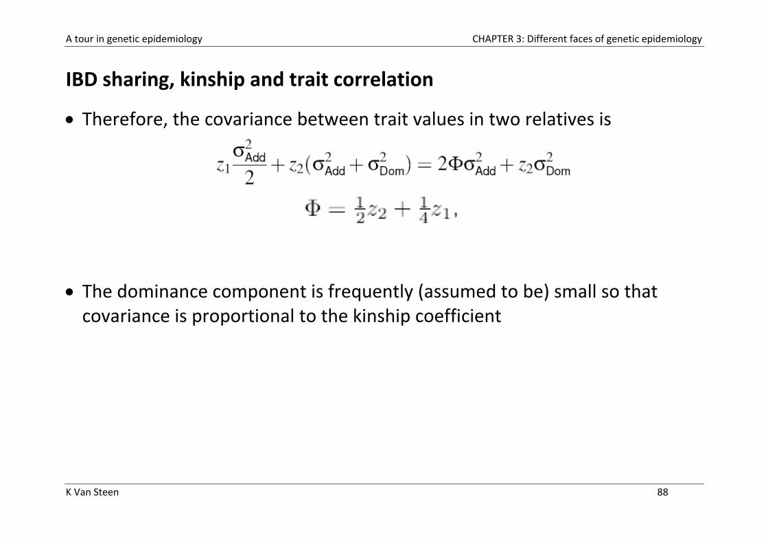
IBD sharing, kinship and trait correlation

Therefore, the covariance between trait values in two relatives is

The dominance component is frequently (assumed to be) small so that covariance is proportional to the kinship coefficient


K Van Steen 89

Single major locus

If inheritance of the trait were due to a single major locus, the bivariate distribution for two relatives would be a mixture of circular clouds of points - Spacing of cloud centres

depends on additive and dominance effects

- Marginal distributions depend on allele frequency

- Tendency to fall along diagonals depends on IBD status (hence on relationship


K Van Steen 90

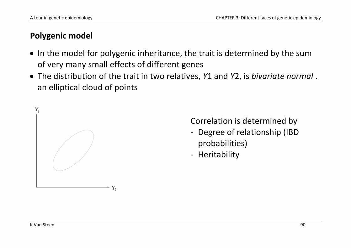
Polygenic model

In the model for polygenic inheritance, the trait is determined by the sum of very many small effects of different genes

The distribution of the trait in two relatives, Y1 and Y2, is bivariate normal . an elliptical cloud of points

Correlation is determined by - Degree of relationship (IBD

probabilities) - Heritability


K Van Steen 91

The Morton-Maclean model (the “mixed model”)

In this model, the trait is determined by additive effects of a single major locus plus a polygenic component. The bivariate distribution for two relatives is now a mixture of elliptical clouds:

The regressive model provides a convenient approximation to the “mixed

model” in genetics.


K Van Steen 92

The Morton-Maclean model (continued)

In this model it is necessary to allow for the manner in which pedigrees have been recruited into the study; Ascertained pedigrees in the study may be skewed, either deliberately or inadvertently, towards those with extreme trait values for one or more family members. This complicates the analyses even further…

Segregation analyses were often over-interpreted: the results depend on very strong model assumptions: - additivity of effects (major gene, polygenes, and environment) - bivariate normality of distribution of trait given genotype at the major

locus


K Van Steen 93

Types of variance component modeling

Variance components analysis can be undertaken with conventional techniques such as maximum likelihood or Markov chain Monte Carlo based approaches.

Genetic epidemiologists use various approaches to aid the specification of such models, including path analysis, which was invented by Sewall Wright nearly 100 years ago and the fitting is achieved by various programs.

Equivalent approaches can also be used for binary phenotypes (using

liability threshold models) and for traits that can best be expressed as a

survival time such as age at onset or age at death. (Burton et al, The Lancet, 2005)


K Van Steen 94

4.e The ideas of variance component modeling adjusted for binary traits

Aggregation of discrete traits, such as diseases in families have been studied by an extension of the Morton-Maclean model

Here a latent liability to disease is assumed that behaves as a quantitative trait, with a mixture of major gene and polygene effects. When liability exceeds a threshold, disease occurs

As in the quantitative trait case, this approach relies upon (too?) strong modeling assumptions


K Van Steen 95

4.f Quantifying the genetic importance in familial resemblance

Heritability

Recall: One of the principal reasons for fitting a variance components model

is to estimate the variance attributable to additive genetic effects

This quantity represents that component of the total phenotypic variance,

usually that can be attributed to unmeasured additive genetic effects. It

leads to the concept of narrow heritability.

In contrast, broad heritability is defined as the proportion of the total

phenotypic variance that is attributable to all genetic effects, including non-

additive effects at individual loci and between loci. (Burton et al, The Lancet, 2005)


K Van Steen 96

5 Linkage and Association

(Roche Genetics Education)


K Van Steen 97

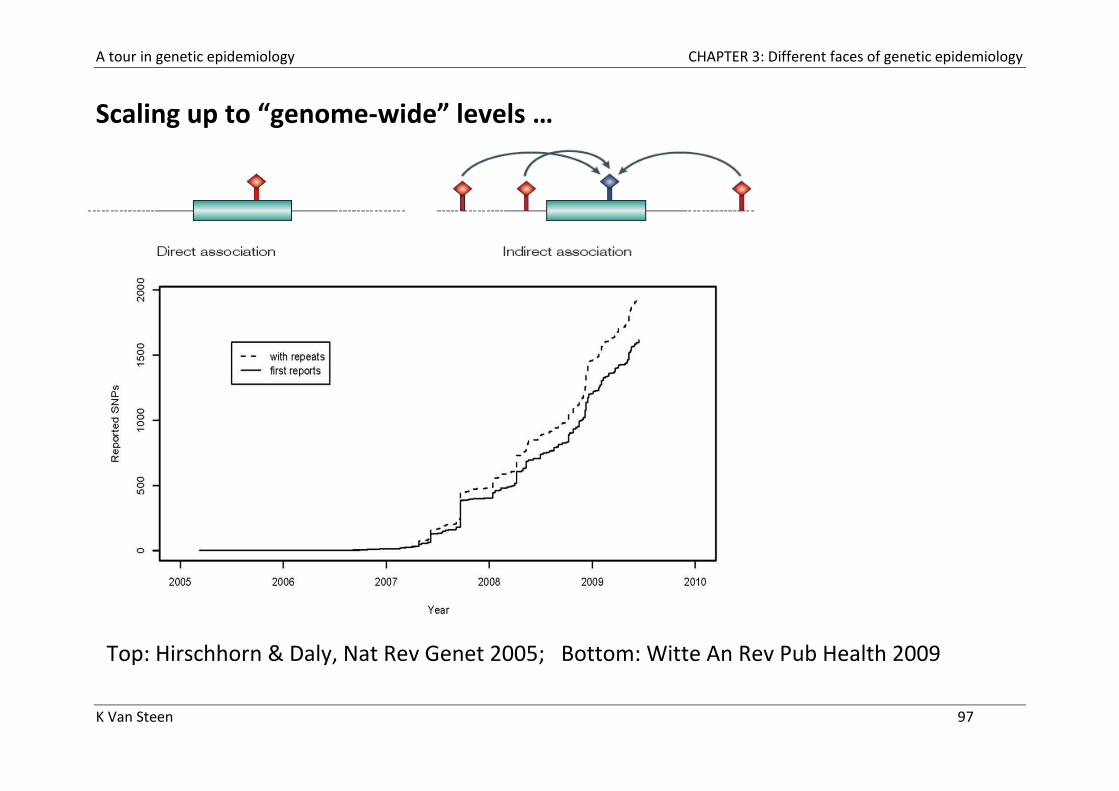
Scaling up to “genome-wide” levels …

Top: Hirschhorn & Daly, Nat Rev Genet 2005; Bottom: Witte An Rev Pub Health 2009


K Van Steen 98

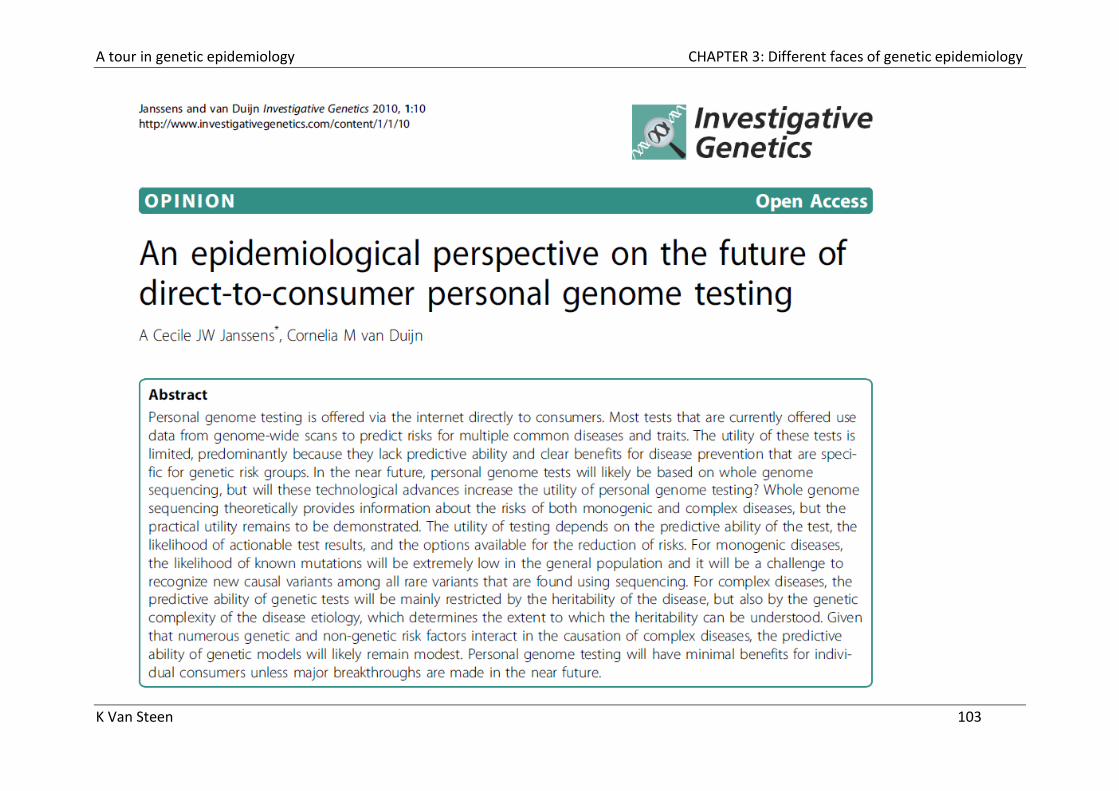
Genetic testing based on GWA studies

Multiple companies marketing direct to consumer genetic ‘test’ kits.

Send in spit.

Array technology (Illumina / Affymetrix).

Many results based on GWAS.

Companies:

- 23andMe

- deCODEme

- Navigenics


K Van Steen 99


K Van Steen 100

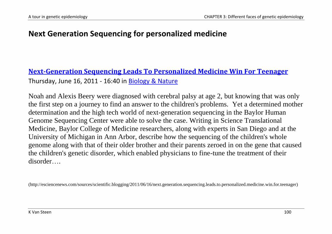
Next Generation Sequencing for personalized medicine

Next-Generation Sequencing Leads To Personalized Medicine Win For Teenager

Thursday, June 16, 2011 - 16:40 in Biology & Nature

Noah and Alexis Beery were diagnosed with cerebral palsy at age 2, but knowing that was only

the first step on a journey to find an answer to the children's problems. Yet a determined mother

determination and the high tech world of next-generation sequencing in the Baylor Human

Genome Sequencing Center were able to solve the case. Writing in Science Translational

Medicine, Baylor College of Medicine researchers, along with experts in San Diego and at the

University of Michigan in Ann Arbor, describe how the sequencing of the children's whole

genome along with that of their older brother and their parents zeroed in on the gene that caused

the children's genetic disorder, which enabled physicians to fine-tune the treatment of their

disorder….

(http://esciencenews.com/sources/scientific.blogging/2011/06/16/next.generation.sequencing.leads.to.personalized.medicine.win.for.teenager)

http://www.science20.com/news_articles/nextgeneration_sequencing_leads_personalized_medicine_win_teenager-80079

http://esciencenews.com/topics/biology.nature


K Van Steen 101

6 Genetic epidemiology and public health


K Van Steen 102


K Van Steen 103

INTRODUCTION TO GENETIC EPIDEMIOLOGY …...Introduction to Genetic Epidemiology CHAPTER 3: Different...

Documents

Transcript of INTRODUCTION TO GENETIC EPIDEMIOLOGY …...Introduction to Genetic Epidemiology CHAPTER 3: Different...