Introduction to General and Generalized Linear Modelshmad/GLM/Slides_2012/week13/lect13.pdf ·...

Introduction to General and Generalized Linear ModelsCourse Summary (plus integrated models)

Henrik MadsenJan Kloppenborg Møller

Anders Nielsen

May 5, 2012

Henrik Madsen Jan Kloppenborg Møller Anders Nielsen () Chapman & Hall May 5, 2012 1 / 40

This lecture

Course Summary

.....

Integrated models


What have we been doing?

Likelihood principle

General linear models

Generalized linear models

General mixed effects models

Repeated measurements

Random effects models

Hierarchical models

Crossed and nested models

Heteroscedasticity and correlation structures

Points on using R

The book covers a lot more than its title, and we went beyond that.


Likelihood inference

Likelihood function L(θ) = Pθ(Y = y)

Log likelihood function `(θ) = log(L(θ))

Score function `′(θ)

Maximum likelihood estimate θ = argmaxθ∈Θ

`(θ)

Observed information matrix −`′′(θ)Distribution of the ML estimator θ ∼ N(θ, (−`′′(θ))−1)

Likelihood ratio test 2(`A(θA,Y )− `B (θB ,Y )) ∼ χ2dim(A)−dim(B)

Invariance property

Dealing with nuisance parameters


Likelihood inference - When we use it

Indirectly all the time

Directly when no prepackaged tool is available


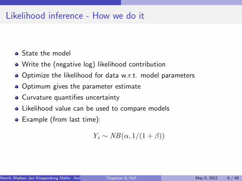
Likelihood inference - How we do it

State the model

Write the (negative log) likelihood contribution

Optimize the likelihood for data w.r.t. model parameters

Optimum gives the parameter estimate

Curvature quantifies uncertainty

Likelihood value can be used to compare models

Example (from last time):

Yi ∼ NB(α, 1/(1 + β))


General Linear Model

A general linear model is:

Y ∼ Nn(Xβ, σ2I )


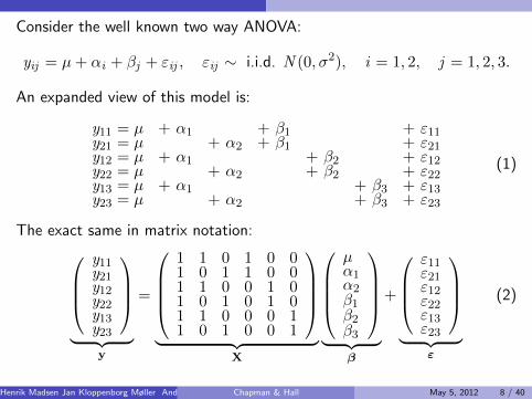
Consider the well known two way ANOVA:

yij = µ+ αi + βj + εij , εij ∼ i.i.d. N (0, σ2), i = 1, 2, j = 1, 2, 3.

An expanded view of this model is:

y11 = µ + α1 + β1 + ε11y21 = µ + α2 + β1 + ε21y12 = µ + α1 + β2 + ε12y22 = µ + α2 + β2 + ε22y13 = µ + α1 + β3 + ε13y23 = µ + α2 + β3 + ε23

(1)

The exact same in matrix notation:y11y21y12y22y13y23

︸︷︷︸

y

=

1 1 0 1 0 01 0 1 1 0 01 1 0 0 1 01 0 1 0 1 01 1 0 0 0 11 0 1 0 0 1

︸︷︷︸

X

µα1α2β1β2β3

︸︷︷︸

β

+

ε11ε21ε12ε22ε13ε23

︸︷︷︸

ε

(2)


y11y21y12y22y13y23

︸︷︷︸

y

=

1 1 0 1 0 01 0 1 1 0 01 1 0 0 1 01 0 1 0 1 01 1 0 0 0 11 0 1 0 0 1

︸︷︷︸

X

µα1α2β1β2β3

︸︷︷︸

β

+

ε11ε21ε12ε22ε13ε23

︸︷︷︸

ε

y is the vector of all observations

X is known as the design matrix

β is the vector of parameters

ε is a vector of independent N (0, σ2) “measurement noise”

The vector ε is said to follow a multivariate normal distributionMean vector 0Covariance matrix σ2IWritten as: ε ∼ N (0, σ2I)

y = Xβ + ε specifies the model, and everything can be calculatedfrom y and X.


General Linear Model - when we use it

When our observations are normally distributed

When a simple transformation (e.g. logarithm) can make ourobservations normally distributed

When our model prediction is a linear function of our modelparameters


General Linear Model - how we use it

Consider this dataset:

0 1000 2000 3000 4000

510

15

alt

y

F : PlaceboM : PlaceboF : TreatmentM : Treatment


Remember our talks about model formulation

How a statement like this

> fit0<-lm(y~sex*tmt+sex*tmt*alt)

Is really the model

yi = µ+α(Si)+β(Ti)+γ(Si ,Ti)+δ(Si)·ai+φ(Ti)·ai+ψ(Si ,Ti)·ai+εi

Which is over-parametrized, and really the same as:

yi = γ(Si ,Ti) + ψ(Si ,Ti) · ai + εi

But we use the long form to be able to test for model reductions


R example

> fit0<-lm(y~sex*tmt+sex*tmt*alt)

> drop1(fit0,test='F')

Single term deletions

Model:

y ~ sex * tmt + sex * tmt * alt

Df Sum of Sq RSS AIC F value Pr(F)

<none> 42.983 -68.437

sex:tmt:alt 1 0.077585 43.060 -70.257 0.1661 0.6846


> fit1<-lm(y~sex*tmt+(sex+tmt)*alt)



Model:

y ~ sex * tmt + (sex + tmt) * alt


<none> 43.060 -70.257

sex:tmt 1 0.245 43.305 -71.690 0.5287 0.4690

sex:alt 1 0.848 43.909 -70.306 1.8324 0.1791

tmt:alt 1 143.386 186.446 74.297 309.6786 <2e-16 ***

---

Signif. codes: 0 '***' 0.001 '**' 0.01 '*' 0.05 '.' 0.1 ' ' 1


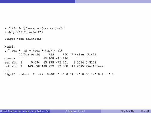
> fit2<-lm(y~sex+tmt+(sex+tmt)*alt)



Model:

y ~ sex + tmt + (sex + tmt) * alt


<none> 43.305 -71.690

sex:alt 1 0.694 43.999 -72.101 1.5054 0.2229

tmt:alt 1 143.628 186.933 72.558 311.7645 <2e-16 ***

---

Signif. codes: 0 '***' 0.001 '**' 0.01 '*' 0.05 '.' 0.1 ' ' 1


> fit3<-lm(y~sex+tmt*alt)

> fit4<-lm(y~sex+tmt:alt)



Model:

y ~ sex + tmt * alt


<none> 43.999 -72.101

sex 1 150.34 194.338 74.443 324.61 < 2.2e-16 ***

tmt:alt 1 143.95 187.946 71.099 310.80 < 2.2e-16 ***

---

Signif. codes: 0 '***' 0.001 '**' 0.01 '*' 0.05 '.' 0.1 ' ' 1

> anova(fit4,fit3)

Analysis of Variance Table

Model 1: y ~ sex + tmt:alt

Model 2: y ~ sex + tmt * alt

Res.Df RSS Df Sum of Sq F Pr(>F)

1 96 44.005

2 95 43.999 1 0.0061976 0.0134 0.9082


> fit4<-lm(y~sex+tmt:alt)



Model:

y ~ sex + tmt:alt


<none> 44.00 -74.087

sex 1 151.90 195.90 73.245 331.38 < 2.2e-16 ***

tmt:alt 2 950.58 994.59 233.716 1036.88 < 2.2e-16 ***

---

Signif. codes: 0 '***' 0.001 '**' 0.01 '*' 0.05 '.' 0.1 ' ' 1


Results

0 1000 2000 3000 4000

510

15

alt

y

F : PlaceboM : PlaceboF : TreatmentM : Treatment


Exponential families of distributions


Consider a univariate random variable Y with a distribution described by afamily of densities fY (y ; θ), θ ∈ Ω.

Definition (A natural exponential family)

A family of probability densities which can be written on the form

fY (y ; θ) = c(y) exp(θy − κ(θ)), θ ∈ Ω

is called a natural exponential family of distributions. The function κ(θ) iscalled the cumulant generator. This representation is called the canonicalparametrization of the family, and the parameter θ is called the canonicalparameter.




Definition (An exponential dispersion family)

A family of probability densities which can be written on the form

fY (y ; θ) = c(y , λ) exp(λθy − κ(θ))

is called an exponential dispersion family of distributions. The parameter λ > 0 iscalled the precision parameter.

Basic idea: separate the mean value related distributional propertiesdescribed by the cumulant generator κ(θ) from features as sample size,common variance, or common over-dispersion.

In some cases the precision parameter represents a known number ofobservations as for the binomial distribution, or a known shape parameter asfor the gamma (or χ2-) distribution.

In other cases the precision parameter represents an unknown dispersion likefor the normal distribution, or an over-dispersion that is not related to themean.



Example: Poisson distribution

Consider Y ∼ Pois(µ). The probability function for Y is:

fY (y ;µ) =µye−µ

y !

=1

y !expy log(µ)− µ

Comparing with the equation for the natural exponential family it is seenthat θ = log(µ) which means that µ = exp(θ).

Thus the Poisson distribution is a special case of a natural exponentialfamily with canonical parameter θ = log(µ), cumulant generatorκ(θ) = exp(θ) and c(y) = 1/y !.

The natural exponential family: fY (y ; θ) = c(y) exp(θy − κ(θ))


The Generalized Linear Model


Definition (The generalized linear model)

Assume that Y1,Y2, . . . ,Yn are mutually independent, and the densitycan be described by an exponential dispersion model with the samevariance function V (µ).A generalized linear model for Y1,Y2, . . . ,Yn describes an affinehypothesis for η1, η2, . . . , ηn , where

ηi = g(µi)

is a transformation of the mean values µ1, µ2, . . . , µn .The hypothesis is of the form

H0 : η − η0 ∈ L,

where L is a linear subspace Rn of dimension k , and where η0 denotes avector of known off-set values.



GLM vs GLM

General linear models Generalized linear models

Normal distribution Exponential dispersion family

Mean value linear Function of mean value linear

Independent observations Independent observations

Same variance Variance function of mean

Easy to apply Almost as easy to apply

Exact results Approximate results



Generalized Linear Model - when we use it

When observations are not following a normal distribution, but anexponential (dispersion) family

When a link function of then mean can be expressed as a linearfunction of the model parameters



Overdispersion

It may happen that even if one has tried to fit a rather comprehensivemodel (i.e. a model with many parameters), the fit is not satisfactory,and the residual deviance D

(y ;µ(β)

)is larger than what can be

explained by the χ2-distribution.

An explanation for such a poor model fit could be an improper choiceof linear predictor, or of link or response distribution.

If the residuals exhibit a random pattern, and there are no otherindications of misfit, then the explanation could be that the varianceis larger than indicated by V (µ).

We say that the data are overdispersed.



Overdispersion

When data are overdispersed, a more appropriate model might beobtained by including a dispersion parameter, σ2, in the model, i.e. adistribution model of the form with λi = wi/σ

2, and σ2 denoting theoverdispersion, Var[Yi ] = σ2V (µi)/wi .

As the dispersion parameter only would enter in the score function asa constant factor, this does not affect the estimation of the meanvalue parameters β.

However, because of the larger error variance, the distribution of thetest statistics will be influenced.

If, for some reasons, the parameter σ2 had been known beforehand,one would include this known value in the weights, wi .

Most often, when it is found necessary to choose a model withoverdispersion, σ2 shall be estimated from the data.



The mixed linear model

Consider now the one way ANOVA with random block effect:

Yij = µ+αi+Bj+εij , Bj ∼ N (0, σ2B ), εij ∼ N (0, σ2), i = 1, 2, j = 1, 2, 3

The matrix notation is:Y11Y21Y12Y22Y13Y23

︸︷︷︸

Y

=

1 1 01 0 11 1 01 0 11 1 01 0 1

︸︷︷︸

X

( µα1α2

)︸︷︷︸

β

+

1 0 01 0 00 1 00 1 00 0 10 0 1

︸︷︷︸

Z

(B1B2B3

)︸︷︷︸

U

+

ε11ε21ε12ε22ε13ε23

︸︷︷︸

ε

Notice how this matrix representation is constructed in exactly the sameway as for the fixed effects model — but separately for fixed and randomeffects.



A general linear mixed effects model

A general linear mixed model can be presented in matrix notation by:

Y = Xβ + ZU + ε, where U ∼ N (0,G) and ε ∼ N (0,R).

Y is the observation vector

X is the design matrix for the fixed effects

β is the vector containing the fixed effect parameters

Z is the design matrix for the random effectsU is the vector of random effects

It is assumed that U ∼ N (0,G)cov(Ui ,Uj ) = Gi,j (typically G has a very simple structure (forinstance diagonal))

ε is the vector of residual errorsIt is assumed that ε ∼ N (0,R)cov(εi , εj ) = Ri,j (typically R is diagonal, but we shall later see someuseful exceptions for repeated measurements)



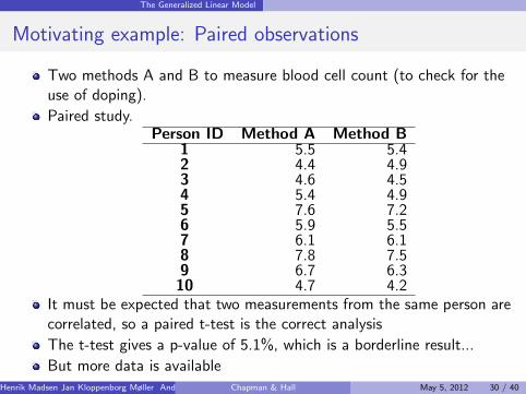
Motivating example: Paired observations

Two methods A and B to measure blood cell count (to check for theuse of doping).

Paired study.Person ID Method A Method B

1 5.5 5.42 4.4 4.93 4.6 4.54 5.4 4.95 7.6 7.26 5.9 5.57 6.1 6.18 7.8 7.59 6.7 6.310 4.7 4.2

It must be expected that two measurements from the same person arecorrelated, so a paired t-test is the correct analysis

The t-test gives a p-value of 5.1%, which is a borderline result...

But more data is availableHenrik Madsen Jan Kloppenborg Møller Anders Nielsen () Chapman & Hall May 5, 2012 30 / 40


In addition to the planned study 10 persons were measured with onlyone method

Want to use all data, which is possiblewith random effects

Assume these 20 are ramdomly selectedfrom a population where the blod cellcount is normally distributed

Consider the following model:Ci = α(Mi) + B(Pi) + εi , i = 1 . . . 30α(Mi) the 2 fixed method effectsB(Pi) ∼ N (0, σ2

P ) the 20 rand. eff.εi ∼ N (0, σ2

R) measurement noiseAll B(Pi) and εi are independent

This model uses all data

Allows us to test method difference

ID Meth. A Meth. B1 5.5 5.42 4.4 4.93 4.6 4.54 5.4 4.95 7.6 7.26 5.9 5.57 6.1 6.18 7.8 7.59 6.7 6.310 4.7 4.211 3.412 4.713 3.914 2.515 4.116 4.017 6.318 6.019 6.420 3.5



General Linear Mixed Model - when we use it

When our observations are normally distributed

When a simple transformation (e.g. logarithm) can make ourobservations normally distributed

When our model prediction is a linear function of our modelparameters

When observational units are themselves sampled from a largerpopulation (where normal assumption is OK)

When it is helpful in expressing a needed covariance structure

When we have repeated measurements



General (non-linear and/or non-normal) Mixed Models

The general mixed effects model can be represented by its likelihoodfunction:

LM (θ;y) =

∫Rq

L(θ;u ,y)du

– y is the observed random variables

– u is the q unobserved random variables

– θ is the model parameters to be estimated

The likelihood function L is the joint likelihood of both the observed andthe unobserved random variables.

The likelihood function for estimating θ is the marginal likelihood LM

obtained by integrating out the unobserved random variables.



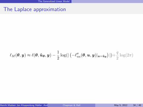
The Laplace approximation

`M (θ,y) ≈ `(θ, uθ,y)− 1

2log(|

(−`′′uu(θ,u ,y)|u=uθ

)|)+q

2log(2π)



Formulation of hierarchical model

Theorem (Compound Poisson Gamma model)

Consider a hierarchical model for Y specified by

Y |µ ∼ Pois(µ),

µ ∼ G(α, β),

i.e. a two stage model.

In the first stage a random mean value µ is selected according to a Gammadistribution. The Y is generated according to a Poisson distribution withthat value as mean value. Then the the marginal distribution of Y is anegative binomial distribution, Y ∼ NB(α, 1/(1 + β))



Hierarchical Binomial-Beta distribution model

The natural conjugate distribution to the binomial is a Beta-distribution.

Theorem

Consider the generalized one-way random effects model for Z1,Z2, . . . ,Zk givenby

Zi |pi ∼ B(n, pi)

pi ∼ Beta(α, β)

i.e. the conditional distribution of Zi given pi is a Binomial distribution, and thedistribution of the mean value pi is a Beta distribution. Then the marginaldistribution of Zi is a Polya distributionwith probability function

P [Z = z ] = gZ (z ) =

(n

z

)Γ(α+ x )

Γ(α)

Γ(β + n − z )

Γ(β)

Γ(α+ β)

Γ(α+ β + n)

for z = 0, 1, 2, . . . ,n.



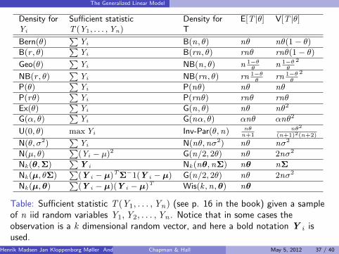
Density for Sufficient statistic Density for E[T |θ] V[T |θ]Yi T (Y1, . . . ,Yn) T

Bern(θ)∑

Yi B(n, θ) nθ nθ(1− θ)B(r , θ)

∑Yi B(rn, θ) rnθ rnθ(1− θ)

Geo(θ)∑

Yi NB(n, θ) n 1−θθ

n 1−θθ

2

NB(r , θ)∑

Yi NB(rn, θ) rn 1−θθ

rn 1−θθ

2

P(θ)∑

Yi P(nθ) nθ nθ

P(rθ)∑

Yi P(rnθ) rnθ rnθ

Ex(θ)∑

Yi G(n, θ) nθ nθ2

G(α, θ)∑

Yi G(nα, θ) αnθ αnθ2

U(0, θ) maxYi Inv-Par(θ,n) nθn+1

nθ2

(n+1)2(n+2)

N(θ, σ2)∑

Yi N(nθ,nσ2) nθ nσ2

N(µ, θ)∑

(Yi − µ)2 G(n/2, 2θ) nθ 2nσ2

Nk (θ,Σ)∑

Y i Nk (nθ,nΣ) nθ nΣ

Nk (µ, θΣ)∑

(Y i − µ)TΣ−1(Y i − µ) G(n/2, 2θ) nθ 2nσ2

Nk (µ,θ)∑

(Y i − µ)(Y i − µ)T Wis(k ,n,θ) nθ

Table: Sufficient statistic T (Y1, . . . ,Yn) (see p. 16 in the book) given a sampleof n iid random variables Y1,Y2, . . . ,Yn . Notice that in some cases theobservation is a k dimensional random vector, and here a bold notation Y i isused.



Conditional density Conjugate prior Posterior density for Marginal density ofof T given θ for θ θ after the T = t(Y1, . . . ,Yn)

obs. T = t(y1, . . . , yn)

B(n, θ) Beta(α, β) Beta(t + α,n + β − t) Pl(n, α, α+ β)

NB(n, θ) Beta(α, β) Beta(n + α, β + t) NPl(n, β, α+ β)

P(nθ) G(α, 1/β) G(t + α, 1/(β + n) NB(α, β/(β + n))

G(n, θ) Inv-G(α, β) Inv-G(n + α, β + t) Inv-Beta(α,n, β)

Inv-Par(θ,n) Par(β, µ) Par(max(t , β),n + µ) BParβ, µ,n)

N(nθ,nσ2) N(µ, σ20) N(µ1, σ

21) N(nµ,nσ2 + n2σ2

0)µ1 = (µ/σ2

0 + t/σ2)1/σ2

1 = 1/σ20 + n/σ2

Nk (nθ,nΣ) Nk (µ,Σ0) Nk (µ1,Σ1) Nk (nµ,nΣ+Σ0)µ1 = Σ1(Σ

−10 µ+Σ−1t)

Σ−11 = Σ−1

0 + nΣ−1

Table: Conditional densities of the statistic T given the parameter θ, conjugateprior densities for θ, posterior densities for θ after having observed the statisticT = t(y1, . . . , yn), and the marginal densities for T = t(Y1, . . . ,Yn) – cf. alsothe discussion on page 16 and 17 in the book.(Notice that in some cases theobservation is a random vector)



What else is out there

Time series

Multivariate analysis

Non-parametric models

Integrated analysis

...

But you are now well prepared to tackle those also.



Integrated analysis

One nice thing about being able to write your own likelihood isflexibility

Remember how we set up the log likelihood as the sum of thecontributions from each independent observation:

`(θ,X ) = `(θ, x1) + `(θ, x2) + · · ·+ `(θ, xn)

We did not say that our observations should come from the samedistribution

It is no problem to have some that are say normally distributed andothers that are Poisson distributed inform us about the same modelparameters

That is only problematic when we are confined to a formula interface.


Introduction to General and Generalized Linear Modelshmad/GLM/Slides_2012/week13/lect13.pdf ·...

Documents

Transcript of Introduction to General and Generalized Linear Modelshmad/GLM/Slides_2012/week13/lect13.pdf ·...