INTRODUCTION TO FUNCTIONAL ANALYSISkisilv/courses/math3263m.pdf · 2 VLADIMIR V. KISIL 4. Fourier...
147
This work is licensed under a Creative Commons “Attribution-NonCommercial-ShareAlike 4.0 Interna- tional” licence. INTRODUCTION TO FUNCTIONAL ANALYSIS VLADIMIR V. KISIL ABSTRACT. This is lecture notes for several courses on Functional Analysis at School of Mathematics of University of Leeds. They are based on the notes of Dr. Matt Daws, Prof. Jonathan R. Partington and Dr. David Salinger used in the previous years. Some sections are borrowed from the textbooks, which I used since being a student myself. However all misprints, omissions, and errors are only my responsibility. I am very grateful to Filipa Soares de Almeida, Eric Borgnet, Pasc Gavruta for pointing out some of them. Please let me know if you find more. The notes are available also for download in PDF. The suggested textbooks are [1, 6, 8, 9]. The other nice books with many interest- ing problems are [3, 7]. Exercises with stars are not a part of mandatory material but are nevertheless worth to hear about. And they are not necessarily difficult, try to solve them! CONTENTS List of Figures 3 Notations and Assumptions 4 Integrability conditions 4 1. Motivating Example: Fourier Series 4 1.1. Fourier series: basic notions 4 1.2. The vibrating string 8 1.3. Historic: Joseph Fourier 10 2. Basics of Linear Spaces 11 2.1. Banach spaces (basic definitions only) 12 2.2. Hilbert spaces 14 2.3. Subspaces 17 2.4. Linear spans 20 3. Orthogonality 21 3.1. Orthogonal System in Hilbert Space 22 3.2. Bessel’s inequality 23 3.3. The Riesz–Fischer theorem 26 3.4. Construction of Orthonormal Sequences 27 3.5. Orthogonal complements 29 Date: 20th February 2018. 1
Transcript of INTRODUCTION TO FUNCTIONAL ANALYSISkisilv/courses/math3263m.pdf · 2 VLADIMIR V. KISIL 4. Fourier...
This work is licensed under a Creative Commons“Attribution-NonCommercial-ShareAlike 4.0 Interna-tional” licence.
INTRODUCTION TO FUNCTIONAL ANALYSIS
VLADIMIR V. KISIL
ABSTRACT. This is lecture notes for several courses on Functional Analysis atSchool of Mathematics of University of Leeds. They are based on the notes ofDr. Matt Daws, Prof. Jonathan R. Partington and Dr. David Salinger used in theprevious years. Some sections are borrowed from the textbooks, which I used sincebeing a student myself. However all misprints, omissions, and errors are only myresponsibility. I am very grateful to Filipa Soares de Almeida, Eric Borgnet, PascGavruta for pointing out some of them. Please let me know if you find more.
The notes are available also for download in PDF.The suggested textbooks are [1,6,8,9]. The other nice books with many interest-
ing problems are [3, 7].Exercises with stars are not a part of mandatory material but are nevertheless
worth to hear about. And they are not necessarily difficult, try to solve them!
CONTENTS
List of Figures 3Notations and Assumptions 4Integrability conditions 41. Motivating Example: Fourier Series 41.1. Fourier series: basic notions 41.2. The vibrating string 81.3. Historic: Joseph Fourier 102. Basics of Linear Spaces 112.1. Banach spaces (basic definitions only) 122.2. Hilbert spaces 142.3. Subspaces 172.4. Linear spans 203. Orthogonality 213.1. Orthogonal System in Hilbert Space 223.2. Bessel’s inequality 233.3. The Riesz–Fischer theorem 263.4. Construction of Orthonormal Sequences 273.5. Orthogonal complements 29
Date: 20th February 2018.
1

2 VLADIMIR V. KISIL
4. Fourier Analysis 304.1. Fourier series 314.2. Fejer’s theorem 324.3. Parseval’s formula 374.4. Some Application of Fourier Series 385. Duality of Linear Spaces 435.1. Dual space of a normed space 445.2. Self-duality of Hilbert space 466. Operators 466.1. Linear operators 466.2. B(H) as a Banach space (and even algebra) 476.3. Adjoints 496.4. Hermitian, unitary and normal operators 497. Spectral Theory 527.1. The spectrum of an operator on a Hilbert space 527.2. The spectral radius formula 547.3. Spectrum of Special Operators 558. Compactness 568.1. Compact operators 568.2. Hilbert–Schmidt operators 609. The spectral theorem for compact normal operators 629.1. Spectrum of normal operators 629.2. Compact normal operators 6410. Applications to integral equations 6611. Banach and Normed Spaces 7211.1. Normed spaces 7211.2. Bounded linear operators 7611.3. Dual Spaces 7611.4. Hahn–Banach Theorem 7811.5. C(X) Spaces 8012. Measure Theory 8012.1. Basic Measure Theory 8112.2. Extension of Measures 8312.3. Complex-Valued Measures and Charges 8712.4. Constructing Measures, Products 8913. Integration 9013.1. Measurable functions 9013.2. Lebsgue Integral 9213.3. Properties of the Lebesgue Integral 9613.4. Integration on Product Measures 10013.5. Absolute Continuity of Measures 10314. Functional Spaces 104

INTRODUCTION TO FUNCTIONAL ANALYSIS 3
14.1. Integrable Functions 10414.2. Dense Subspaces in Lp 10814.3. Continuous functions 11014.4. Riesz Representation Theorem 11315. Fourier Transform 11615.1. Convolutions on Commutative Groups 11615.2. Characters of Commutative Groups 11915.3. Fourier Transform on Commutative Groups 12115.4. Fourier Integral 122Appendix A. Tutorial Problems 126A.1. Tutorial problems I 126A.2. Tutorial problems II 127A.3. Tutorial Problems III 127A.4. Tutorial Problems IV 128A.5. Tutorial Problems V 129A.6. Tutorial Problems VI 130A.7. Tutorial Problems VII 131Appendix B. Solutions of Tutorial Problems 133Appendix C. Course in the Nutshell 134C.1. Some useful results and formulae (1) 134C.2. Some useful results and formulae (2) 135Appendix D. Supplementary Sections 138D.1. Reminder from Complex Analysis 138References 138Index 140
LIST OF FIGURES
1 Triangle inequality 122 Different unit balls 143 To the parallelogram identity. 164 Jump function as a limit of continuous functions 185 The Pythagoras’ theorem 226 Best approximation from a subspace 247 Best approximation by three trigonometric polynomials 258 Legendre and Chebyshev polynomials 289 A modification of continuous function to periodic 3110 The Fejer kernel 3411 The dynamics of a heat equation 4012 Appearance of dissonance 41

4 VLADIMIR V. KISIL
13 Different musical instruments 4214 Fourier series for different musical instruments 4315 Two frequencies separated in time 4416 Distance between scales of orthonormal vectors 5817 The ε/3 argument to estimate |f(x) − f(y)|. 59
NOTATIONS AND ASSUMPTIONS
Z+, R+ denotes non-negative integers and reals.x,y, z, . . . denotes vectors.λ,µ,ν, . . . denotes scalars.<z, =z stand for real and imaginary parts of a complex number z.
Integrability conditions. In this course, the functions we consider will be real orcomplex valued functions defined on the real line which are locally Riemann integ-rable. This means that they are Riemann integrable on any finite closed interval[a,b]. (A complex valued function is Riemann integrable iff its real and imagin-ary parts are Riemann-integrable.) In practice, we shall be dealing mainly withbounded functions that have only a finite number of points of discontinuity in anyfinite interval. We can relax the boundedness condition to allow improper Riemannintegrals, but we then require the integral of the absolute value of the function toconverge.
We mention this right at the start to get it out of the way. There are many fascin-ating subtleties connected with Fourier analysis, but those connected with technicalaspects of integration theory are beyond the scope of the course. It turns out thatone needs a “better” integral than the Riemann integral: the Lebesgue integral, andI commend the module, Linear Analysis 1, which includes an introduction to thattopic which is available to MM students (or you could look it up in Real and Com-plex Analysis by Walter Rudin). Once one has the Lebesgue integral, one can startthinking about the different classes of functions to which Fourier analysis applies:the modern theory (not available to Fourier himself) can even go beyond functionsand deal with generalized functions (distributions) such as the Dirac delta functionwhich may be familiar to some of you from quantum theory.
From now on, when we say “function”, we shall assume the conditions of thefirst paragraph, unless anything is stated to the contrary.
1. MOTIVATING EXAMPLE: FOURIER SERIES
1.1. Fourier series: basic notions. Before proceed with an abstract theory we con-sider a motivating example: Fourier series.

INTRODUCTION TO FUNCTIONAL ANALYSIS 5
1.1.1. 2π-periodic functions. In this part of the course we deal with functions (asabove) that are periodic.
We say a function f : R → C is periodic with period T > 0 if f(x + T) = f(x) forall x ∈ R. For example, sin x, cos x, eix(= cos x + i sin x) are periodic with period2π. For k ∈ R \ 0, sinkx, coskx, and eikx are periodic with period 2π/|k|. Constantfunctions are periodic with period T , for any T > 0. We shall specialize to periodicfunctions with period 2π: we call them 2π-periodic functions, for short. Note thatcosnx, sinnx and einx are 2π-periodic for n ∈ Z. (Of course these are also 2π/|n|-periodic.)
Any half-open interval of length T is a fundamental domain of a periodic function fof period T . Once you know the values of f on the fundamental domain, you knowthem everywhere, because any point x in R can be written uniquely as x = w+ nTwhere n ∈ Z andw is in the fundamental domain. Thus f(x) = f(w+(n−1)T+T) =· · · = f(w+ T) = f(w).
For 2π-periodic functions, we shall usually take the fundamental domain to be] − π,π]. By abuse of language, we shall sometimes refer to [−π,π] as the funda-mental domain. We then have to be aware that f(π) = f(−π).
1.1.2. Integrating the complex exponential function. We shall need to calculate∫baeikx dx,
for k ∈ R. Note first that when k = 0, the integrand is the constant function 1, so theresult is b−a. For non-zero k,
∫baeikx dx =
∫ba(coskx+ i sinkx)dx = (1/k)[(sinkx−
i coskx)]ba = (1/ik)[(cos kx+ i sinkx)]ba = (1/ik)[eikx]ba = (1/ik)(eikb − eika). Notethat this is exactly the result you would have got by treating i as a real constantand using the usual formula for integrating eax. Note also that the cases k = 0 andk 6= 0 have to be treated separately: this is typical.
Definition 1.1. Let f : R → C be a 2π-periodic function which is Riemann integ-rable on [−π,π]. For each n ∈ Z we define the Fourier coefficient f(n) by
f(n) =1
2π
π∫−π
f(x)e−inx dx .
Remark 1.2. (i) f(n) is a complex number whose modulus is the amplitudeand whose argument is the phase (of that component of the original func-tion).
(ii) If f and g are Riemann integrable on an interval, then so is their product,so the integral is well-defined.
(iii) The constant before the integral is to divide by the length of the interval.(iv) We could replace the range of integration by any interval of length 2π,
without altering the result, since the integrand is 2π-periodic.(v) Note the minus sign in the exponent of the exponential. The reason for this
will soon become clear.

6 VLADIMIR V. KISIL
Example 1.3. (i) f(x) = c then f(0) = c and f(n) = 0 when n 6= 0.(ii) f(x) = eikx, where k is an integer. f(n) = δnk.
(iii) f is 2π periodic and f(x) = x on ] − π,π]. (Diagram) Then f(0) = 0 and, forn 6= 0,
f(n) =1
2π
π∫−π
xe−inx dx=
[−xe−inx
2πin
]π−π
+1
in
1
2π
π∫−π
einx dx=(−1)ni
n.
Proposition 1.4 (Linearity). If f and g are 2π-periodic functions and c and d are complexconstants, then, for all n ∈ Z,
(cf+ dg) (n) = cf(n) + dg(n) .
Corollary 1.5. If p(x) =∑k
−k cneinx, then p(n) = cn for |n| 6 k and = 0, for |n| > k.
p(x) =∑n∈Z
p(n)einx .
This follows immediately from Ex. 1.3(ii) and Prop.1.4.
Remark 1.6. (i) This corollary explains why the minus sign is natural in thedefinition of the Fourier coefficients.
(ii) The first part of the course will be devoted to the question of how far thisresult can be extended to other 2π-periodic functions, that is, for whichfunctions, and for which interpretations of infinite sums is it true that
(1.1) f(x) =∑n∈Z
f(n)einx .
Definition 1.7.∑n∈Z f(n)e
inx is called the Fourier series of the 2π-periodic functionf.
For real-valued functions, the introduction of complex exponentials seems arti-ficial: indeed they can be avoided as follows. We work with (1.1) in the case of afinite sum: then we can rearrange the sum as
f(0) +∑n>0
(f(n)einx + f(−n)e−inx)
= f(0) +∑n>0
[(f(n) + f(−n)) cosnx+ i(f(n) − f(−n)) sinnx]
=a0
2+∑n>0
(an cosnx+ bn sinnx)

INTRODUCTION TO FUNCTIONAL ANALYSIS 7
Here
an = (f(n) + f(−n)) =1
2π
π∫−π
f(x)(e−inx + einx)dx
=1
π
π∫−π
f(x) cosnxdx
for n > 0 and
bn = i((f(n) − f(−n)) =1
π
π∫−π
f(x) sinnxdx
for n > 0. a0 = 1π
π∫−π
f(x)dx, the constant chosen for consistency.
The an and bn are also called Fourier coefficients: if it is necessary to distinguishthem, we may call them Fourier cosine and sine coefficients, respectively.
We note that if f is real-valued, then the an and bn are real numbers and so<f(n) = <f(−n), =f(n) = −=f(n): thus f(−n) is the complex conjugate of f(n).Further, if f is an even function then all the sine coefficients are 0 and if f is an oddfunction, all the cosine coefficients are zero. We note further that the sine and cosinecoefficients of the functions coskx and sinkx themselves have a particularly simpleform: ak = 1 in the first case and bk = 1 in the second. All the rest are zero.
For example, we should expect the 2π-periodic function whose value on ] −π,π]
is x to have just sine coefficients: indeed this is the case: an = 0 and bn = i(f(n) −
f(−n)) = (−1)n+12/n for n > 0.The above question can then be reformulated as “to what extent is f(x) represen-
ted by the Fourier series a0/2 +∑n>0(an cos x+ bn sin x)?” For instance how well
does∑
(−1)n+1(2/n) sinnx represent the 2π-periodic sawtooth function f whosevalue on ] − π,π] is given by f(x) = x. The easy points are x = 0, x = π, where theterms are identically zero. This gives the ‘wrong’ value for x = π, but, if we look atthe periodic function near π, we see that it jumps from π to −π, so perhaps the meanof those values isn’t a bad value for the series to converge to. We could concludethat we had defined the function incorrectly to begin with and that its value at thepoints (2n + 1)π should have been zero anyway. In fact one can show (ref. ) thatthe Fourier series converges at all other points to the given values of f, but I shan’tinclude the proof in this course. The convergence is not at all uniform (it can’t be,because the partial sums are continuous functions, but the limit is discontinuous.)In particular we get the expansion
π
2= 2(1 − 1/3 + 1/5 − · · · )
which can also be deduced from the Taylor series for tan−1.

8 VLADIMIR V. KISIL
1.2. The vibrating string. In this subsection we shall discuss the formal solutionsof the wave equation in a special case which Fourier dealt with in his work.
We discuss the wave equation
(1.2)∂2y
∂x2=
1
K2
∂2y
∂t2,
subject to the boundary conditions
(1.3) y(0, t) = y(π, t) = 0,
for all t > 0, and the initial conditions
y(x, 0) = F(x),
yt(x, 0) = 0.
This is a mathematical model of a string on a musical instrument (guitar, harp,violin) which is of length π and is plucked, i.e. held in the shape F(x) and released attime t = 0. The constant K depends on the length, density and tension of the string.We shall derive the formal solution (that is, a solution which assumes existence andignores questions of convergence or of domain of definition).
1.2.1. Separation of variables. We first look (as Fourier and others before him did) forsolutions of the form y(x, t) = f(x)g(t). Feeding this into the wave equation (1.2)we get
f′′(x)g(t) =1
K2f(x)g′′(t)
and so, dividing by f(x)g(t), we have
(1.4)f′′(x)
f(x)=
1
K2
g′′(t)
g(t).
The left-hand side is an expression in x alone, the right-hand side in t alone. Theconclusion must be that they are both identically equal to the same constant C, say.
We have f′′(x) − Cf(x) = 0 subject to the condition f(0) = f(π) = 0. Workingthrough the method of solving linear second order differential equations tells youthat the only solutions occur when C = −n2 for some positive integer n and thecorresponding solutions, up to constant multiples, are f(x) = sinnx.
Returning to equation (1.4) gives the equation g′′(t)+K2n2g(t) = 0 which has thegeneral solution g(t) = an cosKnt + bn sinKnt. Thus the solution we get throughseparation of variables, using the boundary conditions but ignoring the initial con-ditions, are
yn(x, t) = sinnx(an cosKnt+ bn sinKnt) ,
for n > 1.

INTRODUCTION TO FUNCTIONAL ANALYSIS 9
1.2.2. Principle of Superposition. To get the general solution we just add together allthe solutions we have got so far, thus
(1.5) y(x, t) =
∞∑n=1
sinnx(an cosKnt+ bn sinKnt)
ignoring questions of convergence. (We can do this for a finite sum without dif-ficulty because we are dealing with a linear differential equation: the iffy bit is toextend to an infinite sum.)
We now apply the initial condition y(x, 0) = F(x) (note F has F(0) = F(π) = 0).This gives
F(x) =
∞∑n=1
an sinnx .
We apply the reflection trick: the right-hand side is a series of odd functions so ifwe extend F to a function G by reflection in the origin, giving
G(x) :=
F(x) , if 0 6 x 6 π;−F(−x) , if − π < x < 0.
we have
G(x) =
∞∑n=1
an sinnx ,
for −π 6 x 6 π.If we multiply through by sin rx and integrate term by term, we get
ar =1
π
π∫−π
G(x) sin rx dx
so, assuming that this operation is valid, we find that the an are precisely the sinecoefficients of G. (Those of you who took Real Analysis 2 last year may rememberthat a sufficient condition for integrating term-by -term is that the series which isintegrated is itself uniformly convergent.)
If we now assume, further, that the right-hand side of (1.5) is differentiable (termby term) we differentiate with respect to t, and set t = 0, to get
(1.6) 0 = yt(x, 0) =
∞∑n=1
bnKn sinnx.
This equation is solved by the choice bn = 0 for all n, so we have the followingresult
Proposition 1.8 (Formal). Assuming that the formal manipulations are valid, a solutionof the differential equation (1.2) with the given boundary and initial conditions is
(2.11) y(x, t) =
∞∑1
an sinnx cosKnt ,
10 VLADIMIR V. KISIL
where the coefficients an are the Fourier sine coefficients
an =1
π
π∫−π
G(x) sinnxdx
of the 2π periodic function G, defined on ] − π,π] by reflecting the graph of F in the origin.
Remark 1.9. This leaves us with the questions(i) For which F are the manipulations valid?
(ii) Is this the only solution of the differential equation? (which I’m not goingto try to answer.)
(iii) Is bn = 0 all n the only solution of (1.6)? This is a special case of theuniqueness problem for trigonometric series.
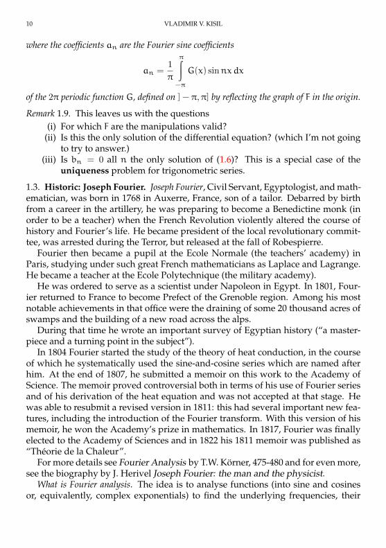
1.3. Historic: Joseph Fourier. Joseph Fourier, Civil Servant, Egyptologist, and math-ematician, was born in 1768 in Auxerre, France, son of a tailor. Debarred by birthfrom a career in the artillery, he was preparing to become a Benedictine monk (inorder to be a teacher) when the French Revolution violently altered the course ofhistory and Fourier’s life. He became president of the local revolutionary commit-tee, was arrested during the Terror, but released at the fall of Robespierre.
Fourier then became a pupil at the Ecole Normale (the teachers’ academy) inParis, studying under such great French mathematicians as Laplace and Lagrange.He became a teacher at the Ecole Polytechnique (the military academy).
He was ordered to serve as a scientist under Napoleon in Egypt. In 1801, Four-ier returned to France to become Prefect of the Grenoble region. Among his mostnotable achievements in that office were the draining of some 20 thousand acres ofswamps and the building of a new road across the alps.
During that time he wrote an important survey of Egyptian history (“a master-piece and a turning point in the subject”).
In 1804 Fourier started the study of the theory of heat conduction, in the courseof which he systematically used the sine-and-cosine series which are named afterhim. At the end of 1807, he submitted a memoir on this work to the Academy ofScience. The memoir proved controversial both in terms of his use of Fourier seriesand of his derivation of the heat equation and was not accepted at that stage. Hewas able to resubmit a revised version in 1811: this had several important new fea-tures, including the introduction of the Fourier transform. With this version of hismemoir, he won the Academy’s prize in mathematics. In 1817, Fourier was finallyelected to the Academy of Sciences and in 1822 his 1811 memoir was published as“Theorie de la Chaleur”.
For more details see Fourier Analysis by T.W. Korner, 475-480 and for even more,see the biography by J. Herivel Joseph Fourier: the man and the physicist.
What is Fourier analysis. The idea is to analyse functions (into sine and cosinesor, equivalently, complex exponentials) to find the underlying frequencies, their

INTRODUCTION TO FUNCTIONAL ANALYSIS 11
strengths (and phases) and, where possible, to see if they can be recombined (syn-thesis) into the original function. The answers will depend on the original prop-erties of the functions, which often come from physics (heat, electronic or soundwaves). This course will give basically a mathematical treatment and so will beinterested in mathematical classes of functions (continuity, differentiability proper-ties).
2. BASICS OF LINEAR SPACES
A person is solely the concentration of an infinite set of interre-lations with another and others, and to separate a person fromthese relations means to take away any real meaning of thelife.
Vl. Soloviev
A space around us could be described as a three dimensional Euclidean space.To single out a point of that space we need a fixed frame of references and three realnumbers, which are coordinates of the point. Similarly to describe a pair of pointsfrom our space we could use six coordinates; for three points—nine, end so on.This makes it reasonable to consider Euclidean (linear) spaces of an arbitrary finitedimension, which are studied in the courses of linear algebra.
The basic properties of Euclidean spaces are determined by its linear and metricstructures. The linear space (or vector space) structure allows to add and subtract vec-tors associated to points as well as to multiply vectors by real or complex numbers(scalars).
The metric space structure assign a distance—non-negative real number—to a pairof points or, equivalently, defines a length of a vector defined by that pair. A metric(or, more generally a topology) is essential for definition of the core analytical no-tions like limit or continuity. The importance of linear and metric (topological)structure in analysis sometime encoded in the formula:
(2.1) Analysis = Algebra + Geometry .
On the other hand we could observe that many sets admit a sort of linear andmetric structures which are linked each other. Just few among many other ex-amples are:
• The set of convergent sequences;• The set of continuous functions on [0, 1].
It is a very mathematical way of thinking to declare such sets to be spaces and call theirelements points.
But shall we lose all information on a particular element (e.g. a sequence 1/n)if we represent it by a shapeless and size-less “point” without any inner config-uration? Surprisingly not: all properties of an element could be now retrieved notfrom its inner configuration but from interactions with other elements through linearand metric structures. Such a “sociological” approach to all kind of mathematicalobjects was codified in the abstract category theory.
12 VLADIMIR V. KISIL
Another surprise is that starting from our three dimensional Euclidean space andwalking far away by a road of abstraction to infinite dimensional Hilbert spaces weare arriving just to yet another picture of the surrounding space—that time on thelanguage of quantum mechanics.
The distance from Manchester to Liverpool is 35 miles—justabout the mileage in the opposite direction!
A tourist guide to England
2.1. Banach spaces (basic definitions only). The following definition generalisesthe notion of distance known from the everyday life.
Definition 2.1. A metric (or distance function) d on a setM is a function d :M×M→R+ from the set of pairs to non-negative real numbers such that:
(i) d(x,y) > 0 for all x, y ∈M, d(x,y) = 0 implies x = y .(ii) d(x,y) = d(y, x) for all x and y inM.
(iii) d(x,y) + d(y, z) > d(x, z) for all x, y, and z inM (triangle inequality).
Exercise 2.2. Let M be the set of UK’s cities are the following function are metricsonM:
(i) d(A,B) is the price of 2nd class railway ticket from A to B.(ii) d(A,B) is the off-peak driving time from A to B.
The following notion is a useful specialisation of metric adopted to the linearstructure.
Definition 2.3. Let V be a (real or complex) vector space. A norm on V is a real-valued function, written ‖x‖, such that
(i) ‖x‖ > 0 for all x ∈ V , and ‖x‖ = 0 implies x = 0.(ii) ‖λx‖ = |λ| ‖x‖ for all scalar λ and vector x.
(iii) ‖x+ y‖ 6 ‖x‖+ ‖y‖ (triangle inequality).A vector space with a norm is called a normed space.
The connection between norm and metric is as follows:
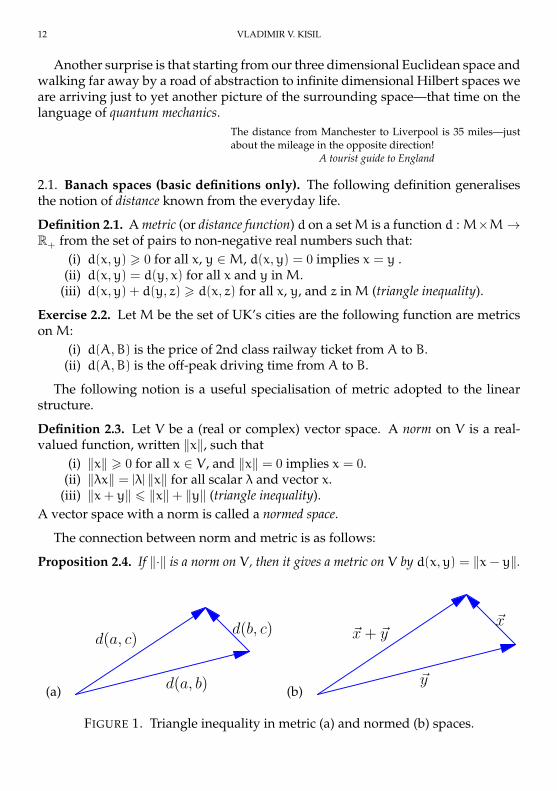
Proposition 2.4. If ‖·‖ is a norm on V , then it gives a metric on V by d(x,y) = ‖x− y‖.
(a)
d(a, c)
d(a, b)
d(b, c)
(b)
~x+ ~y
~y
~x
FIGURE 1. Triangle inequality in metric (a) and normed (b) spaces.
INTRODUCTION TO FUNCTIONAL ANALYSIS 13
Proof. This is a simple exercise to derive items 2.1(i)–2.1(iii) of Definition 2.1 fromcorresponding items of Definition 2.3. For example, see the Figure 1 to derive thetriangle inequality.
An important notions known from real analysis are limit and convergence. Par-ticularly we usually wish to have enough limiting points for all “reasonable” se-quences.
Definition 2.5. A sequence xk in a metric space (M,d) is a Cauchy sequence, if forevery ε > 0, there exists an integer n such that k, l > n implies that d(xk, xl) < ε.
Definition 2.6. (M,d) is a complete metric space if every Cauchy sequence inM con-verges to a limit inM.
For example, the set of integers Z and reals R with the natural distance functionsare complete spaces, but the set of rationals Q is not. The complete normed spacesdeserve a special name.
Definition 2.7. A Banach space is a complete normed space.
Exercise∗ 2.8. A convenient way to define a norm in a Banach space is as follows.The unit ball Uin a normed space B is the set of x such that ‖x‖ 6 1. Prove that:
(i) U is a convex set, i.e. x, y ∈ U and λ ∈ [0, 1] the point λx+ (1− λ)y is also inU.
(ii) ‖x‖ = infλ ∈ R+ | λ−1x ∈ U.(iii) U is closed if and only if the space is Banach.
Example 2.9. Here is some examples of normed spaces.(i) `n2 is either Rn or Cn with norm defined by
‖(x1, . . . , xn)‖2 =
√|x1|
2 + |x2|2 + · · ·+ |xn|
2.
(ii) `n1 is either Rn or Cn with norm defined by
‖(x1, . . . , xn)‖1 = |x1|+ |x2|+ · · ·+ |xn|.
(iii) `n∞ is either Rn or Cn with norm defined by
‖(x1, . . . , xn)‖∞ = max(|x1| , |x2| , · · · , |xn|).
(iv) LetX be a topological space, thenCb(X) is the space of continuous boundedfunctions f : X→ C with norm ‖f‖∞ = supX |f(x)|.
(v) Let X be any set, then `∞(X) is the space of all bounded (not necessarilycontinuous) functions f : X→ C with norm ‖f‖∞ = supX |f(x)|.
All these normed spaces are also complete and thus are Banach spaces. Some moreexamples of both complete and incomplete spaces shall appear later.
—We need an extra space to accommodate this product!A manager to a shop assistant

14 VLADIMIR V. KISIL
(i)
1
1
(ii)
1
1
(iii)
1
1
FIGURE 2. Different unit balls defining norms in R2 from Example 2.9.
2.2. Hilbert spaces. Although metric and norm capture important geometric in-formation about linear spaces they are not sensitive enough to represent such geo-metric characterisation as angles (particularly orthogonality). To this end we need afurther refinements.
From courses of linear algebra known that the scalar product 〈x,y〉 = x1y1 +
· · · + xnyn is important in a space Rn and defines a norm ‖x‖2 = 〈x, x〉. Here is asuitable generalisation:
Definition 2.10. A scalar product (or inner product) on a real or complex vector spaceV is a mapping V × V → C, written 〈x,y〉, that satisfies:
(i) 〈x, x〉 > 0 and 〈x, x〉 = 0 implies x = 0.(ii) 〈x,y〉 = 〈y, x〉 in complex spaces and 〈x,y〉 = 〈y, x〉 in real ones for all x,
y ∈ V .(iii) 〈λx,y〉 = λ 〈x,y〉, for all x, y ∈ V and scalar λ. (What is 〈x, λy〉?).

INTRODUCTION TO FUNCTIONAL ANALYSIS 15
(iv) 〈x+ y, z〉 = 〈x, z〉+ 〈y, z〉, for all x, y, and z ∈ V . (What is 〈x,y+ z〉?).
Last two properties of the scalar product is oftenly encoded in the phrase: “it islinear in the first variable if we fix the second and anti-linear in the second if we fixthe first”.
Definition 2.11. An inner product space V is a real or complex vector space with ascalar product on it.
Example 2.12. Here is some examples of inner product spaces which demonstratethat expression ‖x‖ =
√〈x, x〉 defines a norm.
(i) The inner product for Rn was defined in the beginning of this section.The inner product for Cn is given by 〈x,y〉 = ∑n
1 xjyj. The norm ‖x‖ =√∑n1 |xj|
2 makes it `n2 from Example 2.9(i).(ii) The extension for infinite vectors: let `2 be
(2.2) `2 = sequences xj∞1 |
∞∑1
|xj|2 <∞.
Let us equip this set with operations of term-wise addition and multiplic-ation by scalars, then `2 is closed under them. Indeed it follows from thetriangle inequality and properties of absolutely convergent series. Fromthe standard Cauchy–Bunyakovskii–Schwarz inequality follows that theseries
∑∞1 xjyj absolutely converges and its sum defined to be 〈x,y〉.
(iii) Let Cb[a,b] be a space of continuous functions on the interval [a,b] ∈ R.As we learn from Example 2.9(iv) a normed space it is a normed space withthe norm ‖f‖∞ = sup[a,b] |f(x)|. We could also define an inner product:
(2.3) 〈f,g〉 =b∫a
f(x)g(x)dx and ‖f‖2 =
b∫a
|f(x)|2 dx
12
.
Now we state, probably, the most important inequality in analysis.
Theorem 2.13 (Cauchy–Schwarz–Bunyakovskii inequality). For vectors x and y inan inner product space V let us define ‖x‖ =
√〈x, x〉 and ‖y‖ =
√〈y,y〉 then we have
(2.4) |〈x,y〉| 6 ‖x‖ ‖y‖ ,
with equality if and only if x and y are scalar multiple each other.
Proof. For any x, y ∈ V and any t ∈ R we have:
0 < 〈x+ ty, x+ ty〉 = 〈x, x〉+ 2t< 〈y, x〉+ t2 〈y,y〉),Thus the discriminant of this quadratic expression in t is non-positive: (< 〈y, x〉)2−‖x‖2 ‖y‖2 6 0, that is |< 〈x,y〉| 6 ‖x‖ ‖y‖. Replacing y by eiαy for an arbitraryα ∈ [−π,π] we get
∣∣<(eiα 〈x,y〉)∣∣ 6 ‖x‖ ‖y‖, this implies the desired inequality.

16 VLADIMIR V. KISIL
Corollary 2.14. Any inner product space is a normed space with norm ‖x‖ =√〈x, x〉
(hence also a metric space, Prop. 2.4).
Proof. Just to check items 2.3(i)–2.3(iii) from Definition 2.3.
Again complete inner product spaces deserve a special name
Definition 2.15. A complete inner product space is Hilbert space.
The relations between spaces introduced so far are as follows:Hilbert spaces ⇒ Banach spaces ⇒ Complete metric spaces
⇓ ⇓ ⇓inner product spaces ⇒ normed spaces ⇒ metric spaces.
How can we tell if a given norm comes from an inner product?
~x ~x
~y
~y
~x− ~y
~x+ ~y
FIGURE 3. To the parallelogram identity.
Theorem 2.16 (Parallelogram identity). In an inner product space H we have for all xand y ∈ H (see Figure 3):
(2.5) ‖x+ y‖2 + ‖x− y‖2 = 2 ‖x‖2 + 2 ‖y‖2 .
Proof. Just by linearity of inner product:
〈x+ y, x+ y〉+ 〈x− y, x− y〉 = 2 〈x, x〉+ 2 〈y,y〉 ,because the cross terms cancel out.
Exercise 2.17. Show that (2.5) is also a sufficient condition for a norm to arise froman inner product. Namely, for a norm on a complex Banach space satisfying to (2.5)the formula
〈x,y〉 =1
4
(‖x+ y‖2 − ‖x− y‖2 + i ‖x+ iy‖2 − i ‖x− iy‖2
)(2.6)
=1
4
3∑0
ik∥∥x+ iky∥∥2
defines an inner product. What is a suitable formula for a real Banach space?

INTRODUCTION TO FUNCTIONAL ANALYSIS 17
Divide and rule!Old but still much used recipe
2.3. Subspaces. To study Hilbert spaces we may use the traditional mathematicaltechnique of analysis and synthesis: we split the initial Hilbert spaces into smallerand probably simpler subsets, investigate them separately, and then reconstruct theentire picture from these parts.
As known from the linear algebra, a linear subspace is a subset of a linear spaceis its subset, which inherits the linear structure, i.e. possibility to add vectors andmultiply them by scalars. In this course we need also that subspaces inherit topo-logical structure (coming either from a norm or an inner product) as well.
Definition 2.18. By a subspace of a normed space (or inner product space) we meana linear subspace with the same norm (inner product respectively). We write X ⊂ Yor X ⊆ Y.
Example 2.19. (i) Cb(X) ⊂ `∞(X) where X is a metric space.(ii) Any linear subspace of Rn or Cn with any norm given in Example 2.9(i)–
2.9(iii).(iii) Let c00 be the space of finite sequences, i.e. all sequences (xn) such that exist
N with xn = 0 for n > N. This is a subspace of `2 since∑∞
1 |xj|2 is a finite
sum, so finite.
We also wish that the both inhered structures (linear and topological) should bein agreement, i.e. the subspace should be complete. Such inheritance is linked tothe property be closed.
A subspace need not be closed—for example the sequence
x = (1, 1/2, 1/3, 1/4, . . .) ∈ `2 because∑
1/k2 <∞and xn = (1, 1/2, . . . , 1/n, 0, 0, . . .) ∈ c00 converges to x thus x ∈ c00 ⊂ `2.
Proposition 2.20. (i) Any closed subspace of a Banach/Hilbert space is complete,hence also a Banach/Hilbert space.
(ii) Any complete subspace is closed.(iii) The closure of subspace is again a subspace.
Proof. (i) This is true in any metric space X: any Cauchy sequence from Y hasa limit x ∈ X belonging to Y, but if Y is closed then x ∈ Y.
(ii) Let Y is complete and x ∈ Y, then there is sequence xn → x in Y and it is aCauchy sequence. Then completeness of Y implies x ∈ Y.
(iii) If x, y ∈ Y then there are xn and yn in Y such that xn → x and yn → y.From the triangle inequality:
‖(xn + yn) − (x+ y)‖ 6 ‖xn − x‖+ ‖yn − y‖ → 0,
so xn+yn → x+y and x+y ∈ Y. Similarly x ∈ Y implies λx ∈ Y for any λ.

18 VLADIMIR V. KISIL
Hence c00 is an incomplete inner product space, with inner product 〈x,y〉 =∑∞1 xkyk (this is a finite sum!) as it is not closed in `2.
(a)1
1
12− 1
n12+ 1
n (b)
1
1
12
FIGURE 4. Jump function on (b) as a L2 limit of continuous func-tions from (a).
SimilarlyC[0, 1] with inner product norm ‖f‖ =(
1∫0
|f(t)|2 dt
)1/2
is incomplete—
take the large space X of functions continuous on [0, 1] except for a possible jump at12 (i.e. left and right limits exists but may be unequal and f(12 ) = limt→ 1
2+f(t). Then
the sequence of functions defined on Figure 4(a) has the limit shown on Figure 4(b)since:
‖f− fn‖ =
12+
1n∫
12−
1n
|f− fn|2 dt <
2
n→ 0.
Obviously f ∈ C[0, 1] \ C[0, 1].
Exercise 2.21. Show alternatively that the sequence of function fn from Figure 4(a)is a Cauchy sequence in C[0, 1] but has no continuous limit.

INTRODUCTION TO FUNCTIONAL ANALYSIS 19
Similarly the space C[a,b] is incomplete for any a < b if equipped by the innerproduct and the corresponding norm:
〈f,g〉 =
b∫a
f(t)g(t)dt(2.7)
‖f‖2 =
b∫a
|f(t)|2 dt
1/2
.(2.8)
Definition 2.22. Define a Hilbert space L2[a,b] to be the smallest complete innerproduct space containing space C[a,b] with the restriction of inner product givenby (2.7).
It is practical to realise L2[a,b] as a certain space of “functions” with the innerproduct defined via an integral. There are several ways to do that and we mentionjust two:
(i) Elements of L2[a,b] are equivalent classes of Cauchy sequences f(n) offunctions from C[a,b].
(ii) Let integration be extended from the Riemann definition to the wider Le-besgue integration (see Section 13). Let L be a set of square integrable inLebesgue sense functions on [a,b] with a finite norm (2.8). Then L2[a,b]is a quotient space of L with respect to the equivalence relation f ∼ g ⇔‖f− g‖2 = 0.
Example 2.23. Let the Cantor function on [0, 1] be defined as follows:
f(t) =
1, t ∈ Q;0, t ∈ R \Q.
This function is not integrable in the Riemann sense but does have the Le-besgue integral. The later however is equal to 0 and as an L2-function theCantor function equivalent to the function identically equal to 0.
(iii) The third possibility is to map L2(R) onto a space of “true” functions butwith an additional structure. For example, in quantum mechanics it is usefulto work with the Segal–Bargmann space of analytic functions on C with theinner product:
〈f1, f2〉 =∫Cf1(z)f2(z)e
−|z|2 dz.
Theorem 2.24. The sequence space `2 is complete, hence a Hilbert space.
Proof. Take a Cauchy sequence x(n) ∈ `2, where x(n) = (x(n)1 , x
(n)2 , x
(n)3 , . . .). Our
proof will have three steps: identify the limit x; show it is in `2; show x(n) → x.
20 VLADIMIR V. KISIL
(i) If x(n) is a Cauchy sequence in `2 then x(n)k is also a Cauchy sequence ofnumbers for any fixed k:∣∣∣x(n)k − x
(m)k
∣∣∣ 6 ( ∞∑k=1
∣∣∣x(n)k − x(m)k
∣∣∣2)1/2
=∥∥∥x(n) − x(m)
∥∥∥→ 0.
Let xk be the limit of x(n)k .(ii) For a given ε > 0 find n0 such that
∥∥x(n) − x(m)∥∥ < ε for all n,m > n0.
For any K andm:K∑k=1
∣∣∣x(n)k − x(m)k
∣∣∣2 6 ∥∥∥x(n) − x(m)∥∥∥2 < ε2.
Letm→∞ then∑Kk=1
∣∣∣x(n)k − xk
∣∣∣2 6 ε2.
Let K → ∞ then∑∞k=1
∣∣∣x(n)k − xk
∣∣∣2 6 ε2. Thus x(n) − x ∈ `2 and because
`2 is a linear space then x = x(n) − (x(n) − x) is also in `2.(iii) We saw above that for any ε > 0 there is n0 such that
∥∥x(n) − x∥∥ < ε forall n > n0. Thus x(n) → x.
Consequently `2 is complete.
All good things are covered by a thick layer of chocolate (well,if something is not yet–it certainly will)
2.4. Linear spans. As was explained into introduction 2, we describe “internal”properties of a vector through its relations to other vectors. For a detailed descrip-tion we need sufficiently many external reference points.
Let A be a subset (finite or infinite) of a normed space V . We may wish to up-grade it to a linear subspace in order to make it subject to our theory.
Definition 2.25. The linear span of A, write Lin(A), is the intersection of all linearsubspaces of V containing A, i.e. the smallest subspace containing A, equivalentlythe set of all finite linear combination of elements of A. The closed linear span of Awrite CLin(A) is the intersection of all closed linear subspaces of V containingA, i.e.the smallest closed subspace containing A.
Exercise∗ 2.26. (i) Show that if A is a subset of finite dimension space thenLin(A) = CLin(A).
(ii) Show that for an infinite A spaces Lin(A) and CLin(A)could be different.(Hint: use Example 2.19(iii).)
Proposition 2.27. Lin(A) = CLin(A).

INTRODUCTION TO FUNCTIONAL ANALYSIS 21
Proof. Clearly Lin(A) is a closed subspace containingA thus it should contain CLin(A).Also Lin(A) ⊂ CLin(A) thus Lin(A) ⊂ CLin(A) = CLin(A). Therefore Lin(A) =CLin(A).
Consequently CLin(A) is the set of all limiting points of finite linear combinationof elements of A.
Example 2.28. Let V = C[a,b] with the sup norm ‖·‖∞. Then:Lin1, x, x2, . . . = all polynomialsCLin1, x, x2, . . . = C[a,b] by the Weierstrass approximation theorem proved later.
The following simple result will be used later many times without comments.
Lemma 2.29 (about Inner Product Limit). Suppose H is an inner product space andsequences xn and yn have limits x and y correspondingly. Then 〈xn,yn〉 → 〈x,y〉 orequivalently:
limn→∞ 〈xn,yn〉 =
⟨limn→∞ xn, lim
n→∞yn⟩
.
Proof. Obviously by the Cauchy–Schwarz inequality:
|〈xn,yn〉− 〈x,y〉| = |〈xn − x,yn〉+ 〈x,yn − y〉|6 |〈xn − x,yn〉|+ |〈x,yn − y〉|6 ‖xn − x‖ ‖yn‖+ ‖x‖ ‖yn − y‖ → 0,
since ‖xn − x‖ → 0, ‖yn − y‖ → 0, and ‖yn‖ is bounded.
3. ORTHOGONALITY
Pythagoras is forever!The catchphrase from TV commercial of Hilbert Spaces course
As was mentioned in the introduction the Hilbert spaces is an analog of our 3DEuclidean space and theory of Hilbert spaces similar to plane or space geometry.One of the primary result of Euclidean geometry which still survives in high schoolcurriculum despite its continuous nasty de-geometrisation is Pythagoras’ theorembased on the notion of orthogonality1.
So far we was concerned only with distances between points. Now we wouldlike to study angles between vectors and notably right angles. Pythagoras’ theoremstates that if the angle C in a triangle is right then c2 = a2 + b2, see Figure 5 .
It is a very mathematical way of thinking to turn this property of right angles intotheir definition, which will work even in infinite dimensional Hilbert spaces.
Look for a triangle, or even for a right triangleA universal advice in solving problems from elementary
geometry.
1Some more “strange” types of orthogonality can be seen in the paper Elliptic, Parabolic and HyperbolicAnalytic Function Theory–1: Geometry of Invariants.

22 VLADIMIR V. KISIL
a
bc
FIGURE 5. The Pythagoras’ theorem c2 = a2 + b2
3.1. Orthogonal System in Hilbert Space. In inner product spaces it is even moreconvenient to give a definition of orthogonality not from Pythagoras’ theorem butfrom an equivalent property of inner product.
Definition 3.1. Two vectors x and y in an inner product space are orthogonal if〈x,y〉 = 0, written x ⊥ y.
An orthogonal sequence (or orthogonal system) en (finite or infinite) is one in whichen ⊥ em whenever n 6= m.
An orthonormal sequence (or orthonormal system) en is an orthogonal sequencewith ‖en‖ = 1 for all n.
Exercise 3.2. (i) Show that if x ⊥ x then x = 0 and consequently x ⊥ y for anyy ∈ H.
(ii) Show that if all vectors of an orthogonal system are non-zero then they arelinearly independent.
Example 3.3. These are orthonormal sequences:(i) Basis vectors (1, 0, 0), (0, 1, 0), (0, 0, 1) in R3 or C3.
(ii) Vectors en = (0, . . . , 0, 1, 0, . . .) (with the only 1 on the nth place) in `2.(Could you see a similarity with the previous example?)
(iii) Functions en(t) = 1/(√
2π)eint , n ∈ Z in C[0, 2π]:
(3.1) 〈en, em〉 =2π∫0
1
2πeinte−imtdt =
1, n = m;0, n 6= m.
Exercise 3.4. LetA be a subset of an inner product space V and x ⊥ y for any y ∈ A.Prove that x ⊥ z for all z ∈ CLin(A).
Theorem 3.5 (Pythagoras’). If x ⊥ y then ‖x+ y‖2 = ‖x‖2 + ‖y‖2. Also if e1, . . . , enis orthonormal then∥∥∥∥∥
n∑1
akek
∥∥∥∥∥2
=
⟨n∑1
akek,
n∑1
akek
⟩=
n∑1
|ak|2 .

INTRODUCTION TO FUNCTIONAL ANALYSIS 23
Proof. A one-line calculation.
The following theorem provides an important property of Hilbert spaces whichwill be used many times. Recall, that a subset K of a linear space V is convex if for allx, y ∈ K and λ ∈ [0, 1] the point λx+ (1− λ)y is also in K. Particularly any subspaceis convex and any unit ball as well (see Exercise 2.8(i)).
Theorem 3.6 (about the Nearest Point). Let K be a non-empty convex closed subset of aHilbert space H. For any point x ∈ H there is the unique point y ∈ K nearest to x.
Proof. Let d = infy∈K d(x,y), where d(x,y)—the distance coming from the norm‖x‖ =
√〈x, x〉 and let yn a sequence points in K such that limn→∞ d(x,yn) = d.
Then yn is a Cauchy sequence. Indeed from the parallelogram identity for theparallelogram generated by vectors x− yn and x− ym we have:
‖yn − ym‖2 = 2 ‖x− yn‖2 + 2 ‖x− ym‖2 − ‖2x− yn − ym‖2 .
Note that ‖2x− yn − ym‖2 = 4∥∥x− yn+ym
2
∥∥2 > 4d2 since yn+ym
2 ∈ K by its con-vexity. For sufficiently large m and n we get ‖x− ym‖2 6 d + ε and ‖x− yn‖2 6d+ ε, thus ‖yn − ym‖ 6 4(d2 + ε) − 4d2 = 4ε, i.e. yn is a Cauchy sequence.
Let y be the limit of yn, which exists by the completeness of H, then y ∈ Ksince K is closed. Then d(x,y) = limn→∞ d(x,yn) = d. This show the existenceof the nearest point. Let y ′ be another point in K such that d(x,y ′) = d, then theparallelogram identity implies:
‖y− y ′‖2 = 2 ‖x− y‖2 + 2 ‖x− y ′‖2 − ‖2x− y− y ′‖2 6 4d2 − 4d2 = 0.
This shows the uniqueness of the nearest point.
Exercise∗ 3.7. The essential role of the parallelogram identity in the above proofindicates that the theorem does not hold in a general Banach space.
(i) Show that in R2 with either norm ‖·‖1 or ‖·‖∞ form Example 2.9 the nearestpoint could be non-unique;
(ii) Could you construct an example (in Banach space) when the nearest pointdoes not exists?
Liberte, Egalite, Fraternite!A longstanding ideal approximated in the real life by
something completely different
3.2. Bessel’s inequality. For the case then a convex subset is a subspace we couldcharacterise the nearest point in the term of orthogonality.
Theorem 3.8 (on Perpendicular). Let M be a subspace of a Hilbert space H and a pointx ∈ H be fixed. Then z ∈ M is the nearest point to x if and only if x − z is orthogonal toany vector inM.

24 VLADIMIR V. KISIL
Proof. Let z is the nearest point to x existing by the previous Theorem. We claimthat x − z orthogonal to any vector in M, otherwise there exists y ∈ M such that〈x− z,y〉 6= 0. Then
‖x− z− εy‖2 = ‖x− z‖2 − 2ε< 〈x− z,y〉+ ε2 ‖y‖2
< ‖x− z‖2 ,
if ε is chosen to be small enough and such that ε< 〈x− z,y〉 is positive, see Fig-ure 6(i). Therefore we get a contradiction with the statement that z is closest pointto x.
On the other hand if x − z is orthogonal to all vectors in H1 then particularly(x − z) ⊥ (z − y) for all y ∈ H1, see Figure 6(ii). Since x − y = (x − z) + (z − y) wegot by the Pythagoras’ theorem:
‖x− y‖2 = ‖x− z‖2 + ‖z− y‖2 .
So ‖x− y‖2 > ‖x− z‖2 and the are equal if and only if z = y.
(i)
M
x
zǫy (ii)
e1
e2z
x
y
FIGURE 6. (i) A smaller distance for a non-perpendicular direction;and(ii) Best approximation from a subspace
Exercise 3.9. The above proof does not work if 〈x− z,y〉 is an imaginary number,what to do in this case?
Consider now a basic case of approximation: let x ∈ H be fixed and e1, . . . , en beorthonormal and denote H1 = Line1, . . . , en. We could try to approximate x by avector y = λ1e1 + · · ·+ λnen ∈ H1.
Corollary 3.10. The minimal value of ‖x− y‖ for y ∈ H1 is achieved when y =∑n
1 〈x, ei〉 ei.Proof. Let z =
∑n1 〈x, ei〉 ei, then 〈x− z, ei〉 = 〈x, ei〉 − 〈z, ei〉 = 0. By the previous
Theorem z is the nearest point to x.

INTRODUCTION TO FUNCTIONAL ANALYSIS 25
Example 3.11. (i) In R3 find the best approximation to (1, 0, 0) from the planeV : x1+x2+x3 = 0. We take an orthonormal basis e1 = (2−1/2,−2−1/2, 0),e2 = (6−1/2, 6−1/2,−2 · 6−1/2) of V (Check this!). Then:
z = 〈x, e1〉 e1 + 〈x, e2〉 e2 =
(1
2,−
1
2, 0
)+
(1
6,
1
6,−
1
3
)=
(2
3,−
1
3,−
1
3
).
(ii) In C[0, 2π] what is the best approximation to f(t) = t by functions a +beit + ce−it? Let
e0 =1√2π
, e1 =1√2πeit, e−1 =
1√2πe−it.
We find:
〈f, e0〉 =
2π∫0
t√2πdt =
[t2
2
1√2π
]2π0
=√
2π3/2;
〈f, e1〉 =
2π∫0
te−it√2πdt = i
√2π (Check this!)
〈f, e−1〉 =
2π∫0
teit√2πdt = −i
√2π (Why we may not check this one?)
Then the best approximation is (see Figure 7):
f0(t) = 〈f, e0〉 e0 + 〈f, e1〉 e1 + 〈f, e−1〉 e−1
=
√2π3/2√
2π+ ieit − ie−it = π− 2 sin t.
0
6.3
y
0 6.3x
FIGURE 7. Best approximation by three trigonometric polynomials

26 VLADIMIR V. KISIL
Corollary 3.12 (Bessel’s inequality). If (ei) is orthonormal then
‖x‖2 >n∑i=1
|〈x, ei〉|2 .
Proof. Let z =∑n
1 〈x, ei〉ei then x−z ⊥ ei for all i therefore by Exercise 3.4 x−z ⊥ z.Hence:
‖x‖2 = ‖z‖2 + ‖x− z‖2
> ‖z‖2 =
n∑i=1
|〈x, ei〉|2 .
—Did you say “rice and fish for them”?
A student question
3.3. The Riesz–Fischer theorem. When (ei) is orthonormal we call 〈x, en〉 the nthFourier coefficient of x (with respect to (ei), naturally).
Theorem 3.13 (Riesz–Fisher). Let (en)∞1 be an orthonormal sequence in a Hilbert spaceH. Then
∑∞1 λnen converges inH if and only if
∑∞1 |λn|
2 <∞. In this case ‖∑∞1 λnen‖2 =∑∞1 |λn|
2.
Proof. Necessity: Let xk =∑k
1 λnen and x = limk→∞ xk. So 〈x, en〉 = limk→∞ 〈xk, en〉 =λn for all n. By the Bessel’s inequality for all k
‖x‖2 >k∑1
|〈x, en〉|2 =
k∑1
|λn|2 ,
hence∑k
1 |λn|2 converges and the sum is at most ‖x‖2.
Sufficiency: Consider ‖xk − xm‖ =∥∥∥∑k
m λnen
∥∥∥ =(∑k
m |λn|2)1/2
for k > m.
Since∑km |λn|
2 converges xk is a Cauchy sequence in H and thus has a limit x. Bythe Pythagoras’ theorem ‖xk‖2 =
∑k1 |λn|
2 thus for k→∞ ‖x‖2 =∑∞
1 |λn|2 by the
Lemma about inner product limit.
Observation: the closed linear span of an orthonormal sequence in any Hilbertspace looks like `2, i.e. `2 is a universal model for a Hilbert space.
By Bessel’s inequality and the Riesz–Fisher theorem we know that the series∑∞1 〈x, ei〉 ei converges for any x ∈ H. What is its limit?Let y = x−
∑∞1 〈x, ei〉 ei, then
(3.2) 〈y, ek〉 = 〈x, ek〉−∞∑1
〈x, ei〉 〈ei, ek〉 = 〈x, ek〉− 〈x, ek〉 = 0 for all k.

INTRODUCTION TO FUNCTIONAL ANALYSIS 27
Definition 3.14. An orthonormal sequence (ei) in a Hilbert space H is complete ifthe identities 〈y, ek〉 = 0 for all k imply y = 0.
A complete orthonormal sequence is also called orthonormal basis in H.
Theorem 3.15 (on Orthonormal Basis). Let ei be an orthonormal basis in a Hilber spaceH. Then for any x ∈ H we have
x =
∞∑n=1
〈x, en〉 en and ‖x‖2 =
∞∑n=1
|〈x, en〉|2 .
Proof. By the Riesz–Fisher theorem, equation (3.2) and definition of orthonormalbasis.
There are constructive existence theorems in mathematics.An example of pure existence statement
3.4. Construction of Orthonormal Sequences. Natural questions are: Do orthonor-mal sequences always exist? Could we construct them?
Theorem 3.16 (Gram–Schmidt). Let (xi) be a sequence of linearly independent vectorsin an inner product space V . Then there exists orthonormal sequence (ei) such that
Linx1, x2, . . . , xn = Line1, e2, . . . , en, for all n.
Proof. We give an explicit algorithm working by induction. The base of induction:the first vector is e1 = x1/ ‖x1‖. The step of induction: let e1, e2, . . . , en are alreadyconstructed as required. Let yn+1 = xn+1−
∑ni=1 〈xn+1, ei〉 ei. Then by (3.2) yn+1 ⊥
ei for i = 1, . . . ,n. We may put en+1 = yn+1/ ‖yn+1‖ because yn+1 6= 0 due tolinear independence of xk’s. Also
Line1, e2, . . . , en+1 = Line1, e2, . . . ,yn+1
= Line1, e2, . . . , xn+1
= Linx1, x2, . . . , xn+1.
So (ei) are orthonormal sequence.
Example 3.17. Consider C[0, 1] with the usual inner product (2.7) and apply ortho-gonalisation to the sequence 1, x, x2, . . . . Because ‖1‖ = 1 then e1(x) = 1. Thecontinuation could be presented by the table:
e1(x) = 1
y2(x) = x− 〈x, 1〉 1 = x−1
2, ‖y2‖2 =
1∫0
(x−1
2)2 dx =
1
12, e2(x) =
√12(x−
1
2)
y3(x) = x2 −
⟨x2, 1
⟩1 −
⟨x2, x−
1
2
⟩(x−
1
2) · 12, . . . , e3 =
y3
‖y3‖. . . . . . . . .

28 VLADIMIR V. KISIL
Example 3.18. Many famous sequences of orthogonal polynomials, e.g. Cheby-shev, Legendre, Laguerre, Hermite, can be obtained by orthogonalisation of 1, x,x2, . . . with various inner products.
(i) Legendre polynomials in C[−1, 1] with inner product
(3.3) 〈f,g〉 =1∫
−1
f(t)g(t)dt.
(ii) Chebyshev polynomials in C[−1, 1] with inner product
(3.4) 〈f,g〉 =1∫
−1
f(t)g(t)dt√
1 − t2
(iii) Laguerre polynomials in the space of polynomials P[0,∞) with inner product
〈f,g〉 =∞∫0
f(t)g(t)e−t dt.
−1 0 1x
−1
0
1
y
−1 0 1x
−1
0
1
y
FIGURE 8. Five first Legendre Pi and Chebyshev Ti polynomials
See Figure 8 for the five first Legendre and Chebyshev polynomials. Observe thedifference caused by the different inner products (3.3) and (3.4). On the other handnote the similarity in oscillating behaviour with different “frequencies”.
Another natural question is: When is an orthonormal sequence complete?
Proposition 3.19. Let (en) be an orthonormal sequence in a Hilbert space H. The follow-ing are equivalent:

INTRODUCTION TO FUNCTIONAL ANALYSIS 29
(i) (en) is an orthonormal basis.(ii) CLin((en)) = H.
(iii) ‖x‖2 =∑∞
1 |〈x, en〉|2 for all x ∈ H.
Proof. Clearly 3.19(i) implies 3.19(ii) because x =∑∞
1 〈x, en〉 en in CLin((en)) and‖x‖2 =
∑∞1 〈x, en〉 en by Theorem 3.15.
If (en) is not complete then there exists x ∈ H such that x 6= 0 and 〈x, ek〉 for allk, so 3.19(iii) fails, consequently 3.19(iii) implies 3.19(i).
Finally if 〈x, ek〉 = 0 for all k then 〈x,y〉 = 0 for all y ∈ Lin((en)) and moreoverfor all y ∈ CLin((en)), by the Lemma on continuity of the inner product. But thenx 6∈ CLin((en)) and 3.19(ii) also fails because 〈x, x〉 = 0 is not possible. Thus 3.19(ii)implies 3.19(i).
Corollary 3.20. A separable Hilbert space (i.e. one with a countable dense set) can beidentified with either `n2 or `2, in other words it has an orthonormal basis (en) (finite orinfinite) such that
x =
∞∑n=1
〈x, en〉 en and ‖x‖2 =
∞∑n=1
|〈x, en〉|2 .
Proof. Take a countable dense set (xk), then H = CLin((xk)), delete all vectorswhich are a linear combinations of preceding vectors, make orthonormalisation byGram–Schmidt the remaining set and apply the previous proposition.
Most pleasant compliments are usually orthogonal to our realqualities.
An advise based on observations
3.5. Orthogonal complements.
Definition 3.21. Let M be a subspace of an inner product space V . The orthogonalcomplement, writtenM⊥, ofM is
M⊥ = x ∈ V : 〈x,m〉 = 0 ∀m ∈M.
Theorem 3.22. IfM is a closed subspace of a Hilbert spaceH thenM⊥ is a closed subspacetoo (hence a Hilbert space too).
Proof. ClearlyM⊥ is a subspace of H because x, y ∈M⊥ implies ax+ by ∈M⊥:
〈ax+ by,m〉 = a 〈x,m〉+ b 〈y,m〉 = 0.
Also if all xn ∈ M⊥ and xn → x then x ∈ M⊥ due to inner product limit Lemma.
Theorem 3.23. Let M be a closed subspace of a Hilber space H. Then for any x ∈ Hthere exists the unique decomposition x = m + n with m ∈ M, n ∈ M⊥ and ‖x‖2 =
‖m‖2 + ‖n‖2. Thus H =M⊕M⊥ and (M⊥)⊥ =M.

30 VLADIMIR V. KISIL
Proof. For a given x there exists the unique closest pointm inM by the Theorem onnearest point and by the Theorem on perpendicular (x−m) ⊥ y for all y ∈M.
So x = m + (x −m) = m + n with m ∈ M and n ∈ M⊥. The identity ‖x‖2 =
‖m‖2 + ‖n‖2 is just Pythagoras’ theorem and M ∩M⊥ = 0 because null vector isthe only vector orthogonal to itself.
Finally (M⊥)⊥ =M. We haveH =M⊕M⊥ = (M⊥)⊥⊕M⊥, for any x ∈ (M⊥)⊥
there is a decomposition x = m + n with m ∈ M and n ∈ M⊥, but then n isorthogonal to itself and therefore is zero.
Corollary 3.24 (about Orthoprojection). There is a linear map PM from H ontoM (theorthogonal projection or orthoprojection) such that
(3.5) P2M = PM, kerPM =M⊥, PM⊥ = I− PM.
Proof. Let us define PM(x) = m where x = m + n is the decomposition from theprevious theorem. The linearity of this operator follows from the fact that both MandM⊥ are linear subspaces. Also PM(m) = m for allm ∈M and the image of PMis M. Thus P2M = PM. Also if PM(x) = 0 then x ⊥ M, i.e. kerPM = M⊥. SimilarlyPM⊥(x) = nwhere x = m+ n and PM + PM⊥ = I.
Example 3.25. Let (en) be an orthonormal basis in a Hilber space and let S ⊂ N befixed. LetM = CLinen : n ∈ S andM⊥ = CLinen : n ∈ N \ S. Then∞∑
k=1
akek =∑k∈S
akek +∑k6∈S
akek.
Remark 3.26. In fact there is a one-to-one correspondence between closed linearsubspaces of a Hilber spaceH and orthogonal projections defined by identities (3.5).
4. FOURIER ANALYSIS
All bases are equal, but some are more equal then others.
As we saw already any separable Hilbert space posses an orthonormal basis(infinitely many of them indeed). Are they equally good? This depends from ourpurposes. For solution of differential equation which arose in mathematical physics(wave, heat, Laplace equations, etc.) there is a proffered choice. The fundamentalformula: d
dxeax = aeax reduces the derivative to a multiplication by a. We could
benefit from this observation if the orthonormal basis will be constructed out ofexponents. This helps to solve differential equations as was demonstrated in Sub-section 1.2.
7.40pm Fourier series: Episode IIToday’s TV listing

INTRODUCTION TO FUNCTIONAL ANALYSIS 31
4.1. Fourier series. Now we wish to address questions stated in Remark 1.9. Let usconsider the space L2[−π,π]. As we saw in Example 3.3(iii) there is an orthonormalsequence en(t) = (2π)−1/2eint in L2[−π,π]. We will show that it is an orthonormalbasis, i.e.
f(t) ∈ L2[−π,π] ⇔ f(t) =
∞∑k=−∞ 〈f, ek〉 ek(t),
with convergence in L2 norm. To do this we show that CLinek : k ∈ Z = L2[−π,π].Let CP[−π,π] denote the continuous functions f on [−π,π] such that f(π) =
f(−π). We also define f outside of the interval [−π,π] by periodicity.
Lemma 4.1. The space CP[−π,π] is dense in L2[−π,π].
Proof. Let f ∈ L2[−π,π]. Given ε > 0 there exists g ∈ C[−π,π] such that ‖f− g‖ <ε/2. Form continuity of g on a compact set follows that there isM such that |g(t)| <M for all t ∈ [−π,π]. We can now replace g by periodic g, which coincides with
δ−π π
FIGURE 9. A modification of continuous function to periodic
g on [−π,π − δ] for an arbitrary δ > 0 and has the same bounds: |g(t)| < M, seeFigure 9. Then
‖g− g‖22 =
π∫π−δ
|g(t) − g(t)|2 dt 6 (2M)2δ.
So if δ < ε2/(4M)2 then ‖g− g‖ < ε/2 and ‖f− g‖ < ε.
Now if we could show that CLinek : k ∈ Z includes CP[−π,π] then it alsoincludes L2[−π,π].
Notation 4.2. Let f ∈ CP[−π,π],write
(4.1) fn =
n∑k=−n
〈f, ek〉 ek, for n = 0, 1, 2, . . .
the partial sum of the Fourier series for f.

32 VLADIMIR V. KISIL
We want to show that ‖f− fn‖2 → 0. To this end we define nth Fejer sum by theformula
(4.2) Fn =f0 + f1 + · · ·+ fn
n+ 1,
and show that‖Fn − f‖∞ → 0.
Then we conclude
‖Fn − f‖2 =
π∫−π
|Fn(t) − f|2
1/2
6 (2π)1/2 ‖Fn − f‖∞ → 0.
Since Fn ∈ Lin((en)) then f ∈ CLin((en)) and hence f =∑∞
−∞ 〈f, ek〉 ek.
Remark 4.3. It is not always true that ‖fn − f‖∞ → 0 even for f ∈ CP[−π,π].
Exercise 4.4. Find an example illustrating the above Remark.
It took 19 years of his life to prove this theorem
4.2. Fejer’s theorem.
Proposition 4.5 (Fejer, age 19). Let f ∈ CP[−π,π]. Then
Fn(x) =1
2π
π∫−π
f(t)Kn(x− t)dt, where(4.3)
Kn(t) =1
n+ 1
n∑k=0
k∑m=−k
eimt,(4.4)
is the Fejer kernel.
Proof. From notation (4.1):
fk(x) =
k∑m=−k
〈f, em〉 em(x)
=
k∑m=−k
π∫−π
f(t)e−imt√
2πdteimx√
2π
=1
2π
π∫−π
f(t)
k∑m=−k
eim(x−t) dt.

INTRODUCTION TO FUNCTIONAL ANALYSIS 33
Then from (4.2):
Fn(x) =1
n+ 1
n∑k=0
fk(x)
=1
n+ 1
1
2π
n∑k=0
π∫−π
f(t)
k∑m=−k
eim(x−t) dt
=1
2π
π∫−π
f(t)1
n+ 1
n∑k=0
k∑m=−k
eim(x−t) dt,
which finishes the proof.
Lemma 4.6. The Fejer kernel is 2π-periodic, Kn(0) = n+ 1 and:
(4.5) Kn(t) =1
n+ 1
sin2 (n+1)t2
sin2 t2
, for t 6∈ 2πZ.
Proof. Let z = eit, then:
Kn(t) =1
n+ 1
n∑k=0
(z−k + · · ·+ 1 + z+ · · ·+ zk)
=1
n+ 1
n∑j=−n
(n+ 1 − |j|)zj,
by switch from counting in rows to counting in columns in Table 1. Let w = eit/2,
1z−1 1 z
z−2 z−1 1 z z2
......
......
......
. . .
TABLE 1. Counting powers in rows and columns

34 VLADIMIR V. KISIL
i.e. z = w2, then
Kn(t) =1
n+ 1(w−2n + 2w−2n+2 + · · ·+ (n+ 1) + nw2 + · · ·+w2n)
=1
n+ 1(w−n +w−n+2 + · · ·+wn−2 +wn)2(4.6)
=1
n+ 1
(w−n−1 −wn+1
w−1 −w
)2
Could you sum a geometric progression?
=1
n+ 1
(2i sin (n+1)t
2
2i sin t2
)2
,
if w 6= ±1. For the value of Kn(0) we substitute w = 1 into (4.6).
The first eleven Fejer kernels are shown on Figure 10, we could observe that:
Lemma 4.7. Fejer’s kernel has the following properties:
−3 −2 −1 0 1 2 3x
−2
−1
0
1
2
3
4
5
6
7
8
9
y
−3 −2 −1 0 1 2 3x
−2
−1
0
1
2
3
4
5
6
7
8
9
y
FIGURE 10. A family of Fejer kernels with the parameter m run-ning from 0 to 9 is on the left picture. For a comparison unregular-ised Fourier kernels are on the right picture.

INTRODUCTION TO FUNCTIONAL ANALYSIS 35
(i) Kn(t) > 0 for all t ∈ R and n ∈ N.
(ii)π∫−π
Kn(t)dt = 2π.
(iii) For any δ ∈ (0,π)
−δ∫−π
+
π∫δ
Kn(t)dt→ 0 as n→∞.
Proof. The first property immediately follows from the explicit formula (4.5). Incontrast the second property is easier to deduce from expression with double sum (4.4):
π∫−π
Kn(t)dt =
π∫−π
1
n+ 1
n∑k=0
k∑m=−k
eimt dt
=1
n+ 1
n∑k=0
k∑m=−k
π∫−π
eimt dt
=1
n+ 1
n∑k=0
2π
= 2π,
since the formula (3.1).Finally if |t| > δ then sin2(t/2) > sin2(δ/2) > 0 by monotonicity of sinus on
[0,π/2], so:
0 6 Kn(t) 61
(n+ 1) sin2(δ/2)
implying:
0 6∫
δ6|t|6π
Kn(t)dt 61(π− δ)
(n+ 1) sin2(δ/2)→ 0 as n→ 0.
Therefore the third property follows from the squeeze rule.
Theorem 4.8 (Fejer Theorem). Let f ∈ CP[−π,π]. Then its Fejer sums Fn (4.2) con-verges in supremum norm to f on [−π,π] and hence in L2 norm as well.
Proof. Idea of the proof: if in the formula (4.3)
Fn(x) =1
2π
π∫−π
f(t)Kn(x− t)dt,
t is long way from x, Kn is small (see Lemma 4.7 and Figure 10), for t near x, Kn isbig with total “weight” 2π, so the weighted average of f(t) is near f(x).
36 VLADIMIR V. KISIL
Here are details. Using property 4.7(ii) and periodicity of f and Kn we couldexpress trivially
f(x) = f(x)1
2π
x+π∫x−π
Kn(x− t)dt =1
2π
x+π∫x−π
f(x)Kn(x− t)dt.
Similarly we rewrite (4.3) as
Fn(x) =1
2π
x+π∫x−π
f(t)Kn(x− t)dt,
then
|f(x) − Fn(x)| =1
2π
∣∣∣∣∣∣x+π∫x−π
(f(x) − f(t))Kn(x− t)dt
∣∣∣∣∣∣6
1
2π
x+π∫x−π
|f(x) − f(t)|Kn(x− t)dt.
Given ε > 0 split into three intervals: I1 = [x − π, x − δ], I2 = [x − δ, x + δ],I3 = [x + δ, x + π], where δ is chosen such that |f(t) − f(x)| < ε/2 for t ∈ I2, whichis possible by continuity of f. So
1
2π
∫I2
|f(x) − f(t)|Kn(x− t)dt 6ε
2
1
2π
∫I2
Kn(x− t)dt <ε
2.
And1
2π
∫I1∪I3
|f(x) − f(t)|Kn(x− t)dt 6 2 ‖f‖∞ 1
2π
∫I1∪I3
Kn(x− t)dt
=‖f‖∞π
∫δ<|u|<π
Kn(u)du
<ε
2,
if n is sufficiently large due to property 4.7(iii) of Kn. Hence |f(x) − Fn(x)| < ε for alarge n independent of x.
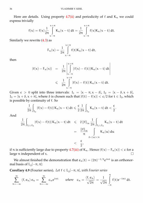
We almost finished the demonstration that en(t) = (2π)−1/2eint is an orthonor-mal basis of L2[−π,π]:
Corollary 4.9 (Fourier series). Let f ∈ L2[−π,π], with Fourier series∞∑
n=−∞ 〈f, en〉 en =
∞∑n=−∞ cne
int where cn =〈f, en〉√
2π=
1√2π
π∫−π
f(t)e−int dt.
INTRODUCTION TO FUNCTIONAL ANALYSIS 37
Then the series∑∞
−∞ 〈f, en〉 en =∑∞
−∞ cneint converges in L2[−π,π] to f, i.e
limk→∞
∥∥∥∥∥f−k∑
n=−k
cneint
∥∥∥∥∥2
= 0.
Proof. This follows from the previous Theorem, Lemma 4.1 about density of CP inL2, and Theorem 3.15 on orthonormal basis.
4.3. Parseval’s formula. The following result first appeared in the framework ofL2[−π,π] and only later was understood to be a general property of inner productspaces.
Theorem 4.10 (Parseval’s formula). If f, g ∈ L2[−π,π] have Fourier series f =∞∑
n=−∞ cneint
and g =
∞∑n=−∞dne
int, then
(4.7) 〈f,g〉 =π∫
−π
f(t)g(t)dt = 2π
∞∑−∞ cndn.
More generally if f and g are two vectors of a Hilbert spaceH with an orthonormal basis(en)
∞−∞ then
〈f,g〉 =∞∑
k=−∞ cndn, where cn = 〈f, en〉 , dn = 〈g, en〉 ,
are the Fourier coefficients of f and g.
Proof. In fact we could just prove the second, more general, statement—the firstone is its particular realisation. Let fn =
∑nk=−n ckek and gn =
∑nk=−n dkek will
be partial sums of the corresponding Fourier series. Then from orthonormality of(en) and linearity of the inner product:
〈fn,gn〉 =⟨
n∑k=−n
ckek,
n∑k=−n
dkek
⟩=
n∑k=−n
ckdk.
This formula together with the facts that fk → f and gk → g (following fromCorollary 4.9) and Lemma about continuity of the inner product implies the asser-tion.
Corollary 4.11. A integrable function f belongs to L2[−π,π] if and only if its Fourierseries is convergent and then ‖f‖2 = 2π
∑∞−∞ |ck|
2.
Proof. The necessity, i.e. implication f ∈ L2 ⇒ 〈f, f〉 = ‖f‖2 = 2π∑
|ck|2, follows
from the previous Theorem. The sufficiency follows by Riesz–Fisher Theorem.

38 VLADIMIR V. KISIL
Remark 4.12. The actual role of the Parseval’s formula is shadowed by the orthonor-mality and is rarely recognised until we meet the wavelets or coherent states. Indeedthe equality (4.7) should be read as follows:
Theorem 4.13 (Modified Parseval). The map W : H→ `2 given by the formula [Wf](n) =〈f, en〉 is an isometry for any orthonormal basis (en).
We could find many other systems of vectors (ex), x ∈ X (very different fromorthonormal bases) such that the map W : H→ L2(X) given by the simple universalformula
(4.8) [Wf](x) = 〈f, ex〉will be an isometry of Hilbert spaces. The map (4.8) is oftenly called wavelet trans-form and most famous is the Cauchy integral formula in complex analysis. The major-ity of wavelets transforms are linked with group representations, see our postgradu-ate course Wavelets in Applied and Pure Maths.
Heat and noise but not a fire?Answer: “ApplicationofFourierSeries”
4.4. Some Application of Fourier Series. We are going to provide now few ex-amples which demonstrate the importance of the Fourier series in many questions.The first two (Example 4.14 and Theorem 4.15) belong to pure mathematics and lasttwo are of more applicable nature.
Example 4.14. Let f(t) = t on [−π,π]. Then
〈f, en〉 =π∫
−π
te−int dt =
(−1)n 2πi
n, n 6= 0
0, n = 0(check!),
so f(t) ∼∑∞
−∞(−1)n(i/n)eint. By a direct integration:
‖f‖22 =
π∫−π
t2 dt =2π3
3.
On the other hand by the previous Corollary:
‖f‖22 = 2π∑n6=0
∣∣∣∣ (−1)ni
n
∣∣∣∣2 = 4π
∞∑n=1
1
n2.
Thus we get a beautiful formula ∞∑1
1
n2=π2
6.
Here is another important result.

INTRODUCTION TO FUNCTIONAL ANALYSIS 39
Theorem 4.15 (Weierstrass Approximation Theorem). For any function f ∈ C[a,b]and any ε > 0 there exists a polynomial p such that ‖f− p‖∞ < ε.
Proof. Change variable: t = 2π(x−a+b2 )/(b−a) this maps x ∈ [a,b] onto t ∈ [−π,π].Let P denote the subspace of polynomials in C[−π,π]. Then eint ∈ P for any n ∈ Zsince Taylor series converges uniformly in [−π,π]. Consequently P contains theclosed linear span in (supremum norm) of eint, any n ∈ Z, which is CP[−π,π] bythe Fejer theorem. Thus P ⊇ CP[−π,π] and we extend that to non-periodic functionas follows (why we could not make use of Lemma 4.1 here, by the way?).
For any f ∈ C[−π,π] let λ = (f(π)−f(−π))/(2π) then f1(t) = f(t)−λt ∈ CP[−π,π]and could be approximated by a polynomial p1(t) from the above discussion. Thenf(t) is approximated by the polynomial p(t) = p1(t) + λt.
It is easy to see, that the role of exponents eint in the above prove is rather mod-est: they can be replaced by any functions which has a Taylor expansion. The realglory of the Fourier analysis is demonstrated in the two following examples.
Example 4.16. The modern history of the Fourier analysis starts from the works ofFourier on the heat equation. As was mentioned in the introduction to this part, theexceptional role of Fourier coefficients for differential equations is explained by thesimple formula ∂xeinx = ineinx. We shortly review a solution of the heat equationto illustrate this.
Let we have a rod of the length 2π. The temperature at its point x ∈ [−π,π]and a moment t ∈ [0,∞) is described by a function u(t, x) on [0,∞)× [−π,π]. Themathematical equation describing a dynamics of the temperature distribution is:
(4.9)∂u(t, x)
∂t=∂2u(t, x)
∂x2or, equivalently,
(∂t − ∂
2x
)u(t, x) = 0.
For any fixed moment t0 the function u(t0, x) depends only from x ∈ [−π,π] andaccording to Corollary 4.9 could be represented by its Fourier series:
u(t0, x) =
∞∑n=−∞ 〈u, en〉 en =
∞∑n=−∞ cn(t0)e
inx,
where
cn(t0) =〈u, en〉√
2π=
1√2π
π∫−π
u(t0, x)e−inx dx,

40 VLADIMIR V. KISIL
with Fourier coefficients cn(t0) depending from t0. We substitute that decomposi-tion into the heat equation (4.9) to receive:(
∂t − ∂2x
)u(t, x) =
(∂t − ∂
2x
) ∞∑n=−∞ cn(t)e
inx
=
∞∑n=−∞
(∂t − ∂
2x
)cn(t)e
inx
=
∞∑n=−∞(c
′n(t) + n
2cn(t))einx = 0.(4.10)
Since function einx form a basis the last equation (4.10) holds if and only if
(4.11) c ′n(t) + n2cn(t) = 0 for all n and t.
FIGURE 11. The dynamics of a heat equation:x—coordinate on the rod,t—time,T—temperature.
Equations from the system (4.11) have general solutions of the form:
(4.12) cn(t) = cn(0)e−n2t for all t ∈ [0,∞),
producing a general solution of the heat equation (4.9) in the form:
(4.13) u(t, x) =
∞∑n=−∞ cn(0)e
−n2teinx =
∞∑n=−∞ cn(0)e
−n2t+inx,
where constant cn(0) could be defined from boundary condition. For example, ifit is known that the initial distribution of temperature was u(0, x) = g(x) for afunction g(x) ∈ L2[−π,π] then cn(0) is the n-th Fourier coefficient of g(x).

INTRODUCTION TO FUNCTIONAL ANALYSIS 41
The general solution (4.13) helps produce both the analytical study of the heatequation (4.9) and numerical simulation. For example, from (4.13) obviously fol-lows that
• the temperature is rapidly relaxing toward the thermal equilibrium withthe temperature given by c0(0), however never reach it within a finite time;
• the “higher frequencies” (bigger thermal gradients) have a bigger speed ofrelaxation; etc.
The example of numerical simulation for the initial value problem with g(x) =2 cos(2 ∗ u) + 1.5 sin(u). It is clearly illustrate our above conclusions.
Example 4.17. Among the oldest periodic functions in human culture are acousticwaves of musical tones. The mathematical theory of musics (including rudimentsof the Fourier analysis!) is as old as mathematics itself and was highly respectedalready in Pythagoras’ school more 2500 years ago.
FIGURE 12. Two oscillation with unharmonious frequencies andthe appearing dissonance. Click to listen the blue and green pureharmonics and red dissonance.
The earliest observations are that(i) The musical sounds are made of pure harmonics (see the blue and green
graphs on the Figure 12), in our language cos and sin functions form abasis;
(ii) Not every two pure harmonics are compatible, to be their frequencies shouldmake a simple ratio. Otherwise the dissonance (red graph on Figure 12)appears.
The musical tone, say G5, performed on different instruments clearly has some-thing in common and different, see Figure 13 for comparisons. The decompositioninto the pure harmonics, i.e. finding Fourier coefficient for the signal, could providethe complete characterisation, see Figure 14.
The Fourier analysis tells that:(i) All sound have the same base (i.e. the lowest) frequencies which corres-
ponds to the G5 tone, i.e. 788 Gz.

42 VLADIMIR V. KISIL
bowedvibHigh ahg5mono
altoSaxHigh dizig5
vlng5 glockLow
FIGURE 13. Graphics of G5 performed on different musical instru-ments (click on picture to hear the sound). Samples are taken fromSound Library.
(ii) The higher frequencies, which are necessarily are multiples of 788 Gz toavoid dissonance, appears with different weights for different instruments.
The Fourier analysis is very useful in the signal processing and is indeed thefundamental tool. However it is not universal and has very serious limitations.

INTRODUCTION TO FUNCTIONAL ANALYSIS 43
FIGURE 14. Fourier series for G5 performed on different musicalinstruments (same order and colour as on the previous Figure)
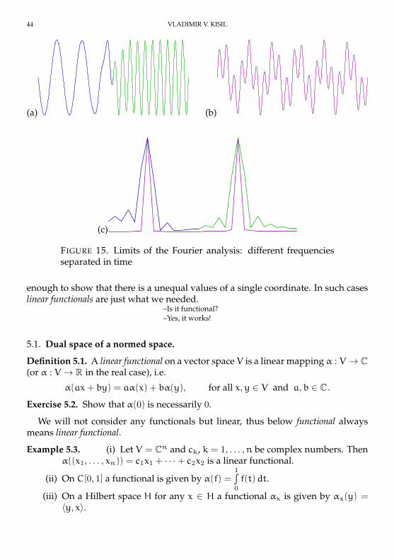
Consider the simple case of the signals plotted on the Figure 15(a) and (b). Theyare both made out of same two pure harmonics:
(i) On the first signal the two harmonics (drawn in blue and green) follow oneafter another in time on Figure 15(a);
(ii) They just blended in equal proportions over the whole interval on Fig-ure 15(b).
This appear to be two very different signals. However the Fourier performedover the whole interval does not seems to be very different, see Figure 15(c). Bothtransforms (drawn in blue-green and pink) have two major pikes corresponding tothe pure frequencies. It is not very easy to extract differences between signals fromtheir Fourier transform (yet this should be possible according to our study).
Even a better picture could be obtained if we use windowed Fourier transform,namely use a sliding “window” of the constant width instead of the entire intervalfor the Fourier transform. Yet even better analysis could be obtained by means ofwavelets already mentioned in Remark 4.12 in connection with Plancherel’s formula.Roughly, wavelets correspond to a sliding window of a variable size—narrow forhigh frequencies and wide for low.
5. DUALITY OF LINEAR SPACES
Everything has another side
Orthonormal basis allows to reduce any question on Hilbert space to a questionon sequence of numbers. This is powerful but sometimes heavy technique. Some-time we need a smaller and faster tool to study questions which are representedby a single number, for example to demonstrate that two vectors are different it is
44 VLADIMIR V. KISIL
(a) (b)
(c)
FIGURE 15. Limits of the Fourier analysis: different frequenciesseparated in time
enough to show that there is a unequal values of a single coordinate. In such caseslinear functionals are just what we needed.
–Is it functional?–Yes, it works!
5.1. Dual space of a normed space.
Definition 5.1. A linear functional on a vector space V is a linear mapping α : V → C(or α : V → R in the real case), i.e.
α(ax+ by) = aα(x) + bα(y), for all x,y ∈ V and a,b ∈ C.
Exercise 5.2. Show that α(0) is necessarily 0.
We will not consider any functionals but linear, thus below functional alwaysmeans linear functional.
Example 5.3. (i) Let V = Cn and ck, k = 1, . . . ,n be complex numbers. Thenα((x1, . . . , xn)) = c1x1 + · · ·+ c2x2 is a linear functional.
(ii) On C[0, 1] a functional is given by α(f) =1∫0
f(t)dt.
(iii) On a Hilbert space H for any x ∈ H a functional αx is given by αx(y) =〈y, x〉.
INTRODUCTION TO FUNCTIONAL ANALYSIS 45
Theorem 5.4. Let V be a normed space and α is a linear functional. The following areequivalent:
(i) α is continuous (at any point of V).(ii) α is continuous at point 0.
(iii) sup|α(x)| : ‖x‖ 6 1 <∞, i.e. α is a bounded linear functional.
Proof. Implication 5.4(i)⇒ 5.4(ii) is trivial.Show 5.4(ii)⇒ 5.4(iii). By the definition of continuity: for any ε > 0 there exists
δ > 0 such that ‖v‖ < δ implies |α(v) − α(0)| < ε. Take ε = 1 then |α(δx)| < 1 forall x with norm less than 1 because ‖δx‖ < δ. But from linearity of α the inequality|α(δx)| < 1 implies |α(x)| < 1/δ <∞ for all ‖x‖ 6 1.
5.4(iii) ⇒ 5.4(i). Let mentioned supremum be M. For any x, y ∈ V such thatx 6= y vector (x − y)/ ‖x− y‖ has norm 1. Thus |α((x− y)/ ‖x− y‖)| < M. By thelinearity of α this implies that |α(x) − α(y)| < M ‖x− y‖. Thus α is continuous.
Definition 5.5. The dual space X∗ of a normed space X is the set of continuous linearfunctionals on X. Define a norm on it by
(5.1) ‖α‖ = sup‖x‖61
|α(x)| .
Exercise 5.6. (i) Show that X∗ is a linear space with natural operations.(ii) Show that (5.1) defines a norm on X∗.
(iii) Show that |α(x)| 6 ‖α‖ · ‖x‖ for all x ∈ X, α ∈ X∗.Theorem 5.7. X∗ is a Banach space with the defined norm (even if X was incomplete).
Proof. Due to Exercise 5.6 we only need to show that X∗ is complete. Let (αn) bea Cauchy sequence in X∗, then for any x ∈ X scalars αn(x) form a Cauchy se-quence, since |αm(x) − αn(x)| 6 ‖αm − αn‖ · ‖x‖. Thus the sequence has a limitand we define α by α(x) = limn→∞ αn(x). Clearly α is a linear functional on X. Weshould show that it is bounded and αn → α. Given ε > 0 there exists N such that‖αn − αm‖ < ε for all n, m > N. If ‖x‖ 6 1 then |αn(x) − αm(x)| 6 ε, let m → ∞then |αn(x) − α(x)| 6 ε, so
|α(x)| 6 |αn(x)|+ ε 6 ‖αn‖+ ε,
i.e. ‖α‖ is finite and ‖αn − α‖ 6 ε, thus αn → α.
Definition 5.8. The kernel of linear functional α, write kerα, is the set all vectors x ∈ Xsuch that α(x) = 0.
Exercise 5.9. Show that(i) kerα is a subspace of X.
(ii) If α 6≡ 0 then kerα is a proper subspace of X.(iii) If α is continuous then kerα is closed.
Study one and get any other for free!Hilbert spaces sale

46 VLADIMIR V. KISIL
5.2. Self-duality of Hilbert space.
Lemma 5.10 (Riesz–Frechet). Let H be a Hilbert space and α a continuous linear func-tional on H, then there exists the unique y ∈ H such that α(x) = 〈x,y〉 for all x ∈ H. Also‖α‖H∗ = ‖y‖H.
Proof. Uniqueness: if 〈x,y〉 = 〈x,y ′〉 ⇔ 〈x,y− y ′〉 = 0 for all x ∈ H then y − y ′ isself-orthogonal and thus is zero (Exercise 3.2(i)).
Existence: we may assume that α 6≡ 0 (otherwise take y = 0), then M = kerα isa closed proper subspace of H. Since H =M⊕M⊥, there exists a non-zero z ∈M⊥,by scaling we could get α(z) = 1. Then for any x ∈ H:
x = (x− α(x)z) + α(x)z, with x− α(x)z ∈M, α(x)z ∈M⊥.
Because 〈x, z〉 = α(x) 〈z, z〉 = α(x) ‖z‖2 for any x ∈ Hwe set y = z/ ‖z‖2.Equality of the norms ‖α‖H∗ = ‖y‖H follows from the Cauchy–Bunyakovskii–
Schwarz inequality in the form α(x) 6 ‖x‖ · ‖y‖ and the identity α(y/ ‖y‖) = ‖y‖.
Example 5.11. On L2[0, 1] let α(f) =⟨f, t2
⟩=
1∫0
f(t)t2 dt. Then
‖α‖ =∥∥t2∥∥ =
1∫0
(t2)2 dt
1/2
=1√5
.
6. OPERATORS
All the space’s a stage,and all functionals and operators merely players!
All our previous considerations were only a preparation of the stage and nowthe main actors come forward to perform a play. The vectors spaces are not sointeresting while we consider them in statics, what really make them exciting is thetheir transformations. The natural first steps is to consider transformations whichrespect both linear structure and the norm.
6.1. Linear operators.
Definition 6.1. A linear operator T between two normed spacesX and Y is a mappingT : X → Y such that T(λv + µu) = λT(v) + µT(u). The kernel of linear operator ker Tand image are defined by
ker T = x ∈ X : Tx = 0 Im T = y ∈ Y : y = Tx, for some x ∈ X.Exercise 6.2. Show that kernel of T is a linear subspace of X and image of T is alinear subspace of Y.
As usual we are interested also in connections with the second (topological)structure:

INTRODUCTION TO FUNCTIONAL ANALYSIS 47
Definition 6.3. A norm of linear operator is defined:
(6.1) ‖T‖ = sup‖Tx‖Y : ‖x‖X 6 1.
T is a bounded linear operator if ‖T‖ = sup‖Tx‖ : ‖x‖ <∞.
Exercise 6.4. Show that ‖Tx‖ 6 ‖T‖ · ‖x‖ for all x ∈ X.
Example 6.5. Consider the following examples and determine kernel and imagesof the mentioned operators.
(i) On a normed space X define the zero operator to a space Y by Z : x → 0 forall x ∈ X. Its norm is 0.
(ii) On a normed space X define the identity operator by IX : x→ x for all x ∈ X.Its norm is 1.
(iii) On a normed space X any linear functional define a linear operator from Xto C, its norm as operator is the same as functional.
(iv) The set of operators from Cn to Cm is given by n × m matrices whichacts on vector by the matrix multiplication. All linear operators on finite-dimensional spaces are bounded.
(v) On `2, let S(x1, x2, . . .) = (0, x1, x2, . . .) be the right shift operator. Clearly‖Sx‖ = ‖x‖ for all x, so ‖S‖ = 1.
(vi) On L2[a,b], let w(t) ∈ C[a,b] and define multiplication operator Mwf by(Mwf)(t) = w(t)f(t). Now:
‖Mwf‖2 =
b∫a
|w(t)|2 |f(t)|2 dt
6 K2
b∫a
|f(t)|2 dt, where K = ‖w‖∞ = sup[a,b]
|w(t)| ,
so ‖Mw‖ 6 K.
Exercise 6.6. Show that for multiplication operator in fact there is the equal-ity of norms ‖Mw‖2 = ‖w(t)‖∞.
Theorem 6.7. Let T : X→ Y be a linear operator. The following conditions are equivalent:(i) T is continuous on X;
(ii) T is continuous at the point 0.(iii) T is a bounded linear operator.
Proof. Proof essentially follows the proof of similar Theorem 5.4.
6.2. B(H) as a Banach space (and even algebra).
Theorem 6.8. Let B(X, Y) be the space of bounded linear operators from X and Y withthe norm defined above. If Y is complete, then B(X, Y) is a Banach space.

48 VLADIMIR V. KISIL
Proof. The proof repeat proof of the Theorem 5.7, which is a particular case of thepresent theorem for Y = C, see Example 6.5(iii).
Theorem 6.9. Let T ∈ B(X, Y) and S ∈ B(Y,Z), where X, Y, and Z are normed spaces.Then ST ∈ B(X,Z) and ‖ST‖ 6 ‖S‖ ‖T‖.Proof. Clearly (ST)x = S(Tx) ∈ Z, and
‖STx‖ 6 ‖S‖ ‖Tx‖ 6 ‖S‖ ‖T‖ ‖x‖ ,
which implies norm estimation if ‖x‖ 6 1.
Corollary 6.10. Let T ∈ B(X,X) =B(X), where X is a normed space. Then for any n > 1,Tn ∈ B(X) and ‖Tn‖ 6 ‖T‖n.
Proof. It is induction by n with the trivial base n = 1 and the step following fromthe previous theorem.
Remark 6.11. Some texts use notations L(X, Y) and L(X) instead of ours B(X, Y) andB(X).
Definition 6.12. Let T ∈ B(X, Y). We say T is an invertible operator if there existsS ∈ B(Y,X) such that
ST = IX and TS = IY .
Such an S is called the inverse operator of T .
Exercise 6.13. Show that(i) for an invertible operator T : X→ Y we have ker T = 0 and =T = Y.
(ii) the inverse operator is unique (if exists at all). (Assume existence of S andS ′, then consider operator STS ′.)
Example 6.14. We consider inverses to operators from Exercise 6.5.(i) The zero operator is never invertible unless the pathological spaces X =Y = 0.
(ii) The identity operator IX is the inverse of itself.(iii) A linear functional is not invertible unless it is non-zero and X is one di-
mensional.(iv) An operator Cn → Cm is invertible if and only ifm = n and corresponding
square matrix is non-singular, i.e. has non-zero determinant.(v) The right shift S is not invertible on `2 (it is one-to-one but is not onto). But
the left shift operator T(x1, x2, . . .) = (x2, x3, . . .) is its left inverse, i.e. TS = Ibut TS 6= I since ST(1, 0, 0, . . .) = (0, 0, . . .). T is not invertible either (it isonto but not one-to-one), however S is its right inverse.
(vi) Operator of multiplication Mw is invertible if and only if w−1 ∈ C[a,b]and inverse is Mw−1 . For example M1+t is invertible L2[0, 1] and Mt isnot.

INTRODUCTION TO FUNCTIONAL ANALYSIS 49
6.3. Adjoints.
Theorem 6.15. LetH andK be Hilbert Spaces and T ∈ B(H,K). Then there exists operatorT∗ ∈ B(K,H) such that
〈Th,k〉K = 〈h, T∗k〉H for all h ∈ H, k ∈ K.
Such T∗ is called the adjoint operator of T . Also T∗∗ = T and ‖T∗‖ = ‖T‖.Proof. For any fixed k ∈ K the expression h :→ 〈Th,k〉K defines a bounded linearfunctional on H. By the Riesz–Frechet lemma there is a unique y ∈ H such that〈Th,k〉K = 〈h,y〉H for all h ∈ H. Define T∗k = y then T∗ is linear:
〈h, T∗(λ1k1 + λ2k2)〉H = 〈Th, λ1k1 + λ2k2〉K= λ1 〈Th,k1〉K + λ2 〈Th,k2〉K= λ1 〈h, T∗k1〉H + λ2 〈h, T∗k2〉K= 〈h, λ1T
∗k1 + λ2T∗k2〉H
So T∗(λ1k1 + λ2k2) = λ1T∗k1 + λ2T
∗k2. T∗∗ is defined by 〈k, T∗∗h〉 = 〈T∗k,h〉 andthe identity 〈T∗∗h,k〉 = 〈h, T∗k〉 = 〈Th,k〉 for all h and k shows T∗∗ = T . Also:
‖T∗k‖2 = 〈T∗k, T∗k〉 = 〈k, TT∗k〉6 ‖k‖ · ‖TT∗k‖ 6 ‖k‖ · ‖T‖ · ‖T∗k‖ ,
which implies ‖T∗k‖ 6 ‖T‖·‖k‖, consequently ‖T∗‖ 6 ‖T‖. The opposite inequalityfollows from the identity ‖T‖ = ‖T∗∗‖.
Exercise 6.16. (i) For operators T1 and T2 show that
(T1T2)∗ = T∗2 T
∗1 , (T1 + T2)
∗ = T∗1 + T∗2 (λT)∗ = λT∗.
(ii) If A is an operator on a Hilbert space H then (kerA)⊥ = ImA∗.
6.4. Hermitian, unitary and normal operators.
Definition 6.17. An operator T : H→ H is a Hermitian operator or self-adjoint operatorif T = T∗, i.e. 〈Tx,y〉 = 〈x, Ty〉 for all x, y ∈ H.
Example 6.18. (i) On `2 the adjoint S∗ to the right shift operator S is given bythe left shift S∗ = T , indeed:
〈Sx,y〉 = 〈(0, x1, x2, . . .), (y1,y2, . . .)〉= x1y2 + x2y3 + · · · = 〈(x1, x2, . . .), (y2,y3, . . .)〉= 〈x, Ty〉 .
Thus S is not Hermitian.(ii) Let D be diagonal operator on `2 given by
D(x1, x2, . . .) = (λ1x1, λ2x2, . . .).

50 VLADIMIR V. KISIL
where (λk) is any bounded complex sequence. It is easy to check that‖D‖ = ‖(λn)‖∞ = supk |λk| and
D∗(x1, x2, . . .) = (λ1x1, λ2x2, . . .),
thus D is Hermitian if and only if λk ∈ R for all k.(iii) If T : Cn → Cn is represented by multiplication of a column vector by a
matrix A, then T∗ is multiplication by the matrix A∗—transpose and con-jugate to A.
Exercise 6.19. Show that for any bounded operator T operators T1 = 12 (T ±T∗), T∗T
and TT∗ are Hermitians.
Theorem 6.20. Let T be a Hermitian operator on a Hilbert space. Then
‖T‖ = sup‖x‖=1
|〈Tx, x〉| .
Proof. If Tx = 0 for all x ∈ H, both sides of the identity are 0. So we suppose that∃x ∈ H for which Tx 6= 0.
We see that |〈Tx, x〉| 6 ‖Tx‖ ‖x‖ 6 ‖T‖∥∥x2∥∥, so sup‖x‖=1 |〈Tx, x〉| 6 ‖T‖. To get
the inequality the other way around, we first write s := sup‖x‖=1 |〈Tx, x〉|. Then forany x ∈ H, we have |〈Tx, x〉| 6 s
∥∥x2∥∥.We now consider
〈T(x+ y), x+ y〉 = 〈Tx, x〉+〈Tx,y〉+〈Ty, x〉+〈Ty,y〉 = 〈Tx, x〉+2< 〈Tx,y〉+〈Ty,y〉(because T being Hermitian gives 〈Ty, x〉 = 〈y, Tx〉 = 〈Tx,y〉) and, similarly,
〈T(x− y), x− y〉 = 〈Tx, x〉− 2< 〈Tx,y〉+ 〈Ty,y〉 .Subtracting gives
4< 〈Tx,y〉 = 〈T(x+ y), x+ y〉− 〈T(x− y), x− y〉6 s(‖x+ y‖2 + ‖x− y‖2)= 2s(‖x‖2 + ‖y‖2),
by the parallelogram identity.Now, for x ∈ H such that Tx 6= 0, we put y = ‖Tx‖−1 ‖x‖ Tx. Then ‖y‖ = ‖x‖
and when we substitute into the previous inequality, we get
4 ‖Tx‖ ‖x‖ = 4< 〈Tx,y〉 6 4s∥∥x2∥∥ ,
So ‖Tx‖ 6 s ‖x‖ and it follows that ‖T‖ 6 s, as required.
Definition 6.21. We say that U : H→ H is a unitary operator on a Hilbert space H ifU∗ = U−1, i.e. U∗U = UU∗ = I.
Example 6.22. (i) If D : `2 → `2 is a diagonal operator such that Dek = λkek,then D∗ek = λkek and D is unitary if and only if |λk| = 1 for all k.
(ii) The shift operator S satisfies S∗S = I but SS∗ 6= I thus S is not unitary.

INTRODUCTION TO FUNCTIONAL ANALYSIS 51
Theorem 6.23. For an operator U on a complex Hilbert space H the following are equival-ent:
(i) U is unitary;(ii) U is surjection and an isometry, i.e. ‖Ux‖ = ‖x‖ for all x ∈ H;
(iii) U is a surjection and preserves the inner product, i.e. 〈Ux,Uy〉 = 〈x,y〉 for all x,y ∈ H.
Proof. 6.23(i)⇒6.23(ii). Clearly unitarity of operator implies its invertibility andhence surjectivity. Also
‖Ux‖2 = 〈Ux,Ux〉 = 〈x,U∗Ux〉 = 〈x, x〉 = ‖x‖2 .
6.23(ii)⇒6.23(iii). Using the polarisation identity (cf. polarisation in equation (2.6)):
4 〈Tx,y〉 = 〈T(x+ y), x+ y〉+ i 〈T(x+ iy), x+ iy〉− 〈T(x− y), x− y〉− i 〈T(x− iy), x− iy〉 .
=
3∑k=0
ik⟨T(x+ iky), x+ iky
⟩Take T = U∗U and T = I, then
4 〈U∗Ux,y〉 =
3∑k=0
ik⟨U∗U(x+ iky), x+ iky
⟩=
3∑k=0
ik⟨U(x+ iky),U(x+ iky)
⟩=
3∑k=0
ik⟨(x+ iky), (x+ iky)
⟩= 4 〈x,y〉 .
6.23(iii)⇒6.23(i). Indeed 〈U∗Ux,y〉 = 〈x,y〉 implies 〈(U∗U− I)x,y〉 = 0 for all x,y ∈H, then U∗U = I. Since U should be invertible by surjectivity we see that U∗ =U−1.
Definition 6.24. A normal operator T is one for which T∗T = TT∗.
Example 6.25. (i) Any self-adjoint operator T is normal, since T∗ = T .(ii) Any unitary operator U is normal, since U∗U = I = UU∗.
(iii) Any diagonal operator D is normal , since Dek = λkek, D∗ek = λkek, andDD∗ek = D∗Dek = |λk|
2 ek.(iv) The shift operator S is not normal.(v) A finite matrix is normal (as an operator on `n2 ) if and only if it has an
orthonormal basis in which it is diagonal.

52 VLADIMIR V. KISIL
Remark 6.26. Theorems 6.20 and 6.23(ii) draw similarity between those types ofoperators and multiplications by complex numbers. Indeed Theorem 6.20 said thatan operator which significantly change direction of vectors (“rotates”) cannot beHermitian, just like a multiplication by a real number scales but do not rotate. Onthe other hand Theorem 6.23(ii) says that unitary operator just rotate vectors butdo not scale, as a multiplication by an unimodular complex number. We will seefurther such connections in Theorem 7.17.
7. SPECTRAL THEORY
Beware of ghosts2 in this area!
As we saw operators could be added and multiplied each other, in some sensethey behave like numbers, but are much more complicated. In this lecture we willassociate to each operator a set of complex numbers which reflects certain (unfor-tunately not all) properties of this operator.
The analogy between operators and numbers become even more deeper sincewe could construct functions of operators (called functional calculus) in a way we buildnumeric functions. The most important functions of this sort is called resolvent (seeDefinition 7.5). The methods of analytical functions are very powerful in operatortheory and students may wish to refresh their knowledge of complex analysis be-fore this part.
7.1. The spectrum of an operator on a Hilbert space. An eigenvalue of operatorT ∈ B(H) is a complex number λ such that there exists a nonzero x ∈ H, calledeigenvector with property Tx = λx, in other words x ∈ ker(T − λI).
In finite dimensions T − λI is invertible if and only if λ is not an eigenvalue. Ininfinite dimensions it is not the same: the right shift operator S is not invertible but0 is not its eigenvalue because Sx = 0 implies x = 0 (check!).
Definition 7.1. The resolvent set ρ(T) of an operator T is the set
ρ(T) = λ ∈ C : T − λI is invertible.
The spectrum of operator T ∈ B(H), denoted σ(T), is the complement of the resolventset ρ(T):
σ(T) = λ ∈ C : T − λI is not invertible.
Example 7.2. If H is finite dimensional the from previous discussion follows thatσ(T) is the set of eigenvalues of T for any T .
Even this example demonstrates that spectrum does not provide a complete de-scription for operator even in finite-dimensional case. For example, both operators
in C2 given by matrices(
0 00 0
)and
(0 01 0
)have a single point spectrum 0,
however are rather different. The situation became even worst in the infinite di-mensional spaces.

INTRODUCTION TO FUNCTIONAL ANALYSIS 53
Theorem 7.3. The spectrum σ(T) of a bounded operator T is a nonempty compact (i.e.closed and bounded) subset of C.
For the proof we will need several Lemmas.
Lemma 7.4. Let A ∈ B(H). If ‖A‖ < 1 then I − A is invertible in B(H) and inverse isgiven by the Neumann series (C. Neumann, 1877):
(7.1) (I−A)−1 = I+A+A2 +A3 + . . . =
∞∑k=0
Ak.
Proof. Define the sequence of operators Bn = I+A+ · · ·+AN—the partial sums ofthe infinite series (7.1). It is a Cauchy sequence, indeed:
‖Bn − Bm‖ =∥∥Am+1 +Am+2 + · · ·+An
∥∥ (if n < m)
6∥∥Am+1
∥∥+ ∥∥Am+2∥∥+ · · ·+ ‖An‖
6 ‖A‖m+1 + ‖A‖m+2 + · · ·+ ‖A‖n
6‖A‖m+1
1 − ‖A‖ < ε
for a large m. By the completeness of B(H) there is a limit, say B, of the sequenceBn. It is a simple algebra to check that (I−A)Bn = Bn(I−A) = I−A
n+1, passingto the limit in the norm topology, where An+1 → 0 and Bn → Bwe get:
(I−A)B = B(I−A) = I ⇔ B = (I−A)−1.
Definition 7.5. The resolventof an operator T is the operator valued function definedon the resolvent set by the formula:
(7.2) R(λ, T) = (T − λI)−1.
Corollary 7.6. (i) If |λ| > ‖T‖ then λ ∈ ρ(T), hence the spectrum is bounded.(ii) The resolvent set ρ(T) is open, i.e for any λ ∈ ρ(T) then there exist ε > 0 such
that all µ with |λ− µ| < ε are also in ρ(T), i.e. the resolvent set is open and thespectrum is closed.
Both statements together imply that the spectrum is compact.
Proof. (i) If |λ| > ‖T‖ then∥∥λ−1T
∥∥ < 1 and the operator T −λI = −λ(I−λ−1T)has the inverse
(7.3) R(λ, T) = (T − λI)−1 = −
∞∑k=0
λ−k−1Tk.
by the previous Lemma.
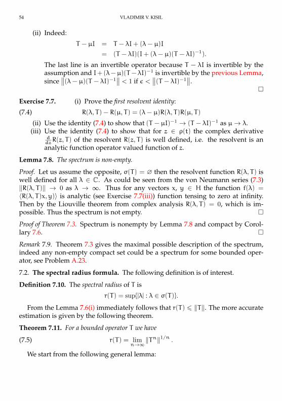
54 VLADIMIR V. KISIL
(ii) Indeed:
T − µI = T − λI+ (λ− µ)I
= (T − λI)(I+ (λ− µ)(T − λI)−1).
The last line is an invertible operator because T − λI is invertible by theassumption and I+(λ−µ)(T − λI)−1 is invertible by the previous Lemma,since
∥∥(λ− µ)(T − λI)−1∥∥ < 1 if ε <
∥∥(T − λI)−1∥∥.
Exercise 7.7. (i) Prove the first resolvent identity:
(7.4) R(λ, T) − R(µ, T) = (λ− µ)R(λ, T)R(µ, T)
(ii) Use the identity (7.4) to show that (T − µI)−1 → (T − λI)−1 as µ→ λ.(iii) Use the identity (7.4) to show that for z ∈ ρ(t) the complex derivative
ddzR(z, T) of the resolvent R(z, T) is well defined, i.e. the resolvent is an
analytic function operator valued function of z.
Lemma 7.8. The spectrum is non-empty.
Proof. Let us assume the opposite, σ(T) = ∅ then the resolvent function R(λ, T) iswell defined for all λ ∈ C. As could be seen from the von Neumann series (7.3)‖R(λ, T)‖ → 0 as λ → ∞. Thus for any vectors x, y ∈ H the function f(λ) =〈R(λ, T)x,y)〉 is analytic (see Exercise 7.7(iii)) function tensing to zero at infinity.Then by the Liouville theorem from complex analysis R(λ, T) = 0, which is im-possible. Thus the spectrum is not empty.
Proof of Theorem 7.3. Spectrum is nonempty by Lemma 7.8 and compact by Corol-lary 7.6.
Remark 7.9. Theorem 7.3 gives the maximal possible description of the spectrum,indeed any non-empty compact set could be a spectrum for some bounded oper-ator, see Problem A.23.
7.2. The spectral radius formula. The following definition is of interest.
Definition 7.10. The spectral radius of T is
r(T) = sup|λ| : λ ∈ σ(T).From the Lemma 7.6(i) immediately follows that r(T) 6 ‖T‖. The more accurate
estimation is given by the following theorem.
Theorem 7.11. For a bounded operator T we have
(7.5) r(T) = limn→∞ ‖Tn‖1/n .
We start from the following general lemma:

INTRODUCTION TO FUNCTIONAL ANALYSIS 55
Lemma 7.12. Let a sequence (an) of positive real numbers satisfies inequalities: 0 6am+n 6 am + an for all m and n. Then there is a limit lim
n→∞(an/n) and its equal toinfn(an/n).
Proof. The statements follows from the observation that for any n and m = nk + lwith 0 6 l 6 n we have am 6 kan + la1 thus, for big m we got am/m 6 an/n +la1/m 6 an/n+ ε.
Proof of Theorem 7.11. The existence of the limit limn→∞ ‖Tn‖1/n in (7.5) followsfrom the previous Lemma since by the Lemma 6.9 log ‖Tn+m‖ 6 log ‖Tn‖+log ‖Tm‖.Now we are using some results from the complex analysis. The Laurent series forthe resolvent R(λ, T) in the neighbourhood of infinity is given by the von Neumannseries (7.3). The radius of its convergence (which is equal, obviously, to r(T)) by theHadamard theorem is exactly limn→∞ ‖Tn‖1/n.
Corollary 7.13. There exists λ ∈ σ(T) such that |λ| = r(T).
Proof. Indeed, as its known from the complex analysis the boundary of the con-vergence circle of a Laurent (or Taylor) series contain a singular point, the singularpoint of the resolvent is obviously belongs to the spectrum.
Example 7.14. Let us consider the left shift operator S∗, for any λ ∈ C such that|λ| < 1 the vector (1, λ, λ2, λ3, . . .) is in `2 and is an eigenvector of S∗ with eigenvalueλ, so the open unit disk |λ| < 1 belongs to σ(S∗). On the other hand spectrum of S∗
belongs to the closed unit disk |λ| 6 1 since r(S∗) 6 ‖S∗‖ = 1. Because spectrum isclosed it should coincide with the closed unit disk, since the open unit disk is densein it. Particularly 1 ∈ σ(S∗), but it is easy to see that 1 is not an eigenvalue of S∗.
Proposition 7.15. For any T ∈ B(H) the spectrum of the adjoint operator is σ(T∗) = λ :λ ∈ σ(T).Proof. If (T−λI)V = V(T−λI) = I the by taking adjoints V∗(T∗−λI) = (T∗−λI)V∗ =I. So λ ∈ ρ(T) implies λ ∈ ρ(T∗), using the property T∗∗ = T we could invert theimplication and get the statement of proposition.
Example 7.16. In continuation of Example 7.14 using the previous Proposition weconclude that σ(S) is also the closed unit disk, but S does not have eigenvalues atall!
7.3. Spectrum of Special Operators.
Theorem 7.17. (i) If U is a unitary operator then σ(U) ⊆ |z| = 1.(ii) If T is Hermitian then σ(T) ⊆ R.
Proof. (i) If |λ| > 1 then∥∥λ−1U
∥∥ < 1 and then λI−U = λ(I−λ−1U) is invertible,thus λ 6∈ σ(U). If |λ| < 1 then ‖λU∗‖ < 1 and then λI − U = U(λU∗ − I) isinvertible, thus λ 6∈ σ(U). The remaining set is exactly z : |z| = 1.

56 VLADIMIR V. KISIL
(ii) Without lost of generality we could assume that ‖T‖ < 1, otherwise wecould multiply T by a small real scalar. Let us consider the Cayley transformwhich maps real axis to the unit circle:
U = (T − iI)(T + iI)−1.
Straightforward calculations show that U is unitary if T is Hermitian. Letus take λ 6∈ R and λ 6= −i (this case could be checked directly by Lemma 7.4).Then the Cayley transform µ = (λ− i)(λ+ i)−1 of λ is not on the unit circleand thus the operator
U− µI = (T − iI)(T + iI)−1 − (λ− i)(λ+ i)−1I = 2i(λ+ i)−1(T − λI)(T + iI)−1,
is invertible, which implies invertibility of T − λI. So λ 6∈ R.
The above reduction of a self-adjoint operator to a unitary one (it can be done onthe opposite direction as well!) is an important tool which can be applied in otherquestions as well, e.g. in the following exercise.
Exercise 7.18. (i) Show that an operator U : f(t) 7→ eitf(t) on L2[0, 2π] is unit-ary and has the entire unit circle |z| = 1 as its spectrum .
(ii) Find a self-adjoint operator T with the entire real line as its spectrum.
8. COMPACTNESS
It is not easy to study linear operators “in general” and there are many ques-tions about operators in Hilbert spaces raised many decades ago which are stillunanswered. Therefore it is reasonable to single out classes of operators whichhave (relatively) simple properties. Such a class of operators more closed to finitedimensional ones will be studied here.
These operators are so compact that we even can fit them inour course
8.1. Compact operators. Let us recall some topological definition and results.
Definition 8.1. A compact set in a metric space is defined by the property that anyits covering by a family of open sets contains a subcovering by a finite subfamily.
In the finite dimensional vector spaces Rn or Cn there is the following equivalentdefinition of compactness (equivalence of 8.2(i) and 8.2(ii) is known as Heine–Boreltheorem):
Theorem 8.2. If a set E in Rn or Cn has any of the following properties then it has othertwo as well:
(i) E is bounded and closed;(ii) E is compact;
(iii) Any infinite subset of E has a limiting point belonging to E.

INTRODUCTION TO FUNCTIONAL ANALYSIS 57
Exercise∗ 8.3. Which equivalences from above are not true any more in the infinitedimensional spaces?
Definition 8.4. Let X and Y be normed spaces, T ∈ B(X, Y) is a finite rank operator ifIm T is a finite dimensional subspace of Y. T is a compact operator if whenever (xi)∞1is a bounded sequence in X then its image (Txi)
∞1 has a convergent subsequence in
Y.The set of finite rank operators is denote by F(X, Y) and the set of compact
operators—by K(X, Y)
Exercise 8.5. Show that both F(X, Y) and K(X, Y) are linear subspaces of B(X, Y).
We intend to show that F(X, Y) ⊂ K(X, Y).
Lemma 8.6. Let Z be a finite-dimensional normed space. Then there is a number N and amapping S : `N2 → Z which is invertible and such that S and S−1 are bounded.
Proof. The proof is given by an explicit construction. Let N = dimZ and z1, z2, . . . ,zN be a basis in Z. Let us define
S : `N2 → Z by S(a1,a2, . . . ,aN) =
N∑k=1
akzk,
then we have an estimation of norm:
‖Sa‖ =
∥∥∥∥∥N∑k=1
akzk
∥∥∥∥∥ 6N∑k=1
|ak| ‖zk‖
6
(N∑k=1
|ak|2
)1/2( N∑k=1
‖zk‖2)1/2
.
So ‖S‖ 6(∑N
1 ‖zk‖2)1/2
and S is continuous.Clearly S has the trivial kernel, particularly ‖Sa‖ > 0 if ‖a‖ = 1. By the Heine–
Borel theorem the unit sphere in `N2 is compact, consequently the continuous func-tion a 7→
∥∥∥∑N1 akzk
∥∥∥ attains its lower bound, which has to be positive. This meansthere exists δ > 0 such that ‖a‖ = 1 implies ‖Sa‖ > δ, or, equivalently if ‖z‖ < δ
then∥∥S−1z
∥∥ < 1. The later means that∥∥S−1
∥∥ 6 δ−1 and boundedness of S−1.
Corollary 8.7. For any two metric spaces X and Y we have F(X, Y) ⊂ K(X, Y).
Proof. Let T ∈ F(X, Y), if (xn)∞1 is a bounded sequence in X then ((Txn)∞1 ⊂ Z =
Im T is also bounded. Let S : `N2 → Z be a map constructed in the above Lemma.The sequence (S−1Txn)
∞1 is bounded in `N2 and thus has a limiting point, say a0.
Then Sa0 is a limiting point of (Txn)∞1 .
There is a simple condition which allows to determine which diagonal operatorsare compact (particularly the identity operator IXis not compact if dimX =∞):

58 VLADIMIR V. KISIL
Proposition 8.8. Let T is a diagonal operator and given by identities Ten = λnen for alln in a basis en. T is compact if and only if λn → 0.
Proof. If λn 6→ 0 then there exists a subsequence λnkand δ > 0 such that |λnk
| > δfor all k. Now the sequence (enk
) is bounded but its image Tenk= λnk
enkhas no
convergent subsequence because for any k 6= l:‖λnk
enk− λnl
enl‖ = (|λnk
|2 + |λnl
|2)1/2 >
√2δ,
i.e. Tenkis not a Cauchy sequence, see Figure 16.
e1λ1e1
δe1
e2
λ2e2
δe2
FIGURE 16. Distance between scales of orthonormal vectors
For the converse, note that if λn → 0 then we can define a finite rank operatorTm,m > 1—m-“truncation” of T by:
(8.1) Tmen =
Ten = λnen, 1 6 n 6 m;0, n > m.
Then obviously
(T − Tm)en =
0, 1 6 n 6 m;λnen, n > m,
and ‖T − Tm‖ = supn>m |λn| → 0 if m → ∞. All Tm are finite rank operators (soare compact) and T is also compact as their limit—by the next Theorem.
Theorem 8.9. Let Tm be a sequence of compact operators convergent to an operator T inthe norm topology (i.e. ‖T − Tm‖ → 0) then T is compact itself. Equivalently K(X, Y) is aclosed subspace of B(X, Y).
Proof. Take a bounded sequence (xn)∞1 . From compactness
of T1 ⇒ ∃ subsequence (x(1)n )∞1 of (xn)∞1 s.t. (T1x
(1)n )∞1 is convergent.
of T2 ⇒ ∃ subsequence (x(2)n )∞1 of (x(1)n )∞1 s.t. (T2x
(2)n )∞1 is convergent.
of T3 ⇒ ∃ subsequence (x(3)n )∞1 of (x(2)n )∞1 s.t. (T3x
(3)n )∞1 is convergent.
. . . . . . . . . . . . . . .Could we find a subsequence which converges for all Tm simultaneously? The firstguess “take the intersection of all above sequences (x(k)n )∞1 ” does not work because

INTRODUCTION TO FUNCTIONAL ANALYSIS 59
the intersection could be empty. The way out is provided by the diagonal argument(see Table 2): a subsequence (Tmx
(k)k )∞1 is convergent for all m, because at latest
after the term x(m)m it is a subsequence of (x(m)
k )∞1 .
T1x(1)1 T1x
(1)2 T1x
(1)3 . . . T1x
(1)n . . . → a1
T2x(2)1 T2x
(2)2 T2x
(2)3 . . . T2x
(2)n . . . → a2
T3x(3)1 T3x
(3)2 T3x
(3)3 . . . T3x
(3)n . . . → a3
. . . . . . . . . . . . . . . . . .Tnx
(n)1 Tnx
(n)2 Tnx
(n)3 . . . Tnx
(n)n . . . → an
. . . . . . . . . . . . . . . . . . ↓
aTABLE 2. The “diagonal argument”.
We are claiming that a subsequence (Tx(k)k )∞1 of (Txn)∞1 is convergent as well.
We use here ε/3 argument (see Figure 17): for a given ε > 0 choose p ∈ N such that‖T − Tp‖ < ε/3. Because (Tpx
(k)k ) → 0 it is a Cauchy sequence, thus there exists
|f(x)− fn(x)| < ǫ/3
|fn(x)− fn(y)| < ǫ/3
|fn(y)− f(y)| < ǫ/3
x y
fn(t)
f(t)
FIGURE 17. The ε/3 argument to estimate |f(x) − f(y)|.
n0 > p such that∥∥∥Tpx(k)k − Tpx
(l)l
∥∥∥ < ε/3 for all k, l > n0. Then:∥∥∥Tx(k)k − Tx(l)l
∥∥∥ =∥∥∥(Tx(k)k − Tpx
(k)k ) + (Tpx
(k)k − Tpx
(l)l ) + (Tpx
(l)l − Tx
(l)l )∥∥∥
6∥∥∥Tx(k)k − Tpx
(k)k
∥∥∥+ ∥∥∥Tpx(k)k − Tpx(l)l
∥∥∥+ ∥∥∥Tpx(l)l − Tx(l)l
∥∥∥6 ε

60 VLADIMIR V. KISIL
Thus T is compact.
8.2. Hilbert–Schmidt operators.
Definition 8.10. Let T : H → K be a bounded linear map between two Hilbertspaces. Then T is said to be Hilbert–Schmidt operator if there exists an orthonormalbasis in H such that the series
∑∞k=1 ‖Tek‖2 is convergent.
Example 8.11. (i) Let T : `2 → `2 be a diagonal operator defined by Ten =
en/n, for all n > 1. Then∑ ‖Ten‖2 =
∑n−2 = π2/6 (see Example 4.14) is
finite.(ii) The identity operator IH is not a Hilbert–Schmidt operator, unless H is
finite dimensional.
A relation to compact operator is as follows.
Theorem 8.12. All Hilbert–Schmidt operators are compact. (The opposite inclusion isfalse, give a counterexample!)
Proof. Let T ∈ B(H,K) have a convergent series∑ ‖Ten‖2 in an orthonormal basis
(en)∞1 of H. We again (see (8.1)) define them-truncation of T by the formula
(8.2) Tmen =
Ten, 1 6 n 6 m;0, n > m.
Then Tm(∑∞
1 akek) =∑m
1 akek and each Tm is a finite rank operator because itsimage is spanned by the finite set of vectors Te1, . . . , Ten. We claim that ‖T − Tm‖ →0. Indeed by linearity and definition of Tm:
(T − Tm)
( ∞∑n=1
anen
)=
∞∑n=m+1
an(Ten).
Thus:∥∥∥∥∥(T − Tm)
( ∞∑n=1
anen
)∥∥∥∥∥ =
∥∥∥∥∥∞∑
n=m+1
an(Ten)
∥∥∥∥∥(8.3)
6∞∑
n=m+1
|an| ‖(Ten)‖
6
( ∞∑n=m+1
|an|2
)1/2( ∞∑n=m+1
‖(Ten)‖2)1/2
6
∥∥∥∥∥∞∑n=1
anen
∥∥∥∥∥( ∞∑n=m+1
‖(Ten)‖2)1/2
(8.4)
so ‖T − Tm‖ → 0 and by the previous Theorem T is compact as a limit of compactoperators.

INTRODUCTION TO FUNCTIONAL ANALYSIS 61
Corollary 8.13 (from the above proof). For a Hilbert–Schmidt operator
‖T‖ 6( ∞∑n=m+1
‖(Ten)‖2)1/2
.
Proof. Just consider difference of T and T0 = 0 in (8.3)–(8.4).
Example 8.14. An integral operator T on L2[0, 1] is defined by the formula:
(8.5) (Tf)(x) =
1∫0
K(x,y)f(y)dy, f(y) ∈ L2[0, 1],
where the continuous on [0, 1] × [0, 1] function K is called the kernel of integral oper-ator.
Theorem 8.15. Integral operator (8.5) is Hilbert–Schmidt.
Proof. Let (en)∞−∞ be an orthonormal basis of L2[0, 1], e.g. (e2πint)n∈Z . Let us con-sider the kernel Kx(y) = K(x,y) as a function of the argument y depending fromthe parameter x. Then:
(Ten)(x) =
1∫0
K(x,y)en(y)dy =
1∫0
Kx(y)en(y)dy = 〈Kx, en〉 .
So ‖Ten‖2 =1∫0
|〈Kx, en〉|2 dx. Consequently:
∞∑−∞ ‖Ten‖
2 =
∞∑−∞
1∫0
|〈Kx, en〉|2 dx
=
1∫0
∞∑1
|〈Kx, en〉|2 dx(8.6)
=
1∫0
‖Kx‖2 dx
=
1∫0
1∫0
|K(x,y)|2 dxdy <∞Exercise 8.16. Justify the exchange of summation and integration in (8.6).
Remark 8.17. The definition 8.14 and Theorem 8.15 work also for any T : L2[a,b]→L2[c,d] with a continuous kernel K(x,y) on [c,d]× [a,b].

62 VLADIMIR V. KISIL
Definition 8.18. Define Hilbert–Schmidt norm of a Hilbert–Schmidt operator A by‖A‖2HS =
∑∞n=1 ‖Aen‖2 (it is independent of the choice of orthonormal basis (en)∞1 ,
see Question A.27).
Exercise∗ 8.19. Show that set of Hilbert–Schmidt operators with the above norm isa Hilbert space and find the an expression for the inner product.
Example 8.20. Let K(x,y) = x− y, then
(Tf)(x) =
1∫0
(x− y)f(y)dy = x
1∫0
f(y)dy−
1∫0
yf(y)dy
is a rank 2 operator. Furthermore:
‖T‖2HS =
1∫0
1∫0
(x− y)2 dxdy =
1∫0
[(x− y)3
3
]1x=0
dy
=
1∫0
(1 − y)3
3+y3
3dy =
[−(1 − y)4
12+y4
12
]10
=1
6.
On the other hand there is an orthonormal basis such that
Tf =1√12〈f, e1〉 e1 −
1√12〈f, e2〉 e2,
and ‖T‖ = 1√12
and∑2
1 ‖Tek‖2 = 16 and we get ‖T‖ 6 ‖T‖HS in agreement with
Corollary 8.13.
9. THE SPECTRAL THEOREM FOR COMPACT NORMAL OPERATORS
Recall from Section 6.4 that an operator T is normal if TT∗ = T∗T ; Hermitian(T∗ = T ) and unitary (T∗ = T−1) operators are normal.
9.1. Spectrum of normal operators.
Theorem 9.1. Let T ∈ B(H) be a normal operator then(i) ker T = ker T∗, so ker(T − λI) = ker(T∗ − λI) for all λ ∈ C
(ii) Eigenvectors corresponding to distinct eigenvalues are orthogonal.(iii) ‖T‖ = r(T).
Proof. (i) Obviously:
x ∈ ker T ⇔ 〈Tx, Tx〉 = 0⇔ 〈T∗Tx, x〉 = 0
⇔ 〈TT∗x, x〉 = 0⇔ 〈T∗x, T∗x〉 = 0
⇔ x ∈ ker T∗.
The second part holds because normalities of T and T − λI are equivalent.

INTRODUCTION TO FUNCTIONAL ANALYSIS 63
(ii) If Tx = λx, Ty = µy then from the previous statement T∗y = µy. If λ 6= µthen the identity
λ 〈x,y〉 = 〈Tx,y〉 = 〈x, T∗y〉 = µ 〈x,y〉implies 〈x,y〉 = 0.
(iii) Let S = T∗T then normality of T implies that S is Hermitian (check!). Con-sequently inequality
‖Sx‖2 = 〈Sx,Sx〉 =⟨S2x, x
⟩6∥∥S2∥∥ ‖x‖2
implies ‖S‖2 6∥∥S2∥∥. But the opposite inequality follows from the The-
orem 6.9, thus we have the equality∥∥S2∥∥ = ‖S‖2 and more generally by
induction:∥∥S2m∥∥ = ‖S‖2m for allm.
Now we claim ‖S‖ = ‖T‖2. From Theorem 6.9 and 6.15 we get ‖S‖ =
‖T∗T‖ 6 ‖T‖2. On the other hand if ‖x‖ = 1 then
‖T∗T‖ > |〈T∗Tx, x〉| = 〈Tx, Tx〉 = ‖Tx‖2
implies the opposite inequality ‖S‖ > ‖T‖2. And because (T2m
)∗T2m
=(T∗T)2
m
we get the equality∥∥T2m∥∥2 =∥∥(T∗T)2m∥∥ = ‖T∗T‖2m = ‖T‖2m+1
.
Thus:
r(T) = limm→∞
∥∥T2m∥∥1/2m = limm→∞ ‖T‖2
m+1/2m+1
= ‖T‖ .
by the spectral radius formula (7.5).
Example 9.2. It is easy to see that normality is important in 9.1(iii), indeed the non-
normal operator T given by the matrix(
0 10 0
)in C has one-point spectrum 0,
consequently r(T) = 0 but ‖T‖ = 1.
Lemma 9.3. Let T be a compact normal operator then(i) The set of of eigenvalues of T is either finite or a countable sequence tending to
zero.(ii) All the eigenspaces, i.e. ker(T − λI), are finite-dimensional for all λ 6= 0.
Remark 9.4. This Lemma is true for any compact operator, but we will not use thatin our course.
Proof. (i) Let H0 be the closed linear span of eigenvectors of T . Then T restric-ted to H0 is a diagonal compact operator with the same set of eigenvaluesλn as in H. Then λn → 0 from Proposition 8.8 .
Exercise 9.5. Use the proof of Proposition 8.8 to give a direct demonstra-tion.
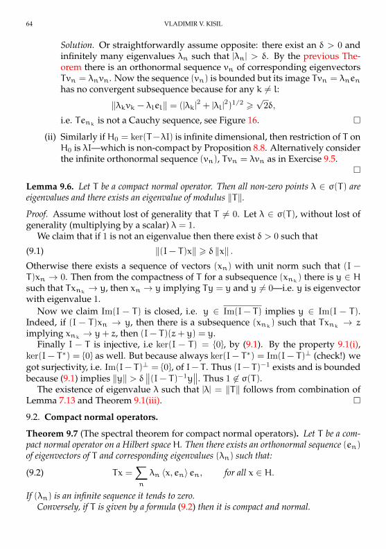
64 VLADIMIR V. KISIL
Solution. Or straightforwardly assume opposite: there exist an δ > 0 andinfinitely many eigenvalues λn such that |λn| > δ. By the previous The-orem there is an orthonormal sequence vn of corresponding eigenvectorsTvn = λnvn. Now the sequence (vn) is bounded but its image Tvn = λnenhas no convergent subsequence because for any k 6= l:
‖λkvk − λlel‖ = (|λk|2 + |λl|
2)1/2 >√
2δ,
i.e. Tenkis not a Cauchy sequence, see Figure 16.
(ii) Similarly ifH0 = ker(T−λI) is infinite dimensional, then restriction of T onH0 is λI—which is non-compact by Proposition 8.8. Alternatively considerthe infinite orthonormal sequence (vn), Tvn = λvn as in Exercise 9.5.
Lemma 9.6. Let T be a compact normal operator. Then all non-zero points λ ∈ σ(T) areeigenvalues and there exists an eigenvalue of modulus ‖T‖.Proof. Assume without lost of generality that T 6= 0. Let λ ∈ σ(T), without lost ofgenerality (multiplying by a scalar) λ = 1.
We claim that if 1 is not an eigenvalue then there exist δ > 0 such that
(9.1) ‖(I− T)x‖ > δ ‖x‖ .
Otherwise there exists a sequence of vectors (xn) with unit norm such that (I −T)xn → 0. Then from the compactness of T for a subsequence (xnk
) there is y ∈ Hsuch that Txnk
→ y, then xn → y implying Ty = y and y 6= 0—i.e. y is eigenvectorwith eigenvalue 1.
Now we claim Im(I − T) is closed, i.e. y ∈ Im(I− T) implies y ∈ Im(I − T).Indeed, if (I − T)xn → y, then there is a subsequence (xnk
) such that Txnk→ z
implying xnk→ y+ z, then (I− T)(z+ y) = y.
Finally I − T is injective, i.e ker(I − T) = 0, by (9.1). By the property 9.1(i),ker(I − T∗) = 0 as well. But because always ker(I − T∗) = Im(I − T)⊥ (check!) wegot surjectivity, i.e. Im(I− T)⊥ = 0, of I− T . Thus (I− T)−1 exists and is boundedbecause (9.1) implies ‖y‖ > δ
∥∥(I− T)−1y∥∥. Thus 1 6∈ σ(T).
The existence of eigenvalue λ such that |λ| = ‖T‖ follows from combination ofLemma 7.13 and Theorem 9.1(iii).
9.2. Compact normal operators.
Theorem 9.7 (The spectral theorem for compact normal operators). Let T be a com-pact normal operator on a Hilbert spaceH. Then there exists an orthonormal sequence (en)of eigenvectors of T and corresponding eigenvalues (λn) such that:
(9.2) Tx =∑n
λn 〈x, en〉 en, for all x ∈ H.
If (λn) is an infinite sequence it tends to zero.Conversely, if T is given by a formula (9.2) then it is compact and normal.

INTRODUCTION TO FUNCTIONAL ANALYSIS 65
Proof. Suppose T 6= 0. Then by the previous Theorem there exists an eigenvalueλ1 such that |λ1| = ‖T‖ with corresponding eigenvector e1 of the unit norm. LetH1 = Lin(e1)
⊥. If x ∈ H1 then
(9.3) 〈Tx, e1〉 = 〈x, T∗e1〉 =⟨x, λ1e1
⟩= λ1 〈x, e1〉 = 0,
thus Tx ∈ H1 and similarly T∗x ∈ H1. Write T1 = T |H1which is again a normal
compact operator with a norm does not exceeding ‖T‖. We could inductively repeatthis procedure for T1 obtaining sequence of eigenvalues λ2, λ3, . . . with eigenvectorse2, e3, . . . . If Tn = 0 for a finite n then theorem is already proved. Otherwise wehave an infinite sequence λn → 0. Let
x =
n∑1
〈x, ek〉 ek + yn ⇒ ‖x‖2 =
n∑1
|〈x, ek〉|2 + ‖yn‖2 , yn ∈ Hn,
from Pythagoras’s theorem. Then ‖yn‖ 6 ‖x‖ and ‖Tyn‖ 6 ‖Tn‖ ‖yn‖ 6 |λn| ‖x‖ →0 by Lemma 9.3. Thus
Tx = limn→∞
(n∑1
〈x, en〉 Ten + Tyn
)=
∞∑1
λn 〈x, en〉 en
Conversely, if Tx =∑∞
1 λn 〈x, en〉 en then
〈Tx,y〉 =∞∑1
λn 〈x, en〉 〈en,y〉 =∞∑1
〈x, en〉 λn〈y, en〉,
thus T∗y =∑∞
1 λn 〈y, en〉 en. Then we got the normality of T : T∗Tx = TT∗x =∑∞1 |λn|
2 〈y, en〉 en. Also T is compact because it is a uniform limit of the finiterank operators Tnx =
∑n1 λn 〈x, en〉 en.
Corollary 9.8. Let T be a compact normal operator on a separable Hilbert space H, thenthere exists a orthonormal basis gk such that
Tx =
∞∑1
λn 〈x,gn〉gn,
and λn are eigenvalues of T including zeros.
Proof. Let (en) be the orthonormal sequence constructed in the proof of the previ-ous Theorem. Then x is perpendicular to all en if and only if its in the kernel of T .Let (fn) be any orthonormal basis of ker T . Then the union of (en) and (fn) is theorthonormal basis (gn) we have looked for.
Exercise 9.9. Finish all details in the above proof.
Corollary 9.10 (Singular value decomposition). If T is any compact operator on aseparable Hilbert space then there exists orthonormal sequences (ek) and (fk) such thatTx =
∑k µk 〈x, ek〉 fk where (µk) is a sequence of positive numbers such that µk → 0 if
it is an infinite sequence.

66 VLADIMIR V. KISIL
Proof. Operator T∗T is compact and Hermitian (hence normal). From the previousCorollary there is an orthonormal basis (ek) such that T∗Tx =
∑n λn 〈x, ek〉 ek for
some positive λn = ‖Ten‖2. Let µn = ‖Ten‖ and fn = Ten/µn. Then fn is anorthonormal sequence (check!) and
Tx =∑n
〈x, en〉 Ten =∑n
〈x, en〉µnfn.
Corollary 9.11. A bounded operator in a Hilber space is compact if and only if it is auniform limit of the finite rank operators.
Proof. Sufficiency follows from 8.9.Necessity: by the previous Corollary Tx =
∑n 〈x, en〉µnfn thus T is a uniform limit
of operators Tmx =∑mn=1 〈x, en〉µnfn which are of finite rank.
10. APPLICATIONS TO INTEGRAL EQUATIONS
In this lecture we will study the Fredholm equation defined as follows. Let theintegral operator with a kernel K(x,y) defined on [a,b]× [a,b] be defined as before:
(10.1) (Tφ)(x) =
b∫a
K(x,y)φ(y)dy.
The Fredholm equation of the first and second kinds correspondingly are:
(10.2) Tφ = f and φ− λTφ = f,
for a function f on [a,b]. A special case is given by Volterra equation by an operatorintegral operator (10.1) T with a kernel K(x,y) = 0 for all y > x which could bewritten as:
(10.3) (Tφ)(x) =
x∫a
K(x,y)φ(y)dy.
We will consider integral operators with kernels K such thatb∫a
b∫a
K(x,y)dxdy <∞,
then by Theorem 8.15 T is a Hilbert–Schmidt operator and in particular bounded.As a reason to study Fredholm operators we will mention that solutions of dif-
ferential equations in mathematical physics (notably heat and wave equations) re-quires a decomposition of a function f as a linear combination of functions K(x,y)with “coefficients” φ. This is an continuous analog of a discrete decomposition intoFourier series.
Using ideas from the proof of Lemma 7.4 we define Neumann series for the re-solvent:
(10.4) (I− λT)−1 = I+ λT + λ2T2 + · · · ,

INTRODUCTION TO FUNCTIONAL ANALYSIS 67
which is valid for all λ < ‖T‖−1.
Example 10.1. Solve the Volterra equation
φ(x) − λ
x∫0
yφ(y)dy = x2, on L2[0, 1].
In this case I− λTφ = f, with f(x) = x2 and:
K(x,y) =
y, 0 6 y 6 x;0, x < y 6 1.
Straightforward calculations shows:
(Tf)(x) =
x∫0
y · y2 dy =x4
4,
(T2f)(x) =
x∫0
yy4
4dy =
x6
24, . . .
and generally by induction:
(Tnf)(x) =
x∫0
yy2n
2n−1n!dy =
x2n+2
2n(n+ 1)!.
Hence:
φ(x) =
∞∑0
λnTnf =
∞∑0
λnx2n+2
2n(n+ 1)!
=2
λ
∞∑0
λn+1x2n+2
2n+1(n+ 1)!
=2
λ(eλx
2/2 − 1) for all λ ∈ C \ 0,
because in this case r(T) = 0. For the Fredholm equations this is not always thecase, see Tutorial problem A.29.
Among other integral operators there is an important subclass with separable ker-nel, namely a kernel which has a form:
(10.5) K(x,y) =
n∑j=1
gj(x)hj(y).

68 VLADIMIR V. KISIL
In such a case:
(Tφ)(x) =
b∫a
n∑j=1
gj(x)hj(y)φ(y)dy
=
n∑j=1
gj(x)
b∫a
hj(y)φ(y)dy,
i.e. the image of T is spanned by g1(x), . . . , gn(x) and is finite dimensional, con-sequently the solution of such equation reduces to linear algebra.
Example 10.2. Solve the Fredholm equation (actually find eigenvectors of T ):
φ(x) = λ
2π∫0
cos(x+ y)φ(y)dy
= λ
2π∫0
(cos x cosy− sin x siny)φ(y)dy.
Clearlyφ(x) should be a linear combinationφ(x) = A cos x+B sin xwith coefficientsA and B satisfying to:
A = λ
2π∫0
cosy(A cosy+ B siny)dy,
B = −λ
2π∫0
siny(A cosy+ B siny)dy.
Basic calculus implies A = λπA and B = −λπB and the only nonzero solutions are:
λ = π−1 A 6= 0 B = 0
λ = −π−1 A = 0 B 6= 0
We develop some Hilbert–Schmidt theory for integral operators.
Theorem 10.3. Suppose that K(x,y) is a continuous function on [a,b] × [a,b] andK(x,y) = K(y, x) and operator T is defined by (10.1). Then
(i) T is a self-adjoint Hilbert–Schmidt operator.(ii) All eigenvalues of T are real and satisfy
∑n λ
2n <∞.
(iii) The eigenvectors vn of T can be chosen as an orthonormal basis of L2[a,b], arecontinuous for nonzero λn and
Tφ =
∞∑n=1
λn 〈φ, vn〉 vn where φ =
∞∑n=1
〈φ, vn〉 vn
INTRODUCTION TO FUNCTIONAL ANALYSIS 69
Proof. (i) The condition K(x,y) = K(y, x) implies the Hermitian property ofT :
〈Tφ,ψ〉 =
b∫a
b∫a
K(x,y)φ(y)dy
ψ(x)dx=
b∫a
b∫a
K(x,y)φ(y)ψ(x)dxdy
=
b∫a
φ(y)
b∫a
K(y, x)ψ(x)dx
dy= 〈φ, Tψ〉 .
The Hilbert–Schmidt property (and hence compactness) was proved inTheorem 8.15.
(ii) Spectrum of T is real as for any Hermitian operator, see Theorem 7.17(ii)and finiteness of
∑n λ
2n follows from Hilbert–Schmidt property
(iii) The existence of orthonormal basis consisting from eigenvectors (vn) of Twas proved in Corollary 9.8. If λn 6= 0 then:
vn(x1) − vn(x2) = λ−1n ((Tvn)(x1) − (Tvn)(x2))
=1
λn
b∫a
(K(x1,y) − K(x2,y))vn(y)dy
and by Cauchy–Schwarz-Bunyakovskii inequality:
|vn(x1) − vn(x2)| 61
|λn|‖vn‖2
b∫a
|K(x1,y) − K(x2,y)| dy
which tense to 0 due to (uniform) continuity of K(x,y).
Theorem 10.4. Let T be as in the previous Theorem. Then if λ 6= 0 and λ−1 6∈ σ(T), theunique solution φ of the Fredholm equation of the second kind φ− λTφ = f is
(10.6) φ =
∞∑1
〈f, vn〉1 − λλn
vn.
Proof. Let φ =∑∞
1 anvn where an = 〈φ, vn〉, then
φ− λTφ =
∞∑1
an(1 − λλn)vn = f =
∞∑1
〈f, vn〉 vn
if and only if an = 〈f, vn〉 /(1 − λλn) for all n. Note 1 − λλn 6= 0 since λ−1 6∈ σ(T).

70 VLADIMIR V. KISIL
Because λn → 0 we got∑∞
1 |an|2 by its comparison with
∑∞1 |〈f, vn〉|2 = ‖f‖2,
thus the solution exists and is unique by the Riesz–Fisher Theorem.
See Exercise A.30 for an example.
Theorem 10.5 (Fredholm alternative). Let T ∈ K(H) be compact normal and λ ∈ C\0.Consider the equations:
φ− λTφ = 0(10.7)φ− λTφ = f(10.8)
then either(A) the only solution to (10.7) is φ = 0 and (10.8) has a unique solution for any
f ∈ H; or(B) there exists a nonzero solution to (10.7) and (10.8) can be solved if and only if f is
orthogonal all solutions to (10.7).
Proof. (A) If φ = 0 is the only solution of (10.7), then λ−1 is not an eigenvalueof T and then by Lemma 9.6 is neither in spectrum of T . Thus I − λT isinvertible and the unique solution of (10.8) is given by φ = (I− λT)−1f.
(B) A nonzero solution to (10.7) means that λ−1 ∈ σ(T). Let (vn) be an or-thonormal basis of eigenvectors of T for eigenvalues (λn). By Lemma 9.3(ii)only a finite number of λn is equal to λ−1, say they are λ1, . . . , λN, then
(I− λT)φ =
∞∑n=1
(1 − λλn) 〈φ, vn〉 vn =
∞∑n=N+1
(1 − λλn) 〈φ, vn〉 vn.
If f =∑∞
1 〈f, vn〉 vn then the identity (I − λT)φ = f is only possible if〈f, vn〉 = 0 for 1 6 n 6 N. Conversely from that condition we could give asolution
φ =
∞∑n=N+1
〈f, vn〉1 − λλn
vn + φ0, for any φ0 ∈ Lin(v1, . . . , vN),
which is again in H because f ∈ H and λn → 0.
Example 10.6. Let us consider
(Tφ)(x) =
1∫0
(2xy− x− y+ 1)φ(y)dy.
Because the kernel of T is real and symmetric T = T∗, the kernel is also separable:
(Tφ)(x) = x
1∫0
(2y− 1)φ(y)dy+
1∫0
(−y+ 1)φ(y)dy,

INTRODUCTION TO FUNCTIONAL ANALYSIS 71
and T of the rank 2 with image of T spanned by 1 and x. By direct calculations:
T : 1 7→ 12
T : x 7→ 16x+
16 ,
or T is given by the matrix
(12
16
0 16
)According to linear algebra decomposition over eigenvectors is:
λ1 =1
2with vector
(10
),
λ2 =1
6with vector
(− 1
21
)with normalisation v1(y) = 1, v2(y) =
√12(y − 1/2) and we complete it to an
orthonormal basis (vn) of L2[0, 1]. Then• If λ 6= 2 or 6 then (I− λT)φ = f has a unique solution (cf. equation (10.6)):
φ =
2∑n=1
〈f, vn〉1 − λλn
vn +
∞∑n=3
〈f, vn〉vn
=
2∑n=1
〈f, vn〉1 − λλn
vn +
(f−
2∑n=1
〈f, vn〉vn))
= f+
2∑n=1
λλn
1 − λλn〈f, vn〉 vn.
• If λ = 2 then the solutions exist provided 〈f, v1〉 = 0 and are:
φ = f+λλ2
1 − λλ2〈f, v2〉 v2 + Cv1 = f+
1
2〈f, v2〉 v2 + Cv1, C ∈ C.
• If λ = 6 then the solutions exist provided 〈f, v2〉 = 0 and are:
φ = f+λλ1
1 − λλ1〈f, v1〉 v1 + Cv2 = f−
3
2〈f, v2〉 v2 + Cv2, C ∈ C.

72 VLADIMIR V. KISIL
11. BANACH AND NORMED SPACES
We will work with either the field of real numbers R or the complex numbers C.To avoid repetition, we use K to denote either R or C.
11.1. Normed spaces. Recall, see Defn. 2.3, a norm on a vector space V is a map‖·‖ : V → [0,∞) such that
(i) ‖u‖ = 0 only when u = 0;(ii) ‖λu‖ = |λ| ‖u‖ for λ ∈ K and u ∈ V ;
(iii) ‖u+ v‖ 6 ‖u‖+ ‖v‖ for u, v ∈ V .Note, that the second and third conditions imply that linear operations—multiplicationby a scalar and addition of vectors respectively—are continuous in the topologydefined by the norm.
A norm induces a metric, see Defn. 2.1, on V by setting d(u, v) = ‖u− v‖. WhenV is complete, see Defn. 2.6, for this metric, we say that V is a Banach space.
Theorem 11.1. Every finite-dimensional normed vector space is a Banach space.
We will use the following simple inequality:
Lemma 11.2 (Young’s inequality). Let two real numbers 1 < p,q < ∞ are relatedthrough 1
p+ 1q= 1 then
(11.1) |ab| 6|a|p
p+
|b|q
q,
for any complex a and b.
First proof: analytic. Obviously, it is enough to prove inequality for positive realsa = |a| and b = |b|. If p > 1 then 0 < 1
p< 1. Consider the function φ(t) = tm −mt
for an 0 < m < 1. From its derivative φ(t) = m(tm−1 − 1) we find the only criticalpoint t = 1 on [0,∞), which is its maximum for m = 1
p< 1. Thus write the
inequality φ(t) 6 φ(1) for t = ap/bq and m = 1/p. After a transformation we geta · b−q/p − 1 6 1
p(apb−q − 1) and multiplication by bq with rearrangements lead
to the desired result.
Second proof: geometric. Consider the plane with coordinates (x,y) and take the curvey = xp−1 which is the same as x = yq−1. Comparing areas on the figure:
S1
S2
0 a
b
y =xp−
1

INTRODUCTION TO FUNCTIONAL ANALYSIS 73
we see that S1 + S2 > ab for any positive reals a and b. Elementary integrationshows:
S1 =
a∫0
xp−1 dx =ap
p, S2 =
b∫0
yq−1 dy =bq
q.
This finishes the demonstration.
Remark 11.3. You may notice, that the both proofs introduced some specific auxili-ary functions related to xp/p. It is a fruitful generalisation to conduct the proofs formore functions and derive respective forms of Young’s inequality.
Proposition 11.4 (Holder’s Inequality). For 1 < p < ∞, let q ∈ (1,∞) be such that1/p+ 1/q = 1. For n > 1 and u, v ∈ Kn, we have that
n∑j=1
|ujvj| 6
n∑j=1
|uj|p
1p n∑j=1
|vj|q
1q
.
Proof. For reasons become clear soon we use the notation ‖u‖p =(∑n
j=1 |uj|p) 1
p
and ‖v‖q =(∑n
j=1 |vj|q) 1
q
and define for 1 6 i 6 n:
ai =ui
‖u‖pand bi =
vi
‖v‖q.
Summing up for 1 6 i 6 n all inequalities obtained from (11.1):
|aibi| 6|ai|
p
p+
|bi|q
q,
we get the result.
Using Holder inequality we can derive the following one:
Proposition 11.5 (Minkowski’s Inequality). For 1 < p <∞, and n > 1, let u, v ∈ Kn.Then n∑
j=1
|uj + vj|p
1/p
6
n∑j=1
|uj|p
1/p
+
n∑j=1
|vj|p
1/p
.
Proof. For p > 1 we have:
(11.2)n∑1
|uk + vk|p =
n∑1
|uk| |uk + vk|p−1 +
n∑1
|vk| |uk + vk|p−1 .
By Holder inequality
n∑1
|uk| |uk + vk|p−1 6
(n∑1
|uk|p
) 1p(n∑1
|uk + vk|q(p−1)
) 1q
.

74 VLADIMIR V. KISIL
Adding a similar inequality for the second term in the right hand side of (11.2) and
division by(∑n
1 |uk + vk|q(p−1)
) 1q
yields the result.
Minkowski’s inequality shows that for 1 6 p < ∞ (the case p = 1 is easy) wecan define a norm ‖·‖p on Kn by
‖u‖p =
n∑j=1
|uj|p
1/p
(u = (u1, · · · ,un) ∈ Kn).
See, Figure 2 for illustration of various norms of this type defined in R2.We can define an infinite analogue of this. Let 1 6 p <∞, let `p be the space of all
scalar sequences (xn) with∑n |xn|
p <∞. A careful use of Minkowski’s inequalityshows that `p is a vector space. Then `p becomes a normed space for the ‖·‖p norm.Note also, that `2 is the Hilbert space introduced before in Example 2.12(ii).
Recall that a Cauchy sequence, see Defn. 2.5, in a normed space is bounded: if(xn) is Cauchy then we can find N with ‖xn − xm‖ < 1 for all n,m > N. Then‖xn‖ 6 ‖xn − xN‖ + ‖xN‖ < ‖xN‖ + 1 for n > N, so in particular, ‖xn‖ 6max(‖x1‖ , ‖x2‖ , · · · , ‖xN−1‖ , ‖xN‖+ 1).
Theorem 11.6. For 1 6 p <∞, the space `p is a Banach space.
Remark 11.7. Most completeness proofs (in particular, all completeness proof in thiscourse) are similar to the next one, see also Thm. 2.24. The general scheme of thoseproofs has three steps:
(i) For a general Cauchy sequence we build “limit” in some point-wise sense.(ii) At this stage it is not clear either the constructed “limit” is at our space at
all, that is shown on the second step.(iii) From the construction it does not follows that the “limit” is really the limit
in the topology of our space, that is the third step of the proof.
Proof. We repeat the proof of Thm. 2.24 changing 2 to p. Let (x(n)) be a Cauchy-sequence in `p; we wish to show this converges to some vector in `p.
For each n, x(n) ∈ `p so is a sequence of scalars, say (x(n)k )∞k=1. As (x(n)) is
Cauchy, for each ε > 0 there exists Nε so that∥∥x(n) − x(m)
∥∥p6 ε for n,m > Nε.
For k fixed,∣∣∣x(n)k − x(m)k
∣∣∣ 6∑
j
∣∣∣x(n)j − x(m)j
∣∣∣p1/p
=∥∥∥x(n) − x(m)
∥∥∥p6 ε,
when n,m > Nε. Thus the scalar sequence (x(n)k )∞n=1 is Cauchy in K and hence
converges, to xk say. Let x = (xk), so that x is a candidate for the limit of (x(n)).
INTRODUCTION TO FUNCTIONAL ANALYSIS 75
Firstly, we check that x− x(n) ∈ `p for some n. Indeed, for a given ε > 0 find n0
such that∥∥x(n) − x(m)
∥∥ < ε for all n,m > n0. For any K andm:K∑k=1
∣∣∣x(n)k − x(m)k
∣∣∣p 6 ∥∥∥x(n) − x(m)∥∥∥p < εp.
Letm→∞ then∑Kk=1
∣∣∣x(n)k − xk
∣∣∣p 6 εp.
Let K → ∞ then∑∞k=1
∣∣∣x(n)k − xk
∣∣∣p 6 εp. Thus x(n) − x ∈ `p and because `p is a
linear space then x = x(n) − (x(n) − x) is also in `p.Finally, we saw above that for any ε > 0 there is n0 such that
∥∥x(n) − x∥∥ < ε forall n > n0. Thus x(n) → x.
For p =∞, there are two analogies to the `p spaces. First, we define `∞ to be thevector space of all bounded scalar sequences, with the sup-norm (‖·‖∞-norm):
(11.3) ‖(xn)‖∞ = supn∈N
|xn| ((xn) ∈ `∞).Second, we define c0 to be the space of all scalar sequences (xn) which converge to0. We equip c0 with the sup norm (11.3). This is defined, as if xn → 0, then (xn)is bounded. Hence c0 is a subspace of `∞, and we can check (exercise!) that c0 isclosed.
Theorem 11.8. The spaces c0 and `∞ are Banach spaces.
Proof. This is another variant of the previous proof of Thm. 11.6. We do the `∞ case.Again, let (x(n)) be a Cauchy sequence in `∞, and for each n, let x(n) = (x
(n)k )∞k=1.
For ε > 0 we can find N such that∥∥x(n) − x(m)
∥∥∞ < ε for n,m > N. Thus, for any
k, we see that∣∣∣x(n)k − x
(m)k
∣∣∣ < εwhen n,m > N. So (x(n)k )∞n=1 is Cauchy, and hence
converges, say to xk ∈ K. Let x = (xk).Letm > N, so that for any k, we have that∣∣∣xk − x(m)
k
∣∣∣ = limn→∞
∣∣∣x(n)k − x(m)k
∣∣∣ 6 ε.
As k was arbitrary, we see that supk
∣∣∣xk − x(m)k
∣∣∣ 6 ε. So, firstly, this shows that
(x− x(m)) ∈ `∞, and so also x = (x− x(m)) + x(m) ∈ `∞. Secondly, we have shownthat
∥∥x− x(m)∥∥∞ 6 εwhenm > N, so x(m) → x in norm.
Example 11.9. We can also consider a Banach space of functions Lp[a,b] with thenorm
‖f‖p =
(∫ba
|f(t)|p dt
)1/p
.
See the discussion after Defn. 2.22 for a realisation of such spaces.
76 VLADIMIR V. KISIL
11.2. Bounded linear operators. Recall what a linear map is, see Defn. 6.1. A linearmap is often called an operator. A linear map T : E → F between normed spaces isbounded if there exists M > 0 such that ‖T(x)‖ 6M ‖x‖ for x ∈ E, see Defn. 6.3. Wewrite B(E, F) for the set of operators from E to F. For the natural operations, B(E, F)is a vector space. We norm B(E, F) by setting
(11.4) ‖T‖ = sup
‖T(x)‖‖x‖ : x ∈ E, x 6= 0
.
Exercise 11.10. Show that(i) The expression (11.4) is a norm in the sense of Defn. 2.3.
(ii) We equivalently have
‖T‖ = sup ‖T(x)‖ : x ∈ E, ‖x‖ 6 1 = sup ‖T(x)‖ : x ∈ E, ‖x‖ = 1 .
Proposition 11.11. For a linear map T : E→ F between normed spaces, the following areequivalent:
(i) T is continuous (for the metrics induced by the norms on E and F);(ii) T is continuous at 0;
(iii) T is bounded.
Proof. Proof essentially follows the proof of similar Theorem 5.4. See also discus-sion about usefulness of this theorem there.
Theorem 11.12. Let E be a normed space, and let F be a Banach space. Then B(E, F) is aBanach space.
Proof. In the essence, we follows the same three-step procedure as in Thms. 2.24,11.6 and 11.8. Let (Tn) be a Cauchy sequence in B(E, F). For x ∈ E, check that(Tn(x)) is Cauchy in F, and hence converges to, say, T(x), as F is complete. Thencheck that T : E→ F is linear, bounded, and that ‖Tn − T‖ → 0.
We write B(E) for B(E,E). For normed spaces E, F and G, and for T ∈ B(E, F)and S ∈ B(F,G), we have that ST = S T ∈ B(E,G) with ‖ST‖ 6 ‖S‖ ‖T‖.
For T ∈ B(E, F), if there exists S ∈ B(F,E) with ST = IE, the identity of E, andTS = IF, then T is said to be invertible, and write T = S−1. In this case, we say thatE and F are isomorphic spaces, and that T is an isomorphism.
If ‖T(x)‖ = ‖x‖ for each x ∈ E, we say that T is an isometry. If additionally Tis an isomorphism, then T is an isometric isomorphism, and we say that E and F areisometrically isomorphic.
11.3. Dual Spaces. Let E be a normed vector space, and let E∗ (also written E ′) beB(E,K), the space of bounded linear maps from E to K, which we call functionals, ormore correctly, bounded linear functionals, see Defn. 5.1. Notice that as K is complete,the above theorem shows that E∗ is always a Banach space.

INTRODUCTION TO FUNCTIONAL ANALYSIS 77
Theorem 11.13. Let 1 < p < ∞, and again let q be such that 1/p + 1/q = 1. Thenthe map `q → (`p)
∗ : u 7→ φu, is an isometric isomorphism, where φu is defined, foru = (uj) ∈ `q, by
φu(x) =
∞∑j=1
ujxj(x = (xj) ∈ `p
).
Proof. By Holder’s inequality, we see that
|φu(x)| 6∞∑j=1
|uj| |xj| 6
∞∑j=1
|uj|q
1/q ∞∑j=1
|xj|p
1/p
= ‖u‖q ‖x‖p .
So the sum converges, and hence φu is defined. Clearly φu is linear, and the aboveestimate also shows that ‖φu‖ 6 ‖u‖q. The map u 7→ φu is also clearly linear, andwe’ve just shown that it is norm-decreasing.
Now let φ ∈ (`p)∗. For each n, let en = (0, · · · , 0, 1, 0, · · · ) with the 1 in the nth
position. Then, for x = (xn) ∈ `p,∥∥∥∥∥x−n∑k=1
xkek
∥∥∥∥∥p
=
( ∞∑k=n+1
|xk|p
)1/p
→ 0,
as n→∞. As φ is continuous, we see that
φ(x) = limn→∞
n∑k=1
φ(xkek) =
∞∑k=1
xkφ(ek).
Let uk = φ(ek) for each k. If u = (uk) ∈ `q then we would have that φ = φu.Let us fix N ∈ N, and define
xk =
0, if uk = 0 or k > N;
uk |uk|q−2 , if uk 6= 0 and k 6 N.
Then we see that ∞∑k=1
|xk|p =
N∑k=1
|uk|p(q−1) =
N∑k=1
|uk|q ,
as p(q− 1) = q. Then, by the previous paragraph,
φ(x) =
∞∑k=1
xkuk =
N∑k=1
|uk|q .
Hence
‖φ‖ > |φ(x)|
‖x‖p=
(N∑k=1
|uk|q
)1−1/p
=
(N∑k=1
|uk|q
)1/q
.

78 VLADIMIR V. KISIL
By letting N → ∞, it follows that u ∈ `q with ‖u‖q 6 ‖φ‖. So φ = φu and‖φ‖ = ‖φu‖ 6 ‖u‖q. Hence every element of (`p)∗ arises as φu for some u, andalso ‖φu‖ = ‖u‖q.
Loosely speaking, we say that `q = (`p)∗, although we should always be careful
to keep in mind the exact map which gives this.
Corollary 11.14 (Riesz–Frechet Self-duality Lemma 5.10). `2 is self-dual: `2 = `2∗.
Similarly, we can show that c∗0 = `1 and that (`1)∗ = `∞ (the implementing
isometric isomorphism is giving by the same summation formula).
11.4. Hahn–Banach Theorem. Mathematical induction is a well known method toprove statements depending from a natural number. The mathematical inductionis based on the following property of natural numbers: any subset of N has the leastelement. This observation can be generalised to the transfinite induction describedas follows.
A poset is a set X with a relation such that a a for all a ∈ X, if a b andb a then a = b, and if a b and b c, then a c. We say that (X,) is total iffor every a,b ∈ X, either a b or b a. For a subset S ⊆ X, an element a ∈ X is anupper bound for S if s a for every s ∈ S. An element a ∈ X is maximal if wheneverb ∈ X is such that a b, then also b a.
Then Zorn’s Lemma tells us that if X is a non-empty poset such that every totalsubset has an upper bound, then X has a maximal element. Really this is an axiomwhich we have to assume, in addition to the usual axioms of set-theory. Zorn’sLemma is equivalent to the axiom of choice and Zermelo’s theorem.
Theorem 11.15 (Hahn–Banach Theorem). Let E be a normed vector space, and let F ⊆ Ebe a subspace. Let φ ∈ F∗. Then there exists ψ ∈ E∗ with ‖ψ‖ 6 ‖φ‖ and ψ(x) = φ(x)for each x ∈ F.Proof. We do the real case. An “extension” of φ is a bounded linear map φG : G→R such that F ⊆ G ⊆ E, φG(x) = φ(x) for x ∈ F, and ‖φG‖ 6 ‖φ‖. We intro-duce a partial order on the pairs (G,φG) of subspaces and functionals as follows:(G1,φG1
) (G2,φG2) if and only if G1 ⊆ G2 and φG1
(x) = φG2(x) for all x ∈ G1.
A Zorn’s Lemma argument shows that a maximal extension φG : G→ R exists. Weshall show that if G 6= E, then we can extend φG, a contradiction.
Let x 6∈ G, so an extension φ1 of φ to the linear span of G and x must have theform
φ1(x+ ax) = φ(x) + aα (x ∈ G,a ∈ R),
for some α ∈ R. Under this, φ1 is linear and extends φ, but we also need to ensurethat ‖φ1‖ 6 ‖φ‖. That is, we need
(11.5) |φ(x) + aα| 6 ‖φ‖ ‖x+ ax‖ (x ∈ G,a ∈ R).

INTRODUCTION TO FUNCTIONAL ANALYSIS 79
It is straightforward for a = 0, otherwise to simplify proof put −ay = x in (11.5)and divide both sides of the identity by a. Thus we need to show that there existsuch α that
|α− φ(y)| 6 ‖φ‖ ‖x− y‖ for all y ∈ G,a ∈ R,
orφ(y) − ‖φ‖ ‖x− y‖ 6 α 6 φ(y) + ‖φ‖ ‖x− y‖ .
For any y1 and y2 in Gwe have:
φ(y1) − φ(y2) 6 ‖φ‖ ‖y1 − y2‖ 6 ‖φ‖ (‖x− y2‖+ ‖x− y1‖).Thus
φ(y1) − ‖φ‖ ‖x− y1‖ 6 φ(y2) + ‖φ‖ ‖x− y2‖ .
As y1 and y2 were arbitrary,
supy∈G
(φ(y) − ‖φ‖ ‖y+ x‖) 6 infy∈G
(φ(y) + ‖φ‖ ‖y+ x‖).
Hence we can choose α between the inf and the sup.The complex case follows by “complexification”.
The Hahn-Banach theorem tells us that a functional from a subspace can be ex-tended to the whole space without increasing the norm. In particular, extending afunctional on a one-dimensional subspace yields the following.
Corollary 11.16. Let E be a normed vector space, and let x ∈ E. Then there exists φ ∈ E∗with ‖φ‖ = 1 and φ(x) = ‖x‖.
Another useful result which can be proved by Hahn-Banach is the following.
Corollary 11.17. Let E be a normed vector space, and let F be a subspace of E. For x ∈ E,the following are equivalent:
(i) x ∈ F the closure of F;(ii) for each φ ∈ E∗ with φ(y) = 0 for each y ∈ F, we have that φ(x) = 0.
Proof. 11.17(i)⇒11.17(ii) follows because we can find a sequence (yn) in F withyn → x; then it’s immediate that φ(x) = 0, because φ is continuous. Conversely,we show that if 11.17(i) doesn’t hold then 11.17(ii) doesn’t hold (that is, the contra-positive to 11.17(ii)⇒11.17(i)).
So, x 6∈ F. Define ψ : linF, x→ K by
ψ(y+ tx) = t (y ∈ F, t ∈ K).
This is well-defined, for y, y ′ ∈ F if y+ tx = y ′+ t ′x then either t = t ′, or otherwisex = (t − t ′)−1(y ′ − y) ∈ F which is a contradiction. The map ψ is obviously linear,so we need to show that it is bounded. Towards a contradiction, suppose that ψis not bounded, so we can find a sequence (yn + tnx) with ‖yn + tnx‖ 6 1 foreach n, and yet |ψ(yn + tnx)| = |tn| → ∞. Then
∥∥t−1n yn + x
∥∥ 6 1/ |tn| → 0, sothat the sequence (−t−1
n yn), which is in F, converges to x. So x is in the closure of

80 VLADIMIR V. KISIL
F, a contradiction. So ψ is bounded. By Hahn-Banach theorem, we can find someφ ∈ E∗ extending ψ. For y ∈ F, we have φ(y) = ψ(y) = 0, while φ(x) = ψ(x) = 1,so 11.17(ii) doesn’t hold, as required.
We define E∗∗ = (E∗)∗ to be the bidual of E, and define J : E → E∗∗ as follows.For x ∈ E, J(x) should be in E∗∗, that is, a map E∗ → K. We define this to be themap φ 7→ φ(x) for φ ∈ E∗. We write this as
J(x)(φ) = φ(x) (x ∈ E,φ ∈ E∗).The Corollary 11.16 shows that J is an isometry; when J is surjective (that is, whenJ is an isomorphism), we say that E is reflexive. For example, `p is reflexive for1 < p <∞. On the other hand c0 is not reflexive.
11.5. C(X) Spaces. This section is not examinable. Standard facts about topologywill be used in later sections of the course.
All our topological spaces are assumed Hausdorff. Let X be a compact space,and let CK(X) be the space of continuous functions from X to K, with pointwiseoperations, so that CK(X) is a vector space. We norm CK(X) by setting
‖f‖∞ = supx∈X
|f(x)| (f ∈ CK(X)).
Theorem 11.18. Let X be a compact space. Then CK(X) is a Banach space.
Let E be a vector space, and let ‖·‖(1) and ‖·‖(2) be norms on E. These norms areequivalent if there existsm > 0 with
m−1 ‖x‖(2) 6 ‖x‖(1) 6 m ‖x‖(2) (x ∈ E).Theorem 11.19. Let E be a finite-dimensional vector space with basis e1, . . . , en, so wecan identify E with Kn as vector spaces, and hence talk about the norm ‖·‖2 on E. If ‖·‖ isany norm on E, then ‖·‖ and ‖·‖2 are equivalent.
Corollary 11.20. Let E be a finite-dimensional normed space. Then a subset X ⊆ E iscompact if and only if it is closed and bounded.
Lemma 11.21. Let E be a normed vector space, and let F be a closed subspace of E withE 6= F. For 0 < θ < 1, we can find x0 ∈ E with ‖x0‖ 6 1 and ‖x0 − y‖ > θ for y ∈ F.Theorem 11.22. Let E be an infinite-dimensional normed vector space. Then the closedunit ball of E, the set x ∈ E : ‖x‖ 6 1, is not compact.
Proof. Use the above lemma to construct a sequence (xn) in the closed unit ball ofE with, say, ‖xn − xm‖ > 1/2 for each n 6= m. Then (xn) can have no convergentsubsequence, and so the closed unit ball cannot be compact.
12. MEASURE THEORY
The presentation in this section is close to [3–5].

INTRODUCTION TO FUNCTIONAL ANALYSIS 81
12.1. Basic Measure Theory.
Definition 12.1. Let X be a set. A σ-algebra R on X is a collection of subsets of X,written R ⊆ 2X, such that
(i) X ∈ R;(ii) if A,B ∈ R, then A \ B ∈ R;
(iii) if (An) is any sequence in R, then ∪nAn ∈ R.
Note, that in the third condition we admit any countable unions. The usage of“σ” in the names of σ-algebra and σ-ring is a reference to this. If we replace thecondition by
(iii’) if (An)m1 is any finite family in R, then ∪mn=1An ∈ R;then we obtain definitions of an algebra.
For a σ-algebra R and A,B ∈ R, we have
A ∩ B = X \ (X \ (A ∩ B)) = X \ ((X \A) ∪ (X \ B)) ∈ R.
Similarly, R is closed under taking (countably) infinite intersections.If we drop the first condition from the definition of (σ-)algebra (but keep the
above conclusion from it!) we got a (σ-)ring, that is a (σ-)ring is closed under (count-able) unions, (countable) intersections and subtractions of sets.
Exercise 12.2. Show that the empty set belongs to any non-empty ring.
Sets Ak are pairwise disjoint if An ∩ Am = ∅ for n 6= m. We denote the union ofpairwise disjoint sets by t, e.g. A t B t C.
It is easy to work with a vector space through its basis. For a ring of sets thefollowing notion works as a helpful “basis”.
Definition 12.3. A semiring S of sets is a collection such that(i) it is closed under intersection;
(ii) for A, B ∈ Swe have A \ B = C1 t . . . t CN with Ck ∈ S.
Again, any non-empty semiring contain the empty set.
Example 12.4. The following are semirings but not rings:(i) The collection of intervals [a,b) on the real line;
(ii) The collection of all rectangles a 6 x < b, c 6 y < d on the plane.
As the intersection of a family of σ-algebras is again a σ-algebra, and the powerset 2X is a σ-algebra, it follows that given any collectionD ⊆ 2X, there is a σ-algebraR such that D ⊆ R, such that if S is any other σ-algebra, with D ⊆ S, then R ⊆ S.We call R the σ-algebra generated by D.
Exercise 12.5. Let S be a semiring. Show that(i) The collection of all finite disjoint unions tnk=1Ak, where Ak ∈ S, is a ring.
We call it the ring R(S) generated by the semiring S.

82 VLADIMIR V. KISIL
(ii) Any ring containing S contains R(S) as well.(iii) The collection of all finite (not necessarily disjoint!) unions tnk=1Ak, where
Ak ∈ S, coincides with R(S).
We introduce the symbols +∞,−∞, and treat these as being “extended real num-bers”, so −∞ < t < ∞ for t ∈ R. We define t +∞ = ∞, t∞ = ∞ if t > 0 and soforth. We do not (and cannot, in a consistent manner) define∞−∞ or 0∞.
Definition 12.6. A measure is a map µ : R → [0,∞] defined on a (semi-)ring (orσ-algebra) R, such that if A = tnAn for A ∈ R and a finite subset (An) of R, thenµ(A) =
∑n µ(An). This property is called additivity of a measure.
Exercise 12.7. Show that the following two conditions are equivalent:(i) µ(∅) = 0.
(ii) There is a set A ∈ R such that µ(A) <∞.The first condition often (but not always) is included in the definition of a measure.
In analysis we are interested in infinities and limits, thus the following extensionof additivity is very important.
Definition 12.8. In terms of the previous definition we say that µ is countably addit-ive (or σ-additive) if for any countable infinite family (An) of pairwise disjoint setsfrom R such that A = tnAn ∈ R we have µ (A) =
∑n µ(An). If the sum diverges,
then as it will be the sum of positive numbers, we can, without problem, define itto be +∞.
Example 12.9. (i) Fix a point a ∈ R and define a measure µ by the conditionµ(A) = 1 if a ∈ A and µ(A) = 0 otherwise.
(ii) For the ring obtained in Exercise 12.5 from semiring S in Example 12.4(i)define µ([a,b)) = b − a on S. This is a measure, and we will show itsσ-additivity.
(iii) For ring obtained in Exercise 12.5 from the semiring in Example 12.4(ii),define µ(V) = (b − a)(d − c) for the rectangle V = a 6 x < b, c 6 y < dS. It will be again a σ-additive measure.
(iv) Let X = N and R = 2N , we define µ(A) = 0 if A is a finite subset ofX = N and µ(A) = +∞ otherwise. Let An = n, then µ(An) = 0 andµ(tnAn) = µ(N) = +∞ 6= ∑n µ(An) = 0. Thus, this measure is notσ-additive.
We will see further examples of measures which are not σ-additive in Section 12.4.
Definition 12.10. A measure µ is finite if µ(A) <∞ for all A ∈ R.A measure µ is σ-finite if X is a union of countable number of sets Xk, such that
for any A ∈ R and any k ∈ N the intersection A ∩ Xk is in R and µ(A ∩ Xk) <∞.
Exercise 12.11. Modify the example 12.9(i) to obtain

INTRODUCTION TO FUNCTIONAL ANALYSIS 83
(i) a measure which is not finite, but is σ-finite. (Hint: let the measure countthe number of integer points in a set).
(ii) a measure which is not σ-finite. (Hint: assign µ(A) = +∞ if a ∈ A.)
Proposition 12.12. Let µ be a σ-additive measure on a σ-algebra R. Then:(i) If A,B ∈ R with A ⊆ B, then µ(A) 6 µ(B) [we call this property “monotonicity
of a measure”];(ii) If A,B ∈ R with A ⊆ B and µ(B) <∞, then µ(B \A) = µ(B) − µ(A);
(iii) If (An) is a sequence in R, with A1 ⊆ A2 ⊆ A3 ⊆ · · ·. Then
limn→∞µ(An) = µ (∪nAn) .
(iv) If (An) is a sequence in R, with A1 ⊇ A2 ⊇ A3 ⊇ · · ·. If µ(Am) < ∞ for somem, then
limn→∞µ(An) = µ (∩nAn) .
Proof. The two first properties are easy to see. For the third statement, define A =∪nAn, B1 = A1 and Bn = An \ An−1, n > 1. Then An = tnk=1Bn and A =t∞k=1Bn. Using the σ-additivity of measures µ(A) =
∑∞k=1 µ(Bk) and µ(An) =∑n
k=1 µ(Bk). From the theorem in real analysis that any monotonic sequence ofreal numbers converges (recall that we admit +∞ as limits’ value) we have µ(A) =∑∞k=1 µ(Bk) = limn→∞∑n
k=1 µ(Bk) = limn→∞ µ(An). The last statement can beshown similarly.
12.2. Extension of Measures. From now on we consider only finite measures, anextension to σ-finite measures will be done later.
Proposition 12.13. Any measure µ ′ on a semiring S is uniquely extended to a measureµ on the generated ring R(S), see Ex. 12.5. If the initial measure was σ-additive, then theextension is σ-additive as well.
Proof. If an extension exists it shall satisfy µ(A) =∑nk=1 µ
′(Ak), where Ak ∈ S. Weneed to show for this definition two elements:
(i) Consistency, i.e. independence of the value from a presentation of A ∈R(S) as A = tnk=1Ak, where Ak ∈ S. For two different presentationA = tnj=1Aj and A = tmk=1Bk define Cjk = Aj ∩ Bk, which will be pair-wise disjoint. By the additivity of µ ′ we have µ ′(Aj) =
∑k µ′(Cjk) and
µ ′(Bk) =∑j µ′(Cjk). Then∑
j
µ ′(Aj) =∑j
∑k
µ ′(Cjk) =∑k
∑j
µ ′(Cjk) =∑k
µ ′(Bk).
(ii) Additivity. For A = tnk=1Ak, where Ak ∈ R(S) we can present Ak =
tn(k)j=1 Cjk, Cjk ∈ S. Thus A = tnk=1 tn(k)j=1 Cjk and:
µ(A) =
n∑k=1
n(k)∑j=1
µ ′(Cjk) =
n∑k=1
µ(Ak).

84 VLADIMIR V. KISIL
Finally, show the σ-additivity. For a set A = t∞k=1Ak, where A and Ak ∈ R(S),find presentations A = tnj=1Bj, Bj ∈ S and Ak = tm(k)
l=1 Blk, Blk ∈ S. Define
Cjlk = Bj ∩ Blk ∈ S, then Bj = t∞k=1 tm(k)l=1 Cjlk and Ak = tnj=1 t
m(k)l=1 Cjlk Then,
from σ-additivity of µ ′:
µ(A) =
n∑j=1
µ ′(Bj) =
n∑j=1
∞∑k=1
m(k)∑l=1
µ ′(Cjlk) =
∞∑k=1
n∑j=1
m(k)∑l=1
µ ′(Cjlk) =
∞∑k=1
µ(Ak),
where we changed the summation order in series with non-negative terms.
In a similar way we can extend a measure from a semiring to correspondingσ-ring, however it can be done even for a larger family. The procedure recall thefamous story on Baron Munchausen saves himself from being drowned in a swampby pulling on his own hair. Indeed, initially we knew measure for elements ofsemiring S or their finite disjoint unions from R(S). For an arbitrary set A we mayassign a measure from an element of R(S) which “approximates” A. But how tomeasure such approximation? Well, to this end we use the measure on R(S) again(pulling on his own hair)!
Coming back to exact definitions, we introduce the following notion.
Definition 12.14. Let S be a semi-ring of subsets in X, and µ be a measure definedon S. An outer measure µ∗ on X is a map µ∗ : 2X → [0,∞] defined by:
µ∗(A) = inf
∑k
µ(Ak), such that A ⊆ ∪kAk, Ak ∈ S
.
Proposition 12.15. An outer measure has the following properties:(i) µ∗(∅) = 0;
(ii) if A ⊆ B then µ∗(A) 6 µ∗(B), this is called monotonicity of the outer measure;(iii) if (An) is any sequence in 2X, then µ∗ (∪nAn) 6
∑n µ∗(An).
The final condition says that an outer measure is countably sub-additive. Note,that an outer measure may be not a measure in the sense of Defn. 12.6 due to a luckof additivity.
Example 12.16. The Lebesgue outer measure on R is defined out of the measure fromExample 12.9(ii), that is, for A ⊆ R, as
µ∗(A) = inf
∞∑j=1
(bj − aj) : A ⊆ ∪∞j=1[aj,bj)
.
We make this definition, as intuitively, the “length”, or measure, of the interval[a,b) is (b− a).
For example, for outer Lebesgue measure we have µ∗(A) = 0 for any countableset, which follows, as clearly µ∗(x) = 0 for any x ∈ R.

INTRODUCTION TO FUNCTIONAL ANALYSIS 85
Lemma 12.17. Let a < b. Then µ∗([a,b]) = b− a.
Proof. For ε > 0, as [a,b] ⊆ [a,b + ε), we have that µ∗([a,b]) 6 (b − a) + ε. Asε > 0, was arbitrary, µ∗([a,b]) 6 b− a.
To show the opposite inequality we observe that [a,b) ⊂ [a,b] and µ∗[a,b) =b− a (because [a,b) is in the semi-ring) so µ∗[a,b] > b− a by 12.15(ii).
Our next aim is to construct measures from outer measures. We use the notationA M B = (A ∪ B) \ (A ∩ B) for symmetric difference of sets.
Definition 12.18. Given an outer measure µ∗ defined by a measure µ on a semiringS, we define A ⊆ X to be Lebesgue measurable if for any ε > 0 there is a finiteunion B of elements in S (in other words: B ∈ R(S) by Lem. 12.5(iii)), such thatµ∗(A M B) < ε.
Obviously all elements of S are measurable. An alternative definition of a meas-urable set is due to Caratheodory.
Definition 12.19. Given an outer measure µ∗, we define E ⊆ X to be Caratheodorymeasurable if
µ∗(A) = µ∗(A ∩ E) + µ∗(A \ E),
for any A ⊆ X.
As µ∗ is sub-additive, this is equivalent to
µ∗(A) > µ∗(A ∩ E) + µ∗(A \ E) (A ⊆ X),as the other inequality is automatic.
Exercise∗ 12.20. Show that measurability by Lebesgue and Caratheodory are equi-valent.
Suppose now that the ring R(S) is an algebra (i.e., contains the maximal elementX). Then, the outer measure of any set is finite, and the following theorem holds:
Theorem 12.21 (Lebesgue). Let µ∗ be an outer measure on X defined by a semiring S,and let L be the collection of all Lebesgue measurable sets for µ∗. Then L is a σ-algebra, andif µ is the restriction of µ∗ to L, then µ is a measure. Furthermore, µ is σ-additive on L if µis σ-additive on S.
Sketch of proof. Clearly, R(S) ⊂ L. Now we show that µ∗(A) = µ(A) for a setA ∈ R(S). If A ⊂ ∪kAk for Ak ∈ S, then µ(A) 6
∑k µ(Ak), taking the infimum
we get µ(A) 6 µ∗(A). For the opposite inequality, any A ∈ R(S) has a disjointrepresentation A = tkAk, Ak ∈ S, thus µ∗(A) 6
∑k µ(Ak) = µ(A).
Now we will show that R(S) is an incomplete metric space, with the measureµ being uniformly continuous functions. Measurable sets make the completion ofR(S) with µ being continuation of µ∗ to the completion by continuity.

86 VLADIMIR V. KISIL
Define a distance between elements A, B ∈ L as the outer measure of the sym-metric difference of A and B: d(A,B) = µ∗(A M B). Introduce equivalence relationA ∼ B if d(A,B) = 0 and use the inclusion for the triangle inequality:
A M B ⊆ (A M C) ∪ (C M B)
Then, by the definition, Lebesgue measurable sets make the closure of R(S) withrespect to this distance.
We can check that measurable sets form an algebra. To this end we need tomake estimations, say, of µ∗((A1 ∩ A2) M (B1 ∩ B2)) in terms of µ∗(Ai M Bi). Ademonstration for any finite number of sets is performed through mathematicalinductions. The above two-sets case provide both: the base and the step of theinduction.
Now, we show that L is σ-algebra. Let Ak ∈ L and A = ∪kAk. Then for anyε > 0 there exists Bk ∈ R(S), such that µ∗(Ak M Bk) < ε
2k. Define B = ∪kBk. Then
(∪kAk) M (∪kBk) ⊂ ∪k (Ak M Bk) implies µ∗(A M B) < ε.
We cannot stop at this point since B = ∪kBk may be not in R(S). Thus, defineB ′1 = B1 and B ′k = Bk \ ∪k−1
i=1 Bi, so B ′k are pair-wise disjoint. Then B = tkB ′k andB ′k ∈ R(S). From the convergence of the series there isN such that
∑∞k=N µ(B
′k) < ε.
Let B ′ = ∪Nk=1B′k, which is in R(S). Then µ∗(B M B ′) 6 ε and, thus, µ∗(A M B ′) 6
2ε.To check that µ∗ is measure on L we use the following
Lemma 12.22. |µ∗(A) − µ∗(B)| 6 µ∗(A M B), that is µ∗ is uniformly continuous in themetric d(A,B).
Proof of the Lemma. Use inclusions A ⊂ B ∪ (A M B) and B ⊂ A ∪ (A M B).
To show additivity takeA1,2 ∈ L ,A = A1tA2, B1,2 ∈ R(S) and µ∗(Ai M Bi) < ε.Then µ∗(A M (B1 ∪ B2)) < 2ε and |µ∗(A) − µ∗(B1 ∪ B2)| < 2ε. Thus µ∗(B1 ∪ B2) =µ(B1 ∪ B2) = µ(B1) + µ(B2) − µ(B1 ∩ B2), but µ(B1 ∩ B2) = d(B1 ∩ B2,∅) = d(B1 ∩B2,A1 ∩A2) < 2ε. Therefore
|µ∗(B1 ∩ B2) − µ(B1) − µ(B2)| < 2ε.
Combining everything together we get:
|µ∗(A) − µ∗(A1) − µ∗(A2)| < 6ε.
Thus µ∗ is additive.Check the countable additivity forA = tkAk. The inequality µ∗(A) 6
∑k µ∗(Ak)
follows from countable sub-additivity. The opposite inequality is the limiting caseof the finite inequality µ∗(A) > µ∗(tNk=1Ak) =
∑Nk=1 µ
∗(Ak) following from addit-ivity and monotonicity of µ∗.
Corollary 12.23. Let E ⊆ R be open or closed. Then E is Lebesgue measurable.

INTRODUCTION TO FUNCTIONAL ANALYSIS 87
Proof. This is a common trick, using the density and the countability of the ration-als. As σ-algebras are closed under taking complements, we need only show thatopen sets are Lebesgue measurable.
Intervals (a,b) are Lebesgue measurable by the very definition. Now let U ⊆ Rbe open. For each x ∈ U, there exists ax < bx with x ∈ (ax,bx) ⊆ U. By makingax slightly larger, and bx slightly smaller, we can ensure that ax,bx ∈ Q. ThusU = ∪x(ax,bx). Each interval is measurable, and there are at most a countablenumber of them (endpoints make a countable set) thusU is the countable (or finite)union of Lebesgue measurable sets, and henceU is Lebesgue measurable itself.
We perform now an extension of finite measure to σ-finite one. Let µ be a σ-additive and σ-finite measure defined on a semiring in X = tkXk, such that the re-striction of µ to every Xk is finite. Consider the Lebesgue extension µk of µ definedwithin Xk. A setA ⊂ X is measurable if every intersectionA∩Xk is µk measurable.For a such measurable set Awe define its measure by the identity:
µ(A) =∑k
µk(A ∩ Xk).
We call a measure µ defined on L complete if whenever E ⊆ X is such that thereexists F ∈ L with µ(F) = 0 and E ⊆ F, we have that E ∈ L. Measures constructedfrom outer measures by the above theorem are always complete. On the examplesheet, we saw how to form a complete measure from a given measure. We call setslike E null sets: complete measures are useful, because it is helpful to be able tosay that null sets are in our σ-algebra. Null sets can be quite complicated. For theLebesgue measure, all countable subsets of R are null, but then so is the Cantor set,which is uncountable.
Definition 12.24. If we have a property P(x) which is true except possibly x ∈ Aand µ(A) = 0, we say P(x) is almost everywhere or a.e..
12.3. Complex-Valued Measures and Charges. We start from the following obser-vation.
Exercise 12.25. Let µ1 and µ2 be measures on a same σ-algebra. Define µ1+µ2 andλµ1, λ > 0 by (µ1+µ2)(A) = µ1(A)+µ2(A) and (λµ1)(A) = λ(µ1(A)). Then µ1+µ2and λµ1 are measures on the same σ-algebra as well.
In view of this, it will be helpful to extend the notion of a measure to obtain alinear space.
Definition 12.26. Let X be a set, and R be a σ-ring. A real- (complex-) valued func-tion ν on R is called a charge (or signed measure) if it is countably additive as follows:for any Ak ∈ R the identity A = tkAk implies the series
∑k ν(Ak) is absolute
convergent and has the sum ν(A).
In the following “charge” means “real charge”.

88 VLADIMIR V. KISIL
Example 12.27. Any linear combination of σ-additive measures on R with real(complex) coefficients is real (complex) charge.
The opposite statement is also true:
Theorem 12.28. Any real (complex) charge ν has a representation ν = µ1 − µ2 (ν =µ1 − µ2 + iµ3 − iµ4), where µk are σ-additive measures.
To prove the theorem we need the following definition.
Definition 12.29. The variation of a charge on a set A is |ν| (A) = sup∑k |ν(Ak)| for
all disjoint splitting A = tkAk.
Example 12.30. If ν = µ1−µ2, then |ν| (A) 6 µ1(A)+µ2(A). The inequality becomesan identity for disjunctive measures onA (that is there is a partitionA = A1tA2 suchthat µ2(A1) = µ1(A2) = 0).
The relation of variation to charge is as follows:
Theorem 12.31. For any charge ν the function |ν| is a σ-additive measure.
Finally to prove the Thm. 12.28 we use the following
Proposition 12.32. For any charge ν the function |ν|− ν is a σ-additive measure as well.
From the Thm. 12.28 we can deduce
Corollary 12.33. The collection of all charges on a σ-algebra R is a linear space which iscomplete with respect to the distance:
d(ν1,ν2) = supA∈R
|ν1(A) − ν2(A)| .
The following result is also important:
Theorem 12.34 (Hahn Decomposition). Let ν be a charge. There exist A,B ∈ L, calleda Hahn decomposition of (X,ν), with A ∩ B = ∅, A ∪ B = X and such that for anyE ∈ L,
ν(A ∩ E) > 0, ν(B ∩ E) 6 0.
This need not be unique.
Sketch of proof. We only sketch this. We say that A ∈ L is positive if
ν(E ∩A) > 0 (E ∈ L),and similiarly define what it means for a measurable set to be negative. Supposethat ν never takes the value −∞ (the other case follows by considering the charge−ν).
Let β = inf ν(B0) where we take the infimum over all negative sets B0. Ifβ = −∞ then for each n, we can find a negative Bn with ν(Bn) 6 −n. But thenB = ∪nBn would be negative with ν(B) 6 −n for any n, so that ν(B) = −∞ acontradiction.

INTRODUCTION TO FUNCTIONAL ANALYSIS 89
So β > −∞ and so for each n we can find a negative Bn ν(Bn) < β+ 1/n. Thenwe can show that B = ∪nBn is negative, and argue that ν(B) 6 β. As B is negative,actually ν(B) = β.
There then follows a very tedious argument, by contradiction, to show that A =X \ B is a positive set. Then (A,B) is the required decomposition.
12.4. Constructing Measures, Products. Consider the semiring S of intervals [a,b).There is a simple description of all measures on it. For a measure µ define
(12.1) Fµ(t) =
µ([0, t)) if t > 0,0 if t = 0,−µ([t, 0)) if t < 0,
Fµ is monotonic and any monotonic function F defines a measure µ on S by theby µ([a,b)) = F(b) − F(a). The correspondence is one-to-one with the additionalassumption F(0) = 0.
Theorem 12.35. The above measure µ is σ-additive on S if and only if F is continuousfrom the left: F(t− 0) = F(t) for all t ∈ R.
Proof. Necessity: F(t)−F(t−0) = limε→0 µ([t−ε, t)) = µ(limε→0[t−ε, t)) = µ() = 0,by the continuity of a σ-additive measure, see 12.12(iv).
For sufficiency assume [a,b) = tk[ak,bk). The inequality µ([a,b)) >∑k µ([ak,bk))
follows from additivity and monotonicity. For the opposite inequality take δk s.t.F(b) − F(b − δ) < ε and F(ak) − F(ak − δk) < ε/2k (use left continuity of F). Thenthe interval [a,b − δ] is covered by (ak − δk,bk), due to compactness of [a,b − δ]
there is a finite subcovering. Thus µ([a,b− δ)) 6∑Nj=1 µ([akj
− δkj,bkj
)).
Exercise 12.36. (i) Give an example of function discontinued from the left at1 and show that the resulting measure is additive but not σ-additive.
(ii) Check that, if a function F is continuous at point a then µ(a) = 0.
Example 12.37. (i) Take F(t) = t, then the corresponding measure is the Le-besgue measure on R.
(ii) Take F(t) be the integer part of t, then µ counts the number of integerwithin the set.
(iii) Define the Cantor function as follows α(x) = 1/2 on (1/3, 2/3); α(x) = 1/4on (1/9, 2/9); α(x) = 3/4 on (7/9, 8/9), and so for. This function is mono-tonic and can be continued to [0, 1] by continuity, it is know as Cantor ladder.The resulting measure has the following properties:• The measure of the entire interval is 1.• Measure of every point is zero.• The measure of the Cantor set is 1, while its Lebesgue measure is 0.
Another possibility to build measures is their product. In particular, it allows toexpand various measures defined through (12.1) on the real line to Rn.

90 VLADIMIR V. KISIL
Definition 12.38. Let X and Y be spaces, and let S and T be semirings on X andY respectively. Then S × T is the semiring consisting of A × B : A ∈ S,B ∈ T (“generalised rectangles”). Let µ and ν be measures on S and T respectively. Definethe product measure µ× ν on S× T by the rule (µ× ν)(A× B) = µ(A)ν(B).Example 12.39. The measure from Example 12.9(iii) is the product of two copies ofpre-Lebesgue measures from Example 12.9(ii).
13. INTEGRATION
We now come to the main use of measure theory: to define a general theory ofintegration.
13.1. Measurable functions. From now on, by a measure space we shall mean atriple (X,L,µ), where X is a set, L is a σ-algebra on X, and µ is a σ-additive measuredefined on L. We say that the members of L are measurable, or L-measurable, ifnecessary to avoid confusion.
Definition 13.1. A function f : X→ R is measurable if
Ec(f) = x ∈ X : f(x) < c
is in L for any c ∈ R.A complex-valued function is measurable if its real and imaginary parts are
measurable.
Lemma 13.2. The following are equivalent:(i) A function f is measurable;
(ii) For any a < b the set f−1((a,b)) is measurable;(iii) For any open set U ⊂ R the set f−1(U) is measurable.
Proof. Use that any open setU ⊂ R is a union of countable set of intervals (a,b), cf.proof of Cor. 12.23.
Corollary 13.3. Let f : X → R be measurable and g : R → R be continuous, then thecomposition g(f(x)) is measurable.
Proof. The preimage of (−∞, c) under a continuous g is an open set, and its preim-age under f is measurable.
Theorem 13.4. Let f,g : X → R be measurable. Then af (a ∈ R), f + g, fg, max(f,g)and min(f,g) are all measurable. That is measurable functions form an algebra and thisalgebra is closed under convergence a.e.
Proof. Use Cor. 13.3 to show measurability of λf, |f| and f2.

INTRODUCTION TO FUNCTIONAL ANALYSIS 91
Next use the following identities:
Ec(f1 + f2) = ∪r∈Q(Er(f1) ∩ Ec−r(f2)),
f1f2 =(f1 + f2)
2 − (f1 − f2)2
4,
max(f1, f2) =(f1 + f2) + |f1 − f2|
2.
If (fn) is a non-increasing sequence of measurable functions converging to f.Than Ec(f) = ∪nEc(fn).
Moreover any limit can be replaced by two monotonic limits:
(13.1) limn→∞ fn(x) = lim
n→∞ limk→∞max(fn(x), fn+1(x), . . . , fn+k(x)).
Finally if f1 is measurable and f2 = f1 almost everywhere, then f2 is measurableas well.
We can define several types of convergence for measurable functions.
Definition 13.5. We say that sequence (fn) of functions converges(i) uniformly to f (notated fn ⇒ f) if
supx∈X
|fn(x) − f(x)|→ 0;
(ii) almost everywhere to f (notated fna.e.→ f) if
fn(x)→ f(x) for all x ∈ X \A, µ(A) = 0;
(iii) in measure µ to f (notated fnµ→ f) if for all ε > 0
µ(x ∈ X : |fn(x) − f(x)| > ε)→ 0.
Clearly uniform convergence implies both convergences a.e and in measure.
Theorem 13.6. On finite measures convergence a.e. implies convergence in measure.
Proof. Define An(ε) = x ∈ X : |fn(x) − f(x)| > ε. Let Bn(ε) = ∪k>nAk(ε). ClearlyBn(ε) ⊃ Bn+1(ε), let B(ε) = ∩∞1 Bn(ε). If x ∈ B(ε) then fn(x) 6→ f(x). Thusµ(B(ε)) = 0, but µ(B(ε)) = limn→∞ µ(Bn(ε)). Since An(ε) ⊂ Bn(ε) we see thatµ(An(ε))→ 0.
Note, that the construction of sets Bn(ε) is just another implementation of the“two monotonic limits” trick (13.1) for sets.
Exercise 13.7. Present examples of sequences (fn) and functions f such that:
(i) fnµ→ f but not fn
a.e.→ f.(ii) fn
a.e.→ f but not fn⇒f.
However we can slightly “fix” either the set or the sequence to “upgrade” theconvergence as shown in the following two theorems.

92 VLADIMIR V. KISIL
Theorem 13.8 (Egorov). If fna.e.→ f on a finite measure set X then for any σ > 0 there is
Eσ ⊂ X with µ(Eσ) < σ and fn ⇒ f on X \ Eσ.
Proof. We use An(ε) and Bn(ε) from the proof of Thm. 13.6. For every ε > 0 weseen µ(Bn(ε)) → 0, thus for each k there is N(k) such that µ(BN(k)(1/k)) < σ/2
k.Put Eσ = ∪kBN(k)(1/k).
Theorem 13.9. If fnµ→ f then there is a subsequence (nk) such that fnk
a.e.→ f for k→∞.
Proof. In the notations of two previous proofs: for every natural k take nk such thatµ(Ank
(1/k)) < 1/2k. Define Cm = ∪∞k=mAnk(1/k) and C = ∩Cm. Then, µ(Cm) =
1/2m−1 and, thus, µ(C) = 0. If x 6∈ C then there is such N that x 6∈ Ank(1/k) for all
k > N. That means that |fnk(x) − f(x)| < 1/k for all such k, i.e fnk
(x)→ f(x).
It is worth to note, that we can use the last two theorem subsequently and up-grade the convergence in measure to the uniform convergence of a subsequence ona subset.
Exercise 13.10. For your counter examples from Exercise 13.7, find(i) a subsequence fnk
of the sequence from 13.7(i) which converges to f a.e.(ii) fund a subset such that sequence from 13.7(ii) converges uniformly.
Exercise 13.11. Read about Luzin’s C-property.
13.2. Lebsgue Integral. First we define a sort of “basis” for the space of integralfunctions.
Definition 13.12. For A ⊆ X, we define χA to be the indicator function of A, by
χA(x) =
1 : x ∈ A,
0 : x 6∈ A.
Then, if χA is measurable, then χ−1A ((1/2, 3/2)) = A ∈ L; conversely, if A ∈ L,
then X \ A ∈ L, and we see that for any U ⊆ R open, χ−1A (U) is either ∅, A, X \ A,
or X, all of which are in L. So χA is measurable if and only if A ∈ L.
Definition 13.13. A measurable function f : X → R is simple if it attains only acountable number of values.
Lemma 13.14. A function f : X→ R is simple if and only if
(13.2) f =
∞∑k=1
tkχAk
for some (tk)∞k=1 ⊆ R and Ak ∈ L. That is, simple functions are linear combinations of
indicator functions of measurable sets.Moreover in the above representation the setsAk can be pair-wise disjoint and all tk 6= 0
pair-wise different. In this case the representation is unique.

INTRODUCTION TO FUNCTIONAL ANALYSIS 93
Notice that it is now obvious that
Corollary 13.15. The collection of simple functions forms a vector space: this wasn’t clearfrom the original definition.
Definition 13.16. A simple function in the form (13.2) with disjoint Ak is calledsummable if the following series converges:
(13.3)∞∑k=1
|tk|µ(Ak) if f has the above unique representation f =
∞∑k=1
tkχAk
It is another combinatorial exercise to show that this definition is independentof the way we write f.
Definition 13.17. We define the integral of a simple function f : X → R over ameasurable set A by setting∫
A
f dµ =
∞∑k=1
tkµ(Ak ∩A).
Clearly the series converges for any simple summable function f. Moreover
Lemma 13.18. The value of integral of a simple summable function is independent fromits representation by the sum of indicators over pair-wise disjoint sets.
Proof. This is another slightly tedious combinatorial exercise. You need to provethat the integral of a simple function is well-defined, in the sense that it is inde-pendent of the way we choose to write the simple function.
Exercise 13.19. Let f be the function on [0, 1] which take the value 1 in all rationalpoints and 0—everywhere else. Find the value of the Lebesgue integral
∫[0,1] f,dµ
with respect to the Lebesgue measure on [0, 1]. Show that the Riemann upper- andlower sums for f converges to different values, so f is not Riemann-integrable.
Remark 13.20. The previous exercise shows that the Lebesgue integral does not havethose problems of the Riemann integral related to discontinuities. Indeed, most offunction which are not Riemann-integrable are integrable in the sense of Lebesgue.The only reason, why a measurable function is not integrable by Lebesgue is diver-gence of the series (13.3). Therefore, we prefer to speak that the function is summablerather than integrable. However, those terms are used interchangeably in the math-ematical literature.
We will denote by S(X) the collection of all simple summable functions on X.
Proposition 13.21. Let f, g : X → R be in S(X) (that is simple summable), let a, b ∈ Rand A is a measurable. Then:
(i)∫Aaf+ bgdµ = a
∫Af dµ+ b
∫Agdµ, that is S(X) is a linear space;
(ii) The correspondence f→∫Af dµ is a linear functional on S(X);

94 VLADIMIR V. KISIL
(iii) The correspondence A→∫Af dµ is a charge;
(iv) The function
(13.4) d1(f,g) =
∫X
|f(x) − g(x)| dµ(x)
has all properties of the distance on S(X) probably except separation.(v) For the above function d1:∣∣∣∣∫
A
f(x)dµ(x) −
∫A
g(x)dµ(x)
∣∣∣∣ 6 d1(f,g).(vi) If f 6 g then
∫Xf dµ 6
∫Xgdµ, that is integral is monotonic;
(vii) For f > 0 we have∫Xf dµ = 0 if and only if µ(x ∈ X : f(x) 6= 0) = 0.
Proof. The proof is almost obvious, for example the Property 13.21(i) easily followsfrom Lem. 13.18.
We will outline 13.21(iii) only. Let f is an indicator function of a set B, thenA →
∫Af dµ = µ(A ∩ B) is a σ-additive measure (and thus—a charge). By the
Cor. 12.33 the same is true for finite linear combinations of indicator functions andtheir limits in the sense of distance d1.
We can identify functions which has the same values a.e. Then S(X) becomesa metric space with the distance d1 (13.4). The space may be incomplete and wemay wish to look for its completion. However, if we will simply try to assign alimiting point to every Cauchy sequence in S(X), then the resulting space becomesso huge that it will be impossible to realise it as a space of functions on X. To reducethe number of Cauchy sequences in S(X) eligible to have a limit, we shall ask anadditional condition. A convenient reduction to functions on X appears if we askboth the convergence in d1 metric and the point-wise convergence on X a.e.
Definition 13.22. A function f is summable by a measure µ if there is a sequence(fn) ⊂ S(X) such that
(i) the sequence (fn) is a Cauchy sequence in S(X);(ii) fn
a.e.→ f.
Clearly, if a function is summable, then any equivalent function is summable aswell. Set of equivalent classes will be denoted by L1(X).
Lemma 13.23. If the measure µ is finite then any bounded measurable function is sum-mable.
Proof. Define Ekn(f) = x ∈ X : k/n 6 f(x) < (k + 1)/n and fn =∑kknχEkn
(notethat the sum is finite due to boundedness of f).
Since |fn(x) − f(x)| < 1/n we have uniform convergence (thus convergence a.e.)and (fn) is the Cauchy sequence: d1(fn, fm) =
∫X|fn − fm| dµ 6 ( 1
n+ 1m)µ(X).
Remark 13.24. This Lemma can be extended to the space of essentially bounded func-tions L∞(X), in other words L∞(X) ⊂ L1(X) for finite measures.

INTRODUCTION TO FUNCTIONAL ANALYSIS 95
Another simple result, which is useful on many occasions is as follows.
Lemma 13.25. If the measure µ is finite and fn ⇒ f then d1(fn, f)→ 0.
Corollary 13.26. For a convergent sequence fna.e.→ f, which admits the uniform bound
|fn(x)| < M for all n and x, we have d1(fn, f)→ 0.
Proof. For any ε > 0, by the Egorov’s theorem 13.8 we can find E, such that(i) µ(E) < ε
2M ; and(ii) from the uniform convergence on X \ E there exists N such that for any
n > Nwe have |f(x) − fn(x)| <ε
2µ(X) .
Combining this we found that for n > N, d1(fn, f) < M ε2M + µ(X) ε
2µ(X) < ε.
Exercise 13.27. Convergence in the metric d1 and a.e. do not imply each other:
(i) Give an example of fna.e.→ f such that d1(fn, f) 6→ 0.
(ii) Give an example of the sequence (fn) and function f in L1(X) such thatd1(fn, f)→ 0 but fn does not converge to f a.e.
To build integral we need the following
Lemma 13.28. Let (fn) and (gn) be two Cauchy sequences in S(X) with the same limita.e., then d1(fn,gn)→ 0.
Proof. Let φn = fn − gn, then this is a Cauchy sequence with zero limit a.e. As-sume the opposite to the statement: there exist δ > 0 and sequence (nk) such that∫x|φnk
| dµ > δ. Rescaling-renumbering we can obtain∫x|φn| dµ > 1.
Take quickly convergent subsequence using the Cauchy property:
d1(φnk,φnk+1
) 6 1/2k+2.
Renumbering agian assume d1(φk,φk+1) 6 1/2k+2
Since φ1 is a simple, that is φ1 =∑k tkχAk
and∑k |tk|µ(Ak) =
∫X|φ1| dµ > 1.
Thus there exists N, such that∑Nk=1 |tk|µ(Ak) > 3/4. Put A = tNk=1Ak and C =
max16k6N |tk| = maxx∈A |φ1(x)|.By the Egorov’s Theorem 13.8 there is E ⊂ A such that µ(E) < 1/(4C) and φn ⇒
0 on B = A \ E. Then∫B
|φ1| dµ =
∫A
|φ1| dµ−
∫E
|φ1| dµ >3
4−
1
4C· C =
1
2.
Since ∣∣∣∣∫B
|φn| dµ−
∫B
|φn+1| dµ
∣∣∣∣ 6 d1(φn,φn+1) 61
2n+2
we get∫B
|φn| dµ >∫B
|φ1| dµ−
n−1∑k=1
∣∣∣∣∫B
|φn| dµ−
∫B
|φn+1| dµ
∣∣∣∣ > 1
2−
n−1∑1
1
2k+2>
1
4.
96 VLADIMIR V. KISIL
But this contradicts to the fact∫B|φn| dµ → 0, which follows from the uniform
convergence φn ⇒ 0 on B.
Corollary 13.29. The functional IA(f) =∫Af(x)dµ(x), defined on any A ∈ L on the
space of simple functions S(X) can be extended by continuity to the functional on L1(X,µ).
Definition 13.30. For an arbitrary summable f ∈ L1(X), we define the Lebesgueintegral ∫
A
f dµ = limn→∞
∫A
fn dµ,
where the Cauchy sequence fn of summable simple functions converges to f a.e.
Theorem 13.31. (i) L1(X) is a linear space.(ii) For any measurable set A ⊂ X the correspondence f 7→
∫Af dµ is a linear func-
tional on L1(X).(iii) For any f ∈ L1(X) the value ν(A) =
∫Af dµ is a charge.
(iv) d1(f,g) =∫A|f− g| dµ is a distance on L1(X).
Proof. The proof is follows from Prop. 13.21 and continuity of extension.
Remark 13.32. Note that we build L1(X) as a completion of S(X) with respect to thedistance d1. Its realisation as equivalence classes of measurable functions on X issomehow secondary to this.
13.3. Properties of the Lebesgue Integral. The space L1 was defined from dualconvergence—in d1 metric and a.e. Can we get the continuity of the integral fromthe convergence almost everywhere alone? No, in general. However, we will statenow some results on continuity of the integral under convergence a.e. with someadditional assumptions. Finally, we show that L1(X) is closed in d1 metric.
Theorem 13.33 (Lebesgue on dominated convergence). Let (fn) be a sequence of µ-summable functions on X, and there is φ ∈ L1(X) such that |fn(x)| 6 φ(x) for all x ∈ X,n ∈ N.
If fna.e.→ f, then f ∈ L1(X) and for any measurable A:
limn→∞
∫A
fn dµ =
∫A
f dµ.
Proof. For any measurable A the expression ν(A) =∫Aφdµ defines a finite meas-
ure on X due to non-negativeness of φ and Thm. 13.31.
Lemma 13.34 (Change of variable). If g is measurable and bounded then f = φg isµ-summable and for any µ-measurable set A we have
(13.5)∫A
f dµ =
∫A
gdν.
INTRODUCTION TO FUNCTIONAL ANALYSIS 97
Proof of the Lemma. LetM be the set of all g such that the Lemma is true. M includesany indicator functions g = χB of a measurable B:∫
A
f dµ =
∫A
φχB dµ =
∫A∩B
φdµ = ν(A ∩ B) =∫A
gdν.
Thus M contains also finite liner combinations of indicators. For any n ∈ N and abounded g two functions g−(x) = 1
n[ng(x)] and g+(x) = g− + 1
nare finite linear
combinations of indicators and are inM. Since g−(x) 6 g(x) 6 g+(x) we have∫A
g− dν =
∫A
φg− dµ 6∫A
φgdµ 6∫A
φg+ dµ =
∫A
g+ dν.
By squeeze rule for n → ∞ we have the middle term tenses to∫Agdν, that is
g ∈M.Note, that formula (13.5) is a change of variable in the Lebesgue integral of the
type:∫f(cos x) sin xdx =
∫f(cos x)d(sin x).
For the proof of the theorem define:
gn(x) =
fn(x)/φ(x), if φ(x) 6= 0,0, if φ(x) = 0,
g(x) =
f(x)/φ(x), if φ(x) 6= 0,0, if φ(x) = 0.
Then gn is bounded by 1 and gna.e.→ g. To show the theorem it will be enough to
show limn→∞ ∫A gn dν =∫Agdν. For the uniformly bounded functions on the
finite measure set this can be derived from the Egorov’s Thm. 13.8, see an exampleof this in the proof of Lemma 13.28.
In the above proof summability of φ was used to obtain the finiteness of themeasure ν, which is required for Egorov’s Thm. 13.8.
Exercise 13.35. Give an example of fna.e.→ f such that
∫Xfn dµ 6=
∫Xf dµ.
Exercise 13.36 (Chebyshev’s inequality). Show that: if f is non-negative and sum-mable, then
(13.6) µx ∈ X : f(x) > c <1
c
∫X
f dµ.
Theorem 13.37 (B. Levi’s, on monotone convergence). Let (fn) be monotonically in-creasing sequence of µ-summable functions on X. Define f(x) = limn→∞ fn(x) (allowingthe value +∞).
(i) If all integrals∫Xfn dµ are bounded by the same valueC <∞ then f is summable
and∫Xf dµ = limn→∞ ∫X fn dµ.
(ii) If limn→∞ ∫X fn dµ = +∞ then function f is not summable.
98 VLADIMIR V. KISIL
Proof. Replacing fn by fn−f1 and f by f−f1 we can assume fn > 0 and f > 0. Let Ebe the set where f is infinite, then E = ∩N∪nENn, where ENn = x ∈ X : fn(x) > N.By Chebyshev’s inequality (13.6) we have
Nµ(ENn) <
∫ENn
fn dµ 6∫X
fn dµ 6 C,
then µ(ENn) 6 C/N . Thus µ(E) = limN→∞ limn→∞ µ(ENn) = 0.Thus f is finite a.e.
Lemma 13.38. Let f be a measurable non-negative function attaining only finite values. fis summable if and only if sup
∫Af dµ < ∞, where the supremum is taken over all finite-
measure set A such that f is bounded on A.
Proof of the Lemma. Necessity: if f is summable then for any set A ⊂ X we have∫Af dµ 6
∫Xf dµ <∞, thus the supremum is finite.
Sufficiency: let sup∫Af dµ = M < ∞, define B = x ∈ X : f(x) = 0 and
Ak = x ∈ X : 2k 6 f(x) < 2k+1, k ∈ Z, by (13.6) we have µ(Ak) < M/2k andX = B t (t∞k=0Ak). Define
g(x) =
2k, if x ∈ Ak,0, if x ∈ B,
fn(x) =
f(x), if x ∈ tn−nAn,0, otherwise.
Then g(x) 6 f(x) < 2g(x). Function g is a simple function, its summability followsfrom the estimate
∫tn
−nAkgdµ 6
∫tn
−nAkf dµ 6Mwhich is valid for any n, taking
n → ∞ we get summability of g. Furthermore, fna.e.→ f and fn(x) 6 f(x) < 2g(x),
so we use the Lebesgue Thm. 13.33 on dominated convergence to obtain the con-clusion.
Let A be a finite measure set such that f is bounded on A, then∫A
f dµCor. 13.26
= limn→∞
∫A
fn dµ 6 limn→∞
∫X
fn dµ 6 C.
This show summability of f by the previous Lemma. The rest of statement and (con-trapositive to) the second part follows from the Lebesgue Thm. 13.33 on dominatedconvergence.
Now we can extend this result dropping the monotonicity assumption.
Lemma 13.39 (Fatou). If a sequence (fn) of µ-summable non-negative functions is suchthat:
•∫Xfn dµ 6 C for all n;
• fn a.e.→ f,then f is µ-summable and
∫Xf dµ 6 C.

INTRODUCTION TO FUNCTIONAL ANALYSIS 99
Proof. Let us replace the limit fn → f by two monotonic limits. Define:
gkn(x) = min(fn(x), . . . , fn+k(x)),
gn(x) = limk→∞gkn(x).
Then gn is a non-decreasing sequence of functions and limn→∞ gn(x) = f(x) a.e.Since gn 6 fn, from monotonicity of integral we get
∫Xgn dµ 6 C for all n. Then
Levi’s Thm. 13.37 implies that f is summable and∫Xf dµ 6 C.
Remark 13.40. Note that the price for dropping monotonicity from Thm. 13.37 toLem. 13.39 is that the limit
∫Xfn dµ→
∫Xf dµmay not hold any more.
Exercise 13.41. Give an example such that under the Fatou’s lemma condition weget limn→∞ ∫X fn dµ 6= ∫X f dµ.
Now we can show that L1(X) is complete:
Theorem 13.42. L1(X) is a Banach space.
Proof. It is clear that the distance function d1 indeed define a norm ‖f‖1 = d1(f, 0).We only need to demonstrate the completeness. We again utilise the procedurefrom Rem. 11.7. Take a Cauchy sequence (fn) and building a subsequence if neces-sary, assume that its quickly convergent that is d1(fn, fn+1) 6 1/2k. Put φ1 = f1 andφn = fn − fn−1 for n > 1. The sequence ψn(x) =
∑n1 |φk(x)| is monotonic, integ-
rals∫Xψn dµ are bounded by the same constant ‖f1‖1 + 1. Thus, by the B. Levi’s
Thm. 13.37 and its proof, ψn → ψ for a summable essentially bounded function ψ(the first step is completed). Therefore, the series
∑φk(x) converges as well to a
function f. But, this means that fna.e.→ f. We also notice |fn(x)| 6 |ψ(x)|. Thus by
the Lebesgue Thm. 13.33 on dominated convergence f ∈ L1(X) (the second step iscompleted). Furthermore,
0 6 limn→∞
∫X
|fn − f| dµ 6 limn→∞
∞∑k=n
‖φk‖ = 0.
That is, fn → f in the norm of L1(X). (That completes the third step and the wholeproof).
The next important property of the Lebesgue integral is its absolute continuity.
Theorem 13.43 (Absolute continuity of Lebesgue integral). Let f ∈ L1(X). Then forany ε > 0 there is a δ > 0 such that
∣∣∫Af dµ
∣∣ < ε if µ(A) < δ.
Proof. If f is essentially bounded byM, then it is enough to set δ = ε/M. In generallet:
An = x ∈ X : n 6 |f(x)| < n+ 1,
Bn = tn0Ak,
Cn = X \ Bn.

100 VLADIMIR V. KISIL
Then∫X|f| dµ =
∑∞0
∫Ak
|f| dµ, thus there is an N such that∑∞N
∫Ak
|f| dµ =∫CN
|f| dµ < ε/2. Now put δ = ε2N+2 , then for any A ⊂ Xwith µ(A) < δ:∣∣∣∣∫
A
f dµ
∣∣∣∣ 6 ∫A
|f| dµ =
∫A∩BN
|f| dµ+
∫A∩CN
|f| dµ <ε
2+ε
2= ε.
13.4. Integration on Product Measures. It is well-known geometrical interpreta-tion of an integral in calculus as the “area under the graph”. If we advance from“area” to a “measure” then the Lebesgue integral can be treated as theory of meas-ures of very special shapes created by graphs of functions. This shapes belong tothe product spaces of the function domain and its range. We introduced productmeasures in Defn. 12.38, now we will study them in same details using the Le-besgue integral. We start from the following
Theorem 13.44. Let X and Y be spaces, and let S and T be semirings on X and Y respect-ively and µ and ν be measures on S and T respectively. If µ and ν are σ-additive, then theproduct measure ν× µ from Defn. 12.38 is σ-additive as well.
Proof. For any C = A× B ∈ S× T let us define fC(x) = χA(x)ν(B). Then
(µ× ν)(C) = µ(A)ν(B) =∫X
fC dµ.
If the same set C has a representation C = tkCk for Ck ∈ S×T , then σ-additivity ofν implies fC =
∑k fCk
. By the Lebesgue theorem 13.33 on dominated convergence:∫X
fC dµ =∑k
∫X
fCkdµ.
Thus(µ× ν)(C) =
∑k
(µ× ν)(Ck).
The above correspondenceC 7→ fC can be extended to the ring R(S×T) generatedby S× T by the formula:
fC =∑k
fCk, for C = tkCk ∈ R(S× T).
We have the uniform continuity of this correspondence:
‖fC1− fC2
‖1 6 (µ× ν)(C1 M C2) = d1(C1,C2)
because from the representation C1 = A1 t B and C2 = A2 t B, where B = C1 ∩ C2
one can see that fC1−fC2
= fA1−fA2
, fC1MC2= fA1
+fA2together with |fA1
− fA2| 6
fA1+ fA2
for non-negative functions.Thus the map C 7→ fC can be extended to the map of σ-algebra L(X × Y) of
µ× ν-measurable set to L1(X) by the formula flimnCn= limn fCn
.

INTRODUCTION TO FUNCTIONAL ANALYSIS 101
Exercise 13.45. Describe topologies where two limits from the last formula aretaken.
The following lemma provides the geometric interpretation of the function fC asthe size of the slice of the set C along x = const.
Lemma 13.46. Let C ∈ L(X× Y). For almost every x ∈ X the set Cx = y ∈ Y : (x,y) ∈C is ν-measurable and ν(Cx) = fC(x).
Proof. For sets from the ring R(S× T) it is true by the definition. If C(n) is a mono-tonic sequence of sets, then ν(limn C
(n)x ) = limn ν(C
(n)x ) by σ-additivity of meas-
ures. Thus the property ν(Cx) = fx(C) is preserved by monotonic limits. Thefollowing result of the separate interest:
Lemma 13.47. Any measurable set can be received (up to a set of zero measure) fromelementary sets by two monotonic limits.
Proof of Lem. 13.47. Let C be a measurable set, put Cn ∈ R(S× T) to approximate Cup to 2−n in µ× ν. Let C = ∩∞n=1 ∪∞k=1 Cn+k, then
(µ× ν) (C \ ∪∞k=1Cn+k) = 0 and (µ× ν) (∪∞k=1Cn+k \ C) = 21−n.
Then (µ× ν)(C M C) 6 21−n for any n ∈ N.
Coming back to Lem. 13.46 we notice that (in the above notations) fC = fC al-most everywhere. Then:
fC(x)a.e= fC(x) = ν(Cx) = ν(Cx).
The following theorem generalizes the meaning of the integral as “area underthe graph”.
Theorem 13.48. Let µ and ν are σ-finite measures and C be a µ×νmeasurable set X×Y.We define Cx = y ∈ Y : (x,y) ∈ C. Then for µ-almost every x ∈ X the set Cx isν-measurable, function fC(x) = ν(Cx) is µ-measurable and
(13.7) (µ× ν)(C) =∫X
fC dµ,
where both parts may have the value +∞.
Proof. If C has a finite measure, then the statement is reduced to Lem. 13.46 and apassage to limit in (13.7).
If C has an infinite measure, then there exists a sequence of Cn ⊂ C, such that∪nCn = C and (µ× ν)(Cn)→∞. Then fC(x) = limn fCn
(x) and∫X
fCndµ = (µ× ν)(Cn)→ +∞.
Thus fC is measurable and non-summable.
102 VLADIMIR V. KISIL
This theorem justify the well-known technique to calculation of areas (volumes)as integrals of length (areas) of the sections.
Remark 13.49. (i) The role of spaces X and Y in Theorem 13.48 is symmetric,thus we can swap them in the conclusion.
(ii) The Theorem 13.48 can be extended to any finite number of measure spaces.For the case of three spaces (X,µ), (Y,ν), (Z, λ) we have:
(13.8) (µ× ν× λ)(C) =∫X×Y
λ(Cxy)d(µ× ν)(x,y) =∫Z
(µ× ν)(Cz)dλ(z),
where
Cxy = z ∈ Z : (x,y, z) ∈ C,Cz = (x,y) ∈ X× Y : (x,y, z) ∈ C.
Theorem 13.50 (Fubini). Let f(x,y) be a summable function on the product of spaces(X,µ) and (Y,ν). Then:
(i) For µ-almost every x ∈ X the function f(x,y) is summable on Y and fY(x) =∫Yf(x,y)dν(y) is a µ-summable on X.
(ii) For ν-almost every y ∈ Y the function f(x,y) is summable on X and fX(y) =∫Xf(x,y)dµ(x) is a ν-summable on Y.
(iii) There are the identities:∫X×Y
f(x,y)d(µ× ν)(x,y) =
∫X
(∫Y
f(x,y)dν(y)
)dµ(x)(13.9)
=
∫Y
(∫X
f(x,y)dµ(x)
)dν(y).
(iv) For a non-negative functions the existence of any repeated integral in (13.9) im-plies summability of f on X× Y.
Proof. From the decomposition f = f+ − f− we can reduce our consideration tonon-negative functions. Let us consider the product of three spaces (X,µ), (Y,ν),(R, λ), with λ = dz being the Lebesgue measure on R. Define
C = (x,y, z) ∈ X× Y × R : 0 6 z 6 f(x,y).
Using the relation (13.8) we get:
Cxy = z ∈ R : 0 6 z 6 f(x,y), λ(Cxy) = f(x,y)
Cx = (y, z) ∈ Y × R : 0 6 z 6 f(x,y), (ν× λ)(Cx) =∫Y
f(x,y)dν(y).
the theorem follows from those relations.
Exercise 13.51. • Show that the first three conclusions of the Fubini Theoremmay fail if f is not summable.• Show that the fourth conclusion of the Fubini Theorem may fail if f has
values of different signs.
INTRODUCTION TO FUNCTIONAL ANALYSIS 103
13.5. Absolute Continuity of Measures. Here, we consider another topic in themeasure theory which benefits from the integration theory.
Definition 13.52. Let X be a set with σ-algebra R and σ-finite measure µ and finitecharge ν on R. The charge ν is absolutely continuous with respect to µ if µ(A) = 0for A ∈ R implies ν(A) = 0. Two charges ν1 and ν2 are equivalent if two conditions|ν1| (A) = 0 and |ν2| (A) = 0 are equivalent.
The above definition seems to be not justifying “absolute continuity” name, butthis will become clear from the following important theorem.
Theorem 13.53 (Radon–Nikodym). Any charge ν which absolutely continuous withrespect to a measure µ has the form
ν(A) =
∫A
f dµ,
where f is a function from L1. The function f ∈ L1 is uniquely defined by the charge ν.
Sketch of the proof. First we will assume that ν is a measure. Let D be the collectionof measurable functions g : X→ [0,∞) such that∫
E
gdµ 6 ν(E) (E ∈ L).
Let α = supg∈D∫Xgdµ 6 ν(X) < ∞. So we can find a sequence (gn) in D with∫
Xgn dµ→ α.We define f0(x) = supn gn(x). We can show that f0 = ∞ only on a set of µ-
measure zero, so if we adjust f0 on this set, we get a measurable function f : X →[0,∞). There is now a long argument to show that f is as required.
If ν is a charge, we can find f by applying the previous operation to the measuresν+ and ν− (as it is easy to verify that ν+,ν−≪ µ).
We show that f is essentially unique. If g is another function inducing ν, then∫E
f− gdµ = ν(E) − ν(E) = 0 (E ∈ L).
Let E = x ∈ X : f(x)−g(x) > 0, so as f−g is measurable, E ∈ L. Then∫Ef−gdµ = 0
and f− g > 0 on E, so by our result from integration theory, we have that f− g = 0almost everywhere on E. Similarly, if F = x ∈ X : f(x) − g(x) 6 0, then F ∈ L andf − g = 0 almost everywhere on F. As E ∪ F = X, we conclude that f = g almosteverywhere.
Corollary 13.54. Let µ be a measure on X, ν be a finite charge, which is absolutely con-tinuous with respect to µ. For any ε > 0 there exists δ > 0 such that µ(A) < δ implies|ν| (A) < ε.
Proof. By the Radon–Nikodym theorem there is a function f ∈ L1(X,µ) such thatν(A) =
∫Af dµ. Then |ν| (A) =
∫A|f| dµ ad we get the statement from The-
orem 13.43 on absolute continuity of the Lebesgue integral.

104 VLADIMIR V. KISIL
14. FUNCTIONAL SPACES
In this section we describe various Banach spaces of functions on sets with meas-ure.
14.1. Integrable Functions. Let (X,L,µ) be a measure space. For 1 6 p < ∞, wedefine Lp(µ) to be the space of measurable functions f : X→ K such that∫
X
|f|p dµ <∞.
We define ‖·‖p : Lp(µ)→ [0,∞) by
‖f‖p =
(∫X
|f|p dµ
)1/p
(f ∈ Lp(µ)).
Notice that if f = 0 almost everywhere, then |f|p = 0 almost everywhere, andso ‖f‖p = 0. However, there can be non-zero functions such that f = 0 almosteverywhere. So ‖·‖p is not a norm on Lp(µ).
Exercise 14.1. Find a measure space (X,µ) such that `p = Lp(µ), that is the spaceof sequences `p is a particular case of function spaces considered in this section. Italso explains why the following proofs are referencing to Section 11 so often.
Lemma 14.2 (Integral Holder inequality). Let 1 < p <∞, let q ∈ (1,∞) be such that1/p+ 1/q = 1. For f ∈ Lp(µ) and g ∈ Lq(µ), we have that fg is summable, and
(14.1)∫X
|fg| dµ 6 ‖f‖p ‖g‖q .
Proof. Recall that we know from Lem. 11.2 that
|ab| 6|a|p
p+
|b|q
q(a,b ∈ K).
Now we follow the steps in proof of Prop. 11.4. Define measurable functions a,b :X→ K by setting
a(x) =f(x)
‖f‖p, b(x) =
g(x)
‖g‖q(x ∈ X).
So we have that
|a(x)b(x)| 6|f(x)|p
p ‖f‖pp+
|g(x)|q
q ‖g‖qq(x ∈ X).
By integrating, we see that∫X
|ab| dµ 61
p ‖f‖pp
∫X
|f|p dµ+1
q ‖g‖qq
∫X
|g|q dµ =1
p+
1
q= 1.
Hence, by the definition of a and b,∫X
|fg| 6 ‖f‖p ‖g‖q ,

INTRODUCTION TO FUNCTIONAL ANALYSIS 105
as required.
Lemma 14.3. Let f,g ∈ Lp(µ) and let a ∈ K. Then:(i) ‖af‖p = |a| ‖f‖p;
(ii) ‖f+ g‖p 6 ‖f‖p + ‖g‖p.In particular, Lp is a vector space.
Proof. Part 14.3(i) is easy. For 14.3(ii), we need a version of Minkowski’s Inequality,which will follow from the previous lemma. We essentially repeat the proof ofProp. 11.5.
Notice that the p = 1 case is easy, so suppose that 1 < p <∞. We have that∫X
|f+ g|p dµ =
∫X
|f+ g|p−1|f+ g| dµ
6∫X
|f+ g|p−1 (|f|+ |g|) dµ
=
∫X
|f+ g|p−1|f| dµ+
∫X
|f+ g|p−1|g| dµ.
Applying the lemma, this is
6 ‖f‖p(∫X
|f+ g|q(p−1) dµ
)1/q
+ ‖g‖p(∫X
|f+ g|q(p−1) dµ
)1/q
.
As q(p− 1) = p, we see that
‖f+ g‖pp 6(‖f‖p + ‖g‖p
)‖f+ g‖p/qp .
As p− p/q = 1, we conclude that
‖f+ g‖p 6 ‖f‖p + ‖g‖p ,
as required.In particular, if f,g ∈ Lp(µ) then af+ g ∈ Lp(µ), showing that Lp(µ) is a vector
space.
We define an equivalence relation ∼ on the space of measurable functions bysetting f ∼ g if and only if f = g almost everywhere. We can check that ∼ is anequivalence relation (the slightly non-trivial part is that ∼ is transitive).
Proposition 14.4. For 1 6 p < ∞, the collection of equivalence classes Lp(µ)/ ∼ is avector space, and ‖·‖p is a well-defined norm on Lp(µ)/ ∼.
Proof. We need to show that addition, and scalar multiplication, are well-definedon Lp(µ)/ ∼. Let a ∈ K and f1, f2,g1,g2 ∈ Lp(µ) with f1 ∼ f2 and g1 ∼ g2. Then it’seasy to see that af1 + g1 ∼ af2 + g2; but this is all that’s required!
If f ∼ g then |f|p = |g|p almost everywhere, and so ‖f‖p = ‖g‖p. So ‖·‖p is well-defined on equivalence classes. In particular, if f ∼ 0 then ‖f‖p = 0. Conversely,

106 VLADIMIR V. KISIL
if ‖f‖p = 0 then∫X|f|p dµ = 0, so as |f|p is a positive function, we must have that
|f|p = 0 almost everywhere. Hence f = 0 almost everywhere, so f ∼ 0. That is,
f ∈ Lp(µ) : f ∼ 0 =f ∈ Lp(µ) : ‖f‖p = 0
.
It follows from the above lemma that this is a subspace of Lp(µ).The above lemma now immediately shows that ‖·‖p is a norm on Lp(µ)/ ∼.
Definition 14.5. We write Lp(µ) for the normed space (Lp(µ)/ ∼, ‖·‖p).We will abuse notation and continue to write members of Lp(µ) as functions.
Really they are equivalence classes, and so care must be taken when dealing withLp(µ). For example, if f ∈ Lp(µ), it does not make sense to talk about the value of fat a point.
Theorem 14.6. Let (fn) be a Cauchy sequence in Lp(µ). There exists f ∈ Lp(µ) with‖fn − f‖p → 0. In fact, we can find a subsequence (nk) such that fnk
→ f pointwise,almost everywhere.
Proof. Consider first the case of a finite measure space X. We again follow the threesteps scheme from Rem. 11.7. Let fn be a Cauchy sequence in Lp(µ). From theHolder inequality (14.1) we see that ‖fn − fm‖1 6 ‖fn − fm‖p (µ(X))1/q. Thus, fnis also a Cauchy sequence in L1(µ). Thus by the Theorem 13.42 there is the limitfunction f ∈ L1(µ). Moreover, from the proof of that theorem we know that thereis a subsequence fnk
of fn convergent to f almost everywhere. Thus in the Cauchysequence inequality ∫
X
|fnk− fnm
|p dµ < ε
we can pass to the limitm→∞ by the Fatou Lemma 13.39 and conclude:∫X
|fnk− f|p dµ < ε.
So, fnkconverges to f in Lp(µ), then fn converges to f in Lp(µ) as well.
For a σ-finite measure µ we represent X = tkXk with µ(Xk) < +∞ for all k.The restriction (f
(k)n ) of a Cauchy sequence (fn) ⊂ Lp(X,µ) to every Xk is a Cauchy
sequence in Lp(Xk,µ). By the previous paragraph there is the limit f(k) ∈ Lp(Xk,µ).Define a function f ∈ Lp(X,µ) by the identities f(x) = f(k) if x ∈ Xk. By theadditivity of integral, the Cauchy condition on (fn) can be written as:∫
X
|fn − fm|p dµ =
∞∑k=1
∫Xk
∣∣∣f(k)n − f(k)m
∣∣∣p dµ < ε.It implies for anyM:
M∑k=1
∫Xk
∣∣∣f(k)n − f(k)m
∣∣∣p dµ < ε.

INTRODUCTION TO FUNCTIONAL ANALYSIS 107
In the last inequality we can pass to the limitm→∞:M∑k=1
∫Xk
∣∣∣f(k)n − f(k)∣∣∣p dµ < ε.
Since the last inequality is independent ofMwe conclude:∫X
|fn − f|p dµ =
∞∑k=1
∫Xk
∣∣∣f(k)n − f(k)∣∣∣p dµ < ε.
Thus we conclude that fn → f in Lp(X,µ).
Corollary 14.7. Lp(µ) is a Banach space.
Proposition 14.8. Let (X,L,µ) be a measure space, and let 1 6 p < ∞. We can define amap Φ : Lq(µ)→ Lp(µ)
∗ by setting Φ(f) = F, for f ∈ Lq(µ), 1p+ 1q= 1, where
F : Lp(µ)→ K, g 7→∫X
fg dµ (g ∈ Lp(µ)).
Proof. This proof very similar to proof of Thm. 11.13. For f ∈ Lq(µ) and g ∈ Lp(µ),it follows by the Holder’s Inequality (14.1), that fg is summable, and∣∣∣∣∫
X
fg dµ
∣∣∣∣ 6 ∫X
|fg| dµ 6 ‖f‖q ‖g‖p .
Let f1, f2 ∈ Lq(µ) and g1,g2 ∈ Lp(µ) with f1 ∼ f2 and g1 ∼ g2. Then f1g1 = f2g1almost everywhere and f2g1 = f2g2 almost everywhere, so f1g1 = f2g2 almosteverywhere, and hence ∫
X
f1g1 dµ =
∫X
f2g2 dµ.
SoΦ is well-defined.Clearly Φ is linear, and we have shown that ‖Φ(f)‖ 6 ‖f‖q.Let f ∈ Lq(µ) and define g : X→ K by
g(x) =
f(x) |f(x)|q−2 : f(x) 6= 0,
0 : f(x) = 0.
Then |g(x)| = |f(x)|q−1 for all x ∈ X, and so∫X
|g|p dµ =
∫X
|f|p(q−1) dµ =
∫X
|f|q dµ,
so ‖g‖p = ‖f‖q/pq , and so, in particular, g ∈ Lp(µ). Let F = Φ(f), so that
F(g) =
∫X
fg dµ =
∫X
|f|q dµ = ‖f‖qq .
Thus ‖F‖ > ‖f‖qq / ‖g‖p = ‖f‖q. So we conclude that ‖F‖ = ‖f‖q, showing that Φ isan isometry.
108 VLADIMIR V. KISIL
Proposition 14.9. Let (X,L,µ) be a finite measure space, let 1 6 p < ∞, and let F ∈Lp(µ)
∗. Then there exists f ∈ Lq(µ), 1p+ 1q= 1 such that
F(g) =
∫X
fg dµ (g ∈ Lp(µ)).
Sketch of the proof. As µ(X) <∞, for E ∈ L, we have that ‖χE‖p = µ(E)1/p <∞. SoχE ∈ Lp(µ), and hence we can define
ν(E) = F(χE) (E ∈ L).We proceed to show that ν is a signed (or complex) measure. Then we can applythe Radon-Nikodym Theorem 13.53 to find a function f : X→ K such that
F(χE) = ν(E) =
∫E
f dµ (E ∈ L).
There is then a long argument to show that f ∈ Lq(µ), which we skip here.Finally, we need to show that ∫
X
fg dµ = F(g)
for all g ∈ Lp(µ), and not just for g = χE. That follows for simple functions with afinite set of values by linearity of the Lebesgue integral and F. Then, it can be exten-ded by continuity to the entire space Lp(µ) in view in the following Prop. 14.12.
Proposition 14.10. For 1 < p < ∞, we have that Lp(µ)∗ = Lq(µ) isometrically, underthe identification of the above results.
Remark 14.11. Note that L∗∞ is not isomorphic to L1, except finite-dimensional situ-ation. Moreover if µ is not a point measure L1 is not a dual to any Banach space.
14.2. Dense Subspaces in Lp. We note that f ∈ Lp(X) if and only if |f|p is sum-mable, thus we can use all results from Section 13 to investigate Lp(X).
Proposition 14.12. Let (X,L,µ) be a finite measure space, and let 1 6 p < ∞. Then thecollection of simple bounded functions attained only a finite number of values is dense inLp(µ).
Proof. Let f ∈ Lp(µ), and suppose for now that f > 0. For each n ∈ N, let
fn = min(n,nbnfc).Then each fn is simple, fn ↑ f, and |fn − f|p → 0 pointwise. For each n, we havethat
0 6 fn 6 f =⇒ 0 6 f− fn 6 f,
so that |f− fn|p 6 |f|p for all n. As
∫|f|p dµ < ∞, we can apply the Dominated
Convergence Theorem to see that
limn
∫X
|fn − f|p dµ = 0,

INTRODUCTION TO FUNCTIONAL ANALYSIS 109
that is, ‖fn − f‖p → 0.The general case follows by taking positive and negative parts, and if K = C, by
taking real and imaginary parts first.
Let ([0, 1],L,µ) be the restriction of Lebesgue measure to [0, 1]. We often writeLp([0, 1]) instead of Lp(µ).
Proposition 14.13. For 1 < p <∞, we have that CK([0, 1]) is dense in Lp([0, 1]).
Proof. As [0, 1] is a finite measure space, and each member of CK([0, 1]) is bounded,it is easy to see that each f ∈ CK([0, 1]) is such that ‖f‖p < ∞. So it makes sense toregard CK([0, 1]) as a subspace of Lp(µ). If CK([0, 1]) is not dense in Lp(µ), then wecan find a non-zero F ∈ Lp([0, 1])∗ with F(f) = 0 for each f ∈ CK([0, 1]). This was acorollary of the Hahn-Banach theorem 11.15.
So there exists a non-zero g ∈ Lq([0, 1]) with∫[0,1]
fg dµ = 0 (f ∈ CK([0, 1])).
Let a < b in [0, 1]. By approximating χ(a,b) by a continuous function, we canshow that
∫(a,b) gdµ =
∫gχ(a,b) dµ = 0.
Suppose for now that K = R. Let A = x ∈ [0, 1] : g(x) > 0 ∈ L. By thedefinition of the Lebesgue (outer) measure, for ε > 0, there exist sequences (an)and (bn) with A ⊆ ∪n(an,bn), and
∑n(bn − an) 6 µ(A) + ε.
For each N, consider ∪Nn=1(an,bn). If some (ai,bi) overlaps (aj,bj), then wecould just consider the larger interval (min(ai,aj), max(bi,bj)). Formally by aninduction argument, we see that we can write ∪Nn=1(an,bn) as a finite union ofsome disjoint open intervals, which we abusing notations still denote by (an,bn).By linearity, it hence follows that for N ∈ N, if we set BN = tNn=1(an,bn), then∫
gχBNdµ =
∫gχ(a1,b1)t···t(aN,bN) dµ = 0.
Let B = ∪n(an,bn), so A ⊆ B and µ(B) 6∑n(bn − an) 6 µ(A) + ε. We then
have that ∣∣∣∣∫ gχBNdµ−
∫gχB dµ
∣∣∣∣ = ∣∣∣∣∫ gχB\(a1,b1)t···t(aN,bN) dµ
∣∣∣∣ .We now apply Holder’s inequality to get(∫
χB\(a1,b1)∪···∪(aN,bN) dµ
)1/p
‖g‖q = µ(B \ (a1,b1) t · · · t (aN,bN))1/p ‖g‖q
6
( ∞∑n=N+1
(bn − an)
)1/p
‖g‖q .
110 VLADIMIR V. KISIL
We can make this arbitrarily small by making N large. Hence we conclude that∫gχB dµ = 0.
Then we apply Holder’s inequality again to see that∣∣∣∣∫ gχA dµ∣∣∣∣ = ∣∣∣∣∫ gχA dµ−
∫gχB dµ
∣∣∣∣ = ∣∣∣∣∫ gχB\A dµ∣∣∣∣ 6 ‖g‖q µ(B\A)1/p 6 ‖g‖q ε1/p.
As ε > 0 was arbitrary, we see that∫Agdµ = 0. As g is positive on A, we conclude
that g = 0 almost everywhere on A.A similar argument applied to the set x ∈ [0, 1] : g(x) 6 0 allows us to conclude
that g = 0 almost everywhere. If K = C, then take real and imaginary parts.
14.3. Continuous functions. Let K be a compact (always assumed Hausdorff) to-pological space.
Definition 14.14. The Borel σ-algebra, B(K), on K, is the σ-algebra generated by theopen sets in K (recall what this means from Section 11.5). A member of B(K) is aBorel set.
Notice that if f : K→ K is a continuous function, then clearly f is B(K)-measurable(the inverse image of an open set will be open, and hence certainly Borel). So ifµ : B(K) → K is a finite real or complex charge (for K = R or K = C respectively),then fwill be µ-summable (as f is bounded) and so we can define
φµ : CK(K)→ K, φµ(f) =
∫K
f dµ (f ∈ CK(K)).
Clearly φµ is linear. Suppose for now that µ is positive, so that
|φµ(f)| 6∫K
|f| dµ 6 ‖f‖∞ µ(K) (f ∈ CK(K)).
So φµ ∈ CK(K)∗ with ‖φµ‖ 6 µ(K).
The aim of this section is to show that all of CK(K)∗ arises in this way. First
we need to define a class of measures which are in a good agreement with thetopological structure.
Definition 14.15. A measure µ : B(K) → [0,∞) is regular if for each A ∈ B(K), wehave
µ(A) = sup µ(E) : E ⊆ A and E is compact
= inf µ(U) : A ⊆ U and U is open .
A charge ν = ν+ − ν− is regular if ν+ and ν− are regular measures. A complexmeasure is regular if its real and imaginary parts are regular.
Note the similarity between this notion and definition of outer measure.

INTRODUCTION TO FUNCTIONAL ANALYSIS 111
Example 14.16. (i) Many common measures on the real line, e.g. the Le-besgue measure, point measures, etc., are regular.
(ii) An example of the measure µ on [0, 1] which is not regular:
µ(∅) = 0, µ( 12 ) = 1, µ(A) = +∞,
for any other subset A ⊂ [0, 1].(iii) Another example of a σ-additive measure µ on [0, 1] which is not regular:
µ(A) =
0, if A is at most countable;+∞ otherwise.
The following subspace of the space of all simple functions is helpful.
Definition 14.17. A function f : R → C is called step function if it a linear com-bination of countable number of indicator functions of closed disjoint intervals:f =∑k ckχ[ak,bk].
The regularity of the Lebesgue measure allows to make a stronger version ofProp. 14.12.
Lemma 14.18. The space of step functions is dense in L1(R).
Proof. By Prop. 14.12, for a given f ∈ L1(R) and ε > 0 there exists a simple functionf0 =
∑nk=1 cnχAk
such that ‖f− f0‖1 < ε2 . By regularity of the Lebesgue meas-
ure, for every k there is an open set Ck ⊃ Ak such that 0 < µ(Ck) − µ(Ak) <ε
2n|ck|. Clearly, Ck = tj(ajk ,bjk). We define a step function f1 =
∑nk=1 ckχCk
=∑nk=1
∑j ckχ[ajk
,bjk], then ‖f0 − f1‖1 6∑nk=1 ck
ε2n|ck|
= ε2 . Thus ‖f− f1‖1 <
ε.
As we are working only with compact spaces, for us, “compact” is the same as“closed”. Regular measures somehow interact “well” with the underlying topologyon K.
We let MR(K) and MC(K) be the collection of all finite, regular real or complexcharges (that is, signed or complex measures) on B(K).
Exercise 14.19. Check that, MR(K) and MC(K) are real or complex, respectively,vector spaces for the obvious definition of addition and scalar multiplication.
Recall, Defn. 12.29, that for µ ∈MK(K) we define the variation of µ
‖µ‖ = sup
∞∑n=1
|µ(An)|
,
where the supremum is taken over all sequences (An) of pairwise disjoint membersof B(K), with tnAn = K. Such (An) are called partitions.
Proposition 14.20. The variation ‖·‖ is a norm onMK(K).
112 VLADIMIR V. KISIL
Proof. If µ = 0 then clearly ‖µ‖ = 0. If ‖µ‖ = 0, then for A ∈ B(K), let A1 = A,A2 =K \A and A3 = A4 = · · · = ∅. Then (An) is a partition, and so
0 =
∞∑n=1
|µ(An)| = |µ(A)|+ |µ(K \A)| .
Hence µ(A) = 0, and so as Awas arbitrary, we have that µ = 0.Clearly ‖aµ‖ = |a| ‖µ‖ for a ∈ K and µ ∈MK(K).For µ, λ ∈MK(K) and a partition (An), we have that∑n
|(µ+ λ)(An)| =∑n
|µ(An) + λ(An)| 6∑n
|µ(An)|+∑n
|λ(An)| 6 ‖µ‖+ ‖λ‖ .
As (An) was arbitrary, we see that ‖µ+ λ‖ 6 ‖µ‖+ ‖λ‖.
To get a handle on the “regular” condition, we need to know a little more aboutCK(K).
Theorem 14.21 (Urysohn’s Lemma). Let K be a compact space, and let E, F be closedsubsets of K with E ∩ F = ∅. There exists f : K → [0, 1] continuous with f(x) = 1 forx ∈ E and f(x) = 0 for x ∈ F (written f(E) = 1 and f(F) = 0).
Proof. See a book on (point set) topology.
Lemma 14.22. Let µ : B(K) → [0,∞) be a regular measure. Then for U ⊆ K open, wehave
µ(U) = sup
∫K
f dµ : f ∈ CR(K), 0 6 f 6 χU
.
Proof. If 0 6 f 6 χU, then
0 =
∫K
0dµ 6∫K
f dµ 6∫K
χU dµ = µ(U).
Conversely, let F = K\U, a closed set. Let E ⊆ U be closed. By Urysohn Lemma 14.21,there exists f : K→ [0, 1] continuous with f(E) = 1 and f(F) = 0. So χE 6 f 6 χU,and hence
µ(E) 6∫K
f dµ 6 µ(U).
As µ is regular,
µ(U) = sup µ(E) : E ⊆ U closed 6 sup
∫K
f dµ : 0 6 f 6 χU
6 µ(U).
Hence we have equality throughout.
The next result tells that the variation coincides with the norm on real chargesviewed as linear functionals on CR(K).
INTRODUCTION TO FUNCTIONAL ANALYSIS 113
Lemma 14.23. Let µ ∈MR(K). Then
‖µ‖ = ‖φµ‖ := sup
∣∣∣∣∫K
f dµ
∣∣∣∣ : f ∈ CR(K), ‖f‖∞ 6 1
.
Proof. Let (A,B) be a Hahn decomposition (Thm. 12.34) for µ. For f ∈ CR(K) with‖f‖∞ 6 1, we have that∣∣∣∣∫
K
f dµ
∣∣∣∣ 6 ∣∣∣∣∫A
f dµ
∣∣∣∣+ ∣∣∣∣∫B
f dµ
∣∣∣∣ = ∣∣∣∣∫A
f dµ+
∣∣∣∣+ ∣∣∣∣∫B
f dµ−
∣∣∣∣6∫A
|f| dµ+ +
∫B
|f| dµ− 6 ‖f‖∞ (µ(A) − µ(B)) 6 ‖f‖∞ ‖µ‖ ,
using the fact that µ(B) 6 0 and that (A,B) is a partition of K.Conversely, as µ is regular, for ε > 0, there exist closed sets E and F with E ⊆
A, F ⊆ B, and with µ+(E) > µ+(A) − ε and µ−(F) > µ−(B) − ε. By UrysohnLemma 14.21, there exists f : K → [0, 1] continuous with f(E) = 1 and f(F) = 0.Let g = 2f − 1, so g is continuous, g takes values in [−1, 1], and g(E) = 1, g(F) =−1. Then ∫
K
gdµ =
∫E
1dµ+
∫F
−1dµ+
∫K\(E∪F)
gdµ
= µ(E) − µ(F) +
∫A\E
gdµ+
∫B\F
gdµ
As E ⊆ A, we have µ(E) = µ+(E), and as F ⊆ B, we have −µ(F) = µ−(F). So∫K
gdµ > µ+(A) − ε+ µ−(B) − ε+
∫A\E
gdµ+
∫B\F
gdµ
> |µ(A)|+ |µ(B)|− 2ε− |µ(A \ E)|− |µ(B \ F)|
> |µ(A)|+ |µ(B)|− 4ε.
As ε > 0 was arbitrary, we see that ‖φµ‖ > |µ(A)|+ |µ(B)| = ‖µ‖.
Thus, we know thatMR(K) is isometrically embedded in CR(K)∗.
14.4. Riesz Representation Theorem. To facilitate an approach to the key point ofthis Subsection we will require some more definitions.
Definition 14.24. A functional F on C(K) is positive if for any non-negative functionf > 0 we have F(f) > 0.
Lemma 14.25. Any positive linear functional F on C(X) is continuous and ‖F‖ = F(1),where 1 is the function identically equal to 1 on X.
Proof. For any function f such that ‖f‖∞ 6 1 the function 1− f is non negative thus:F(1) − F(f) = F(1 − f) > 0, Thus F(1) > F(f), that is F is bounded and its norm isF(1).

114 VLADIMIR V. KISIL
So for a positive functional you know the exact place where to spot its norm,while a linear functional can attain its norm in an generic point (if any) of the unitball in C(X). It is also remarkable that any bounded linear functional can be repres-ented by a pair of positive ones.
Lemma 14.26. Let λ be a continuous linear functional on C(X). Then there are positivefunctionals λ+ and λ− on C(X), such that λ = λ+ − λ−.
Proof. First, for f ∈ CR(K) with f > 0, we define
λ+(f) = supλ(g) : g ∈ CR(K), 0 6 g 6 f
> 0,
λ−(f) = λ+(f) − λ(f) = supλ(g) − λ(f) : g ∈ CR(K), 0 6 g 6 f
= sup
λ(h) : h ∈ CR(K), 0 6 h+ f 6 f
= sup
λ(h) : h ∈ CR(K), −f 6 h 6 0
> 0.
In a sense, this is similar to the Hahn decomposition (Thm. 12.34).We can check that
λ+(tf) = tλ+(f), λ−(tf) = tλ−(f) (t > 0, f > 0).
For f1, f2 > 0, we have that
λ+(f1 + f2) = sup λ(g) : 0 6 g 6 f1 + f2
= sup λ(g1 + g2) : 0 6 g1 + g2 6 f1 + f2
> sup λ(g1) + λ(g2) : 0 6 g1 6 f1, 0 6 g2 6 f2
= λ+(f1) + λ+(f2).
Conversely, if 0 6 g 6 f1 + f2, then set g1 = min(g, f1), so 0 6 g1 6 f1. Letg2 = g − g1 so g1 6 g implies that 0 6 g2. For x ∈ K, if g1(x) = g(x) then g2(x) =0 6 f2(x); if g1(x) = f1(x) then f1(x) 6 g(x) and so g2(x) = g(x) − f1(x) 6 f2(x). So0 6 g2 6 f2, and g = g1 + g2. So in the above displayed equation, we really haveequality throughout, and so λ+(f1 + f2) = λ+(f1) + λ+(f2). As λ is additive, it isnow immediate that λ−(f1 + f2) = λ−(f1) + λ−(f2)
For f ∈ CR(K) we put f+(x) = max(f(x), 0) and f−(x) = −min(f(x), 0). Thenf± > 0 and f = f+ − f−. We define:
λ+(f) = λ+(f+) − λ+(f−), λ−(f) = λ−(f+) − λ−(f−).
As when we were dealing with integration, we can check that λ+ and λ− becomelinear functionals; by the previous Lemma they are bounded.
Finally, we need a technical definition.
Definition 14.27. For f ∈ CR(K), we define the support of f, written supp(f), to bethe closure of the set x ∈ K : f(x) 6= 0.

INTRODUCTION TO FUNCTIONAL ANALYSIS 115
Theorem 14.28 (Riesz Representation). Let K be a compact (Hausdorff) space, and letλ ∈ CK(K)
∗. There exists a unique µ ∈MK(K) such that
λ(f) =
∫K
f dµ (f ∈ CK(K)).
Furthermore, ‖λ‖ = ‖µ‖.Proof. Let us show uniqueness. If µ1,µ2 ∈ MK(K) both induce λ then µ = µ1 − µ2induces the zero functional on CK(K). So for f ∈ CR(K),
0 = <
∫K
f dµ =
∫K
f dµr
= =
∫K
f dµ =
∫K
f dµi.
So µr and µi both induce the zero functional onCR(K). By Lemma 14.23, this meansthat ‖µr‖ = ‖µi‖ = 0, showing that µ = µr + iµi = 0, as required.
Existence is harder, and we shall only sketch it here. Firstly, we shall suppose thatK = R and that λ is positive.
Motivated by the above Lemmas 14.22 and 14.23, for U ⊆ K open, we define
µ∗(U) = supλ(f) : f ∈ CR(K), 0 6 f 6 χU, supp(f) ⊆ U
.
For A ⊆ K general, we define
µ∗(A) = inf µ∗(U) : U ⊆ K is open, A ⊆ U .
We then proceed to show that• µ∗ is an outer measure: this requires a technical topological lemma, where
we make use of the support condition in the definition.• We then check that every open set in µ∗-measurable.• As B(K) is generated by open sets, and the collection of µ∗-measurable sets
is a σ-algebra, it follows that every member of B(K) is µ∗-measurable.• By using results from Section 12, it follows that if we let µ be the restriction
of µ∗ to B(K), then µ is a measure on B(K).• We then check that this measure is regular.• Finally, we show that µ does induce the functional λ. Arguably, it is this
last step which is the hardest (or least natural to prove).If λ is not positive, then by Lemma 14.26 represent it as λ = λ+ − λ− for positive
λ±. As λ+ and λ− are positive functionals, we can find µ+ and µ− positive measuresinMR(K) such that
λ+(f) =
∫K
f dµ+, λ−(f) =
∫K
f dµ− (f ∈ CR(K)).

116 VLADIMIR V. KISIL
Then if µ = µ+ − µ−, we see that
λ(f) = λ+(f) − λ−(f) =
∫K
f dµ (f ∈ CR(K)).
Finally, if K = C, then we use the same “complexification” trick from the proofof the Hahn-Banach Theorem 11.15. Namely, let λ ∈ CC(K)
∗, and define λr, λi ∈CR(K)
∗ byλr(f) = <λ(f), λi(f) = =λ(f) (f ∈ CR(K)).
These are both clearly R-linear. Notice also that |λr(f)| = |<λ(f)| 6 |λ(f)| 6 ‖λ‖ ‖f‖∞,so λr is bounded; similarly λi.
By the real version of the Riesz Representation Theorem, there exist charges µrand µi such that
<λ(f) = λr(f) =
∫K
f dµr, =λ(f) = λi(f) =
∫K
f dµi (f ∈ CR(K)).
Then let µ = µr + iµi, so for f ∈ CC(K),∫K
f dµ =
∫K
f dµr + i
∫K
f dµi
=
∫K
<(f)dµr + i
∫K
=(f)dµr + i
∫K
<(f)dµi −
∫K
=(f)dµi
= λr(<(f)) + iλr(=(f)) + iλi(<(f)) − λi(=(f))
= <λ(<(f)) + i<λ(=(f)) + i=λ(<(f)) − =λ(=(f))
= λ(<(f) + i=(f)) = λ(f),
as required.
Notice that we have not currently proved that ‖µ‖ = ‖λ‖ in the case K = C. Seea textbook for this.
15. FOURIER TRANSFORM
In this section we will briefly present a theory of Fourier transform focusing oncommutative group approach. We mainly follow footsteps of [3, Ch. IV].
15.1. Convolutions on Commutative Groups. Let G be a commutative group, wewill use + sign to denote group operation, respectively the inverse elements ofg ∈ G will be denoted −g. We assume that G has a Hausdorff topology such thatoperations (g1,g2) 7→ g1 + g2 and g 7→ −g are continuous maps. We also assumethat the topology is locally compact, that is the group neutral element has a neigh-bourhood with a compact closure.
Example 15.1. Our main examples will be as follows:(i) G = Z the group of integers with operation of addition and the discrete
topology (each point is an open set).

INTRODUCTION TO FUNCTIONAL ANALYSIS 117
(ii) G = R the group of real numbers with addition and the topology definedby open intervals.
(iii) G = T the group of Euclidean rotations the unit circle in R2 with the nat-ural topology. Another realisations of the same group:• Unimodular complex numbers under multiplication.• Factor group R/Z, that is addition of real numbers modulo 1.
There is a homomorphism between two realisations given by z = e2πit,t ∈ [0, 1), |z| = 1.
We assume thatG has a regular Borel measure which is invariant in the followingsense.
Definition 15.2. Let µ be a measure on a commutative groupG, µ is called invariant(or Haar measure) if for any measurable X and any g ∈ G the sets g + X and −X arealso measurable and µ(X) = µ(g+ X) = µ(−X).
Such an invariant measure exists if and only if the group is locally compact, inthis case the measure is uniquely defined up to the constant factor.
Exercise 15.3. Check that in the above three cases invariant measures are:• G = Z, the invariant measure of X is equal to number of elements in X.• G = R the invariant measure is the Lebesgue measure.• G = T the invariant measure coincides with the Lebesgue measure.
Definition 15.4. A convolution of two functions on a commutative group Gwith aninvariant measure µ is defined by:
(15.1) (f1 ∗ f2)(x) =∫G
f1(x− y) f2(y)dµ(y) =
∫G
f1(y) f2(x− y)dµ(y).
Theorem 15.5. If f1, f2 ∈ L1(G,µ), then the integrals in (15.1) exist for almost everyx ∈ G, the function f1 ∗ f2 is in L1(G,µ) and ‖f1 ∗ f2‖ 6 ‖f1‖ · ‖f2‖.Proof. If f1, f2 ∈ L1(G,µ) then by Fubini’s Thm. 13.50 the function φ(x,y) = f1(x) ∗f2(y) is in L1(G×G,µ× µ) and ‖φ‖ = ‖f1‖ · ‖f2‖.
Let us define a map τ : G × G → G × G such that τ(x,y) = (x + y,y). It ismeasurable (send Borel sets to Borel sets) and preserves the measure µ×µ. Indeed,for an elementary set C = A× B ⊂ G×Gwe have:
(µ× µ)(τ(C)) =
∫G×G
χτ(C)(x,y)dµ(x)dµ(y)
=
∫G×G
χC(x− y,y)dµ(x)dµ(y)
=
∫G
(∫G
χC(x− y,y)dµ(x)
)dµ(y)
=
∫B
µ(A+ y)dµ(y) = µ(A)× µ(B) = (µ× µ)(C).

118 VLADIMIR V. KISIL
We used invariance of µ and Fubini’s Thm. 13.50. Therefore we have an isometricisomorphism of L1(G×G,µ× µ) into itself by the formula:
Tφ(x,y) = φ(τ(x,y)) = φ(x− y,y).
If we apply this isomorphism to the above function φ(x,y) = f1(x) ∗ f2(y) we shallobtain the statement.
Definition 15.6. Denote by S(k) the map S(k) : f 7→ k ∗ f which we will call convo-lution operator with the kernel k.
Corollary 15.7. If k ∈ L1(G) then the convolution S(k) is a bounded linear operator onL1(G).
Theorem 15.8. Convolution is a commutative, associative and distributive operation. Inparticular S(f1)S(f2) = S(f2)S(f1) = S(f1 ∗ f2).Proof. Direct calculation using change of variables.
It follows from Thm. 15.5 that convolution is a closed operation on L1(G) andhas nice properties due to Thm. 15.8. We fix this in the following definition.
Definition 15.9. L1(G) equipped with the operation of convolution is called convo-lution algebra L1(G).
The following operators of special interest.
Definition 15.10. An operator of shift T(a) acts on functions by T(a) : f(x) 7→ f(x+a).
Lemma 15.11. An operator of shift is an isometry of Lp(G), 1 6 p 6∞.
Theorem 15.12. Operators of shifts and convolutions commute:
T(a)(f1 ∗ f2) = T(a)f1 ∗ f2 = f1 ∗ T(a)f2,
orT(a)S(f) = S(f)T(a) = S(T(a)f).
Proof. Just another calculation with a change of variables.
Remark 15.13. Note that operator of shifts T(a) provide a representation of the groupG by linear isometric operators in Lp(G), 1 6 p 6∞. A map f 7→ S(f) is a represent-ation of the convolution algebra
There is a useful relation between support of functions and their convolutions.
Lemma 15.14. For any f1, f2 ∈ L1(G) we have:
supp(f1 ∗ f2) ⊂ supp(f1) + supp(f2).
Proof. If x 6∈ supp(f1)+supp(f2) then for any y ∈ supp(f2) we have x−y 6∈ supp(f1).Thus for such x convolution is the integral of the identical zero.

INTRODUCTION TO FUNCTIONAL ANALYSIS 119
15.2. Characters of Commutative Groups. Our purpose is to map the commutat-ive algebra of convolutions to a commutative algebra of functions with point-wisemultiplication. To this end we first represent elements of the group as operators ofmultiplication.
Definition 15.15. A character χ : G → T is a continuous homomorphism of anabelian topological groupG to the group T of unimodular complex numbers undermultiplications:
χ(x+ y) = χ(x)χ(y).
Note, that a character is an eigenfunction for a shift operator T(a) with the ei-genvalue χ(a). Furthermore, if a function f on G is an eigenfunction for all shiftoperators T(a), a ∈ G then the collection of respective eigenvalues λ(a) is a homo-morphism of G to C and f(a) = αλ(a) for some α ∈ C. Moreover, if T(a) act byisometries on the space containing f(a) then λ(a) is a homomorphism to T.
Lemma 15.16. The product of two characters of a group is again a character of the group.If χ is a character of G then χ−1 = χ is a character as well.
Proof. Let χ1 and χ2 be characters of G. Then:
χ1(gh)χ2(gh) = χ1(g)χ1(h)χ2(g)χ2(h)
= (χ1(g)χ2(g))(χ1(h)χ2(h)) ∈ T.
Definition 15.17. The dual group G is collection of all characters ofGwith operationof multiplication.
The dual group becomes a topological group with the uniform convergence oncompacts: for any compact subset K ⊂ G and any ε > 0 there is N ∈ N such that|χn(x) − χ(x)| < ε for all x ∈ K and n > N.
Exercise 15.18. Check that the sequence fn(x) = xn does not converge uniformly oncompacts if considered on [0, 1]. However it does converges uniformly on compactsif considered on (0, 1).
Example 15.19. If G = Z then any character χ is defined by its values χ(1) since
(15.2) χ(n) = [χ(1)]n.
Since χ(1) can be any number on T we see that Z is parametrised by T.
Theorem 15.20. The group Z is isomorphic to T.
Proof. The correspondence from the above example is a group homomorphism. In-deed if χz is the character with χz(1) = z, then χz1χz2 = χz1z2 . Since Z is discrete,every compact consists of a finite number of points, thus uniform convergence oncompacts means point-wise convergence. The equation (15.2) shows that χzn → χzif and only if χzn(1)→ χz(1), that is zn → z.

120 VLADIMIR V. KISIL
Theorem 15.21. The group T is isomorphic to Z.
Proof. For every n ∈ Z define a character of T by the identity
(15.3) χn(z) = zn, z ∈ T.
We will show that these are the only characters in Cor. 15.25. The isomorphismproperty is easy to establish. The topological isomorphism follows from discrete-ness of T. Indeed due to compactness of T for n 6= m:
maxz∈T
|χn(z) − χm(z)|2 = maxz∈T
∣∣1 −<zm−n∣∣2 = 22 = 4.
Thus, any convergent sequence (nk) have to be constant for sufficiently large k,that corresponds to a discrete topology on Z.
The two last Theorem are an illustration to the following general statement.
Principle 15.22 (Pontryagin’s duality). For any locally compact commutative topo-
logical group G the natural map G → ˆG, such that it maps g ∈ G to a character fg
on G by the formula:
(15.4) fg(χ) = χ(g), χ ∈ G,
is an isomorphism of topological groups.
Remark 15.23. (i) The principle is not true for commutative group which arenot locally compact.
(ii) Note the similarity with an embedding of a vector space into the seconddual.
In particular, the Pontryagin’s duality tells that the collection of all characterscontains enough information to rebuild the initial group.
Theorem 15.24. The group R is isomorphic to R.
Proof. For λ ∈ R define a character χλ ∈ R by the identity
(15.5) χλ(x) = e2πiλx, x ∈ R.
Moreover any smooth character of the group G = (R,+) has the form (15.5). In-deed, let χ be a smooth character of R. Put c = χ ′(t)|t=0 ∈ C. Then χ ′(t) = cχ(t)and χ(t) = ect. We also get c ∈ iR and any such c defines a character. Then themultiplication of characters is: χ1(t)χ2(t) = ec1tec2t = e(c2+c1)t. So we have agroup isomorphism.
For a generic character we can apply first the smoothing technique and reduce tothe above case.
Let us show topological homeomorphism. If λn → λ then χλn → χλ uniformlyon any compact in R from the explicit formula of the character. Reverse, let χλn →

INTRODUCTION TO FUNCTIONAL ANALYSIS 121
χλ uniformly on any interval. Then χλn−λ(x) → 1 uniformly on any compact, inparticular, on [0, 1]. But
sup[0,1]
|χλn−λ(x) − 1| = sup[0,1]
|sinπ(λn − λ)x|
=
1, if |λn − λ| > 1/2,sinπ |λn − λ| , if |λn − λ| 6 1/2.
Thus λn → λ.
Corollary 15.25. Any character of the group T has the form (15.3).
Proof. Let χ ∈ T, consider χ1(t) = χ(e2πit) which is a character of R. Thus χ1(t) =e2πiλt for some λ ∈ R. Since χ1(1) = 1 then λ = n ∈ Z. Thus χ1(t) = e2πint, that isχ(z) = zn for z = e2πit.
Remark 15.26. Although R is isomorphic to R there is no a canonical form for this
isomorphism (unlike for R → ˆR). Our choice is convenient for the Poisson formulabelow, however some other popular definitions are λ→ eiλx or λ→ e−iλx.
We can unify the previous three Theorem into the following statement.
Theorem 15.27. Let G = Rn × Zk × Tl be the direct product of groups. Then the dualgroup is G = Rn × Tk × Zl.
15.3. Fourier Transform on Commutative Groups.
Definition 15.28. Let G be a locally compact commutative group with an invariantmeasure µ. For any f ∈ L1(G) define the Fourier transform f by
(15.6) f(χ) =
∫G
f(x) χ(x)dµ(x), χ ∈ G.
That is the Fourier transform f is a function on the dual group G.
Example 15.29. (i) If G = Z, then f ∈ L1(Z) is a two-sided summable se-quence (cn)n∈Z . Its Fourier transform is the function f(z) =
∑∞n=−∞ cnzn
on T. Sometimes f(z) is called generating function of the sequence (cn).(ii) If G = T, then the Fourier transform of f ∈ L1(T) is its Fourier coefficients,
see Section 4.1.(iii) If G = R, the Fourier transform is also the function on R given by the
Fourier integral:
(15.7) f(λ) =
∫Rf(x) e−2πiλx dx.
The important properties of the Fourier transform are captured in the followingstatement.

122 VLADIMIR V. KISIL
Theorem 15.30. LetG be a locally compact commutative group with an invariant measureµ. The Fourier transform maps functions from L1(G) to continuous bounded functions onG. Moreover, a convolution is transformed to point-wise multiplication:
(15.8) (f1 ∗ f2) (χ) = f1(χ) · f2(χ),
a shift operator T(a), a ∈ G is transformed in multiplication by the character fa ∈ ˆG:
(15.9) (T(a)f) (χ) = fa(χ) · f(χ), fa(χ) = χ(a)
and multiplication by a character χ ∈ G is transformed to the shift T(χ−1):
(15.10) (χ · f) (χ1) = T(χ−1)f(χ1) = f(χ−1χ1).
Proof. Let f ∈ L1(G). For any ε > 0 there is a compact K ⊂ G such that∫G\K
|f| dµ <
ε. If χn → χ in G, then we have the uniform convergence of χn → χ on K, so thereis n(ε) such that for k > n(ε) we have |χk(x) − χ(x)| < ε for all x ∈ K. Then∣∣∣f(χn) − f(χ)∣∣∣ 6 ∫
K
|f(x)| |χn(x) − χ(x)| dµ(x) +
∫G\K
|f(x)| |χn(x) − χ(x)| dµ(x)
6 ε ‖f‖+ 2ε.
Thus f is continuous. Its boundedness follows from the integral estimations. Algeb-raic maps (15.8)–(15.10) can be obtained by changes of variables under integration.For example, using Fubini’s Thm. 13.50 and invariance of the measure:
(f1 ∗ f2) (χ) =
∫G
∫G
f1(s) f2(t− s)ds χ(t)dt
=
∫G
∫G
f1(s) ¯χ(s) f2(t− s) χ(t− s)dsdt
= f1(χ)f2(χ).
15.4. Fourier Integral. We recall the formula (15.7):
Definition 15.31. We define the Fourier integral of a function f ∈ L1(R) by
(15.11) f(λ) =
∫Rf(x) e−2πiλx dx.
We already know that f is a bounded continuous function on R, a further prop-erty is:
Lemma 15.32. If a sequence of functions (fn) ⊂ L1(R) converges in the metric L1(R),then the sequence (fn) converges uniformly on the real line.

INTRODUCTION TO FUNCTIONAL ANALYSIS 123
Proof. This follows from the estimation:∣∣∣fn(λ) − fm(λ)∣∣∣ 6 ∫
R|fn(x) − fm(x)| dx.
Lemma 15.33. The Fourier integral f of f ∈ L1(R) has zero limits at −∞ and +∞.
Proof. Take f the indicator function of [a,b]. Then f(λ) = 1−2πiλ (e
−2πia − e−2πib),λ 6= 0. Thus limλ→±∞ f(λ) = 0. By continuity from the previous Lemma this can beextended to the closure of step functions, which is the space L1(R) by Lem. 14.18.
Lemma 15.34. If f is absolutely continuous on every interval and f ′ ∈ L1(R), then
(f ′) = 2πiλf.
More generally:
(15.12) (f(k)) = (2πiλ)kf.
Proof. A direct demonstration is based on integration by parts, which is possiblebecause assumption in the Lemma.
It may be also interesting to mention that the operation of differentiation D canbe expressed through the shift operatot Ta:
(15.13) D = lim∆t→0
T∆t − I
∆t.
By the formula (15.9), the Fourier integral transforms 1∆t
(T∆t − I) into 1∆t
(χλ(∆t) −1). Providing we can justify that the Fourier integral commutes with the limit, thelast operation is multiplication by χ ′λ(0) = 2πiλ.
Corollary 15.35. If f(k) ∈ L1(R) then∣∣∣f∣∣∣ = ∣∣(f(k))∣∣|2πλ|k
→ 0 as λ→∞,
that is f decrease at infinity faster than |λ|−k.
Definition 15.36. We say that a function f is rapidly decreasing if limx→±∞ ∣∣xkf(x)∣∣ =0 for any k ∈ N.
The collection of all smooth rapidly decreasing functions is called Schwartz spaceand is denoted by S .
It is worth to notice that S ⊂ Lp(R) for any 1 < p <∞.
Example 15.37. An example of a rapidly decreasing function is the Gaussian e−πx2.
Find its Fourier transform using the classical integral∫R e
−πx2 dx = 1, cf. Corol-lary 15.40.

124 VLADIMIR V. KISIL
Lemma 15.38. Let f(x) and xf(x) are both in L1(R), then f is differentiable and
f ′ = (−2πixf).
More generally
(15.14) f(k) = ((−2πix)kf).
Proof. There are several strategies to prove this results, all having their own merits:(i) The most straightforward uses the differentiation under the integration
sign.(ii) We can use the intertwining property (15.10) of the Fourier integral and
the connection of derivative with shifts (15.13).(iii) Using the inverse Fourier integral (see below), we regard this Lemma as
the dual to the Lemma 15.34.
Corollary 15.39. The Fourier transform of a smooth rapidly decreasing function is asmooth rapidly decreasing function.
Corollary 15.40. The Fourier integral of the Gaussian e−πx2 is e−πλ2 .
Proof. [2] Note that the Gaussian g(x) = e−πx2
is a unique (up to a factor) solutionof the equation g ′ + 2πxg = 0. Then, by Lemmas 15.34 and 15.38, its Fourier trans-form shall satisfy to the equation 2πiλg+ig ′ = 0. Thus, g = c·e−πλ2 with a constantfactor c, its value 1 can be found from the classical integral
∫R e
−πx2 dx = 1 whichrepresents g(0).
The relation (15.12) and (15.14) allows to reduce many partial differential equa-tions to algebraic one, to finish the solution we need the inverse of the Fouriertransform.
Definition 15.41. We define the inverse Fourier transform on L1(R):
(15.15) f(λ) =
∫Rf(x) e2πiλx dx.
We can notice the formal correspondence f(λ) = f(−λ) = f(λ), which is a mani-festation of the group duality R = R for the real line. This immediately generatesanalogous results from Lem. 15.32 to Cor. 15.40 for the inverse Fourier transform.
Theorem 15.42. The Fourier integral and the inverse Fourier transform are inverse maps.That is, if g = f then f = g.
Sketch of a proof. The exact meaning of the statement depends from the spaces whichwe consider as the domain and the range. Various variants and their proofs can befound in the literature. For example, in [3, § IV.2.3], it is proven for the Schwartzspace S of smooth rapidly decreasing functions.
INTRODUCTION TO FUNCTIONAL ANALYSIS 125
The outline of the proof is as follows. Using the intertwining relations (15.12)and (15.14), we conclude the composition of Fourier integral and the inverse Four-ier transform commutes both with operator of multiplication by x and differenti-ation. Then we need a result, that any operator commuting with multiplication by xis an operator of multiplication by a function f. For this function, the commutationwith differentiation implies f ′ = 0, that is f = const. The value of this constant canbe evaluated by a Fourier transform on a single function, say the Gaussian e−πx
2
from Cor. 15.40.
The above Theorem states that the Fourier integral is an invertible map. For theHilbert space L2(R) we can show a stronger property—its unitarity.
Theorem 15.43 (Plancherel identity). The Fourier transform extends uniquely to a unit-ary map L2(R)→ L2(R):
(15.16)∫R|f|2 dx =
∫R
∣∣∣f∣∣∣2 dλ.
Proof. The proof will be done in three steps: first we establish the identity forsmooth rapidly decreasing functions, then for L2 functions with compact supportand finally for any L2 function.
(i) Take f1 and f2 ∈ S be smooth rapidly decreasing functions and g1 and g2be their Fourier transform. Then (using Fubini’s Thm. 13.50):∫
Rf1(t)f2(t)dt =
∫R
∫Rg1(λ) e
2πiλt dλ f2(t)dt
=
∫Rg1(λ)
∫Re2πiλt f2(t)dtdλ
=
∫Rg1(λ) g2(λ)dλ
Put f1 = f2 = f (and therefore g1 = g2 = f) we get the identity∫|f|2 dx =∫ ∣∣∣f∣∣∣2 dλ.
The same identity (15.16) can be obtained from the property (f1f2) =
f1 ∗ f2, cf. (15.8), or explicitly:∫Rf1(x) f2(x) e
−2πiλx dx =
∫Rf1(t) f2(λ− t)dt.
Now, substitute λ = 0 and f2 = f1 (with its corollary f2(t) =¯f1(−t)) and
obtain (15.16).(ii) Next let f ∈ L2(R) with a support in (−a,a) then f ∈ L1(R) as well, thus the
Fourier transform is well-defined. Let fn ∈ S be a sequence with supporton (−a,a) which converges to f in L2 and thus in L1. The Fourier trans-form gn converges to g uniformly and is a Cauchy sequence in L2 due to

126 VLADIMIR V. KISIL
the above identity. Thus gn → g in L2 and we can extend the Plancherelidentity by continuity to L2 functions with compact support.
(iii) The final bit is done for a general f ∈ L2 the sequence
fn(x) =
f(x), if |x| < n,0, otherwise;
of truncations to the interval (−n,n). For fn the Plancherel identity is es-tablished above, and fn → f in L2(R). We also build their Fourier imagesgn and see that this is a Cauchy sequence in L2(R), so gn → g.
If f ∈ L1 ∩ L2 then the above g coincides with the ordinary Fourier transform onL1.
We note that Plancherel identity and the Parseval’s identity (4.7) are cousins—they both states that the Fourier transform L2(G)→ L2(G) is an isometry forG = Rand G = T respectively. They may be combined to state the unitarity of the Fouriertransform on L2(G) for the group G = Rn × Zk × Tl cf. Thm. 15.27.
Proofs of the following statements are not examinable Thms. 12.21, 12.34, 13.53,14.28, 15.42, Props. 14.12, 14.13.
APPENDIX A. TUTORIAL PROBLEMS
These are tutorial problems intended for self-assessment of the course under-standing.
A.1. Tutorial problems I. All spaces are complex, unless otherwise specified.
A.1. Show that ‖f‖ = |f(0)|+sup |f ′(t)| defines a norm onC1[0, 1], which is the spaceof (real) functions on [0, 1] with continuous derivative.
A.2. Show that the formula 〈(xn), (yn)〉 =∑∞n=1 xnyn/n
2 defines an inner producton `∞, the space of bounded (complex) sequences. What norm does it produce?
A.3. Use the Cauchy–Schwarz inequality for a suitable inner product to prove thatfor all f ∈ C[0, 1] the inequality∣∣∣∣∣∣
1∫0
f(x)xdx
∣∣∣∣∣∣ 6 C 1∫
0
|f(x)|2 dx
1/2
holds for some constant C > 0 (independent of f) and find the smallest possible Cthat holds for all functions f (hint: consider the cases of equality).
A.4. We define the following norm on `∞, the space of bounded complex sequences:
‖(xn)‖∞ = supn>1
|xn|.
Show that this norm makes `∞ into a Banach space (i.e., a complete normed space).

INTRODUCTION TO FUNCTIONAL ANALYSIS 127
A.5. Fix a vector (w1, . . . ,wn) whose components are strictly positive real numbers,and define an inner product on Cn by
〈x,y〉 =n∑k=1
wkxkyk.
Show that this makes Cn into a Hilbert space (i.e., a complete inner-product space).
A.2. Tutorial problems II.
A.6. Show that the supremum norm on C[0, 1] isn’t given by an inner product, byfinding a counterexample to the parallelogram law.
A.7. In `2 let e1 = (1, 0, 0, . . .), e2 = (0, 1, 0, 0, . . .), e3 = (0, 0, 1, 0, 0, . . .), and soon. Show that Lin (e1, e2, . . .) = c00, and that CLin (e1, e2, . . .) = `2. What isCLin (e2, e3, . . .)?
A.8. Let C[−1, 1] have the standard L2 inner product, defined by
〈f,g〉 =1∫
−1
f(t)g(t)dt.
Show that the functions 1, t and t2 − 1/3 form an orthogonal (not orthonormal!)basis for the subspace P2 of polynomials of degree at most 2 and hence calculatethe best L2-approximation of the function t4 by polynomials in P2.
A.9. Define an inner product on C[0, 1] by
〈f,g〉 =1∫0
√t f(t)g(t)dt.
Use the Gram–Schmidt process to find the first 2 terms of an orthonormal sequenceformed by orthonormalising the sequence 1, t, t2, . . . .
A.10. Consider the plane P in C4 (usual inner product) spanned by the vectors(1, 1, 0, 0) and (1, 0, 0,−1). Find orthonormal bases for P and P⊥, and verify directlythat (P⊥)⊥ = P.
A.3. Tutorial Problems III.
A.11. Let a and b be arbitrary real numbers with a < b. By using the fact that thefunctions 1√
2πeinx, n ∈ Z, are orthonormal in L2[0, 2π], together with the change
of variable x = 2π(t − a)/(b − a), find an orthonormal basis in L2[a,b] of the formen(t) = αe
inλt, n ∈ Z, for suitable real constants α and λ.
A.12. For which real values of α is ∞∑n=1
nαeint

128 VLADIMIR V. KISIL
the Fourier series of a function in L2[−π,π]?
A.13. Calculate the Fourier series of f(t) = et on [−π,π] and use Parseval’s identityto deduce that ∞∑
n=−∞1
n2 + 1=
π
tanhπ.
A.14. Using the fact that (en) is a complete orthonormal system in L2[−π,π], whereen(t) = exp(int)/
√2π, show that e0, s1, c1, s2, c2, . . . is a complete orthonormal sys-
tem, where sn(t) = sinnt/√π and cn(t) = cosnt/
√π. Show that every L2[−π,π]
function f has a Fourier series
a0 +
∞∑n=1
an cosnt+ bn sinnt,
converging in the L2 sense, and give a formula for the coefficients.
A.15. Let C(T) be the space of continuous (complex) functions on the circleT = z ∈ C : |z| = 1 with the supremum norm. Show that, for any polynomial f(z)in C(T) ∫
|z|=1
f(z)dz = 0.
Deduce that the function f(z) = z is not the uniform limit of polynomials on thecircle (i.e., Weierstrass’s approximation theorem doesn’t hold in this form).
A.4. Tutorial Problems IV.
A.16. Define a linear functional on C[0, 1] (continuous functions on [0, 1]) by α(f) =f(1/2). Show that α is bounded if we give C[0, 1] the supremum norm. Show thatα is not bounded if we use the L2 norm, because we can find a sequence (fn) ofcontinuous functions on [0, 1] such that ‖fn‖2 6 1, but fn(1/2)→∞.
A.17. The Hardy spaceH2 is the Hilbert space of all power series f(z) =∑∞n=0 anz
n,such that
∑∞n=0 |an|
2 <∞, where the inner product is given by⟨ ∞∑n=0
anzn,
∞∑n=0
bnzn
⟩=
∞∑n=0
anbn.
Show that the sequence 1, z, z2, z3, . . . is an orthonormal basis for H2.Fix w with |w| < 1 and define a linear functional on H2 by α(f) = f(w). Write
down a formula for the function g(z) ∈ H2 such that α(f) = 〈f,g〉. What is ‖α‖?A.18. The Volterra operator V : L2[0, 1]→ L2[0, 1] is defined by
(Vf)(x) =
x∫0
f(t)dt.
INTRODUCTION TO FUNCTIONAL ANALYSIS 129
Use the Cauchy–Schwarz inequality to show that |(Vf)(x)| 6√x‖f‖2 (hint: write
(Vf)(x) = 〈f, Jx〉where Jx is a function that you can write down explicitly).Deduce that ‖Vf‖22 6 1
2‖f‖22, and hence ‖V‖ 6 1/√
2.
A.19. Find the adjoints of the following operators:(i) A : `2 → `2, defined by A(x1, x2, . . .) = (0, x11 , x22 , x33 , . . .);
and, on a general Hilbert space H:(ii) The rank-one operator R, defined by Rx = 〈x,y〉z, where y and z are fixed
elements of H;(iii) The projection operator PM, defined by PM(m + n) = m, where m ∈ M
and n ∈M⊥, and H =M⊕M⊥ as usual.
A.20. LetU ∈ B(H) be a unitary operator. Show that (Uen) is an orthonormal basisof Hwhenever (en) is.
Let `2(Z) denote the Hilbert space of two-sided sequences (an)∞n=−∞ with
‖(an)‖2 =
∞∑n=−∞ |an|
2 <∞.
Show that the bilateral right shift, V : `2(Z) → `2(Z) defined by V((an)) = (bn),where bn = an−1 for all n ∈ Z, is unitary, whereas the usual right shift S on`2 = `2(N) is not unitary.
A.5. Tutorial Problems V.
A.21. Let f ∈ C[−π,π] and letMf be the multiplication operator on L2(−π,π), givenby (Mfg)(t) = f(t)g(t), for g ∈ L2(−π,π). Find a function f ∈ C[−π,π] such thatM∗f =Mf.
Show that Mf is always a normal operator. When is it Hermitian? When is itunitary?
A.22. Let T be any operator such that Tn = 0 for some integer n (such operators arecalled nilpotent). Show that I−T is invertible (hint: consider I+T +T2+ . . .+Tn−1).Deduce that I− T/λ is invertible for any λ 6= 0.
What is σ(T)? What is r(T)?
A.23. Let (λn) be a fixed bounded sequence of complex numbers, and define anoperator on `2 by T((xn)) = ((yn)), where yn = λnxn for each n. Recall that T is abounded operator and ‖T‖ = ‖(λn)‖∞. Let Λ = λ1, λ2, . . .. Prove the following:
(i) Each λk is an eigenvalue of T , and hence is in σ(T).(ii) If λ 6∈ Λ, then the inverse of T − λI exists (and is bounded).
Deduce that σ(T) = Λ. Note, that then any non-empty compact set could be a spectrumof some bounden operator.
A.24. Let S be an isomorphism between Hilbert spacesH and K, that is, S : H→ K is alinear bijection such that S and S−1 are bounded operators. Suppose that T ∈ B(H).Show that T and STS−1 have the same spectrum and the same eigenvalues (if any).

130 VLADIMIR V. KISIL
A.25. Define an operatorU : `2(Z)→ L2(−π,π) byU((an)) =∑∞n=−∞ aneint/√2π.
Show that U is a bijection and an isometry, i.e., that ‖Ux‖ = ‖x‖ for all x ∈ `2(Z).Let V be the bilateral right shift on `2(Z), the unitary operator defined on Ques-
tion A.20. Let f ∈ L2(−π,π). Show that (UVU−1f)(t) = eitf(t), and hence, usingQuestion A.24, show that σ(V) = T, the unit circle, but that V has no eigenvalues.
A.6. Tutorial Problems VI.
A.26. Show that K(X) is a closed linear subspace of B(X), and that AT and TA arecompact whenever T ∈ K(X) and A ∈ B(X). (This means that K(X) is a closed idealof B(X).)
A.27. Let A be a Hilbert–Schmidt operator, and let (en)n>1 and (fm)m>1 be or-thonormal bases of A. By writing each Aen as Aen =
∑∞m=1〈Aen, fm〉fm, show
that ∞∑n=1
‖Aen‖2 =
∞∑m=1
‖A∗fm‖2.
Deduce that the quantity ‖A‖2HS =∑∞n=1 ‖Aen‖2 is independent of the choice of
orthonormal basis, and that ‖A‖HS = ‖A∗‖HS. (‖A‖HS is called the Hilbert–Schmidtnorm of A.)
A.28. (i) Let T ∈ K(H) be a compact operator. Using Question A.26, showthat T∗T and TT∗ are compact Hermitian operators.
(ii) Let (en)n>1 and (fn)n>1 be orthonormal bases of a Hilbert space H, let(αn)n>1 be any bounded complex sequence, and let T ∈ B(H) be an oper-ator defined by
Tx =
∞∑n=1
αn〈x, en〉fn.
Prove that T is Hilbert–Schmidt precisely when (αn) ∈ `2. Show that Tis a compact operator if and only if αn → 0, and in this case write downspectral decompositions for the compact Hermitian operators T∗T and TT∗.
A.29. Solve the Fredholm integral equation φ− λTφ = f, where f(x) = x and
(Tφ)(x) =
1∫0
xy2φ(y)dy (φ ∈ L2(0, 1)),
for small values of λ by means of the Neumann series.For what values of λ does the series converge? Write down a solution which is
valid for all λ apart from one exception. What is the exception?

INTRODUCTION TO FUNCTIONAL ANALYSIS 131
A.30. Suppose that h is a 2π-periodic L2(−π,π) function with Fourier series∞∑
n=−∞aneint.
Show that each of the functions φk(y) = eiky, k ∈ Z, is an eigenvector of the integ-ral operator T on L2(−π,π) defined by
(Tφ)(x) =
π∫−π
h(x− y)φ(y)dy,
and calculate the corresponding eigenvalues.Now let h(t) = − log(2(1 − cos t)). Assuming, without proof, that h(t) has
the Fourier series∑n∈Z,n6=0 e
int/|n|, use the Hilbert–Schmidt method to solve theFredholm equation φ − λTφ = f, where f(t) has Fourier series
∑∞n=−∞ cneint and
1/λ 6∈ σ(T).A.7. Tutorial Problems VII.
A.31. Use the Gram–Schmidt algorithm to find an orthonormal basis for the sub-space X of L2(−1, 1) spanned by the functions t, t2 and t4.
Hence find the best L2(−1, 1) approximation of the constant function f(t) = 1 byfunctions from X.
A.32. For n = 1, 2, . . . let φn denote the linear functional on `2 defined by
φn(x) = x1 + x2 + . . . + xn,
where x = (x1, x2, . . .) ∈ `2. Use the Riesz–Frechet theorem to calculate ‖φn‖.A.33. Let T be a bounded linear operator on a Hilbert space, and suppose thatT = A+ iB, where A and B are self-adjoint operators. Express T∗ in terms of A andB, and hence solve for A and B in terms of T and T∗.
Deduce that every operator T can be written T = A + iB, where A and B areself-adjoint, in a unique way.
Show that T is normal if and only if AB = BA.
A.34. Let Pn be the subspace of L2(−π,π) consisting of all polynomials of degreeat most n, and let Tn be the subspace consisting of all trigonometric polynomialsof the form f(t) =
∑nk=−n ake
ikt. Calculate the spectrum of the differentiationoperator D, defined by (Df)(t) = f ′(t), when
(i) D is regarded as an operator on Pn, and(ii) D is regarded as an operator on Tn.
Note that both Pn and Tn are finite-dimensional Hilbert spaces.Show that Tn has an orthonormal basis of eigenvectors of D, whereas Pn does
not.

132 VLADIMIR V. KISIL
A.35. Use the Neumann series to solve the Volterra integral equation φ − λTφ = f
in L2[0, 1], where λ ∈ C, f(t) = 1 for all t, and (Tφ)(x) =x∫0
t2φ(t)dt. (You should
be able to sum the infinite series.)
INTRODUCTION TO FUNCTIONAL ANALYSIS 133
APPENDIX B. SOLUTIONS OF TUTORIAL PROBLEMS
Solutions of the tutorial problems will be distributed due in time on the paper.

134 VLADIMIR V. KISIL
APPENDIX C. COURSE IN THE NUTSHELL
C.1. Some useful results and formulae (1).
C.1. A norm on a vector space, ‖x‖, satisfies ‖x‖ > 0, ‖x‖ = 0 if and only if x = 0,‖λx‖ = |λ| ‖x‖, and ‖x+y‖ 6 ‖x‖+‖y‖ (triangle inequality). A norm defines a metricand a complete normed space is called a Banach space.
C.2. An inner-product space is a vector space (usually complex) with a scalar producton it, 〈x,y〉 ∈ C such that 〈x,y〉 = 〈y, x〉, 〈λx,y〉 = λ〈x,y〉, 〈x+y, z〉 = 〈x, z〉+ 〈y, z〉,〈x, x〉 > 0 and 〈x, x〉 = 0 if and only if x = 0. This defines a norm by ‖x‖2 =〈x, x〉. A complete inner-product space is called a Hilbert space. A Hilbert space isautomatically a Banach space.
C.3. The Cauchy–Schwarz inequality. |〈x,y〉| 6 ‖x‖ ‖y‖ with equality if and only if xand y are linearly dependent.
C.4. Some examples of Hilbert spaces. (i) Euclidean Cn. (ii) `2, sequences (ak) with‖(ak)‖22 =
∑|ak|
2 <∞. In both cases 〈(ak), (bk)〉 =∑akbk. (iii) L2[a,b], functions
on [a,b] with ‖f‖22 =b∫a
|f(t)|2 dt < ∞. Here 〈f,g〉 =b∫a
f(t)g(t)dt. (iv) Any closed
subspace of a Hilbert space.
C.5. Other examples of Banach spaces. (i) Cb(X), continuous bounded functions ona topological space X. (ii) `∞(X), all bounded functions on a set X. The supremumnorms on Cb(X) and `∞(X) make them into Banach spaces. (iii) Any closed sub-space of a Banach space.
C.6. On incomplete spaces. The inner-product (L2) norm on C[0, 1] is incomplete. c00(sequences eventually zero), with the `2 norm, is another incomplete i.p.s.
C.7. The parallelogram identity. ‖x + y‖2 + ‖x − y‖2 = 2‖x‖2 + 2‖y‖2 in an inner-product space. Not in general normed spaces.
C.8. On subspaces. Complete =⇒ closed. The closure of a linear subspace is still alinear subspace. Lin (A) is the smallest subspace containing A and CLin (A) is itsclosure, the smallest closed subspace containing A.
C.9. From now on we work in inner-product spaces.
C.10. The orthogonality. x ⊥ y if 〈x,y〉 = 0. An orthogonal sequence has 〈en, em〉 = 0for n 6= m. If all the vectors have norm 1 it is an orthonormal sequence (o.n.s.), e.g.en = (0, . . . , 0, 1, 0, 0, . . .) ∈ `2 and en(t) = (1/
√2π)eint in L2(−π,π).
C.11. Pythagoras’s theorem: if x ⊥ y then ‖x+ y‖2 = ‖x‖2 + ‖y‖2.
C.12. The best approximation to x by a linear combination∑nk=1 λkek is
∑nk=1〈x, ek〉ek
if the ek are orthonormal. Note that 〈x, ek〉 is the Fourier coefficient of xw.r.t. ek.
C.13. Bessel’s inequality. ‖x‖2 >∑nk=1 |〈x, ek〉|2 if e1, . . . , en is an o.n.s.

INTRODUCTION TO FUNCTIONAL ANALYSIS 135
C.14. Riesz–Fischer theorem. For an o.n.s. (en) in a Hilbert space,∑λnen converges
if and only if∑
|λn|2 <∞; then ‖∑ λnen‖2 =
∑|λn|
2.
C.15. A complete o.n.s. or orthonormal basis (o.n.b.) is an o.n.s. (en) such that if〈y, en〉 = 0 for all n then y = 0. In that case every vector is of the form
∑λnen
as in the R-F theorem. Equivalently: the closed linear span of the (en) is the wholespace.
C.16. Gram–Schmidt orthonormalization process. Start with x1, x2, . . . linearly inde-pendent. Construct e1, e2, . . . an o.n.s. by inductively setting yn+1 = xn+1 −∑nk=1〈xn+1, ek〉ek and then normalizing en+1 = yn+1/‖yn+1‖.
C.17. On orthogonal complements. M⊥ is the set of all vectors orthogonal to everythinginM. IfM is a closed linear subspace of a Hilbert spaceH thenH =M⊕M⊥. Thereis also a linear map, PM the projection from H ontoMwith kernelM⊥.
C.18. Fourier series. Work in L2(−π,π) with o.n.s. en(t) = (1/√
2π)eint. LetCP(−π,π) be the continuous periodic functions, which are dense in L2. For f ∈CP(−π,π) write fm =
∑mn=−m〈f, en〉en,m > 0. We wish to show that ‖fm − f‖2 →
0, i.e., that (en) is an o.n.b.
C.19. The Fejer kernel. For f ∈ CP(−π,π) write Fm = (f0 + . . . + fm)/(m+ 1). Then
Fm(x) = (1/2π)π∫−π
f(t)Km(x − t)dt where Km(t) = (1/(m + 1))∑mk=0
∑kn=−k e
int
is the Fejer kernel. Also Km(t) = (1/(m+ 1))[sin2(m+ 1)t/2]/[sin2 t/2].
C.20. Fejer’s theorem. If f ∈ CP(−π,π) then its Fejer sums tend uniformly to f on[−π,π] and hence in L2 norm also. Hence CLin ((en)) ⊇ CP(−π,π) so must be allof L2(−π,π). Thus (en) is an o.n.b.
C.21. Corollary. If f ∈ L2(−π,π) then f(t) =∑cne
int with convergence in L2,
where cn = (1/2π)π∫−π
f(t)e−int dt.
C.22. Parseval’s formula. If f, g ∈ L2(−π,π) have Fourier series∑cne
int and∑dne
int then (1/2π)〈f,g〉 =∑ cndn.
C.23. Weierstrass approximation theorem. The polynomials are dense in C[a,b] forany a < b (in the supremum norm).
C.2. Some useful results and formulae (2).
C.24. On dual spaces. A linear functional on a vector space X is a linear mappingα : X → C (or to R in the real case), i.e., α(ax + by) = aα(x) + bα(y). When X is anormed space, α is continuous if and only if it is bounded, i.e., sup|α(x)| : ‖x‖ 6 1 <∞. Then we define ‖α‖ to be this sup, and it is a norm on the space X∗ of boundedlinear functionals, making X∗ into a Banach space.
136 VLADIMIR V. KISIL
C.25. Riesz–Frechet theorem. If α : H → C is a bounded linear functional on aHilbert space H, then there is a unique y ∈ H such that α(x) = 〈x,y〉 for all x ∈ H;also ‖α‖ = ‖y‖.C.26. On linear operator. These are linear mappings T : X → Y, between normedspaces. Defining ‖T‖ = sup‖T(x)‖ : ‖x‖ 6 1, finite, makes the bounded (i.e.,continuous) operators into a normed space, B(X, Y). When Y is complete, so isB(X, Y). We get ‖Tx‖ 6 ‖T‖ ‖x‖, and, when we can compose operators, ‖ST‖ 6‖S‖ ‖T‖. Write B(X) for B(X,X), and for T ∈ B(X), ‖Tn‖ 6 ‖T‖n. Inverse S = T−1
when ST = TS = I.
C.27. On adjoints. T ∈ B(H,K) determines T∗ ∈ B(K,H) such that 〈Th,k〉K =〈h, T∗k〉H for all h ∈ H, k ∈ K. Also ‖T∗‖ = ‖T‖ and T∗∗ = T .
C.28. On unitary operator. ThoseU ∈ B(H) for whichUU∗ = U∗U = I. Equivalently,U is surjective and an isometry (and hence preserves the inner product).
Hermitian operator or self-adjoint operator. Those T ∈ B(H) such that T = T∗.On normal operator. Those T ∈ B(H) such that TT∗ = T∗T (so including Hermitian
and unitary operators).
C.29. On spectrum. σ(T) = λ ∈ C : (T − λI) is not invertible in B(X). Includes alleigenvalues λ where Tx = λx for some x 6= 0, and often other things as well. Onspectral radius: r(T) = sup|λ| : λ ∈ σ(T). Properties: σ(T) is closed, bounded andnonempty. Proof: based on the fact that (I − A) is invertible for ‖A‖ < 1. Thisimplies that r(T) 6 ‖T‖.C.30. The spectral radius formula. r(T) = infn>1 ‖Tn‖1/n = limn→∞ ‖Tn‖1/n.
Note that σ(Tn) = λn : λ ∈ σ(T) and σ(T∗) = λ : λ ∈ σ(T). The spectrumof a unitary operator is contained in |z| = 1, and the spectrum of a self-adjointoperator is real (proof by Cayley transform: U = (T − iI)(T + iI)−1 is unitary).
C.31. On finite rank operator. T ∈ F(X, Y) if Im T is finite-dimensional.On compact operator. T ∈ K(X, Y) if: whenever (xn) is bounded, then (Txn) has
a convergent subsequence. Now F(X, Y) ⊆ K(X, Y) since bounded sequences in afinite-dimensional space have convergent subsequences (because when Z is f.d., Zis isomorphic to `n2 , i.e., ∃S : `n2 → Z with S, S−1 bounded). Also limits of compactoperators are compact, which shows that a diagonal operator Tx =
∑λn〈x, en〉en
is compact iff λn → 0.
C.32. Hilbert–Schmidt operators. T is H–S when∑ ‖Ten‖2 < ∞ for some o.n.b.
(en). All such operators are compact—write them as a limit of finite rank operatorsTk with Tk
∑∞n=1 anen =
∑kn=1 an(Ten). This class includes integral operators
T : L2(a,b)→ L2(a,b) of the form
(Tf)(x) =
b∫a
K(x,y)f(y)dy,

INTRODUCTION TO FUNCTIONAL ANALYSIS 137
where K is continuous on [a,b]× [a,b].
C.33. On spectral properties of normal operators. If T is normal, then (i) ker T = ker T∗,so Tx = λx =⇒ T∗x = λx; (ii) eigenvectors corresponding to distinct eigenvaluesare orthogonal; (iii) ‖T‖ = r(T).
If T ∈ B(H) is compact normal, then its set of eigenvalues is either finite or asequence tending to zero. The eigenspaces are finite-dimensional, except possiblyfor λ = 0. All nonzero points of the spectrum are eigenvalues.
C.34. On spectral theorem for compact normal operators. There is an orthonormal se-quence (ek) of eigenvectors of T , and eigenvalues (λk), such that Tx =
∑k λk〈x, ek〉ek.
If (λk) is an infinite sequence, then it tends to 0. All operators of the above form arecompact and normal.
Corollary. In the spectral theorem we can have the same formula with an or-thonormal basis, adding in vectors from ker T .
C.35. On general compact operators. We can write Tx =∑µk〈x, ek〉fk, where (ek)
and (fk) are orthonormal sequences and (µk) is either a finite sequence or an infinitesequence tending to 0. Hence T ∈ B(H) is compact if and only if it is the norm limit of asequence of finite-rank operators.
C.36. On integral equations. Fredholm equations on L2(a,b) are Tφ = f orφ−λTφ =
f, where (Tφ)(x) =b∫a
K(x,y)φ(y)dy. Volterra equations similar, except that T is
now defined by (Tφ)(x) =x∫a
K(x,y)φ(y)dy.
C.37. Neumann series. (I− λT)−1 = 1 + λT + λ2T2 + . . ., for ‖λT‖ < 1.On separable kernel. K(x,y) =
∑nj=1 gj(x)hj(y). The image of T (and hence its
eigenvectors for λ 6= 0) lies in the space spanned by g1, . . . ,gn.
C.38. Hilbert–Schmidt theory. Suppose that K ∈ C([a,b] × [a,b]) and K(y, x) =
K(x,y). Then (in the Fredholm case) T is a self-adjoint Hilbert–Schmidt operatorand eigenvectors corresponding to nonzero eigenvalues are continuous functions.If λ 6= 0 and 1/λ 6∈ σ(T), the the solution of φ− λTφ = f is
φ =
∞∑k=1
〈f, vk〉1 − λλk
vk.
C.39. Fredholm alternative. Let T be compact and normal and λ 6= 0. Consider theequations (i) φ−λTφ = 0 and (ii) φ−λTφ = f. Then EITHER (A) The only solutionof (i) is φ = 0 and (ii) has a unique solution for all fOR (B) (i) has nonzero solutionsφ and (ii) can be solved if and only if f is orthogonal to every solution of (i).

138 VLADIMIR V. KISIL
APPENDIX D. SUPPLEMENTARY SECTIONS
D.1. Reminder from Complex Analysis. The analytic function theory is the mostpowerful tool in the operator theory. Here we briefly recall few facts of complexanalysis used in this course. Use any decent textbook on complex variables for aconcise exposition. The only difference with our version that we consider functionf(z) of a complex variable z taking value in an arbitrary normed space V over the fieldC. By the direct inspection we could check that all standard proofs of the listedresults work as well in this more general case.
Definition D.1. A function f(z) of a complex variable z taking value in a normedvector space V is called differentiable at a point z0 if the following limit (called deriv-ative of f(z) at z0) exists:
(D.1) f ′(z0) = lim∆z→0
f(z0 + ∆z) − f(z0)
∆z.
Definition D.2. A function f(z) is called holomorphic (or analytic) in an open setΩ ⊂ C it is differentiable at any point ofΩ.
Theorem D.3 (Laurent Series). Let a function f(z) be analytical in the annulus r < z <R for some real r < R, then it could be uniquely represented by the Laurent series:
(D.2) f(z) =
∞∑k=−∞ ckz
k, for some ck ∈ V.
Theorem D.4 (Cauchy–Hadamard). The radii r ′ and R ′, (r ′ < R ′) of convergence of theLaurent series (D.2) are given by
(D.3) r ′ = lim infn→∞ ‖cn‖1/n and
1
R ′= lim sup
n→∞ ‖cn‖1/n .
REFERENCES
[1] Bela Bollobas, Linear analysis. An introductory course, Second, Cambridge University Press, Cam-bridge, 1999. MR2000g:46001. MR2000g:46001
[2] Roger Howe, On the role of the Heisenberg group in harmonic analysis, Bull. Amer. Math. Soc. (N.S.) 3(1980), no. 2, 821–843. MR81h:22010
[3] Alexander A. Kirillov and Alexei D. Gvishiani, Theorems and problems in functional analysis, ProblemBooks in Mathematics, Springer-Verlag, New York, 1982.
[4] A. N. Kolmogorov and S. V. Fomin, Measure, Lebesgue integrals, and Hilbert space, Translated by Nata-scha Artin Brunswick and Alan Jeffrey, Academic Press, New York, 1961. MR0118797 (22 #9566b)
[5] A. N. Kolmogorov and S. V. Fomın, Introductory real analysis, Dover Publications Inc., New York,1975. Translated from the second Russian edition and edited by Richard A. Silverman, Correctedreprinting. MR0377445 (51 #13617)
[6] Erwin Kreyszig, Introductory functional analysis with applications, John Wiley & Sons Inc., New York,1989. MR90m:46003. MR90m:46003
[7] Michael Reed and Barry Simon, Functional analysis, Second, Methods of Modern Mathematical Phys-ics, vol. 1, Academic Press, Orlando, 1980.
[8] Walter Rudin, Real and complex analysis, Third, McGraw-Hill Book Co., New York, 1987.MR88k:00002. MR88k:00002
INTRODUCTION TO FUNCTIONAL ANALYSIS 139
[9] Nicholas Young, An introduction to Hilbert space, Cambridge University Press, Cambridge, 1988.MR90e:46001. MR90e:46001
INDEX
S(k), 118Z, 47B(X), 48B(X,Y), 47CP[−π,π], 31F(X,Y), 57H2, 128K(X,Y), 57L2[a,b], 19L(X), 48L(X,Y), 48L1, 94L∞, 94Lp, 106L, 85S, Schwartz space, 123S(X), 93c0, 75`2, 15, 74`∞, 75`p, 74IX, 47ε/3 argument, 59kerT , 46supp, 114⊥, 22σ-additivity, see countable additivityσ-algebra, 81
Borel, 110σ-finite
measure, 82, 87σ-ring, 81t, 81CLin(A), 20`n1 , 13`n2 , 13`n∞, 13Cb(X), 13`∞(X), 13Lin(A), 20Zermelo’s theorem, 78Zorn’s Lemma, 78axiom of choice, 78
a.e., see almost everywhereabsolute continuity, 99absolutely continuous charge, 103additivity, 82
countable, 82
adjoint operator, 49adjoints, 136algebra
convolution, 118of sets, 81representation, 118
almost everywhere, 87convergence, 91
alternativeFredholm, 70
analysis, 17Fourier, 10
analytic function, 138approximation, 24
by polynomials, 39Weierstrass, of, 39
argumentε/3, 59diagonal, 59
ballunit, 13
Banach space, 13, 72, 134basis, 137
orthonormal, 27Bessel’s inequality, 26, 134best approximation, 134bilateral right shift, 129Borel σ-algebra, 110Borel set, 110bounded
functional, 45operator, 47, 76
bounded linear functional, 45bounded linear operator, 47
calculusfunctional, 52
Cantorfunction, see Cantor function, 89set, 89
Cantor function, 19Caratheodory
measurable set, 85category theory, 11Cauchy integral formula, 38Cauchy sequence, 13Cauchy–Schwarz inequality, 134Cauchy–Schwarz–Bunyakovskii inequality, 15
140

INTRODUCTION TO FUNCTIONAL ANALYSIS 141
Cayley transform, 56, 136character, 119charge, 87
absolutely continuous, 103Hahn decomposition, 88regular, 110variation, 88, 111
chargesequivalent, 103
Chebyshevinequality, 97
Chebyshev polynomials, 28closed linear span, 20coefficient
Fourier, 26coefficients
Fourier, 5, 121coherent states, 38compact operator, 57, 136
singular value decomposition, 65compact set, 56complement
orthogonal, 29complete
measure, 87complete metric space, 13complete o.n.s., 135complete orthonormal sequence, 27conditions
integrability, 4continuity
absolute, 99convergence
almost everywhere, 91in measure, 91monotone
theorem B. Levi, on, 97uniform, 91
on compacts, 119convex, 23convex set, 13convolution, 117
algebra, 118kernel, 118
convolution operator, 118coordinates, 11corollary about orthoprojection, 30cosine
Fourier coefficients, 7countable
additivity, 82
countablycountable sub-additivity, 84
countably additivecharge, 87
decreasingrapidly, 123
derivative, 138diagonal argument, 59diagonal operator, 49differentiable function, 138disjoint
pairwise, 81disjunctive measures, 88distance, 11, 12distance function, 12domain
fundamental, 5dual group, 119dual space, 45dual spaces, 135duality
Pontryagin’s, 120
Egorov’s theorem, 92eigenspace, 63eigenvalue of operator, 52eigenvalues, 136eigenvector, 52equation
Fredholm, 66first kind, 66second kind, 66, 69
heat, 39Volterra, 66
equivalent charges, 103essentially bounded function, 94examples of Banach spaces, 134examples of Hilbert spaces, 134
Fatou’s lemma, 98Fejer
theorem, 35Fejer kernel, 32, 135Fejer sum, 32Fejer’s theorem, 135finite
measure, 82finite rank operator, 57, 136first resolvent identity, 54formula
integral

142 VLADIMIR V. KISIL
Cauchy, 38Parseval’s, of, 37
Fouriercoefficients, 121cosine coefficients, 7integral, 121, 122
inverse, 124sine coefficients, 7transform, 121
inverse, 124Fourier analysis, 10Fourier coefficient, 26Fourier coefficients, 5Fourier series, 6, 135Fourier transform
windowed, 43Fourier, Joseph, 10frame of references, 11Fredholm equation
first kind, 66Fredholm alternative, 70, 137Fredholm equation, 66
second kind, 66Fredholm equation of the second kind, 69Fubini theorem, 102function
analytic, 138bounded
essentially, 94Cantor, 19, 89differentiable, 138essentially bounded, 94generating, 121holomorphic, 138indicator, 92integrable, 93seesummable function, 93measurable, 90rapidly decreasing, 123simple, 92
integral, 93summable, 93
square integrable, 19step, 111, 123summable, 93, 94support, 114
functional, see linear functionallinear, 44
bounded, 45positive, 113
functional calculus, 52
functions of operators, 52fundamental domain, 5
Gaussian, 123, 124general compact operators, 137generating function, 121Gram–Schmidt orthogonalisation, 27Gram–Schmidt orthonormalization process,
135group
dual, 119representation, 118
group representations, 38
Haar measure, 117Hahn decomposition of a charge, 88Hahn-Banach theorem, 78Hardy space, 128heat equation, 39Heine–Borel theorem, 56Hermitian operator, 49, 136Hilbert space, 16, 134Hilbert–Schmidt norm, 62, 130Hilbert–Schmidt operator, 60Hilbert–Schmidt operators, 136Hilbert–Schmidt theory, 137holomorphic function, 138Holder’s Inequality, 73
identityparallelogram, of, 16Parseval’s, 37, 126Plancherel, 125, 126
identity operator, 47image of linear operator, 46incomplete spaces, 134indicator function, 92inequality
Bessel’s, 26Cauchy–Schwarz–Bunyakovskii, of, 15Chebyshev, 97Holder’s, 73Minkowski’s , 73triangle, of, 12
inner product, 14inner product space, 15
complete, see Hilbert spaceinner-product space, 134integrability conditions, 4integrable
function, 93seesummable function, 93

INTRODUCTION TO FUNCTIONAL ANALYSIS 143
integralFourier, 121, 122Lebesgue, 19, 96monotonicity, 94Riemann, 19simple function, 93
integral equations, 137integral formula
Cauchy, 38integral operator, 61, 66
with separable kernel, 67invariant measure, 117Inverse, 136inverse Fourier transform, 124inverse operator, 48invertible operator, 48isometric
isomorphism, 76isometry, 51, 76isomorphic
isometrically, 76isomorphic spaces, 76isomorphism, 76, 129
isometric, 76
kernel, 66Fejer, 32
kernel of convolution, 118kernel of integral operator, 61kernel of linear functional, 45kernel of linear operator, 46
ladderCantor, see Cantor function
Laguerre polynomials, 28Lebesgue
integral, 96measure
outer, 84set
measurable, 85theorem, 85theorem on dominated convergence, 96
Lebesgue integration, 19Lebesgue measure, 89left inverse, 48left shift operator, 48Legendre polynomials, 28lemma
about inner product limit, 21Fatou’s, 98
Riesz–Frechet, 46Urysohn’s , 112
length of a vector, 11Levi’s theorem on monotone convergence, 97limit
two monotonic, 91, 99, 101for sets, 91
linearoperator, 46
linear operatorimage, of, 46
linear functional, 44, 135kernel, 45
linear operator, 136norm, of, 47kernel, of, 46
linear space, 11linear span, 20locally compact topology, 116
mathematical way of thinking, 11, 21measurable
function, 90set
Caratheodory, 85Lebesgue, 85
measure, 82σ-finite, 82, 87absolutely continuous, 103complete, 87disjunctive, 88finite, 82Haar, 117invariant, 117Lebesgue, 89
outer, 84outer, 84
monotonicity, 84product, 90, 100regular, 110signed, see charge
metric, 12, 72metric space, 11Minkowski’s inequality, 73monotonicity
outer measure, 84monotonicity of integral, 94multiplication operator, 47
nearest point theorem, 23Neumann series, 53, 66, 137
144 VLADIMIR V. KISIL
nilpotent, 129norm, 12, 72, 134
seesup-norm, 75Hilbert–Schmidt, 62, 130sup, 75
norm of linear operator, 47normal operator, 51, 136normed space, 12
complete, see Banach space
operator, 76adjoint, 49bounded, 76compact, 57
singular value decomposition, 65convolution, 118diagonal, 49
unitary, 50eigenvalue of, 52eigenvector of, 52finite rank, 57Hermitian, 49Hilbert–Schmidt, 60identity, 47integral, 61, 66
kernel of, 61with separable kernel, 67
inverse, 48left, 48right, 48
invertible, 48isometry, 51linear, 46
bounded, 47image, of, 46kernel, of, 46norm, of, 47
nilpotent, 129normal, 51of multiplication, 47self-adjoint, see Hermitian operatorshift
left, 48right, 47
shift on a group, 118spectrum of, 52unitary, 50Volterra, 128zero, 47
orthogonalcomplement, 29
projection, 30orthogonal polynomials, 28orthogonal complement, 29orthogonal complements, 135orthogonal projection, 30orthogonal sequence, 22, 134orthogonal system, 22orthogonalisation
Gram–Schmidt, of, 27orthogonality, 14, 21, 134orthonormal basis, 27
theorem, 27orthonormal basis (o.n.b.), 135orthonormal sequence, 22
complete , 27orthonormal sequence (o.n.s.), 134orthonormal system, 22orthoprojection, 30
corollary, about, 30outer measure, 84
monotonicity, 84
pairwisedisjoint, 81
parallelogram identity, 16, 134Parseval’s
formula, 37identity, 37, 126
Parseval’s formula, 135partial sum of the Fourier series, 31period, 5periodic, 5perpendicular
theorem on, 23Plancherel
identity, 125, 126polynomial approximation, 39polynomials
Chebyshev, 28Laguerre, 28Legendre, 28orthogonal, 28
Pontryagin’s duality, 120positive
functional, 113product
inner, 14scalar, 14
product measure, 90, 100projection
orthogonal, 30

INTRODUCTION TO FUNCTIONAL ANALYSIS 145
Pythagoras’ school, 41Pythagoras’ theorem, 22Pythagoras’s theorem, 134
quantum mechanics, 12, 19
radiusspectral, 54
Radon–Nikodym theorem, 103regular charge, 110regular measure, 110representation
of group, 38algebra, of, 118group, of, 118Riesz, 115
resolvent, 52, 53identity, first, 54set, 52
resolvent set, 52Riesz representation, 115Riesz–Fischer theorem, 135Riesz–Fisher theorem, 26Riesz–Frechet lemma, 46Riesz–Frechet theorem, 136right inverse, 48right shift operator, 47
scalar product, 14school
Pythagoras’, 41Schwartz space, 123Segal–Bargmann space, 19self-adjoint operator, see Hermitian operator,
136semiring, 81separable Hilbert space, 29separable kernel, 67, 137sequence
Cauchy, 13orthogonal, 22orthonormal, 22
complete , 27series
Fourier, 6Neumann, 53, 66
setcompact, 56Borel, 110Cantor, 89convex, 13, 23measurable
Caratheodory, 85Lebesgue, 85
resolvent, 52symmetric difference, 85
shiftbilaterial right, 129
shift operator, 118signed measure, see chargesimple function, 92
integral, 93summable, 93
sineFourier coefficients, 7
singular value decomposition of compactoperator, 65
spaceBanach, 13, 72dual, 45Hardy, 128Hilbert, 16
separable, 29inner product, 15
complete, see Hilbert spacelinear, 11metric, 11
complete, 13normed, 12
complete, see Banach spaceof bounded linear operators, 47Schwartz, 123Segal–Bargmann, 19vector, see linear space
space of finite sequences, 17span
linear, 20closed, 20
spectral properties of normal operators, 137spectral radius, 54spectral radius formula, 136spectral radius:, 136spectral theorem for compact normal
operators, 64, 137spectrum, 52, 136statement
Fejer, see theoremGram–Schmidt, see theoremRiesz–Fisher, see theoremRiesz–Frechet, see lemma
stepfunction, 111, 123
sub-additive

146 VLADIMIR V. KISIL
countable sub-additivity, 84subsequence
convergentquickly, 95, 99
quickly convergent, 95, 99subspace, 17subspaces, 134sum
Fejer, of, 32summable
function, 93, 94simple function, 93
sup-norm, 75support of function, 114symmetric difference of sets, 85synthesis, 17system
orthogonal, 22orthonormal, 22
theoremEgorov, 92Fejer, of, 35Fubini, 102Gram–Schmidt, of, 27Hahn-Banach, 78Heine–Borel, 56Lebesgue, 85Lebesgue on dominated convergence, 96monotone convergence, B. Levi, 97on nearest point , 23on orthonormal basis, 27on perpendicular, 23Pythagoras’, 22Radon–Nikodym, 103Riesz–Fisher, of, 26spectral for compact normal operators, 64Weierstrass approximation, 39
thinkingmathematical, 11, 21
topologylocally compact, 116
transformCayley, 56Fourier, 121
windowed, 43wavelet, 38
triangle inequality, 12, 134two monotonic limits, 91, 99, 101
for sets, 91
uniform convergence, 91on compacts, 119
unit ball, 13unitary operator, 50, 136Urysohn’s lemma, 112
variation of a charge, 88, 111vector
length of, 11vector space, 11vectors
orthogonal, 22Volterra equation, 66Volterra operator, 128
wavelet transform, 38wavelets, 38, 43Weierstrass approximation theorem, 39, 135windowed Fourier transform, 43
zero operator, 47

INTRODUCTION TO FUNCTIONAL ANALYSIS 147
SCHOOL OF MATHEMATICS, UNIVERSITY OF LEEDS, LEEDS LS2 9JT, UKEmail address: [email protected]: http://www.maths.leeds.ac.uk/~kisilv/