
Introduction to Engineering Seismology Lecture 13 -...
58
Introduction to Engineering Seismology Lecture 13 Dr. P. Anbazhagan 1 of 61 Lecture 13: Introduction to Site Characterization; Different methods and experiments; Geotechnical properties; Site classification and worldwide code recommendation and Steps involved in site characterization Topics Introduction to Site Characterization, Site characterization data and Need for Site Characterization 3-D Subsurface Modeling of Geotechnical Data Using GIS Site characterization using Geological data Variation of rock depth or soil overburden thickness Geotechnical Explorations for Site Characterization Standard Penetration Test (SPT) Corrections Applied for SPT ―N‖ Values Interpretation of SPT N30 Geotechnical Laboratory tests Site Classification using SPT data Cone Penetration Test (CPT) Site Characterization by Cone Penetration Testing Corrections to CPT CPT Profile, Downhole Memphis Comparison CPT and SPT, Downhole Memphis CPT Soil Behavioral Classification CPT Tests to Evaluate Seismic Ground Hazards Geophysical Explorations Surface Wave Methods Two-Receiver Approach (The SASW Method) Multichannel Approach (MASW) What is MASW? Downhole Shear Wave Velocity Automated Seismic Source Downhole Shear Waves Other Test used to Measure Shear wave velocity Ground Penetration Radar Comparison of GPR from Other Non Destructive Methods The Basic Radar System Grids for Site characterization Interpolation of non-filled grids and hypothetical boreholes Site Classification and 30m Concept Site Class Definitions – International Building Co Site Class Definitions – European Standard Comparison of seismic site classification Keywords: Site Characterization, Methods, Experiments, site class
-
Upload
hoangxuyen -
Category
Documents
-
view
244 -
download
2
Transcript of Introduction to Engineering Seismology Lecture 13 -...

Introduction to Engineering Seismology Lecture 13
Dr. P. Anbazhagan 1 of 61
Lecture 13: Introduction to Site Characterization; Different methods and
experiments; Geotechnical properties; Site classification and worldwide code
recommendation and Steps involved in site characterization
Topics
Introduction to Site Characterization, Site characterization data and Need for Site
Characterization
3-D Subsurface Modeling of Geotechnical Data Using GIS
Site characterization using Geological data
Variation of rock depth or soil overburden thickness
Geotechnical Explorations for Site Characterization
Standard Penetration Test (SPT)
Corrections Applied for SPT ―N‖ Values
Interpretation of SPT N30
Geotechnical Laboratory tests
Site Classification using SPT data
Cone Penetration Test (CPT)
Site Characterization by Cone Penetration Testing
Corrections to CPT
CPT Profile, Downhole Memphis
Comparison CPT and SPT, Downhole Memphis
CPT Soil Behavioral Classification
CPT Tests to Evaluate Seismic Ground Hazards
Geophysical Explorations
Surface Wave Methods
Two-Receiver Approach (The SASW Method)
Multichannel Approach (MASW)
What is MASW?
Downhole Shear Wave Velocity
Automated Seismic Source
Downhole Shear Waves
Other Test used to Measure Shear wave velocity
Ground Penetration Radar
Comparison of GPR from Other Non Destructive Methods
The Basic Radar System
Grids for Site characterization
Interpolation of non-filled grids and hypothetical boreholes
Site Classification and 30m Concept
Site Class Definitions – International Building Co
Site Class Definitions – European Standard
Comparison of seismic site classification
Keywords: Site Characterization, Methods, Experiments, site class

Introduction to Engineering Seismology Lecture 13
Dr. P. Anbazhagan 2 of 61
Topic 1
Introduction to Site Characterization, Site characterization data and Need for Site
Characterization
Estimation of geotechnical site characterization and assessment of site response
during earthquakes is one of the crucial phases of seismic microzonation, which
includes ground shaking intensity and amplification.
Site characterization provides the basic soil index property and engineering
properties, which are determined based on in-depth exploration to identify and
evaluate a potential hazard.
Site characterization involves investigation (laboratory and field), data collection,
interpretation of data and finally representing in terms of maps. Geotechnical site
characterization is usually done using experimental investigations of standard
penetration test, cone penetration test, Multichannel analysis of surface wave
testing (shear wave velocity survey) and numerical methods.
Standard penetration test and Multichannel analysis of surface methods are widely
used methods for site characterization. Site characterization is carried out with the
following objective:
1. Measuring and the interpretation of soil properties
2. Complementing and Extending the land cover mapping;
3. Developing soil maps of a region; and
4. Providing information or input for computer modeling of site response.
A general site characterization should describe:
1. The site
2. Provide Geotechnical, Geological and hydro-geological/ground water
data
3. Characterize the aquifer or permeable characteristics
4. Describe the condition and strength of the soil
5. Give a risk assessment and reveal the presence and distribution of any
contaminants.
6. It must give detailed information about the mechanical and geometrical
parameters of the subsurface
7. The effects of the proposed project on its environment and an
investigation of existing structures or lifelines below the subsurface.
8. Site description and location
9. Climatic conditions
This data can thus be used to select a site, design the foundation and earthworks,
and study the effects of the earthquake. How a soil deposit responds during an
Introduction to Engineering Seismology Lecture 13
Dr. P. Anbazhagan 3 of 61
earthquake depending on the frequency of the base motion and the geometry and
material properties of the soil above the bedrock.
The geometries and material properties of soil are directly or indirectly quantified
and represented by many researchers as a part of seismic microzonation. Seismic
site classifications are widely used to quantify site effects and spectral
acceleration.
A geographic distribution of site class based on 30
SVis useful for future zonation
studies because the amplification factors are defined as a function of30
SV, such that
the conditions of the ground on the site shaking can be taken into account (Kockar
et al., 2010).
Need for Site Characterization - There are hazards and uncertainties in the ground,
as a result of natural and manmade processes, that may jeopardize a project and its
environment if they are not adequately understood and mitigated.
An appropriate site characterization will maximize economy by reducing, to an
acceptable level, the uncertainties and risk that site conditions pose to a project.
Site characterization also plays an important role in safety assessments and
identification of potential environmental effects.
Site characterization involves the determination of the nature and behaviour of all
aspects of a site and its environment that could significantly influence, or be
influenced by, a project.
The basic purpose of site characterization is to provide sufficient, reliable
information of the site conditions to permit good decisions to be made during
assessment, design and construction phases of a project.
Site Characterization should include an evaluation of subsurface features, sub
surface material types, subsurface material properties and buried/hollow structures
to determine whether the site is safe against earthquake effects.
Site characterization involves determining information on previous and current
land use, topography and surface features, hydrogeology, hydrology, meteorology,
geology, seismology, geotechnical aspects, environmental aspects and other
factors.
How to do site characterization - There are mainly three methods used for site
characterization (Table 13.1)
1. Geological and Geomorphologic methods
2. Geotechnical Methods
3. Geophysical methods

Introduction to Engineering Seismology Lecture 13
Dr. P. Anbazhagan 4 of 61
A site characterization for seismic microzonation using geological, geo-technical,
and geophysical data can be conducted. Commonly used geotechnical tests include
standard penetration tests (SPT), dilatometer tests (DMT), pressure meter tests,
and seismic cone penetration tests (SCPT), of which SPT is the most widely used
in many countries because of the availability of existing data.
Many geo-physical methods for seismic site characterization have been attempted
but the methods commonly used are Spectral Analysis of Surface Waves (SASW)
and Multi-channel Analysis of Surface Waves (MASW).
One of the important parameter to be considered in geotechnical studies is the
scale of geotechnical data collection. The proposed scale for geotechnical data
collection for different levels of seismic microzonation studies are listed below.
For Level I
1. Homogeneous sub-surface – 2 km x 2km to 5 km x 5km
2. Heterogeneous Sub-surface – 0.5 km x 0.5 km to 2 km x 2km
For Level II
1. Homogeneous sub-surface – 1 km x 1km to 3 km x 3km
2. Heterogeneous Sub-surface – 0.5 km x 0.5 km to 1 km x 1km
For Level III
1. Homogeneous sub-surface – 0.5 km x 0.5km to 2 km x 2km
2. Heterogeneous Sub-surface – 0.1 km x 0.1 km to 0.5 km x 0.5k
Steps involved in site characterization - The important steps involved in Site
characterization are
1. Base map Preparation
2. Available data collection
3. Experimental study
4. Data Analysis
5. Estimation of Equivalent shear wave velocity
6. Site classification
7. Mapping
Introduction to Engineering Seismology Lecture 13
Dr. P. Anbazhagan 5 of 61
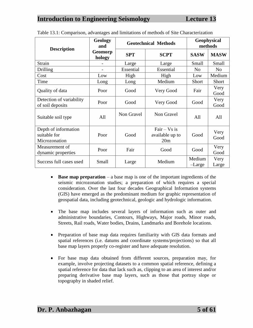
Table 13.1: Comparison, advantages and limitations of methods of Site Characterization
Base map preparation – a base map is one of the important ingredients of the
seismic microzonation studies; a preparation of which requires a special
consideration. Over the last four decades Geographical Information systems
(GIS) have emerged as the predominant medium for graphic representation of
geospatial data, including geotechnical, geologic and hydrologic information.
The base map includes several layers of information such as outer and
administrative boundaries, Contours, Highways, Major roads, Minor roads,
Streets, Rail roads, Water bodies, Drains, Landmarks and Borehole locations.
Preparation of base map data requires familiarity with GIS data formats and
spatial references (i.e. datums and coordinate systems/projections) so that all
base map layers properly co-register and have adequate resolution.
For base map data obtained from different sources, preparation may, for
example, involve projecting datasets to a common spatial reference, defining a
spatial reference for data that lack such as, clipping to an area of interest and/or
preparing derivative base map layers, such as those that portray slope or
topography in shaded relief.
Description
Geology
and
Geomorp
hology
Geotechnical Methods Geophysical
methods
SPT SCPT SASW MASW
Strain - Large Large Small Small
Drilling - Essential Essential No No
Cost Low High High Low Medium
Time Long Long Medium Short Short
Quality of data Poor Good Very Good Fair Very
Good
Detection of variability
of soil deposits Poor Good Very Good Good
Very
Good
Suitable soil type All Non Gravel
Non Gravel
All All
Depth of information
suitable for
Microzonation
Poor Good
Fair – Vs is
available up to
20m
Good Very
Good
Measurement of
dynamic properties Poor Fair Good Good
Very
Good
Success full cases used Small Large Medium Medium
–Large
Very
Large
Introduction to Engineering Seismology Lecture 13
Dr. P. Anbazhagan 6 of 61
Steps involved
1. Define region of interest for current project
2. Decide which datasets are valuable to your project
3. Identify sources of datasets and download to local computer
a. Topographic
b. Thematic
c. Imagery
4. Identify and georeference any additional non-digital sources of spatial
data
a. Compile tabular data with x,y location information into a
spreadsheet and add to GIS application
b. Scan paper map products
i. Clip scanned image to area of interest and save as
compatible file format (tiff, jpeg)
ii. Georeference scanned image
5. Confirm that all datasets are in the same coordinate system, projection
and datum.
a. If coordinate system is undefined, find original coordinate
system and establish spatial reference
b. If not all the same, project to a common coordinate system and
datum
6. Prepare topographic derivatives such as slope or hill shade layers
7. Clip all spatial data to a common project area extent
Available data collection - The major contributions for the microzonation
studies are the probabilistic assessment of the regional earthquake hazard,
interpretation of the microtremor records, and interpretation of the available
geological and geotechnical data based on a grid approach
The compilation of the available Geological and Geotechnical data and
additional subsurface explorations are carried out to supplement the available
data.
Evaluation and analysis of the available geotechnical data is done to determine
the necessary parameters for conducting the microzonation with respect to
different parameters.
For the identification of the local soil conditions, an approach was chosen by
taking available existing data into account.
Data are available from different sources, with varying degree of information
on the site investigations being conducted, reliability and quality of the derived
data.

Introduction to Engineering Seismology Lecture 13
Dr. P. Anbazhagan 7 of 61
Plausibility check of the available data is essential prior to carrying out the
microzonation procedure; direct use of this kind of data from such a variety of
different sources might lead to an unrealistic scenario, and might not be
comparable or even withstand a subsequent confirmation of this approach in
terms of the hypothetical boreholes.
Nonetheless data from different sources should be taken into account if the
quality appears to be acceptable so that it is possible to benefit from an
independent view of the soil conditions in overall terms and the reliability of a
single site investigation in particular.
Topic 2
3-D Subsurface Modeling of Geotechnical Data Using GIS
Geographical information system (GIS) based subsurface model is developed
which helps in data management, develop geostatistical functions, 3-
dimensional (3-D) visualization of subsurface with geo-processing capability
and future scope for web based subsurface mapping tool. The three major
outcomes are:
1. Development of digitized map of the area with layers of
information
2. Development of GIS database for collating and synthesizing
geotechnical data available with different sources
3. Development of 3-dimensional view of subsoil strata presenting
various geotechnical properties such as location details, physical
properties, grain size distribution, Atterberg limits, SPT ‗N‘ values
and strength properties for soil and rock along with depth in
appropriate format.
The 3-D subsurface model with geotechnical data has been generated with base
map. The boreholes are represented as 3-dimensional objects projecting below
the base map layer up to the available borehole depth, geotechnical properties
are represented as layers at 0.5m intervals with SPT ‗N‘ values (Fig 13.1).
Each borehole is attached with geotechnical data versus depth. Also scanned
image files of borelogs and properties table are attached to the location in plan.
The data consists of visual soil classification, standard penetration test results,
ground water level, time during which test has been carried out, and, other
physical and engineering properties of soil.
From this 3-D, geotechnical model, geotechnical information on any borehole
at any depth can be obtained at every 0.5m interval by clicking at that level
(donut).The model provides two options to view the data at each borehole

Introduction to Engineering Seismology Lecture 13
Dr. P. Anbazhagan 8 of 61
1. Visualize the soil character as colored layer with depth information
along with properties in excel format and
2. Bore logs and properties as an image file.
A
Fig 13 .1 : Typical Borehole in Three Dimensional View
Topic 3
Site characterization using Geological data
Earthquake damage is commonly controlled by three interacting factors-
source and path characteristics, local geological and geotechnical conditions
and type of the structures. Obviously, all of this would require analysis and
presentation of a large amount of geological, seismological and geotechnical
data.
The initial geological site characterization must focus on locating and
quantifying the most fractured zones, for it is these highly fractured areas that
will most significantly affect the evaluation of the site.
The response of a soil deposit is dependent upon the frequency of the base
motion and the geometry and material properties of the soil layer above the
bedrock. Seismic microzonation is the process of assessment of the source &
path characteristics and local geological & geotechnical characteristics to
provide a basis for estimating and mapping a potential damage to buildings, in
other words it is the quantification of hazard.
Seismic microzonation would start with the assessment of the local geological
formations and with the mapping of the surface geology based on available
information, site surveys, site investigations, and soil explorations. The
purpose is to determine the boundaries and the characteristics of the geological
formation and to prepare a geology map at a scale of 1:5000 or larger.

Introduction to Engineering Seismology Lecture 13
Dr. P. Anbazhagan 9 of 61
This map clearly indicates the geological formations and their variation
however, it is important, as pointed out by Willis et al., (2000), to base the site
classification on measured characteristics of geologic units taking into
consideration the possible variations in each unit. The deviations from the
mean values obtained for each geological unit may exceed the permissible
limits to justify its use for assessing the effects of local soil conditions.
Wills and Silva (1998) suggested using average shear wave velocity in the
upper 30 m as one parameter to characterize the geological units while also
admitting the importance of other factors such as impedance contrast, 3-
dimensional basin and topographical effects, and source effects such as rupture
directivity on ground motion characteristics.
Topic 4
Variation of rock depth or soil overburden thickness
Spatial variability of the bed/hard rock with reference to ground surface is vital
for many applications in geosciences. Rock depth in a site is very useful
parameter to the geotechnical earthquake engineers to find their basic
requirement of hard strata and ground motion at rock level.
In the ground response analysis, Peak Ground Acceleration (PGA) and
response spectrum for the particular site is evaluated at the rock depth levels
and further on at the ground level considering local site effects. This is an
essential step to evaluate site amplification and liquefaction hazards of a site
and further to estimate induced forces on the structures.
In ground response analysis, the response of the soil deposit is determined
from the motion at the bed rock level. In all these problems, it is essential to
evaluate the depth of the hard rock from the ground level.
With an objective of predicting the spatial variability of the reduced level of
the bed/hard rock in Bangalore, an attempt has been made to develop models
based on Ordinary Kriging technique, Artificial Neural Network (ANN) and
Support Vector Machine (SVM). It is also aimed at comparing the
performance of these developed models for the available data in Bangalore.
The kriging method was developed during the 1960s and 1970s and has been
acknowledged as a good spatial interpolator (Matheron 1963; Isaaks and
Srivastava 1989; Davis 2002). The most important features of this method are
1. The unbiased estimate of results,
2. The minimum estimation error, and
3. Uncertainty evaluation of interpolation data points.

Introduction to Engineering Seismology Lecture 13
Dr. P. Anbazhagan 10 of 61
The main goal of kriging is to predict the unknown properties from the
knowledge of semi-variogram. Semi-variogram is the analytical tool used to
evaluate and quantify the degree of spatial autocorrelation. The semi-
variogram is an appreciation of the dispersion of the parameters, which equates
to the variance and also gives an autocorrelation distance that represents the
radius of influence of a measurement made at a given point.
Further, it provides the type of variability that indicates how values fluctuate in
space. A new method for cross-validation analysis of developed models has
been also proposed and validated. The cross-validation of the model has been
done based on the examination of residuals.
Topic 5
Geotechnical Explorations for Site Characterization
Scope of the investigation always depends upon the purpose of the study.
Investigations for the seismic microzonation are similar in many respects to
regular investigations. The main difference is the scale of the study. In general
geotechnical Investigations are of smaller size covering few meters to
hundreds of acres depending upon the size of the building or any other
proposed construction. In case of seismic microzonation, the extent of the
investigations to be covered varies from few square kilometers to hundreds of
square kilometers.
Geotechnical engineering analysis and evaluation is valid only if the measured
values are representative of in situ conditions. Properties of some materials are
best measured in the laboratory, while others in field tests. The general
objective of the geotechnical/geophysical investigation for the microzonation
is to account for all the significant factors that influence the seismic hazards.
This objective is achieved only through proper planning of in situ and
laboratory testing.
Geotechnical investigation involves the following tasks for the purpose of
microzonation.
1. Need to define/identify the bedrock depth, which is very important
as purpose of the geotechnical investigations is to assess the
influence of local site conditions on the bedrock/earthquake motions.
2. Obtain surface mapping to account influence of topography features
and geomorphology conditions on the expected levels of earthquake
shaking. Arrive at the topography and identify geological hazards if
any, such as unstable slopes, faults, floodplains
3. Define groundwater table conditions considering seasonal variations
4. Perform in situ testing and procure samples for laboratory testing
Introduction to Engineering Seismology Lecture 13
Dr. P. Anbazhagan 11 of 61
Various geotechnical tests including both in situ and laboratory tests are
available for seismic microzonation which are discussed at length in the
coming section. However, it is important to mention that such geotechnical
investigations are suitable for depths upto 50 to 60 m, beyond these depths,
undisturbed sampling becomes difficult.
Topic 6
Standard Penetration Test (SPT)
The standard penetration test is done using a split- spoon sampler in a
borehole / auger hole. This sampler consists of a driving shoe, a split- barrel of
circular cross-section (longitudinally split into two parts) and a coupling. The
procedure for carrying out the standard penetration test is discussed as follows
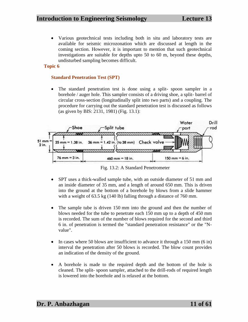
(as given by BIS: 2131, 1981) (Fig. 13.1):
Fig. 13.2: A Standard Penetrometer
SPT uses a thick-walled sample tube, with an outside diameter of 51 mm and
an inside diameter of 35 mm, and a length of around 650 mm. This is driven
into the ground at the bottom of a borehole by blows from a slide hammer
with a weight of 63.5 kg (140 lb) falling through a distance of 760 mm.
The sample tube is driven 150 mm into the ground and then the number of
blows needed for the tube to penetrate each 150 mm up to a depth of 450 mm
is recorded. The sum of the number of blows required for the second and third
6 in. of penetration is termed the "standard penetration resistance" or the "N-
value".
In cases where 50 blows are insufficient to advance it through a 150 mm (6 in)
interval the penetration after 50 blows is recorded. The blow count provides
an indication of the density of the ground.
A borehole is made to the required depth and the bottom of the hole is
cleaned. The split- spoon sampler, attached to the drill-rods of required length
is lowered into the borehole and is relaxed at the bottom.
Introduction to Engineering Seismology Lecture 13
Dr. P. Anbazhagan 12 of 61
The sampler is then driven to a distance of 450 mm in three intervals of 150
mm each. This is done by dropping a hammer of 63.5 kg from a height of 762
mm (BIS: 2131, 1981). The number of blows required to penetrate the soil is
noted down for the last 300 mm, and this is recorded as the N value. The
number of blows required to penetrate the sampler through the first 150 mm is
called the seating drive and is disregarded. This is because the soil for the first
150 mm is disturbed and is ineffective for the SPT- N value.
The sampler is then pulled out and is detached from the drill rods. The soil
sample, within the split barrel, is collected taking all precautions so as to not
disturb the moisture content and is then transported to the laboratory, for tests.
Sometimes, a thin liner is placed inside the split barrel. This makes it feasible
for collecting the soil sample, within the liner, by sealing off both the ends of
the liner with molten wax and then taking it away for laboratory test of the
contained soil.
The standard penetration test is performed at every 0.75 m intervals in a
borehole. If the depth of the borehole is large, however, the interval can be
made 1.50 m. In case, the soil under consideration consists of rocks or
boulders, the SPT- N value can be recorded for the first 300 mm. The test is
stopped if:
1. 50 blows are required for any 150 mm penetration
2. 100 blows are required for any 300 mm penetration
3. 10 consecutive blows produce no advance
However, it should be noted that the SPT- N value obtained from the above
set of procedures has to be corrected before it can be used for any of the
empirical relations. These corrections and their values for certain conditions
have been discussed in detail in the next section.
Topic 7
Corrections Applied for SPT “N” Values
The SPT data collected is field ‗N‘ values with out applying any corrections.
Usually for engineering use of site response studies and liquefaction analysis
the SPT ―N‖ values has to be corrected with various corrections and a seismic
borelog has to be obtained.
The seismic bore log contains information about depth, observed SPT ‗N‘
values, density of soil, total stress, effective stress, fines content, correction
factors for observed ―N‖ values, and corrected ―N‖ value.
The ‗N‘ values measured in the field using Standard penetration test procedure
have been corrected for various corrections, such as:
Introduction to Engineering Seismology Lecture 13
Dr. P. Anbazhagan 13 of 61
1. Overburden Pressure (CN),
2. Hammer energy (CE),
3. Borehole diameter (CB),
4. presence or absence of liner (CS),
5. Rod length (CR) and
6. fines content (Cfines)
Corrected ‗N‘ value i.e., 601)(N is obtained using the following equation:
1 60( ) ( N E B S RN N C C C C C
Correction for Overburden Pressure - The effective use of SPT blow count
for seismic study requires the effects of soil density and effective confining
stress on penetration resistance to be separated. Consequently, Seed et al
(1975) included the normalization of penetration resistance in sand to an
equivalent w of one atmosphere as part of the semi empirical procedure.
SPT N-values recorded in the field increases with increasing effective
overburden stress; hence overburden stress correction factor is applied (Seed
and Idriss 1982). This factor is commonly calculated from equation developed
by Liao and Whitman (1986).
However Kayen et al. (1992) suggested the following equation, which limits
the maximum CN value to 1.7 and provides a better fit to the original curve
specified by Seed and Idriss (1982):
Where, w = effective overburden pressure, Pa = 100 kPa, and CN should not
exceed a value of 1.7. This empirical overburden correction factor is also
recommended by Youd et al (2001). For high pressures (300kPa), which are
generally below the depth for which the simplified procedure has been
verified, CN should be estimated by other means (Youd et al, 2001).
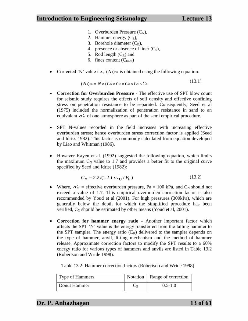
Correction for hammer energy ratio - Another important factor which
affects the SPT ‗N‘ value is the energy transferred from the falling hammer to
the SPT sampler. The energy ratio (ER) delivered to the sampler depends on
the type of hammer, anvil, lifting mechanism and the method of hammer
release. Approximate correction factors to modify the SPT results to a 60%
energy ratio for various types of hammers and anvils are listed in Table 13.2
(Robertson and Wride 1998).
Table 13.2: Hammer correction factors (Robertson and Wride 1998)
Type of Hammers Notation Range of correction
Donut Hammer CE 0.5-1.0
)/'2.1/(2.2 aPoCN
(13.1)
(13.2)

Introduction to Engineering Seismology Lecture 13
Dr. P. Anbazhagan 14 of 61
Because of variations in drilling and testing equipment and differences in
testing procedures, a rather wide range in the energy correction factor CER has
been observed as noted in the table. Even when procedures are carefully
monitored to confirm the established standards some variation in CE may occur
because of minor variations in testing procedures.
Measured energies at a single site indicate that variations in energy ratio
between blows or between tests in a single borehole typically vary by as much
as 10%. The workshop participants of NCEER 1996 & 1998 (Youd et al,
2001) recommend measurement of the hammer energy frequently at each site
where the SPT is used.
Where measurements cannot be made, careful observation and notation of the
equipment and procedures are required to estimate a CE value. Use of good-
quality testing equipment and carefully controlled testing procedures will
generally yield more consistent energy ratios.
For Liquefaction calculation Yilmaz and Bagci (2006) had taken the CE value
as 0.7 for SPT hammer energy donut type for soil liquefaction susceptibility
and hazard mapping in Kutahya, Turkey. Similar kind of hammer is used for
soil investigations; hence the value of 0.7 is taken for CE.
Other correction factors - The other correction factors adopted such as
correction for borehole diameter, rod length and sampling methods modified
from Skempton (1986) and listed by Robertson and Wride (1998) are
presented in Table 13.2.
Correction for borehole diameter (CB) is used as 1.05 for 150 mm borehole
diameter, Rod length (CR) is taken from the Table 13.3, based on the rod
length the presence or absence of liner (CS) is taken as 1.0 for standard
sampler.
The corrected ―N‖ Value (N1)60 is further corrected for fines content based on
the revised boundary curves derived by Idriss and Boulanger (2004) for
cohesionless soils as described below:
Safety Hammer CE 0.7-1.2
Automatic-trip Donut Hammer CE 0.8-1.3
601601601 )()()( NNN cs
2
601001.0
7.15
001.0
7.963.1exp)(
FCFCN
(13.3)
(13.4)
Introduction to Engineering Seismology Lecture 13
Dr. P. Anbazhagan 15 of 61
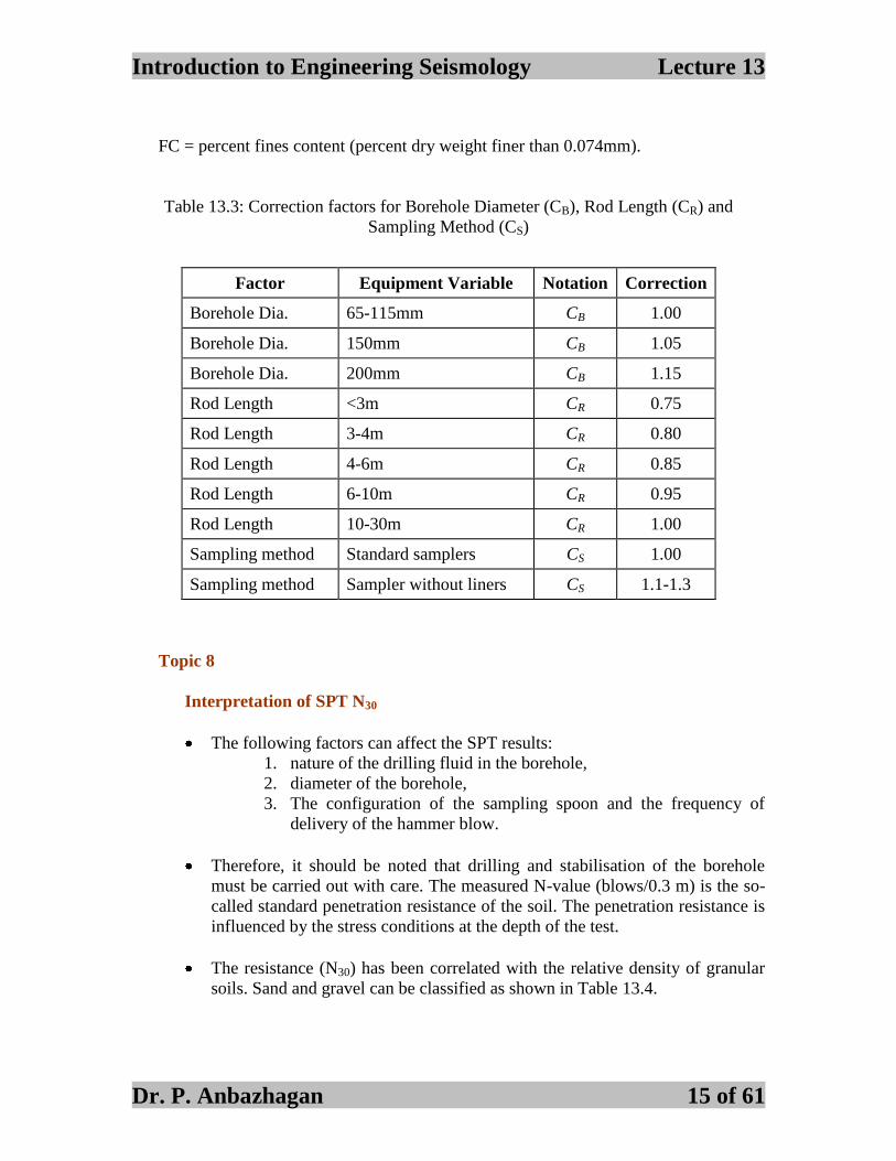
FC = percent fines content (percent dry weight finer than 0.074mm).
Table 13.3: Correction factors for Borehole Diameter (CB), Rod Length (CR) and
Sampling Method (CS)
Factor Equipment Variable Notation Correction
Borehole Dia. 65-115mm CB 1.00
Borehole Dia. 150mm CB 1.05
Borehole Dia. 200mm CB 1.15
Rod Length <3m CR 0.75
Rod Length 3-4m CR 0.80
Rod Length 4-6m CR 0.85
Rod Length 6-10m CR 0.95
Rod Length 10-30m CR 1.00
Sampling method Standard samplers CS 1.00
Sampling method Sampler without liners CS 1.1-1.3
Topic 8
Interpretation of SPT N30
The following factors can affect the SPT results:
1. nature of the drilling fluid in the borehole,
2. diameter of the borehole,
3. The configuration of the sampling spoon and the frequency of
delivery of the hammer blow.
Therefore, it should be noted that drilling and stabilisation of the borehole
must be carried out with care. The measured N-value (blows/0.3 m) is the so-
called standard penetration resistance of the soil. The penetration resistance is
influenced by the stress conditions at the depth of the test.
The resistance (N30) has been correlated with the relative density of granular
soils. Sand and gravel can be classified as shown in Table 13.4.

Introduction to Engineering Seismology Lecture 13
Dr. P. Anbazhagan 16 of 61
Ta b le 13 .4 : Classification of sand and gravel
The sources of some of the common errors while carrying out SPT tests are
listed in Table 13.5 (Kulhawy and Mayne, 1990).
Table 13.5: Source of errors in SPT test
Cause Effects Influence on
SPT-N value
Inadequate cleaning of hole SPT is not made in original in-situ soil.
Therefore, spoils may become trapped in
sampler and be compressed as sampler is
driven, reducing recovery
Increases
Failure to maintain adequate
head of water in borehole
Bottom of borehole may become quick
and soil may rinse into the hole
Decreases
Careless measure of hammer
drop
Hammer energy varies
Increases
Hammer weight inaccurate Hammer energy varies Increases or
Decreases
Hammer strikes drill rod
collar eccentrically
Hammer energy reduced Increases
Lack of hammer free fall
because of ungreased
sheaves, new stiff rope on
weight, more than two turns
on cathead, incomplete
release of rope each drop
Hammer energy reduced Increases
Sampler driven above
bottom of casing
Sampler driven in disturbed,
artificially densified soil
Increases
greatly
Careless blow count Inaccurate results Increases or
Decreases
Use of non-standard sampler Corrections with standard
sampler not valid
Increases or
Decreases
Coarse gravel or cobbles in
soil
Sampler becomes clogged or
impeded
Increases
Use of bent drill rods Inhibited transfer of energy of sampler Increases
SPT N Value Relative density Classification
0-4 0 -15 Very loos e
4 -10 15 -35 Loos e
10 -30 35 -65 Mediu m den s e
30 -50 65 -85 Den s e
>50 85 -100 Very den s e

Introduction to Engineering Seismology Lecture 13
Dr. P. Anbazhagan 17 of 61
Topic 9
Geotechnical Laboratory tests
Routine Geotechnical laboratory tests (following relevant IS codes wherever
applicable) for soils and rock samples are as follows:
Index properties of Soil and Rock Samples - For Soil samples: Grain Size
Analysis of the representative samples can be obtained from Sieve and
Hydrometer analysis, (BIS: 2720 Part 4-1985) or deploying laser analyzer
(BIS: 2720 Part 4-1985). This is to evaluate the soil particle sizes and
gradation. Coarser particles are separated in the sieve analysis portion, and the
finer particles are analyzed with a hydrometer (75 μm). Size is chosen to make
a distinction between coarse and fine particles). The sieve analysis is done
using an automatic sieve shaker where in the sample passes through
progressively to smaller mesh sizes to assess its gradation. The hydrometer
analysis uses the rate of sedimentation to determine particle gradation.
The Atterberg limits are a basic measure of the nature of a fine-grained soil.
Depending on the water content of the soil, it may appear in any of the four
states: solid, semi-solid, plastic and liquid. In each state the consistency and
behavior of a soil is different and thus so are its engineering properties. Thus,
the boundary between each state can be defined based on a change in the soil's
behavior and they are represented by Atterberg Limits (Liquid Limit, LL;
Plastic Limit, PL; Shrinkage Limit, SL). These Atterberg limits can be
determined in the laboratory following BIS: 2720(Part 5) -1985. The
difference between liquid limit and plastic limit is called the plasticity index
(IP). The shrinkage limit (SL) is the water content where further loss of
moisture will not result in any more volume reduction.
Natural water content (w %) can be calculated as per BIS: 2720 Part 2-1973.
Specific Gravity, In-situ Density and Moisture Content can be obtained as per
BIS: 2720 Part 3-1980. Relative Density of cohesionless soils can be
evaluated as described in BIS: 2720 Part 14-1983. Free swell index of soil as
per BIS: 2720 (Part XL) – 1977 also termed as free swell or differential free
swell is the increase in volume of soil without any external constraint when
subjected to submergence in water. Bulk density (γ) is defined as the mass of
soil particles of the material divided by the total volume they occupy.
Permeability characteristics of the soils can be determined using falling head
or fixed head Permeameter as per BIS: 2720 (Part17)-1986. Compressibility
characteristics can be obtained from Oedometer tests as per Bureau of Indian
Standards (BIS: 2720 (Part15)-1986). Strength characteristics can also be
obtained using triaxial, direct shear and vane shear tests.
Introduction to Engineering Seismology Lecture 13
Dr. P. Anbazhagan 18 of 61
For Rock Samples: Following tests along with BIS codes are used for rock
samples:
1. Unconfined Compressive Strength of rock samples [BIS:9143-
1979]
2. Dynamic Modulus of rock core specimen, [BIS:10782-1983]
3. Modulus of Elasticity, Poisson‘s Ratio, in uniaxial compression
[BIS:9221-1979]
4. Point Load Strength Index [BIS:8764-1998]
Tests for shear strength parameters and consolidation characteristics -
Tests for shear and consolidation shall be preferably performed on
undisturbed samples and in some cases on remoulded samples. The direct
shear test (Direct shear Test: BIS:2720 PART 13-1986) determines the
consolidated drained strength properties of a sample. Test is performed with
different normal loads to evaluate the shear strength parameters (c and φ).
Methods of test for soils for determination of Shear Strength parameters of
soil from consolidated undrained triaxial compression test with or without
pore water measurement are provided in BIS 2720 (Part XII) – 1981. Triaxial
Shear tests comprise UU, CU (Consolidated Undrained test with and without
Pore Water Pressure Measurement) or CD (consolidated drained) tests.
Topic 10
Site Classification using SPT data
GIS database for collating and synthesizing geotechnical data available with
different sources and 3-dimensional view of soil stratum presenting various
geotechnical parameters with depth in appropriate format should be developed.
In the context of prediction of reduced level of rock (called as ―engineering
rock depth‖ corresponding to about SPT ―N‖ >100) in the subsurface and their
spatial variability evaluated using Artificial Neural Network (ANN).
Observed SPT ‗N‘ values are corrected by applying necessary corrections,
which can be used for engineering studies such as site response and
liquefaction analysis.
The site characterization is attempted using geotechnical bore log data and
standard penetration test ―N‖ values. The Standard Penetration Test (SPT) is
one of the oldest, most popular, and commonly used in situ test for exploration
in soil mechanics and foundation engineering because the equipment and test
procedures are simple.
The Standard Penetration Test (SPT) is particularly useful for seismic site
characterizations, site response, and liquefaction studies towards seismic
Introduction to Engineering Seismology Lecture 13
Dr. P. Anbazhagan 19 of 61
microzonation. In most cases the site specific response analysis, shear wave
velocity, and shear modulus (Gmax) of layers are estimated using relationships
based on the SPT N values (Anbazhagan and Sitharam, 2010).
Topic 11
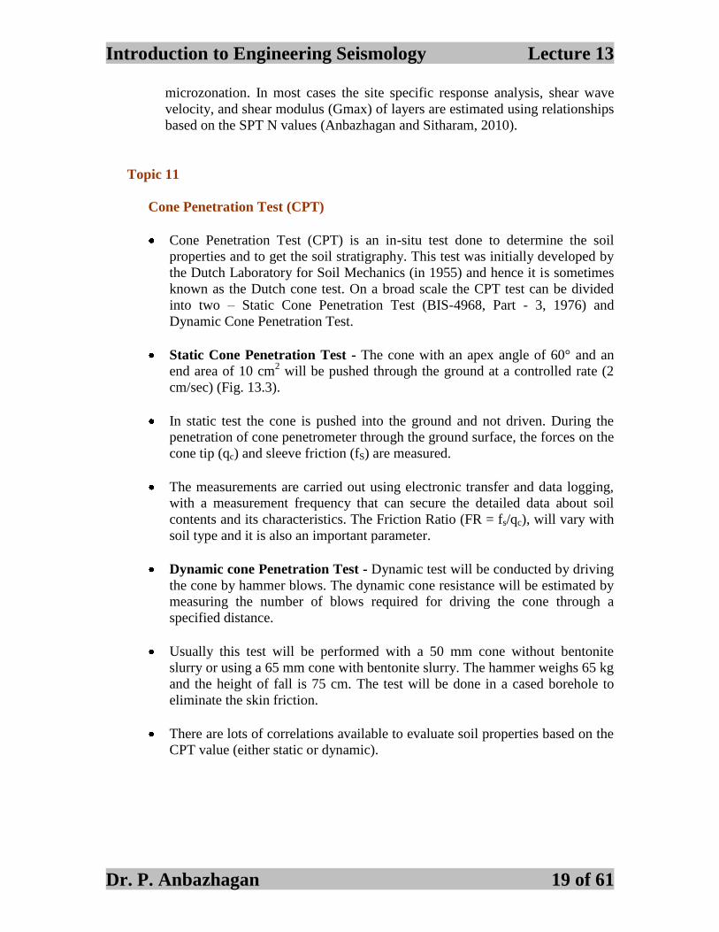
Cone Penetration Test (CPT)
Cone Penetration Test (CPT) is an in-situ test done to determine the soil
properties and to get the soil stratigraphy. This test was initially developed by
the Dutch Laboratory for Soil Mechanics (in 1955) and hence it is sometimes
known as the Dutch cone test. On a broad scale the CPT test can be divided
into two – Static Cone Penetration Test (BIS-4968, Part - 3, 1976) and
Dynamic Cone Penetration Test.
Static Cone Penetration Test - The cone with an apex angle of 60° and an
end area of 10 cm2 will be pushed through the ground at a controlled rate (2
cm/sec) (Fig. 13.3).
In static test the cone is pushed into the ground and not driven. During the
penetration of cone penetrometer through the ground surface, the forces on the
cone tip (qc) and sleeve friction (fS) are measured.
The measurements are carried out using electronic transfer and data logging,
with a measurement frequency that can secure the detailed data about soil
contents and its characteristics. The Friction Ratio (FR = fs/qc), will vary with
soil type and it is also an important parameter.
Dynamic cone Penetration Test - Dynamic test will be conducted by driving
the cone by hammer blows. The dynamic cone resistance will be estimated by
measuring the number of blows required for driving the cone through a
specified distance.
Usually this test will be performed with a 50 mm cone without bentonite
slurry or using a 65 mm cone with bentonite slurry. The hammer weighs 65 kg
and the height of fall is 75 cm. The test will be done in a cased borehole to
eliminate the skin friction.
There are lots of correlations available to evaluate soil properties based on the
CPT value (either static or dynamic).
Introduction to Engineering Seismology Lecture 13
Dr. P. Anbazhagan 20 of 61
Fig. 13.3: Different types of Cones used in CPT test
(http://geosystems.ce.gatech.edu/Faculty/Mayne/Research/devices/cpt.htm)
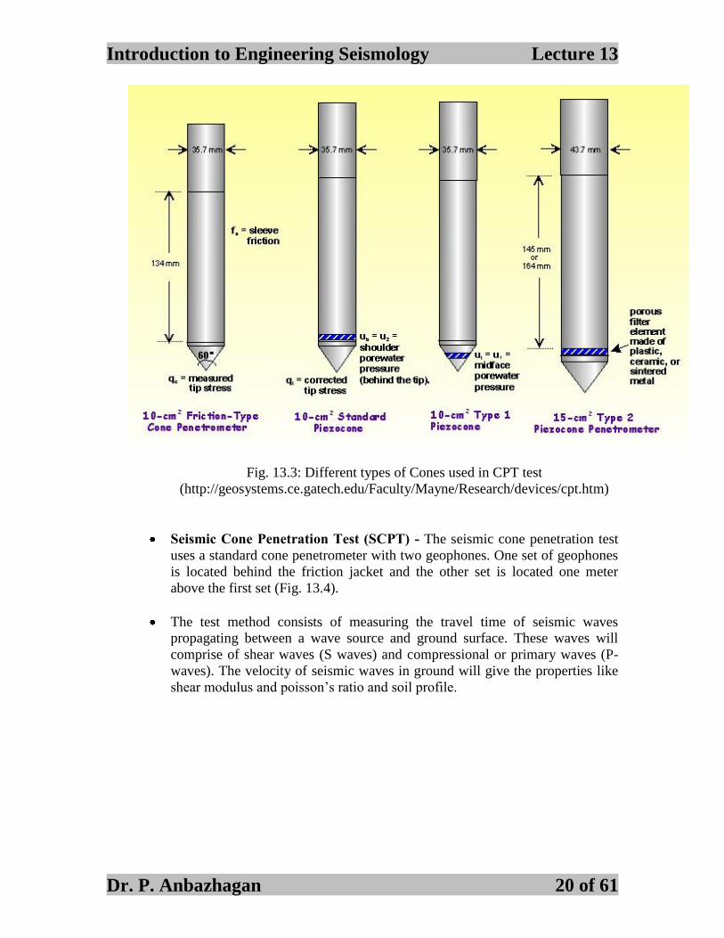
Seismic Cone Penetration Test (SCPT) - The seismic cone penetration test
uses a standard cone penetrometer with two geophones. One set of geophones
is located behind the friction jacket and the other set is located one meter
above the first set (Fig. 13.4).
The test method consists of measuring the travel time of seismic waves
propagating between a wave source and ground surface. These waves will
comprise of shear waves (S waves) and compressional or primary waves (P-
waves). The velocity of seismic waves in ground will give the properties like
shear modulus and poisson‘s ratio and soil profile.
Introduction to Engineering Seismology Lecture 13
Dr. P. Anbazhagan 21 of 61
Fig. 13.4: Seismic Cone Penetration test (Fugro Company)
Topic 12
Site Characterization by Cone Penetration Testing
Cone penetration testing (CPT) is a fast and reliable means of conducting site
investigations for exploring soils and soft ground for support of embankments,
retaining walls, pavement subgrade, bridge foundations etc. The CPT
soundings can be used either as a replacement or complement to conventional
rotary drilling and sampling methods.

Introduction to Engineering Seismology Lecture 13
Dr. P. Anbazhagan 22 of 61
In CPT, an electronic steel probe is hydraulically pushed to collect continuous
readings of point load, friction, and pore water pressures with typical depths up
to 30 m (100 ft) or more reached in about 1 to 11⁄2 h.
Data are logged directly to a field computer and can be used to evaluate the
geostratigraphy, soil types, water table, and engineering parameters of the
ground by the geotechnical engineer on-site, thereby offering quick and
preliminary conclusions for design. With proper calibration, using full-scale
load testing coupled with soil borings and lab- oratory testing, the CPT results
can be used for final design parameters and analysis.
In its simplest application, the cone penetrometer offers a quick, expedient, and
economical way to profile the subsurface soil layering at a particular site. No
drilling, soil samples, or spoils are generated; therefore, CPT is less disruptive
from an environmental standpoint.
The continuous nature of CPT readings permit clear delineations of various
soil strata, their depths, thicknesses, and extent, perhaps better than
conventional rotary drilling operations that use a standard drive sampler at 5-ft
vertical intervals. Therefore, if it is expected that the subsurface conditions
contain critical layers or soft zones that need detection and identification, CPT
can locate and highlight these particular features.
Topic 13
Corrections to CPT
For electric cones that record pore pressure, corrections can be made to
account for unequal end area effects. Baligh et al. (1981) and Campanella et al
(1982) proposed that the cone resistance, qc, could be corrected to a total cone
resistance, qt, using the following expression:
where u is pore pressure measured between the cone tip and the friction sleeve
and a is net area ratio. It is often assumed that the net area ratio is given by
where d is diameter of load cell support and D is diameter of cone. However,
this provides only an approximation of the net area ratio, since additional
friction forces are developed due to distortion of the water seal O-ring.
Therefore, it is recommended that the net area ratio should always be
determined ‗in a small caliion vessel (Battaglio and Mankcalco 1983;
Campanella and Robertson 1988). A similar correction can also be applied to
2
2
D
da
uaqq ct )1( (13.5)
(13.6)
Introduction to Engineering Seismology Lecture 13
Dr. P. Anbazhagan 23 of 61
the sleeve friction (Iunne ez al. 1986; Konrad 1987). Konrad (1981) suggested
the following expression for the total stress sleeve friction, ft:
Where, sb
st
A
Ab ,
s
sb
A
Ac ,
u
us
Ast is end area of friction sleeve at top, Asb is end area of friction sleeve at
bottom, As, is outside surfacea area of friction sleeve, and us, is pore pressure
at top of friction sleeve.
However, to apply this correction, pore pressure data are required at both ends
of the friction sleeve. Konrad (1987) showed that this correction could be more
than 30% of the measured fs, for some cones. However, the correction can be
significantly reduced for cones with an equal end area friction sleeve (i.e.,
b=1.0).
The corrections in cone resistance and sleeve friction are only important in soft
clays and silts where high pore pressure and low cone resistance occur. The
corrections are negligible in cohensionless soils where penetration is generally
drained and cone resistance is generally large. The author believes that the
correction to the sleeve friction is generally unnecessary provided the cone has
an equal end area friction sleeve.
Topic 14
CPT Profile, Downhole Memphis
By recording three continuous measurements vertically with depth, the CPT is
an excellent tool for profiling strata changes, delineating the interfaces between
soil layers, and detecting small lenses, inclusions, and stringers within the
ground.
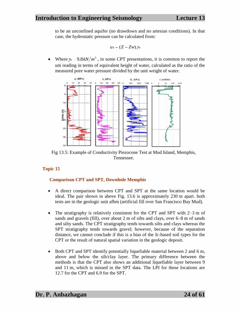
The data presentation from a CPT sounding should include the tip, sleeve, and
porewater readings plotted with depth in side-by-side graphs, as shown in
Figure 13.5.
The total cone tip resistance (qt) is always preferred over the raw measured
value (qc). For SI units, the depth (z) is presented in meters (m), cone tip
stress(qt) in either Pascal (MPa or kPa), and sleeve resistance (fs) and
porewater pressure (um) in kPa.
If the depth of the water table is known (Zw), it is convenient to show the
hydrostatic pore water pressure (u0), if the groundwater regime is understood
cubff st )1((13.7)
(13.8)
Introduction to Engineering Seismology Lecture 13
Dr. P. Anbazhagan 24 of 61
to be an unconfined aquifer (no drawdown and no artesian conditions). In that
case, the hydrostatic pressure can be calculated from:
Where 38.9 mkNw , in some CPT presentations, it is common to report the
um reading in terms of equivalent height of water, calculated as the ratio of the
measured pore water pressure divided by the unit weight of water.
Fig 13.5: Example of Conductivity Piezocone Test at Mud Island, Memphis,
Tennessee.
Topic 15
Comparison CPT and SPT, Downhole Memphis
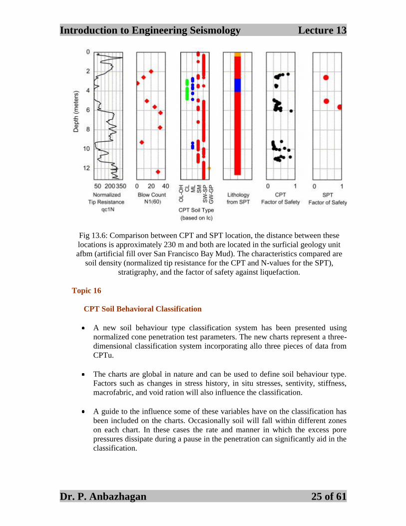
A direct comparison between CPT and SPT at the same location would be
ideal. The pair shown in above Fig. 13.6 is approximately 230 m apart. both
tests are in the geologic unit afbm (artificial fill over San Francisco Bay Mud).
The stratigraphy is relatively consistent for the CPT and SPT with 2–3 m of
sands and gravels (fill), over about 2 m of silts and clays, over 6–8 m of sands
and silty sands. The CPT stratigraphy tends towards silts and clays whereas the
SPT stratigraphy tends towards gravel; however, because of the separation
distance, we cannot conclude if this is a bias of the Ic-based soil types for the
CPT or the result of natural spatial variation in the geologic deposit.
Both CPT and SPT identify potentially liquefiable material between 2 and 6 m,
above and below the silt/clay layer. The primary difference between the
methods is that the CPT also shows an additional liquefiable layer between 9
and 11 m, which is missed in the SPT data. The LPI for these locations are
12.7 for the CPT and 6.9 for the SPT.
wZwZu ).(0
Introduction to Engineering Seismology Lecture 13
Dr. P. Anbazhagan 25 of 61
Fig 13.6: Comparison between CPT and SPT location, the distance between these
locations is approximately 230 m and both are located in the surficial geology unit
afbm (artificial fill over San Francisco Bay Mud). The characteristics compared are
soil density (normalized tip resistance for the CPT and N-values for the SPT),
stratigraphy, and the factor of safety against liquefaction.
Topic 16
CPT Soil Behavioral Classification
A new soil behaviour type classification system has been presented using
normalized cone penetration test parameters. The new charts represent a three-
dimensional classification system incorporating allo three pieces of data from
CPTu.
The charts are global in nature and can be used to define soil behaviour type.
Factors such as changes in stress history, in situ stresses, sentivity, stiffness,
macrofabric, and void ration will also influence the classification.
A guide to the influence some of these variables have on the classification has
been included on the charts. Occasionally soil will fall within different zones
on each chart. In these cases the rate and manner in which the excess pore
pressures dissipate during a pause in the penetration can significantly aid in the
classification.

Introduction to Engineering Seismology Lecture 13
Dr. P. Anbazhagan 26 of 61
Some of the most comprehensive recent work on soil classification using
electric cone penetrometer data was presented by Douglas and Olsen (1981).
One important distinction made by them was that CPT classification charts
cannot be expected to provide accurate predictions of soil type based on grain
size distribution but can provide a guide to soil behaviour type.
The CPT data provide a repeatable index of the aggregate behavior of the in-
situ soil in the immediate area of the probe. An example of a soil classification
chart for electric CPT data is shown in Fig. 13.7 and details are given in Table
13.6
Fig 13.7: Simplified soil behavior type classification for standard electric friction
cone (Robertson et al. 1986)
Table 13.6: Soil Behavior Type from CPT Classification Index, Ic (after Jefferies and
Davies, 1993)
Soil Classification Zone Number* Range of CPT Index Ic Values
Organic Clay soils 2 Ic>3.22
Clays 3 2.82< Ic>3.22
Silt Mixtures 4 2.54< Ic>2.82
Sand Mixtures 5 1.90< Ic>2.54
Sands 6 1.25< Ic>1.90
Gravelly Sands 7 Ic<1.25
*Notes: Zone number as per Robertson SBT (1990)
Introduction to Engineering Seismology Lecture 13
Dr. P. Anbazhagan 27 of 61
Topic 17
CPT Tests to Evaluate Seismic Ground Hazards
A series of cone penetration tests (CPTs) are conducted for quantifying seismic
hazards, obtaining geotechnical soil properties, and conducting studies at
liquefaction sites. The seismic piezocone provides four independent
measurements for delineating the stratigraphy, liquefaction potential, and site
amplification parameters.
At the same location, two independent assessments of soil liquefaction
susceptibility can be made using both the normalized tip resistance (qc1N) and
shear wave velocity (Vs1). In lieu of traditional deterministic approaches, the
CPT data can be processed using probability curves to assess the level and
likelihood of future liquefaction occurrence.
The cone penetrometer system used in these tests included an anchored truck-
mounted hydraulic rig with field computer data acquisition and three
geophysics-type penetrometers (5-, 10-, and 15-ton capacity). Each
penetrometer consists of a 60° angled apex at the tip instrumented to measure
five independent readings: tip resistance (qc), sleeve friction (fs), vertical
inclination (i), penetration porewater pressure (either midface u1 or shoulder
u2), and downhole shear wave velocity (Vs). Shear waves are recorded at 1-m
depth intervals, whereas the other readings are obtained at a constant logging
rate, generally set between 1 and 5 cm/s.
The tip resistance (qc) is a point stress related to the soil strength and the
reading must be corrected for porewater pressure effects on unequal areas,
especially in clays and silts. The corrected value is termed qT. The sleeve
resistance relates to the interface friction between the penetrometer and soil.
Magnitudes of porewater pressure depend upon the permeability of the
medium and the shoulder filter element (or u2 position) is required for the tip
correction.
The tip resistance (qT), sleeve friction (fs) and pore pressure (u2) are used
together to characterize the subsurface layering, soil behavioral type, and
strength properties. Particularly important in seismic investigations, a cyclic
stress-based analysis of liquefaction-prone sediments is available using the qT
data.
The seismic piezocone test (SCPTu) includes both penetration readings and
down hole geophysical measurements in the same sounding, thus optimizing
data collection at a given location.
In the test procedure, the shear waves are generated by striking a horizontal
steel plank that is coupled to the ground under an outrigger. The downhole

Introduction to Engineering Seismology Lecture 13
Dr. P. Anbazhagan 28 of 61
geophone is oriented parallel to the plank to detect vertically propagating,
horizontally polarized shear waves. From the measured wave train at each
depth, a pseudo-interval shear wave velocity (Vs) is determined as the
difference in travel distance between any two successive events divided by the
difference in travel times.
The travel times are determined in two ways: (1) by visually inspecting the
recorded wave traces and subjectively identifying the first arrival, and (2) by a
rigorous post-processing technique known as cross-correlation to determine the
time shift between the entire wave trains from successive paired records.
Topic 18
Geophysical Explorations
General Geotechnical investigations involve the drilling of holes in the
ground, sampling at discrete points, and in situ or laboratory testing. This
methodology suits for exploration of smaller volume of soil and rock.
However, for seismic microzonation, one needs to carry explorations on larger
volumes. Geophysical methods overcome this drawback and some of the other
problems inherent in conventional geotechnical investigation techniques.
There are many geophysical methods available today. Most of the methods
can provide the profiles of continuous sections. Some of the techniques can
also provide stiffness properties of the ground, which are useful for seismic
microzonation. Geophysical techniques also help in locating cavities,
backfilled mine shafts and subsurface geological features such as faults and
discontinuities.
In seismic microzonation, it is required to obtain detailed subsurface profile
over the region of interest. It is difficult to carry conventional geotechnical
site explorations over such a large region. In addition, carrying geotechnical
site explorations over a large area is very expensive. Geophysical methods are
only alternative to avoid these difficulties. These methods provide lateral
variability of the near-surface materials beneath a site.
The general objective of the geophysical/geotechnical investigation for the
microzonation is to account all the significant factors that influence on the
seismic hazards. This objective is achieved only through the proper planning
of in situ and laboratory testing. Geotechnical engineering analysis and
evaluation is valid only when they are based on truly representative values of
natural materials. It is very difficult to obtain undisturbed samples particularly
in case of sandy soils. These problems are eliminated in the geophysical
methods. These methods are generally, carried on the ground at in situ
Introduction to Engineering Seismology Lecture 13
Dr. P. Anbazhagan 29 of 61
conditions. Geophysical methods carried for the purpose of seismic
microzonation, should aimed at the following information
o Depth of the bedrock
o Very small strain stiffness of the ground
o To study variability of soils
These methods can be used in the subsurface explorations even up to the
depths of 100 to 150 m below ground level. Beyond these depths especially in
alluvial belts, there are no techniques for evaluating the subsurface.
Topic 19
Surface Wave Methods
Many geophysical methods are attempted for seismic site characterization, but
widely used methods are Spectral Analysis of Surface Waves (SASW) and
Multichannel Analysis of Surface Waves (MASW). SASW and MASW are
surface wave methods widely used for many civil and earth science
applications
Historically, most of the surface wave applications have followed three
fundamental steps:
1. Acquisition
2. Dispersion Analysis
3. Seeking the layered-earth model (Vs, Vp, h, r, etc.)
The main topics of development in recent history have been field procedures
(data acquisition) and data processing (dispersion and inversion analyses).
Early pioneering work in surface waves goes back to 1950s when the steady
state method was first used by Van der Pol (1951) and Jones (1955).
At this time, it was based on the fundamental-mode (M0)-only Rayleigh wave
assumption and all other types of waves higher modes, body waves, etc. were
ignored. This method then evolved later to be more-commonly called
Continuous Surface Wave (CSW) method (Matthews et al., 1996).
In the meantime, the soil site inversion theory was refined by Tokimatsu et al.
(1991). Since the very early stage of the surface wave application, pavement
was found to be more complex than soil (Sezawa, 1938; Press and Dobrin,
1956), with a special type of guided wave called leaky waves that required a
complex-domain approach in solving wave equations (Jones, 1962; Vidale,
1964).
A modern computer approach was introduced later by Martincek (1994), but it
still produced limited results. 20th century when Jones (1961) and other
investigators used small vibrators as wave experienced a boom in the mid-

Introduction to Engineering Seismology Lecture 13
Dr. P. Anbazhagan 30 of 61
1980s when digital computers became popular. A brief coverage of this
historical development can be found in the 2005 special issue of JEEG (Journal
of Environmental and Engineering Geophysics) on the surface wave method.
Another historical overview can be found in Park and Ryden (2007).
Topic 20
Two-Receiver Approach (The SASW Method)
In early 80s, a two-receiver approach was introduced by investigators at the
University of Texas (UT), Austin, that was based on the Fast Fourier
Transform (FFT) analysis of phase spectra of surface waves generated by
using an impulsive source like the sledge hammer (Figure 13.8). It then
became widely used among geotechnical engineers and researchers. This
method was called Spectral Analysis of Surface Waves (SASW) (Heisey et
al., 1982).
The fundamental-mode (M0)-only Rayleigh wave assumption was used during
the early stages. Simultaneous multi-frequency (not mono-frequency)
generation from the impact seismic source and then separation by FFT during
the subsequent data processing stage greatly improved overall efficiency of
the method in comparison to earlier methods such as the continuous surface
wave (CSW) method. Since then, significant research has been conducted at
UT-Austin (Nazarian et al., 1983; Rix et al., 1991; Al-Hunaidi, 1992;
Gucunski and Woods, 1992; Aouad, 1993; Stokoe et al., 1994; Fonquinos,
1995; Ganji et al., 1998) and a more complete list of the publications on
SASW up to early 1990s can be found in ―Annotated bibliography on SASW‖
by Hiltunen and Gucunski (1994). The overall procedure of SASW is as
follows.
Figure 13.8: Schematic representation of overall procedure of the SASW method

Introduction to Engineering Seismology Lecture 13
Dr. P. Anbazhagan 31 of 61
a. Field setup with different separations (D‘s),
b. Data processing for phase velocity (Vph): Vph=2*pi*f / dp
(dp=phase difference, f=frequency, pi=3.14159265)), and
c. Wavelength (L) filtering criteria—compact dispersion curve
Earlier research of SASW method was focused on ways to enhance accuracy
of the fundamental-mode (M0) Rayleigh-wave dispersion curve through field
procedure and data processing efforts. Then soon came the speculation about
the possibility of the curve ―being more than M0‖ and subsequently higher
modes (HM‘s) were included in the studies (Roesset et al., 1990; Rix et al.,
1991; Tokimatsu et al., 1992; Stokoe et al., 1994). In consequence, the
concept of ―apparent (or effective)‖ dispersion-curve (Gucunski and Woods,
1992; Williams and Gucunski, 1995) was introduced that accounts for the
possible mixture of multiple influences rather than M0 alone (Fig. 13.9).
Once multiple modes were recognized and included, the field approach and
data processing techniques attempted to account for the multiple-mode
possibilities. Pavement investigation by SASW was regarded quite
challenging, especially for base layers, and the possibility of multi-modal
superimposition was speculated as being responsible for this. Reported
difficulties with SASW fit into the following three main categories:
Figure 13.9: The apparent dispersion concept in the SASW method.
1. Higher modes (HM‘s) inclusion that was previously
underestimated,
2. Inclusion of other types of waves (body, reflected and scattered
surface waves, etc.) (Sheu et al., 1988; Hiltunen and Woods, 1990;
Introduction to Engineering Seismology Lecture 13
Dr. P. Anbazhagan 32 of 61
Foti, 2000) that was also underestimated or not considered at all,
and
3. Data processing, for example, phase unwrapping (Al-Hunaidi,
1992) during the phase-spectrum analysis to construct a dispersion
curve.
Topic 21
Multichannel Approach (MASW)
In early 2000s, the MASW (Multichannel Analysis of Surface Waves) method
came into popular use among the geotechnical engineers. The term ―MASW‖
originated from the publication made on Geophysics by Park et al. (1999).
The project actually started in mid-90s at the Kansas Geological Survey
(KGS) by geophysicists who had been utilizing the seismic reflection
method—long used in the oil industry to image the interior of the earth for
depths of several kilometers. Called the high-resolution reflection method, it
was used to image very shallow depths of engineering interest (e.g., 100 m or
less).
It was in the mid-90s when KGS started a project to utilize surface waves.
Knowing the advantages with the multichannel method proven throughout
almost half-century of its history for exploration of natural resources, their
goal was a multichannel method to utilize surface waves mainly for the
purpose of geotechnical engineering projects.
From the extensive studies performed by SASW investigators, they
acknowledged that surface wave properties must be more complex than
previously assumed or speculated, and that the two-receiver approach had
clearly reached its limitation to handle the complexity.
Based on the normal notion that the number of channels used in seismic
exploration can directly determine resolving power of the method, they
utilized diverse techniques already available after a long history of seismic
data analysis (Telford et al., 1976; Robinson and Treitel, 1980; Yilmaz, 1987)
and also developed new strategies in field and data processing to detail surface
wave propagation properties and characterized key issues to bring out a
routinely-useable seismic method.
The first documented multichannel approach for surface-wave analysis goes
back to early 80s when investigators in Netherlands used a 24-channel
acquisition system to deduce shear-wave velocity structure of tidal flats by
analyzing recorded surface waves (Gabriels et al., 1987). It first showed the
scientific validity of the multi channel approach in surface wave dispersion
Introduction to Engineering Seismology Lecture 13
Dr. P. Anbazhagan 33 of 61
analysis and, in this regard, the study can be regarded as a feasibility test of
the approach for routine use in the future.
Then, using uncorrelated Vibroseis data, Park et al. (1999) highlighted the
effectiveness of the approach by detailing advantages with multichannel
acquisition and processing concepts most appropriate for the geotechnical
engineering applications. A subsequent boom in surface wave applications
using the MASW method for various types of geotechnical engineering
projects has been observed worldwide since that time. There were a few other
applications of multichannel approach to aid oil-exploration reflection surveys
(Al-Husseini et al., 1981; Mari, 1984).
Topic 22
What is MASW?
First introduced in GEOPHYSICS (1999), the multichannel analysis of
surface waves (MASW) method is one of the seismic survey methods
evaluating the elastic condition (stiffness) of the ground for geotechnical
engineering purposes. MASW first measures seismic surface waves generated
from various types of seismic sources such as sledge hammer analyzes the
propagation velocities of those surface waves, and then finally deduces shear-
wave velocity (Vs) variations below the surveyed area that is most responsible
for the analyzed propagation velocity pattern of surface waves.
Shear-wave velocity (Vs) is one of the elastic constants and closely related to
Young‘s modulus. Under most circumstances, Vs is a direct indicator of the
ground strength (stiffness) and is therefore commonly used to derive load-
bearing capacity. After a relatively simple procedure, final Vs information is
provided in 1-D, 2-D, and 3-D formats.
Advantages of the MASW Method
1. Unlike the shear-wave survey method that tries to measure directly the
shear-wave velocities which is notoriously difficult because of
difficulties in maintaining favorable signal-to-noise ratio (S/N) during
both data acquisition and processing stages. MASW is one of the
easiest seismic methods that provide highly favorable and competent
results.
2. Data acquisition is significantly more tolerant in parameter selection
than any other seismic methods because of the highest signal-to-noise
ratio (S/N) easily achieved. This most favorable S/N is due to the fact
that seismic surface waves are the strongest seismic waves generated
that can travel much longer distance than body waves without
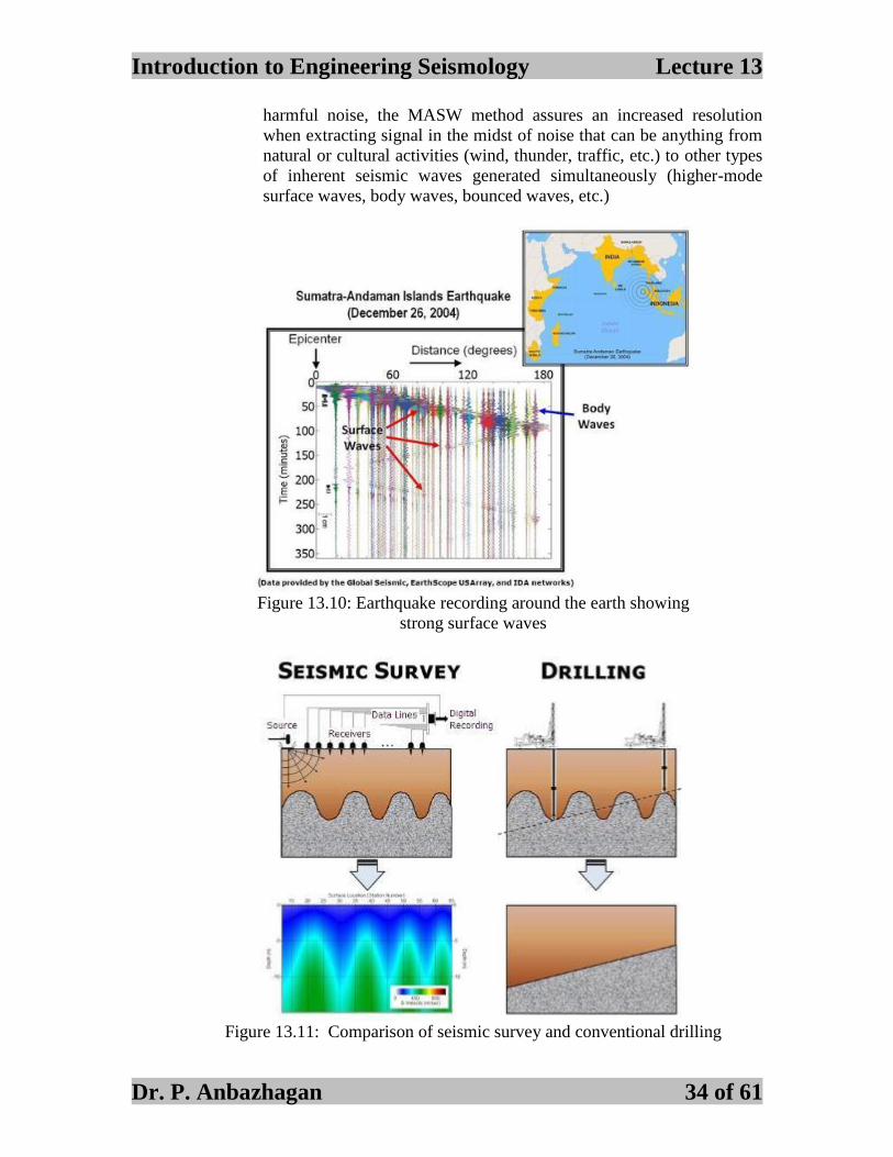
suffering from noise contamination (See Figure 13.10)
3. Because of an increased ability to discriminate useful signal from
Introduction to Engineering Seismology Lecture 13
Dr. P. Anbazhagan 34 of 61
harmful noise, the MASW method assures an increased resolution
when extracting signal in the midst of noise that can be anything from
natural or cultural activities (wind, thunder, traffic, etc.) to other types
of inherent seismic waves generated simultaneously (higher-mode
surface waves, body waves, bounced waves, etc.)
Figure 13.10: Earthquake recording around the earth showing
strong surface waves
Figure 13.11: Comparison of seismic survey and conventional drilling

Introduction to Engineering Seismology Lecture 13
Dr. P. Anbazhagan 35 of 61
4. In consequence, overall field procedure for data acquisition and
subsequent data-processing step becomes highly effective and
tolerant, rendering a non-expert method (Fig 13.11).
5. The multichannel seismic concept is analogous to resolution in
digital imaging technology (Figure 13.12). As the higher number
of bits available, a broader color resolution is achieved, whereas
the higher image resolution is achieved as more pixels are used to
capture the image. The concept of number of channels plays
similar roles to those by the bit and pixel concepts in delineating
the subsurface information.
Figure 13.12: An analogy of the seismic multichannel approach to digital imaging
concepts of number of bits and pixels
Overall Procedure of MASW Survey - The common procedure for (1-D, 2-
D, and 3-D) MASW surveys usually consist of three steps (Figure 13.13)
1. Data Acquisition - acquiring multichannel field records (commonly
called shot gathers in conventional seismic exploration)
2. Dispersion Analysis - extracting dispersion curves (one from each
record)
3. Inversion - back-calculating shear-wave velocity (Vs) variation with
depth (called 1-D Vs profile) that gives theoretical dispersion
curves closest to the extracted curves (one 1-D Vs profile from
each curve).

Introduction to Engineering Seismology Lecture 13
Dr. P. Anbazhagan 36 of 61
Figure 13.13: Common procedure for MASW surveys for 1-D, 2-D, and 3-D Vs
mapping.
Topic 23
Downhole Shear Wave Velocity
Steps involved in finding out the downhole shear wave velocity are:
1. Anchoring System
2. Automated Source
3. Polarized Wave

Introduction to Engineering Seismology Lecture 13
Dr. P. Anbazhagan 37 of 61
4. Downhole Vs
In the down-hole test, an impulse source is located on the ground surface
adjacent to the borehole. A single receiver that can be moved to different
depths, or a string of multiple receivers at predetermined depths, is fixed
against the walls of the borehole, and a single triggering receiver is located at
the energy source.
All receivers are connected to a high speed recording system so that their
output can be measured as a function of time. The objective of the downhole
test is to measure the travel times of the p and/or s-waves from the energy
source to the receivers.
By properly locating the receiver positions, a plot of travel time versus depth
can be generated. The slope of the travel-time curve at any depth represents the
wave propagation velocity at that depth.
With an SH-wave source, the down-hole test measures the velocity of waves
similar to those that carry most seismic energy to the ground surface. Because
the waves must travel through all materials between the impulse source and
receivers, the down-hole test allows detection of layers that can be hidden in
seismic refraction surveys.
Potential difficulties with down-hole tests and their interpretation can result
from disturbance of the soil during drilling of the borehole, casing and
borehole fluid effects, insufficient or excessively large impulse sources,
background noise effects.
The effects of material and radiation damping on wave forms can make
identification of s-wave arrivals difficult at depths greater than 30-60 m.
Topic 24
Automated Seismic Source
To improve upon the downhole testing program, an automatic seismic source
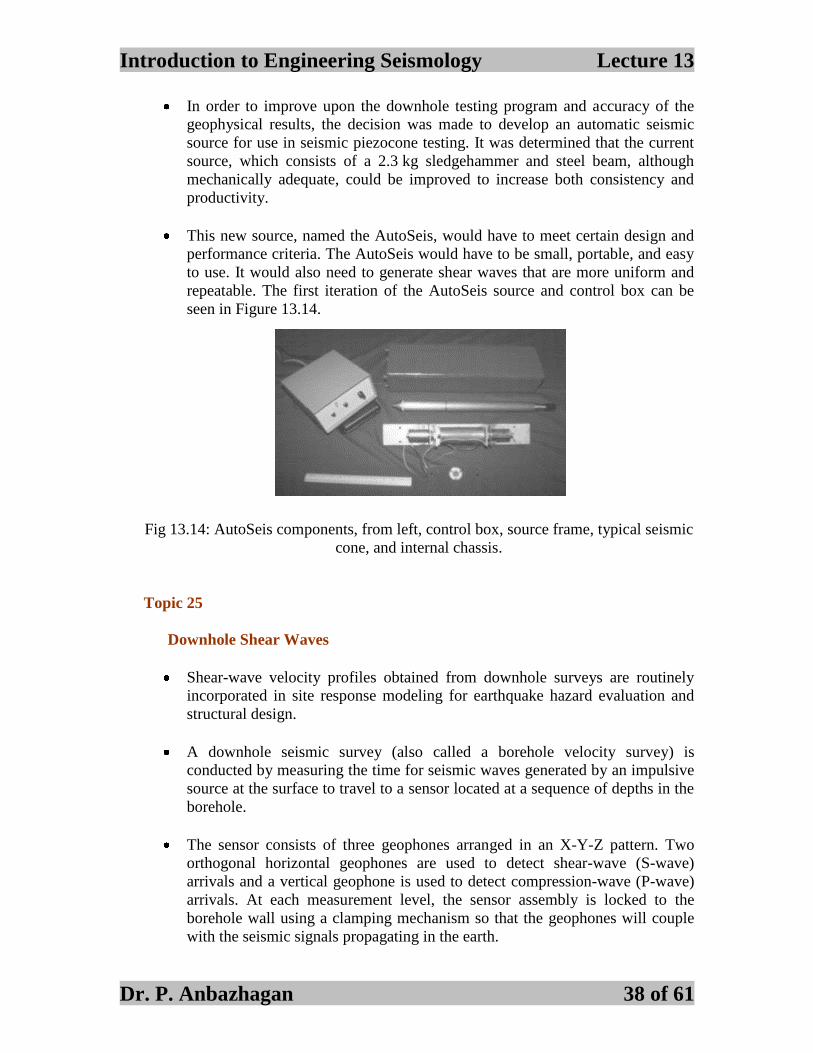
was developed for use in seismic piezocone testing. A new source, named the
AutoSeis, was initially tested at the national geotechnical experimentation site
in Spring Villa, Alabama and compared to available crosshole data to assess its
ability to meet the primary and secondary goals.
Later testing was conducted at two test sites in the Mid-America earthquake
region near Memphis. With reliable shear waves generated to a depth of 20 m,
the first iteration of the AutoSeis has proven successful and has provided the
necessary information for the design of an improved version.
Introduction to Engineering Seismology Lecture 13
Dr. P. Anbazhagan 38 of 61
In order to improve upon the downhole testing program and accuracy of the
geophysical results, the decision was made to develop an automatic seismic
source for use in seismic piezocone testing. It was determined that the current
source, which consists of a 2.3 kg sledgehammer and steel beam, although
mechanically adequate, could be improved to increase both consistency and
productivity.
This new source, named the AutoSeis, would have to meet certain design and
performance criteria. The AutoSeis would have to be small, portable, and easy
to use. It would also need to generate shear waves that are more uniform and
repeatable. The first iteration of the AutoSeis source and control box can be
seen in Figure 13.14.
Fig 13.14: AutoSeis components, from left, control box, source frame, typical seismic
cone, and internal chassis.
Topic 25
Downhole Shear Waves
Shear-wave velocity profiles obtained from downhole surveys are routinely
incorporated in site response modeling for earthquake hazard evaluation and
structural design.
A downhole seismic survey (also called a borehole velocity survey) is
conducted by measuring the time for seismic waves generated by an impulsive
source at the surface to travel to a sensor located at a sequence of depths in the
borehole.
The sensor consists of three geophones arranged in an X-Y-Z pattern. Two
orthogonal horizontal geophones are used to detect shear-wave (S-wave)
arrivals and a vertical geophone is used to detect compression-wave (P-wave)
arrivals. At each measurement level, the sensor assembly is locked to the
borehole wall using a clamping mechanism so that the geophones will couple
with the seismic signals propagating in the earth.
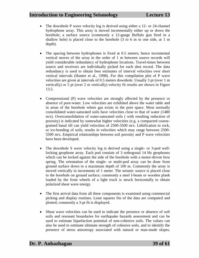
Introduction to Engineering Seismology Lecture 13
Dr. P. Anbazhagan 39 of 61
The downhole P wave velocity log is derived using either a 12- or 24-channel
hydrophone array. This array is moved incrementally either up or down the
borehole; a surface source (commonly a 12-gauge Buffalo gun fired in a
shallow hole) is placed close to the borehole (3 to 6 m to one side, at 1 m
depth).
The spacing between hydrophones is fixed at 0.5 meters; hence incremental
vertical moves of the array in the order of 1 m between source records will
yield considerable redundancy of hydrophone locations. Travel-times between
source and receivers are individually picked for each shot record. The data
redundancy is used to obtain best estimates of interval velocities over short
vertical intervals (Hunter et al., 1998). For this compilation plot of P wave
velocities are given at intervals of 0.5 meters downhole. Usually 3 pt (over 1 m
vertically) or 5 pt (over 2 m vertically) velocity fit results are shown in Figure
13.5.
Compressional (P) wave velocities are strongly affected by the presence or
absence of pore-water. Low velocities are exhibited above the water table and
in areas of the borehole where gas exists in the pore space. Most normally
consolidated water-saturated soils have velocities close to that of water (1480
m/s). Overconsolidation of water-saturated soils ( with resulting reduction of
porosity) is indicated by somewhat higher velocities (e.g. a compacted coarse-
grained basal till can yield velocities of 2500-3500 m/s. Lithification to rock,
or ice-bonding of soils, results in velocities which may range between 2500-
5500 m/s. Empirical relationships between soil porosity and P wave velocities
have been developed.
The downhole S wave velocity log is derived using a single- or 3-pod well-
locking geophone array. Each pod consists of 3 orthogonal 14 Hz geophones
which can be locked against the side of the borehole with a motor-driven bow
spring. The orientation of the single- or multi-pod array can be done from
ground surface down to a maximum depth of 100 m. Commonly the array is
moved vertically in increments of 1 meter. The seismic source is placed close
to the borehole on ground surface; commonly a steel I-beam or wooden plank
loaded by the front wheels of a light truck is struck horizontally to obtain
polarized shear wave energy.
The first arrival data from all three components is examined using commercial
picking and display routines. Least squares fits of the data are computed and
plotted; commonly a 3-pt fit is displayed.
Shear wave velocities can be used to indicate the presence or absence of soft
soils and resonant boundaries for earthquake hazards assessment and can be
used to estimate liquefaction potential of non-cohesive soils. The values can
also be used to estimate ultimate strength of cohesive soils, and to identify the
presence of stress anisotropy associated with natural or man-made slopes.

Introduction to Engineering Seismology Lecture 13
Dr. P. Anbazhagan 40 of 61
Emperical relationships between shear wave velocity and soil porosity have
been developed.
Fig 13.15: Downhole shear wave
Topic 26
Other Test used to Measure Shear wave velocity
The field tests or the in situ tests measure the dynamic soil properties without
altering the chemical, thermal or structural condition of the soil. The field test
can be broadly divided into two – low strain and large strain tests.
Low Strain Tests: The strain levels in these types of tests will be around
0.0001%. some of the important low strain tests are discussed below.
1. Seismic Reflection Test: This test is used to evaluate the wave propagation
velocity and the thickness of soil layers. The test setup will consist of a source
producing a seismic impulse and a receiver to identify the arrival of seismic
waves and the travel time from source to receiver is measured. Based on these
measurements, the thickness of soil layer can be evaluated.
-0.08
-0.06
-0.04
-0.02
0
0.02
0.04
0.06
0.08
0 50 100 150 200
Time (ms)
Am
pli
tud
e
-0.08
-0.06
-0.04
-0.02
0
0.02
0.04
0.06
0.08
0 50 100 150 200
Time (ms)
Am
pli
tud
e
-400
-300
-200
-100
0
100
200
300
400
500
-200 -150 -100 -50 0 50 100 150 200
-400
-300
-200
-100
0
100
200
300
400
500
-5 0 5 10 15 20
Time shift (ms)
Maximum crosscorrelation at t = 6.75 ms
Shear wave velocity = 155 m/s
Right Strike CROSSOVER Method
Left Strike
Shear Wave at 8.15 m
Shear Wave at 9.20 m CROSSCORRELATION

Introduction to Engineering Seismology Lecture 13
Dr. P. Anbazhagan 41 of 61
2. Seismic Refraction Test: This test will use the arrival time of the first
seismic wave at the receiver. Using the results obtained from this test the
delineation of major stratigraphic units is possible.
3. Suspension logging test: This test is used to measure the wave propagation
velocity and it is commonly used in petroleum industry. This is very effective
at higher depths (up to 2 km).
4. Steady state vibration test: In this test the wave propagation velocities are
measured from steady state vibration characteristics. However these tests can
be useful for determining the near surface shear wave velocity and they fail to
provide the details of highly variable soil profiles.
5. Seismic cross hole test: In seismic cross hole test the wave velocities are
measured using more than one bore hole (Fig. 13.16). In the simplest case two
bore holes are used – one with an impulse source and the other with a receiver
and both are kept at the same depth. The test is repeated at various depths to
get the soil profile. Generation of body waves dependent upon source type the
seismic wave generated could be P-, SV-, or SH body waves
Error!
Fig. 13.16: Seismic cross hole test (Courtesy www.microgeo.com)
Source
Hole Source
Hole
Receiver
No.1
Receiver
No.2

Introduction to Engineering Seismology Lecture 13
Dr. P. Anbazhagan 42 of 61
6. Seismic Down hole (up hole) test: This test is used to measure the travel time
of seismic waves from source to receiver. It is performed using a single
borehole. In seismic down hole test the receiver is kept at the ground surface
and the impulse source is kept at different depths. The up hole test is done
with receiver at the ground surface and the impulse source in the borehole.
This test is not effective for depths greater than 30 to 60 m.
Electrical Resistivity Tests - DC resistivity techniques, sometimes referred to as
electrical resistivity, electrical resistivity imaging or vertical electric sounding,
measure earth resistivity by driving a direct current (DC) signal into the ground
and measuring the resulting potentials (voltages) created in the earth. From that
data the electrical properties of the earth (the geoelectric section) can be derived
and thereby the geologic properties inferred.
Fig 13.17: schematic diagram showing the basic principle of DC resistivity
measurements.
Two short metallic stakes (electrodes) are driven about 1 foot into the earth to
apply the current to the ground. Two additional electrodes are used to measure the
earth voltage (or electrical potential) generated by the current (Fig. 3.17). Depth of
investigation is a function of the electrode spacing.
The greater the spacing between the outer current electrodes, the deeper the
electrical currents will flow in the earth, hence the greater the depth of exploration.
The depth of investigation is generally 20% to 40% of the outer electrode spacing,
depending on the earth resistivity structure.

Introduction to Engineering Seismology Lecture 13
Dr. P. Anbazhagan 43 of 61
Instrument readings (current and voltage) are generally reduced to "apparent
resistivity" values. The apparent resistivity is the resistivity of the homogeneous
half-space which would produce the observed instrument response for a given
electrode spacing. Apparent resistivity is a weighted average of soil resistivities
over the depth of investigation. For soundings a log-log plot of apparent resistivity
versus electrode separation is obtained. This is sometimes referred to as the
"sounding curve."
The resistivity data is then used to create a hypothetical model of the earth and it's
resistivity structure (geoelectric sections). Resistivity models are generally not
unique; i.e., a large number of earth models can produce the same observed data or
sounding curve. In general, resistivity methods determine the "conductance" of a
given stratigraphic layer or unit. The conductance is the product of the resistivity
and the thickness of a unit. Hence that layer could be thinner and more conductive
or thicker and less conductive, and produce essentially the same results. Because
of these constraints on the model, borehole data or assumed unit resistivities can
greatly enhance the interpretation.
The end product from a DC resistivity survey is generally a "geoelectric" cross
section (model) showing thicknesses and resistivities of all the geoelectric units or
layers. If borehole data or a conceptual geologic model is available, then a
geologic identity can be assigned to the geoelectric units. A two-dimensional
geoelectric section may be made up of a series of one-dimensional soundings
joined together to form a two-dimensional section, or it may be a continual two-
dimensional cross section. The type of section produced depends on the
acquisition parameters and the type of processing applied to the data.
Topic 27
Ground Penetration Radar
Introduction
Ground penetrating radar (GPR) is a geophysical technique to detect and identify
structures, either natural or man-made, below the ground surface.GPR is a
nondestructive method that produces a continuous cross-sectional profile or
record of subsurface features, without drilling, probing, or digging.
GPR profiles are used for evaluating the location and depth of buried objects and
to investigate the presence and continuity of natural subsurface conditions and
features. GPR is a nondestructive and environmentally safe method to detect,
locate and map subsurface features. The fundamental principle of operation is the
same as that used to detect aircraft overhead, but with GPR that antennas are
moved over the surface rather than rotating about a fixed point.

Introduction to Engineering Seismology Lecture 13
Dr. P. Anbazhagan 44 of 61
The radar technique was first proposed during the first decades of the 20th
century but was not made truly, practically, functional until the military demands
of World War II pushed the development forward. After the war commercial
vehicle tracking radars for ships, airports etc. were quickly developed. Some
experiments using pulsed radars for mapping of glaciers were also reported in the
first decades of the century, but no really usable equipment similar to the GPR of
today were available until the early 70s.
We believe it's fair to say that up until the mid 70s all equipment as well as the
services performed was related to scientific studies. In the early 70s the first
commercial GPR equipment was introduced. These first GPR instruments were
extremely expensive, large, analogue and difficult to operate. As with many other
techniques the "digital revolution" changed the scene. During the 80s true digital,
smaller and more efficient GPR units appeared on the market. The 90s was a
decade when the personal computers as wells as miniaturized electronics changed
the GPR products. From now on there were one-man systems as well as relatively
easy to use systems available.
From 2000 onwards people started to see dedicated systems, designed for special
applications, with simplified man-to-machine interfaces. Improved and user-
friendly software with semi-automatic processing of data has also helped to make
ground penetrating radar become a technique usable for the technically skilled
common man.
Radar Principal
Radar is short for Radio Detection and Ranging, so it's quite clear what it is all
about: detection of a target and determination of its distance from the radar
antenna. In general radar systems determine not only the distance but also the
direction or location of the target. Both conventional radars and GPR use the same
principle of traveling and reflected electromagnetic waves although the ways the
waves are generated and treated are completely different.
A radar pulse is emitted by the transmitter antenna is partly reflected and partly
transmitted when it meets with an electrical discontinuity in the ground, that is an
interface at which there are a change in electromagnetic wave impedance or in
other words a change in electrical properties. If the time for the pulse to go to the
reflector and back again to the receiver antenna is measured, the location of the
reflector in the ground can be decided, if the velocity of the pulse is known. It can
be seen from Figure 13.18 clearly the interfaces as layers result in a layer in the
radargram, whereas objects form so called hyperbolas.
Theories of electromagnetic and seismic (elastic) wave propagation are similar in
many respects. Both waves propagate with finite velocities that depend upon the
material properties, and both are reflected and refracted based on local changes.
The propagation of electromagnetic pulse depends upon dielectric properties of

Introduction to Engineering Seismology Lecture 13
Dr. P. Anbazhagan 45 of 61
the material. This method is not suitable in high conductivity environments such
as soils with saline water, as electromagnetic fields diffuse into the ground. An
approximate value of electromagnetic parameters of typical soils and rocks are
provided in the Table 13.7.
Figure 13.18: Basic principle of radar measurement
Table 13.7: Electromagnetic Parameters of Various Types of Rocks and Soils (Morey,
1974; Ulriksen, 1983)
Material Conductivity,
(mho/m or S/m)
Relative
permittivity, K
Attenuation,
(dB/m)
Velocity, C
(cm/ns)
Air 0 1 0 30
Fresh water 10-3 81 0.18 3.3
Sea water 4.0 81 103 3.3
Granite (dry) 10-8 5 10-5 13
Granite (wet) 10-3 7 0.6 11
Basalt (wet) 10-2 8 5.6 11
Shale (wet) 10-1 7 45 11
Sandstone(wet) 4 × 10⁻² 6 24 12
Limestone (wet) 2.5 × 10⁻² 8 14 11
Sandy soil (dry) 1.5 × 10⁻⁴ 3 0.14 17
Sandy soil (wet) 7 × 10⁻³ 25 2.3 6
Clayey soil (dry) 2.5 × 10⁻⁴ 3 0.28 17
Clayey soil (wet) 5 × 10⁻² 15 20 7.8
Introduction to Engineering Seismology Lecture 13
Dr. P. Anbazhagan 46 of 61
Topic 28
Comparison of GPR from Other Non Destructive Methods
Seismic methods
Comparisons are often done is between seismic methods and GPR. Now what is
the difference between these two methods? The resulting data looks very similar
There are however a few fundamental things which distinguish the two techniques
from each other:
1. In seismic method, the reflection of the wave is caused by changes in the
density of the material under investigation. In GPR the reflections are caused
by changes in the electric properties, primarily in the dielectric constant ε.
2. Seismic methods require a very good physical contact between the
receiving/transmitting elements and the ground.
3. Seismic method is at least 10 times more expensive than GPR per meter of
profile.
4. In GPR the velocity of the media usually never change more than 50% and
that would be a rather extreme case, on a certain site. In seismic velocity
contrasts can be much larger. This is because variations in density are much
stronger than variations in the dielectric constant.
5. GPR shows much more detail than seismic, in other words, the resolution for
GPR is higher.
6. Seismic methods work very well in clay where GPR is almost useless. It also
penetrates kilometers instead of meters as for GPR.
Ultrasonic methods
Much of what was said about seismic is also true for ultrasonic since they are both
acoustic methods, only the frequency differs. However the instrumentation is
different and that makes a separate comparison valid:
1. In ultrasonics the frequency is often high enough to make mm resolution
possible e.g. in medicine.
2. The contact with ground/media has to be so good that the sensors are often
glued to the material one wants to investigate, or a contact gel is used.
Metal detectors/cover meters
Cover meters are types of instruments used for detection of rebar in concrete and
metal detectors is probably familiar to everyone. Obviously these instruments
only detect metal, there are, however, a few more distinguishing characteristics:
1. Cover meters can never see through a wire mesh, anything below a first layer
would be hidden. High-resolution radar sees trough a wire mesh and can
detect both metallic and non-metallic objects under it.

Introduction to Engineering Seismology Lecture 13
Dr. P. Anbazhagan 47 of 61
2. Cover meters are based on an assumption of a certain diameter of the rebars.
This means that if two rebars are too close the instrument will become very
uncertain.
3. Metal detectors can be made very easy to use and also tuned to detect very
small pieces of metal, smaller than GPR can resolve.
EM-locators
EM-locators are used locate cables and metal pipes. They can be used both in
active and passive mode, active meaning when the transmitter of the EM-locator
is connected to the target. In practice the active mode is much preferred and
people tend to not using the passive mode. When the active mode is possible,
these instruments are easy to use and reliable. GPR is seldom used in these cases.
Still there are many cases where GPR is more favorable:
1. GPR detects both metallic and non-metallic targets; an EM-detector is only
capable of locating the metal ones.
2. The active mode requires the pipe, cable or tracer wire to be unbroken. For
GPR this doesn‘t matter.
3. GPR can pinpoint many targets at one swat, when using an EM-locator you
concentrate on one at a time, normally.
X-ray
No need to argue, X-ray is probably the most revealing NDT method. However it
is very expensive, not only due to the complex security measures necessary
during its application it's also quite slow and cumbersome.
Topic 29
The Basic Radar System
A radar system consist of
1. A control unit, which generates the control signals for the receiver and
transmitter antenna electronics, keeps track of the distance along the profile
and buffers data from receiver.
2. Transmitter antenna electronics, which generates impulses or steps, fed to
the transmitting antenna.
3. Receiver antenna electronics, which takes care of the incoming signals for
digitisation and storage.
4. Transmitter and Receiver antenna elements, bi-static. These can either be
two separate units or mounted together in a box.
5. A recording facility to store and display data. Most often this would be a
laptop or a dedicated monitor.
6. An encoder to position and trigger the measurements, most often a survey
wheel or hip-chain, sometimes combined with GPS.
Introduction to Engineering Seismology Lecture 13
Dr. P. Anbazhagan 48 of 61
GPR used for - As said before, only the imagination is setting the real limits for
what can be done with GPR. In this section we're listing a few application areas in
which GPR have been used previously. This list of assessments and analysis is not
complete and new applications are added all the time.
Archaeology Borehole Bridge deck Building assessment
Forensic Remote sensing Geophysical Rail track
Contaminated soil Utility Road Asphalt thickness
Trunk condition Snow thickness Concrete Moisture assessment
Soil classification Earth dam Tunnel detection Fault study
Topic 30
Grids for Site characterization
Site characterization done to the areas are divided into cells by a grid system for
estimating the effects of site conditions by assigning representative soil profiles at
the centre of each grid.
Site response analyses were conducted for each grid using the acceleration spectra
compatible simulated earthquake time histories obtained for each grid separately
based on the seismic hazard study.
Pilot areas were divided into grids to evaluate the representative parameters for
each grid by defining hypothetical boreholes located at the centre of the grids. A
hypothetical borehole should be an idealized borehole, which will be the most
representative for the soil conditions in the specific grid. In an ideal project, new
site investigations might be conducted, almost in the centre of each of the grids.
There are basically two reasons behind the grid approach adopted for evaluating
and interpreting the effects of site conditions on the ground motion at the free
field.
1. To utilize all the available data in each grid in order to have more
comprehensive and reliable information about the soil profile;
2. To eliminate the effects of different distances among boreholes or site
investigation points during the GIS mapping.
The results obtained were mapped using GIS techniques by applying linear
interpolation among the grid points, thus enabling a smooth transition of the
selected parameters. Soft transition boundaries are preferred to show the variation
of the mapped parameters.

Introduction to Engineering Seismology Lecture 13
Dr. P. Anbazhagan 49 of 61
Topic 31
Interpolation of non-filled grids and hypothetical boreholes
The pilot areas were divided into cells by a grid system, if there are no boreholes
or in-situ tests conducted in the outer grids, and then the boundaries of the both
regions are modified as shown in the following maps for microzonation study to
avoid the need for additional extrapolation that may not be very reliable.
Interpolation of data to fill empty grid points has been carried out very carefully
and was omitted for doubtful cases as well as for cases where extrapolation of
borehole data would have been needed.
A hypothetical borehole should be an idealized borehole, which will be the most
representative for the soil conditions in the specific grid. In an ideal project, new
site investigations might be conducted, almost in the centre of each of the grids.
The hypothetical borehole was introduced for each grid as the soil profile,
including the extension up to competent layer. In case of mixed layers, the softer
layer has been chosen as the representative one.
Topic 32
Site Classification and 30m Concept
Seismic hazard analysis gives seismic hazard parameters at rock level. But
damages due to seismic activities depend upon the site specific properties
subsurface materials within a km from surface. Site characterization is process of
classifying region/ site considering average subsurface material properties.
Classification of individual sites based on the properties is a more direct indicator
of local site effects.
Seismic site classification systems are inevitably reflected in modern seismic codal
provisions to account for site effects. Recent modern seismic codes in America,
Europe, Japan and worldwide [International building code (IBC 2009), Unified
Building code (UBC 97), National Earthquake Hazards Reduction Program
(NEHRP, BSSC, 2001) and Euro code 8, 2007] have produced numerous valuable
information based on experimental and theoretical results.
In engineering site investigation, 30 m is a typical depth of borings and detailed
site characterizations. Therefore, most of the site-effect studies in earthquake
ground motions are based on the properties in the upper 30 m.
For instance, Boore et al. (1993, 1994) based their regressions for ground motions
on average shear velocity in the upper 30 m. Borcherdt (1992, 1994) and Martin

Introduction to Engineering Seismology Lecture 13
Dr. P. Anbazhagan 50 of 61
and Dobry (1994) recommended that design of structures be based on these
properties. The 30m average concept is widely used for the seismic
Microzonation by considering experimental data from geotechnical and
geophysical testing.
The site classes are defined in terms of shear velocity to a depth of 30m, denoted
by Vs30
, if no measurements of Vs to 30 m are feasible corresponding limits in
terms of standard penetration resistance (N) and undrained shear strength ( Su )
(Borcherdt, 1994).
Site classification is followed in modern seismic codes to arrive design spectrum
and some extent to represents site and induced effects of the site during
earthquakes. This will also help to delineate sites for detailed analysis.
The geotechnical parameters used to define the site class are based on the upper
100 ft (30 480 mm) of the site profile. Profiles containing distinctly different soil
and rock layers shall be subdivided into those layers designated by a numbers that
ranges from 1 to n at the bottom where there are a total of n distinct layers in the
upper 100 ft (30 480 mm). The symbol/then refers to any one of the layers
between 1 and n
Where n
i
id1
is equal to 100 ft (30 480 mm)
Shear wave velocity
Where vsi = the shear wave velocity in ft/sec or m/s
di = the thickness of any layer (between o and 100 ft [30 480 mm])
Standard Penetration Resistance
Where Ni and di in above equation are for cohesionless soil, cohesive soil, and
rock layers.
For cohesionless soil layers
n
i si
i
n
i
i
s
v
d
d
v
1
1
n
i i
i
n
i
i
N
d
d
N
1
1
m
i i
i
sch
N
d
dN
1
(13.9)
(13.10)
(13.11)
Introduction to Engineering Seismology Lecture 13
Dr. P. Anbazhagan 51 of 61
Where Ni and di in above equation are for cohesionless soil layers only
and s
m
i
i dd1
ds = the total thickness of cohesionless soil layers in the top 100 ft (30 480
mm)
m = The number of cohesionless soil layers in the top 100 feet (30 480
mm).
Ni = The Standard Penetration Resistance determined in accordance with ASTM D
1586, as directly measured in the field without corrections, and shall not be taken
greater than 100 blows/ft. where refusal is met for rock layer, Ni shall be taken as
100 blows/ft
Undrained Shear Strength
Where c
k
i
i dd1
dc = the total thickness of cohesive soil layers in the top 100 ft (30 480 mm)
sui = The undrained shear strength in psf (kPa), not to exceed 5,000 psf (240 kPa),
ASTM D 2166 or D 2850.
chN for cohesionless soil layers (PI<20) in the top 100 ft (30 m) and average us
for cohesive soil layers (PI>20) in the top 100 ft (30 m)
PI = the plasticity index, ASTM D 4318.
Topic 33
Site Class Definitions – International Building Code
Based on the site soil properties, the site shall be classified as Site Class A, B, C,
D, E or F in accordance with Table 13.8. When the soil properties are not known
in sufficient detail to determine the site class, Site Class D shall be used unless the
building official or geotechnical data determines that Site Class E or F soil is
likely to be present at the site.
k
i ui
i
cu
S
d
ds
1
(13.12)

Introduction to Engineering Seismology Lecture 13
Dr. P. Anbazhagan 52 of 61
Table 13.8: Site Class Definitions as per International Building Code (IBC, 2009)
Site
Classification
Description
Average Properties in Top 30m
Shear wave
velocity (m/s)
SPT N
(blows/300mm)
Undrained
Shear Strength
su (kPa)
A Hard Rock >1500 NA NA
B Rock 750-1500 NA NA
C Very dense soil
and Soft rock
360-750 >50 >100
D Stiff soil 180-360 15-50 50-100
E
Soft Soil <180 <15 <50
Plus any profile with more than 3m of soil having the
following characteristics:
Plasticity Index, PI >20%
Moisture content, w ≥ 40%
Undrained Shear strength, Su <25kPa
F Any profile containing soils with one or more of the following
characteristics
Soil vulnerable to potential collapse under seismic loading e.g.
liquefiable soils, quick and highly sensitive clay, collapsible weakly
cemented soils.
Peats and/or highly organic clays (H>8m of peat and/or highly organic
clay)
Very high plasticity clays (H>8m with PI>75%)
Very thick soft/medium stiff clays (H>36m)
Where the soil properties are not known in sufficient detail to determine the site calss in
accordance with below, it shall be permitted to assume Site class D unless the authority
having jurisdiction determines that site class E or F could apply at the site or in the event
that Site Class E or F is established by geotechnical data
Site Class definitions. The Site Classes are defined as follows:
A Hard rock with measured shear wave velocity, sv >5,000 ft/sec (1500 m/s)
B Rock with 2,500 ft/sec < sv ≤ 5,000 ft/sec (760 m/s < sv ≤ 1,500 m/s)
C Very dense soil and soft rock with 1,200 ft/sec < sv ≤ 2,500 ft/sec (360 m/s < sv ≤
760 m/s) or with either N >50 or us > 2,000 psf (100 kPa)
D Stiff soil with 600 ft/sec ≤ sv ≤ 1,200 ft/sec (180 m/s < sv ≤ 360 m/s) or with either
15 ≤ N >50 or 1,000 psf ≤ us ≤ 2,000 psf (50 kPa ≤ us ≤100 kPa)
E A soil profile with sv < 600 ft/sec (180 m/s) or with either
N <15, us < 1,000 psf, or any profile with more than 10 ft (3 m) of soft clay
defined as soil with PI>20, w≥40 percent, and su<500 psf (25 kPa)
F Soils requiring site-specific evaluations:
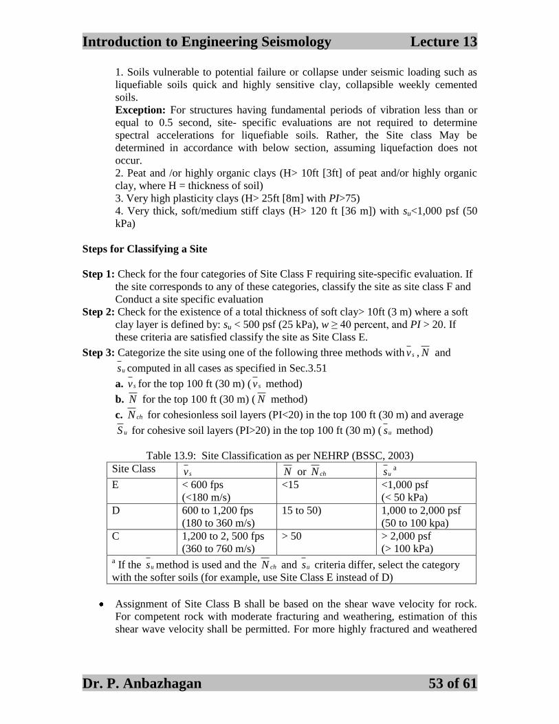
Introduction to Engineering Seismology Lecture 13
Dr. P. Anbazhagan 53 of 61
1. Soils vulnerable to potential failure or collapse under seismic loading such as
liquefiable soils quick and highly sensitive clay, collapsible weekly cemented
soils.
Exception: For structures having fundamental periods of vibration less than or
equal to 0.5 second, site- specific evaluations are not required to determine
spectral accelerations for liquefiable soils. Rather, the Site class May be
determined in accordance with below section, assuming liquefaction does not
occur.
2. Peat and /or highly organic clays (H> 10ft [3ft] of peat and/or highly organic
clay, where H = thickness of soil)
3. Very high plasticity clays (H> 25ft [8m] with PI>75)
4. Very thick, soft/medium stiff clays (H> 120 ft [36 m]) with su<1,000 psf (50
kPa)
Steps for Classifying a Site
Step 1: Check for the four categories of Site Class F requiring site-specific evaluation. If
the site corresponds to any of these categories, classify the site as site class F and
Conduct a site specific evaluation
Step 2: Check for the existence of a total thickness of soft clay> 10ft (3 m) where a soft
clay layer is defined by: su < 500 psf (25 kPa), w ≥ 40 percent, and PI > 20. If
these criteria are satisfied classify the site as Site Class E.
Step 3: Categorize the site using one of the following three methods with sv , N and
us computed in all cases as specified in Sec.3.51
a. sv for the top 100 ft (30 m) ( sv method)
b. N for the top 100 ft (30 m) ( N method)
c. chN for cohesionless soil layers (PI<20) in the top 100 ft (30 m) and average
uS for cohesive soil layers (PI>20) in the top 100 ft (30 m) ( us method)
Table 13.9: Site Classification as per NEHRP (BSSC, 2003)
Site Class sv N or chN us
a
E < 600 fps
(<180 m/s)
<15 <1,000 psf
(< 50 kPa)
D 600 to 1,200 fps
(180 to 360 m/s)
15 to 50) 1,000 to 2,000 psf
(50 to 100 kpa)
C 1,200 to 2, 500 fps
(360 to 760 m/s)
> 50 > 2,000 psf
(> 100 kPa) a If the us method is used and the chN and us criteria differ, select the category
with the softer soils (for example, use Site Class E instead of D)
Assignment of Site Class B shall be based on the shear wave velocity for rock.
For competent rock with moderate fracturing and weathering, estimation of this
shear wave velocity shall be permitted. For more highly fractured and weathered

Introduction to Engineering Seismology Lecture 13
Dr. P. Anbazhagan 54 of 61
rock, the shear wave velocity shall be directly measured or the site shall be
assigned to Site Class C.
Assignment of Site Class A shall be supported by either shear wave velocity
measurements on site or shear wave velocity measurements on profiles of the
same rock type in the same formation with an equal or greater degree of
weathering and Fracturing. Where hard rock conditions are known to be
continuous to a depth of 100 ft (30 m), surficial shear wave velocity
measurements may be extrapolated to assess sv .
Site Classes A and B shall not be used where there is more than 10 ft (3 m) of soil
between the rock surface and the bottom of the spread footing or mat foundation.
Topic 34
Site Class Definitions – European Standard
Further guidance concerning ground investigation and classification is given in
EN 1998-5:2004, 4.2.
The construction site and the nature of the supporting ground should normally be
free from risks of ground rupture, slope instability and permanent settlements
caused by liquefaction or densification in the event of an earthquake. The
possibility of occurrence of such phenomena shall be investigated in accordance
with EN 1998- 5:2004, Section 4.
Depending on the importance class of the structure and the particular conditions
of the project, ground investigations and/or geological studies should be
performed to determine the seismic action.
Identification of ground types
Ground types A, B, C, D, and E, described by the stratigraphic profiles and
parameters given in Table 3.1 and described hereafter, may be used to account for
the influence of local ground conditions on the seismic action. This may also be
done by additionally taking into account the influence of deep geology on the
seismic action.
Th e s ite s h ou ld be cla s s ified a ccord in g to th e va lu e of th e a vera ge
s h ea r wa ve velocity, vs,30, if th is is a va ila b le. Oth erwis e th e va lu e of
NSPT s h ou ld be u s ed .
The average shear wave velocity vs,30 should be computed in accordance with the
following expression:
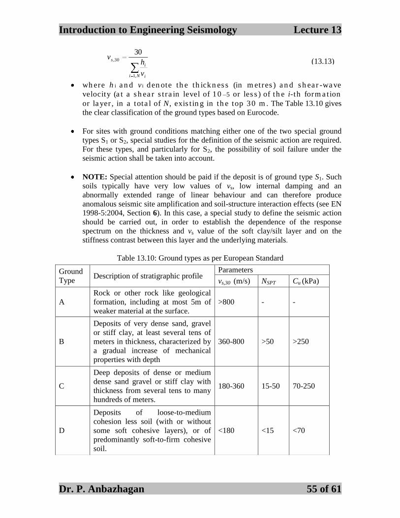
Introduction to Engineering Seismology Lecture 13
Dr. P. Anbazhagan 55 of 61
Ni i
i
s
v
hv
,1
30,
30
wh ere h i a n d v i den ote th e th ickn es s (in m etres ) a n d s h ea r -wa ve
velocity (a t a s h ea r s t ra in level of 10 –5 or les s ) of th e i-th form a t ion
or la yer , in a tota l of N, exis t in g in th e top 30 m . The Table 13.10 gives
the clear classification of the ground types based on Eurocode.
For sites with ground conditions matching either one of the two special ground
types S1 or S2, special studies for the definition of the seismic action are required.
For these types, and particularly for S2, the possibility of soil failure under the
seismic action shall be taken into account.
NOTE: Special attention should be paid if the deposit is of ground type S1. Such
soils typically have very low values of vs, low internal damping and an
abnormally extended range of linear behaviour and can therefore produce
anomalous seismic site amplification and soil-structure interaction effects (see EN
1998-5:2004, Section 6). In this case, a special study to define the seismic action
should be carried out, in order to establish the dependence of the response
spectrum on the thickness and vs value of the soft clay/silt layer and on the
stiffness contrast between this layer and the underlying materials.
Table 13.10: Ground types as per European Standard
Ground
Type Description of stratigraphic profile
Parameters
vs,30 (m/s) NSPT Cu (kPa)
A
Rock or other rock like geological
formation, including at most 5m of
weaker material at the surface.
>800 - -
B
Deposits of very dense sand, gravel
or stiff clay, at least several tens of
meters in thickness, characterized by
a gradual increase of mechanical
properties with depth
360-800 >50 >250
C
Deep deposits of dense or medium
dense sand gravel or stiff clay with
thickness from several tens to many
hundreds of meters.
180-360 15-50 70-250
D
Deposits of loose-to-medium
cohesion less soil (with or without
some soft cohesive layers), or of
predominantly soft-to-firm cohesive
soil.
<180 <15 <70
(13.13)

Introduction to Engineering Seismology Lecture 13
Dr. P. Anbazhagan 56 of 61
Topic 35
Comparison of seismic site classification
Seismic ground response characteristics, defined generally as ―site effects‖, are
inevitably incorporated in modern seismic code provisions in many countries.
However, the definitions of site classes in different codes are not consistent. The
summary of site classes adopted in Table 13.11 shows the summary of site classes
adopted in National Earthquake Hazards Reduction Program (NEHRP) (BSSC,
2001), International Building Code (IBC, 2009) or Uniform Building Code (UBC,
1997) and Eurocode 8 (2007). In order to avoid confusion of detailed
specifications, only key information is given in Table 13.10 for direct comparison.
Table 13.11: Site classification system given in modern seismic codes
Site
Class
Generalized
Description
NEHRP IBC 2009/ Eurocode 8 (2007)
$
(BSSC,2001) UBC1997
N30 Vs30
N30 Vs30
N30 Vs30
A Hard rock N/A >1500 N/A >1524 N/A N/A
B Rock N/A 760-
1500 N/A
762-
1524 >800
C
Very dense
soil and
soft rock
> 50 360-760 > 50 366-762 >50 360-800
D
Dense to
medium
soils
15-50 180-360 15-50 183-366 15 - 50 180 -
360
E
A soil profile consisting of a surface
alluvium layer with Vs values of
type C or D and thickness varying
between about 5 m and 20 m,
underlain by stiffer material with Vs
> 800 m/s.
S1
Deposits consisting, or containing a
layer at least 10 m thick, of soft
clays/silts with a high plasticity
index (PI > 40) and high water
content
<100
(indicative) - 10 to 20
S2
Deposits of liquefiable soils, of
sensitive clays, or any other soil
profile not included in types A – E or
S1
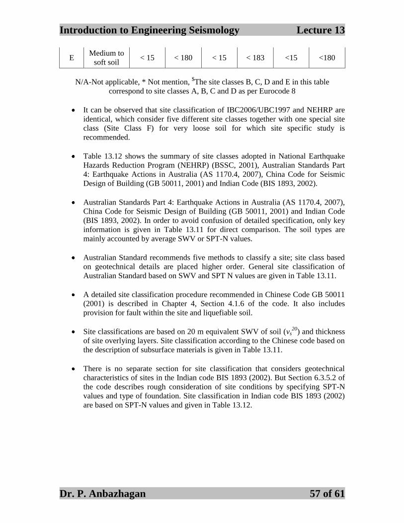
Introduction to Engineering Seismology Lecture 13
Dr. P. Anbazhagan 57 of 61
E Medium to
soft soil < 15 < 180 < 15 < 183 <15 <180
N/A-Not applicable, * Not mention, $The site classes B, C, D and E in this table
correspond to site classes A, B, C and D as per Eurocode 8
It can be observed that site classification of IBC2006/UBC1997 and NEHRP are
identical, which consider five different site classes together with one special site
class (Site Class F) for very loose soil for which site specific study is
recommended.
Table 13.12 shows the summary of site classes adopted in National Earthquake
Hazards Reduction Program (NEHRP) (BSSC, 2001), Australian Standards Part
4: Earthquake Actions in Australia (AS 1170.4, 2007), China Code for Seismic
Design of Building (GB 50011, 2001) and Indian Code (BIS 1893, 2002).
Australian Standards Part 4: Earthquake Actions in Australia (AS 1170.4, 2007),
China Code for Seismic Design of Building (GB 50011, 2001) and Indian Code
(BIS 1893, 2002). In order to avoid confusion of detailed specification, only key
information is given in Table 13.11 for direct comparison. The soil types are
mainly accounted by average SWV or SPT-N values.
Australian Standard recommends five methods to classify a site; site class based
on geotechnical details are placed higher order. General site classification of
Australian Standard based on SWV and SPT N values are given in Table 13.11.
A detailed site classification procedure recommended in Chinese Code GB 50011
(2001) is described in Chapter 4, Section 4.1.6 of the code. It also includes
provision for fault within the site and liquefiable soil.
Site classifications are based on 20 m equivalent SWV of soil (vs20
) and thickness
of site overlying layers. Site classification according to the Chinese code based on
the description of subsurface materials is given in Table 13.11.
There is no separate section for site classification that considers geotechnical
characteristics of sites in the Indian code BIS 1893 (2002). But Section 6.3.5.2 of
the code describes rough consideration of site conditions by specifying SPT-N
values and type of foundation. Site classification in Indian code BIS 1893 (2002)
are based on SPT-N values and given in Table 13.12.
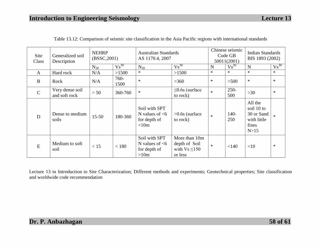
Introduction to Engineering Seismology Lecture 13
Dr. P. Anbazhagan 58 of 61
Table 13.12: Comparison of seismic site classification in the Asia Pacific regions with international standards
Lecture 13 in Introduction to Site Characterization; Different methods and experiments; Geotechnical properties; Site classification
and worldwide code recommendation
Site
Class
Generalized soil
Description
NEHRP
(BSSC,2001)
Australian Standards
AS 1170.4, 2007
Chinese seismic
Code GB
50011(2001)
Indian Standards
BIS 1893 (2002)
N30 Vs30
N30 Vs30
N Vs20
N Vs30
A Hard rock N/A >1500 * >1500 * * * *
B Rock N/A 760-
1500 * >360 * >500 * *
C Very dense soil
and soft rock > 50 360-760 *
≤0.6s (surface
to rock) *
250-
500 >30 *
D Dense to medium
soils 15-50 180-360
Soil with SPT
N values of <6
for depth of
<10m
>0.6s (surface
to rock) *
140-
250
All the
soil 10 to
30 or Sand
with little
fines
N>15
*
E Medium to soft
soil < 15 < 180
Soil with SPT
N values of <6
for depth of
>10m
More than 10m
depth of Soil
with Vs ≤150
or less
* <140 <10 *