Introduction to Electrical Engineering_Er. J. P. Navani and Er. S. Sapra

Scilab Textbook Companion forIntroduction to Electrical Engineeringby Er. J. P. Navani and Er. S. Sapra1

Created byMohd Anwar

B.TechElectronics Engineering

Roorkee Institute of TechnologyCollege Teacher

Mr. Mohd RizwanCross-Checked byK. V. P. Pradeep

May 8, 2014

1Funded by a grant from the National Mission on Education through ICT,http://spoken-tutorial.org/NMEICT-Intro. This Textbook Companion and Scilabcodes written in it can be downloaded from the ”Textbook Companion Project”section at the website http://scilab.in

Book Description

Title: Introduction to Electrical Engineering

Author: Er. J. P. Navani and Er. S. Sapra

Publisher: S. Chand & Company, New Delhi

Edition: 1

Year: 2013

ISBN: 81-219-9759-3

1

Scilab numbering policy used in this document and the relation to theabove book.

Exa Example (Solved example)

Eqn Equation (Particular equation of the above book)

AP Appendix to Example(Scilab Code that is an Appednix to a particularExample of the above book)

For example, Exa 3.51 means solved example 3.51 of this book. Sec 2.3 meansa scilab code whose theory is explained in Section 2.3 of the book.

2

Contents

List of Scilab Codes 4

1 D C Circuit Analysis 10

2 Network Theorems 33

3 AC fundamental 55

4 Three Phase AC Circuits 64

5 Three Phase AC Circuits 88

6 Measuring Instruments 101

8 Magnetic Circuits 108

9 Single Phase Transformer 120

10 D C Machines 138

11 Induction Motors 153

3

List of Scilab Codes

Exa 1.1 Current in each element . . . . . . . . . . . . . . . . . 10Exa 1.2 Current in each branch . . . . . . . . . . . . . . . . . 11Exa 1.3 Voltage source to current source . . . . . . . . . . . . 12Exa 1.4 Value of current . . . . . . . . . . . . . . . . . . . . . 12Exa 1.5 Value of I1 and I2 . . . . . . . . . . . . . . . . . . . . 13Exa 1.6 Current through each battery and load current . . . . 14Exa 1.7 Mesh analysis . . . . . . . . . . . . . . . . . . . . . . . 14Exa 1.8 Current in 6 ohm resistor . . . . . . . . . . . . . . . . 15Exa 1.9 Current in each element . . . . . . . . . . . . . . . . . 16Exa 1.10 Value of R3 and R4 . . . . . . . . . . . . . . . . . . . 17Exa 1.11 Current through each resistor . . . . . . . . . . . . . . 18Exa 1.12 Current in each branch . . . . . . . . . . . . . . . . . 19Exa 1.13 Voltage at node 1 and 2 . . . . . . . . . . . . . . . . . 20Exa 1.14 Current I1 and I2 . . . . . . . . . . . . . . . . . . . . 21Exa 1.15 Current I1 and I2 . . . . . . . . . . . . . . . . . . . . 22Exa 1.16 Current in resistor R1 . . . . . . . . . . . . . . . . . . 22Exa 1.17 Current in 10 ohm resistor . . . . . . . . . . . . . . . 23Exa 1.19 Current in each branch . . . . . . . . . . . . . . . . . 24Exa 1.20 Current in 8 ohm resistor . . . . . . . . . . . . . . . . 25Exa 1.21 Current drawn from the source . . . . . . . . . . . . . 26Exa 1.22 Current in all branch . . . . . . . . . . . . . . . . . . 27Exa 1.23 Current and voltage across 2 ohm resistor . . . . . . . 28Exa 1.24 Voltage across 6 ohm resistor . . . . . . . . . . . . . . 29Exa 1.25 Resistance between point B and C . . . . . . . . . . . 30Exa 1.26 Voltage across R1 and R2 . . . . . . . . . . . . . . . . 31Exa 1.27 Current I1 and I2 . . . . . . . . . . . . . . . . . . . . 31Exa 2.1 Current through load resistance . . . . . . . . . . . . . 33Exa 2.2 Value of current across 12 ohm . . . . . . . . . . . . . 34

4

Exa 2.3 Value of current across 12 ohm . . . . . . . . . . . . . 34Exa 2.4 Load resistor . . . . . . . . . . . . . . . . . . . . . . . 35Exa 2.5 Current across 4 ohm resistor . . . . . . . . . . . . . . 35Exa 2.6 Current in branch AB . . . . . . . . . . . . . . . . . . 36Exa 2.7 Current through 8 ohm resistor . . . . . . . . . . . . . 37Exa 2.8 Current across 16 ohm resistor . . . . . . . . . . . . . 37Exa 2.9 Current through 6 ohm resistor . . . . . . . . . . . . . 38Exa 2.10 Current in 10 ohm resistor . . . . . . . . . . . . . . . 39Exa 2.11 Current in 5 ohm resistor . . . . . . . . . . . . . . . . 39Exa 2.12 Thevenins equivalent of the netword . . . . . . . . . . 40Exa 2.13 Current in 6 ohm resistor . . . . . . . . . . . . . . . . 41Exa 2.14 Current in 10 ohm resistor . . . . . . . . . . . . . . . 41Exa 2.15 Current in 5 ohm resistor . . . . . . . . . . . . . . . . 42Exa 2.16 Value of R . . . . . . . . . . . . . . . . . . . . . . . . 43Exa 2.17 Load Resistance and power delivered to load . . . . . 43Exa 2.18 Current in 6 ohm resistor . . . . . . . . . . . . . . . . 44Exa 2.19 Current in 8 ohm resistor . . . . . . . . . . . . . . . . 45Exa 2.20 Thevenins equivalent circuit . . . . . . . . . . . . . . . 46Exa 2.21 Current in 5 ohm resistor . . . . . . . . . . . . . . . . 46Exa 2.22 Norton equivalent circuit . . . . . . . . . . . . . . . . 47Exa 2.23 Vth and Rth . . . . . . . . . . . . . . . . . . . . . . . 48Exa 2.24 Load resistance . . . . . . . . . . . . . . . . . . . . . . 48Exa 2.25 Load resistance and maximum power . . . . . . . . . . 49Exa 2.26 Value of current . . . . . . . . . . . . . . . . . . . . . 50Exa 2.27 Current in 4 ohm resistor . . . . . . . . . . . . . . . . 50Exa 2.28 Current in 20 ohm resistor . . . . . . . . . . . . . . . 51Exa 2.29 Current in resistor R2 . . . . . . . . . . . . . . . . . . 52Exa 2.30 Current in all resistor . . . . . . . . . . . . . . . . . . 53Exa 2.31 Current in all resistor . . . . . . . . . . . . . . . . . . 54Exa 3.2 Time period . . . . . . . . . . . . . . . . . . . . . . . 55Exa 3.3 Value of current . . . . . . . . . . . . . . . . . . . . . 56Exa 3.4 Average and RMS value . . . . . . . . . . . . . . . . . 56Exa 3.5 Phase difference . . . . . . . . . . . . . . . . . . . . . 57Exa 3.6 Instantaneous values of sum and difference of voltage . 57Exa 3.7 Average value effective value and form factor . . . . . 58Exa 3.8 Average and RMS value . . . . . . . . . . . . . . . . . 58Exa 3.9 Rectangular form of voltage . . . . . . . . . . . . . . . 59Exa 3.10 Phaser diagram . . . . . . . . . . . . . . . . . . . . . . 60

5

Exa 3.11 Value of current . . . . . . . . . . . . . . . . . . . . . 60Exa 3.12 Maximum current frequency and RMS value and form

factor . . . . . . . . . . . . . . . . . . . . . . . . . . . 61Exa 3.13 Power factor and RMS value of current . . . . . . . . 61Exa 3.14 RMS value average value and form factor . . . . . . . 62Exa 3.15 Form factor . . . . . . . . . . . . . . . . . . . . . . . . 63Exa 4.1 Current and power consumed . . . . . . . . . . . . . . 64Exa 4.2 Instantaneous power and average power . . . . . . . . 65Exa 4.3 Inductive reactance . . . . . . . . . . . . . . . . . . . 65Exa 4.4 Capacitive reactance . . . . . . . . . . . . . . . . . . . 66Exa 4.5 Circuit current . . . . . . . . . . . . . . . . . . . . . . 67Exa 4.6 Value of R and L . . . . . . . . . . . . . . . . . . . . . 68Exa 4.7 Active and reactive component of current . . . . . . . 68Exa 4.8 Voltage across each component and circuit . . . . . . . 69Exa 4.9 Resistance and inductance . . . . . . . . . . . . . . . . 70Exa 4.10 Power factor supply voltage and active and reactive power 71Exa 4.11 Impedance current power factor and power consumed . 72Exa 4.12 The resonant frequency . . . . . . . . . . . . . . . . . 73Exa 4.13 Frequency at resonance . . . . . . . . . . . . . . . . . 74Exa 4.14 Bandwidth . . . . . . . . . . . . . . . . . . . . . . . . 75Exa 4.15 Half power points . . . . . . . . . . . . . . . . . . . . 75Exa 4.16 Power factor and power consumed . . . . . . . . . . . 76Exa 4.17 Power factor and power consumed . . . . . . . . . . . 77Exa 4.18 Power factor . . . . . . . . . . . . . . . . . . . . . . . 78Exa 4.19 Supply current and power factor . . . . . . . . . . . . 78Exa 4.20 Supply current and power factor . . . . . . . . . . . . 79Exa 4.21 Power and power factor . . . . . . . . . . . . . . . . . 80Exa 4.22 Value of pure indutance . . . . . . . . . . . . . . . . . 81Exa 4.23 Power factor and power consumed . . . . . . . . . . . 81Exa 4.24 Current and power absorbed by each branch . . . . . . 82Exa 4.25 Voltage across the condenser . . . . . . . . . . . . . . 83Exa 4.26 Half power frequencies . . . . . . . . . . . . . . . . . . 84Exa 4.27 Value of capacitor . . . . . . . . . . . . . . . . . . . . 84Exa 4.28 Current and power drawn . . . . . . . . . . . . . . . . 85Exa 4.29 Total power supplied by source . . . . . . . . . . . . . 86Exa 4.30 Q factor of the circuit . . . . . . . . . . . . . . . . . . 86Exa 5.1 Line current power factor and power supplied . . . . . 88Exa 5.2 Line ans phase voltage and current and power factor . 89

6

Exa 5.3 Resistance and inductance of coil . . . . . . . . . . . . 89Exa 5.4 Line current and power absorbed . . . . . . . . . . . . 90Exa 5.5 Phase current and resistance and inductance of coil and

power drawn by coil . . . . . . . . . . . . . . . . . . . 91Exa 5.6 Power factor of the load . . . . . . . . . . . . . . . . . 92Exa 5.7 Power factor of circuit . . . . . . . . . . . . . . . . . . 92Exa 5.8 Power factor of motor at no load . . . . . . . . . . . . 93Exa 5.9 Input power factor line current and output . . . . . . 93Exa 5.10 Impedance of the load phase current and power factor 94Exa 5.11 Line current power factor three phase current and volt

amperes . . . . . . . . . . . . . . . . . . . . . . . . . . 95Exa 5.12 Power and power factor of load . . . . . . . . . . . . . 95Exa 5.13 Reading of two wattmeters . . . . . . . . . . . . . . . 96Exa 5.14 Phase current resistance and inductance of coil and power

drawn by coil . . . . . . . . . . . . . . . . . . . . . . . 97Exa 5.15 Reading of each wattmeter . . . . . . . . . . . . . . . 97Exa 5.16 Values and nature of load components and power factor 98Exa 5.17 Line current impedance of each phase and resistance and

inductance of each phase . . . . . . . . . . . . . . . . 99Exa 6.1 Required shunt resistance . . . . . . . . . . . . . . . . 101Exa 6.2 Multiplying factor . . . . . . . . . . . . . . . . . . . . 101Exa 6.3 Resistance to be connected in parallel and series . . . 102Exa 6.4 Current range . . . . . . . . . . . . . . . . . . . . . . 102Exa 6.5 Percentage error . . . . . . . . . . . . . . . . . . . . . 103Exa 6.6 Percentage error . . . . . . . . . . . . . . . . . . . . . 104Exa 6.7 Series resistance . . . . . . . . . . . . . . . . . . . . . 104Exa 6.8 Value of Rs and Rsh . . . . . . . . . . . . . . . . . . . 105Exa 6.9 Percentage error . . . . . . . . . . . . . . . . . . . . . 105Exa 6.10 Number of revolution . . . . . . . . . . . . . . . . . . 106Exa 6.11 Percentage error . . . . . . . . . . . . . . . . . . . . . 107Exa 8.1 Required current . . . . . . . . . . . . . . . . . . . . . 108Exa 8.2 Coil mmf field strength total flux reluctance and perme-

ance of the ring . . . . . . . . . . . . . . . . . . . . . . 109Exa 8.3 Ampere turns . . . . . . . . . . . . . . . . . . . . . . . 109Exa 8.4 Total flux in the ring . . . . . . . . . . . . . . . . . . . 110Exa 8.5 MMF total reluctance flux and flux density of the ring 111Exa 8.6 Reluctance of magnetic circuit and inductance of coil . 112Exa 8.7 Required current . . . . . . . . . . . . . . . . . . . . . 113

7

Exa 8.8 Exciting current needed in a coil . . . . . . . . . . . . 113Exa 8.9 Total flux in the ring . . . . . . . . . . . . . . . . . . . 114Exa 8.10 Coil inductance . . . . . . . . . . . . . . . . . . . . . . 115Exa 8.11 Ampere turns . . . . . . . . . . . . . . . . . . . . . . . 116Exa 8.12 Required MMF . . . . . . . . . . . . . . . . . . . . . . 116Exa 8.13 Flux density of air gap . . . . . . . . . . . . . . . . . . 117Exa 8.14 Required current . . . . . . . . . . . . . . . . . . . . . 118Exa 8.15 Coil inductance . . . . . . . . . . . . . . . . . . . . . . 119Exa 9.1 Primary turns primary and secondary full load current 120Exa 9.2 Maximum flux density . . . . . . . . . . . . . . . . . . 121Exa 9.3 Maximum core flux . . . . . . . . . . . . . . . . . . . 121Exa 9.4 Two component of current . . . . . . . . . . . . . . . 122Exa 9.5 Equivalent Resistance reactance and impedence reffered

to primary and secondary . . . . . . . . . . . . . . . . 123Exa 9.6 Total copper loss . . . . . . . . . . . . . . . . . . . . . 124Exa 9.7 Efficiency of transformer . . . . . . . . . . . . . . . . . 125Exa 9.8 Efficiency on unity power factor . . . . . . . . . . . . . 125Exa 9.9 Maximum efficiency . . . . . . . . . . . . . . . . . . . 126Exa 9.10 Iron and full load copper loss . . . . . . . . . . . . . . 127Exa 9.11 Maximum core flux . . . . . . . . . . . . . . . . . . . 128Exa 9.12 Total copper loss . . . . . . . . . . . . . . . . . . . . . 128Exa 9.13 Secondary voltage at full load . . . . . . . . . . . . . . 129Exa 9.14 Percentage of full load . . . . . . . . . . . . . . . . . . 130Exa 9.15 Full load efficiency . . . . . . . . . . . . . . . . . . . . 131Exa 9.16 Full load efficiency . . . . . . . . . . . . . . . . . . . . 131Exa 9.17 Maximum efficiency of transformer . . . . . . . . . . . 132Exa 9.18 Equivalent circuit of the transformer . . . . . . . . . . 133Exa 9.19 Equivalent circuit parameters . . . . . . . . . . . . . . 133Exa 9.20 Efficiency of transformer . . . . . . . . . . . . . . . . . 135Exa 9.21 Iron and copper loss at full and half full load . . . . . 135Exa 9.22 Efficiency of transformer . . . . . . . . . . . . . . . . . 136Exa 10.1 emf generated by 4 pole wave wound generator . . . . 138Exa 10.2 Numbers of conductor . . . . . . . . . . . . . . . . . . 138Exa 10.3 Induced voltage . . . . . . . . . . . . . . . . . . . . . 139Exa 10.4 Generated emf . . . . . . . . . . . . . . . . . . . . . . 140Exa 10.5 Total power developed by armature . . . . . . . . . . 140Exa 10.6 Power developed in the armature . . . . . . . . . . . . 141Exa 10.7 Total armature current . . . . . . . . . . . . . . . . . 142

8

Exa 10.8 Generated voltage . . . . . . . . . . . . . . . . . . . . 143Exa 10.9 Back emf . . . . . . . . . . . . . . . . . . . . . . . . . 143Exa 10.10 Armature current and back emf . . . . . . . . . . . . . 144Exa 10.11 Speed of motor . . . . . . . . . . . . . . . . . . . . . . 144Exa 10.12 Armature resistance and current . . . . . . . . . . . . 145Exa 10.13 Ratio of speed as a generator to speed as a motor . . . 146Exa 10.14 Induced voltage . . . . . . . . . . . . . . . . . . . . . 146Exa 10.15 Generated emf . . . . . . . . . . . . . . . . . . . . . . 147Exa 10.16 Power developed in the armature . . . . . . . . . . . . 148Exa 10.17 Speed when the current in armature is 30 A . . . . . . 148Exa 10.18 Speed of motor . . . . . . . . . . . . . . . . . . . . . . 149Exa 10.19 Change in emf induced . . . . . . . . . . . . . . . . . 150Exa 10.20 Total power developed by armature . . . . . . . . . . 150Exa 10.21 Useful flux per pole . . . . . . . . . . . . . . . . . . . 151Exa 11.1 Synchronous Speed . . . . . . . . . . . . . . . . . . . . 153Exa 11.2 Slip and speed of motors . . . . . . . . . . . . . . . . . 154Exa 11.3 Synchronous speed and no load speed . . . . . . . . . 154Exa 11.4 Number of the pole in the motor . . . . . . . . . . . . 155Exa 11.5 Frequency of rotor emf in running condition . . . . . . 156Exa 11.6 Rotor speed when slip is 4 percent . . . . . . . . . . . 156Exa 11.7 Number of poles . . . . . . . . . . . . . . . . . . . . . 157Exa 11.8 Number of poles in the machine . . . . . . . . . . . . 158Exa 11.9 Full load speed and corresponding speed . . . . . . . . 159Exa 11.10 Speed at which maximum torque is developed . . . . . 159Exa 11.11 Rotor speed in rpm . . . . . . . . . . . . . . . . . . . 160Exa 11.12 Slip and frequency of rotor induced emf . . . . . . . . 160Exa 11.13 Full load speed of motor . . . . . . . . . . . . . . . . . 161

9

Chapter 1

D C Circuit Analysis

Scilab code Exa 1.1 Current in each element

1 // Exa 1 . 12 clc;

3 clear;

4 close;

5 format( ’ v ’ ,5)6 // Given data7 R1=4; // i n ohm8 R2= 6; // i n ohm9 R3= 2; // i n ohm

10 V1= 24; // i n V11 V2= 12; // i n V12 // Apply ing KVL i n Mesh ABEFA, V1 = (R1+R3) ∗ I 1 − R3∗

I 2 ( i )13 // Apply ing KVL i n Mesh BCDEB, V2 = R3∗ I 1 − (R2+R3) ∗

I 2 ( i i )14 A= [(R1+R3) R3;-R3 -(R2+R3)]; // assumed15 B= [V1 V2]; // assumed16 I= B*A^-1; // S o l v i n g e q u a t i o n s by matr ix

m u l t i p l i c a t i o n17 I1= I(1);// i n A18 I2= I(2);// i n A

10

19 disp(I1,”The c u r r e n t through 4 ohm r e s i s t o r i n A i s ”);

20 // c u r r e n t through 2 ohm r e s i s t o r21 I= I1-I2;// i n A22 disp(I,”The c u r r e n t through 2 ohm r e s i s t o r i n A i s ”)

;

23 disp(I2,”The c u r r e n t through 6 ohm r e s i s t o r i n A i s ”);

24 disp(”That i s ”+string(abs(I2))+” A c u r r e n t f l o w s i n6 ohm r e s i s t o r from C to B”)

Scilab code Exa 1.2 Current in each branch

1 // Exa 1 . 22 clc;

3 clear;

4 close;

5 format( ’ v ’ ,5)6 // Given data7 V = 100; // i n V8 I3= 10; // i n A9 R1 = 10; // i n ohm

10 R2 = 5; // i n ohm11 // I1 = (V − V A) /R112 // I2 = (V A−0)/R213 // Using KCL at note A, I1−I 2+I3=0 or14 V_A= (R1*R2)/(R1+R2)*(I3+V/R1);// i n V15 I1 = (V - V_A)/R1;// i n A16 I2 = (V_A -0)/R2;// i n A17 disp(I1,”The c u r r e n t through 10 ohm r e s i s t o r i n A i s

”);18 disp(I2,”The c u r r e n t through 5 ohm r e s i s t o r i n A i s ”

);

19 disp(I3,”The c u r r e n t through 20 ohm r e s i s t o r i n A i s”);

11

Scilab code Exa 1.3 Voltage source to current source

1 // Exa 1 . 32 clc;

3 clear;

4 close;

5 format( ’ v ’ ,5)6 // Given data7 // Part ( a )8 V = 30; // i n V9 R = 6; // i n ohm

10 I = V/R;// the e q u i v a l e n t c u r r e n t i n A11 disp(I,”The e q u i v a l e n t c u r r e n t i n A i s ”);12 // Part ( b )13 I = 10; // i n A14 R = 5; // i n ohm15 V = I*R;// the e q u i v a l e n t v o l t a g e i n V16 disp(V,”The e q u i v a l e n t v o l t a g e i n V i s ”);

Scilab code Exa 1.4 Value of current

1 // Exa 1 . 42 clc;

3 clear;

4 close;

5 format( ’ v ’ ,7)6 // Given data7 R1= 6; // i n ohm8 R2= 2; // i n ohm9 R3= 5; // i n ohm

10 I2= 4; // i n A

12

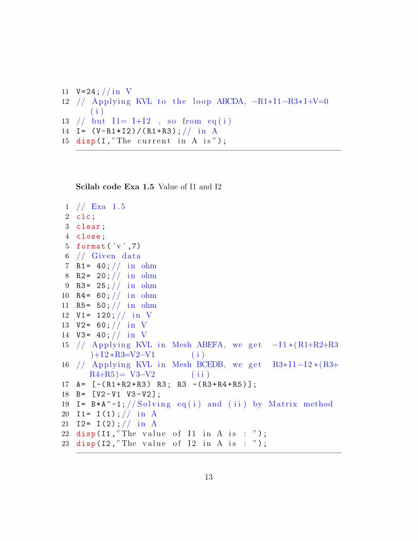
11 V=24; // i n V12 // Apply ing KVL to the l oop ABCDA, −R1∗ I1−R3∗ I+V=0

( i )13 // but I1= I+I2 , so from eq ( i )14 I= (V-R1*I2)/(R1+R3);// i n A15 disp(I,”The c u r r e n t i n A i s ”);

Scilab code Exa 1.5 Value of I1 and I2

1 // Exa 1 . 52 clc;

3 clear;

4 close;


10 R4= 60; // i n ohm11 R5= 50; // i n ohm12 V1= 120; // i n V13 V2= 60; // i n V14 V3= 40; // i n V15 // Apply ing KVL i n Mesh ABEFA, we g e t −I 1 ∗ (R1+R2+R3

)+I2 ∗R3=V2−V1 ( i )16 // Apply ing KVL i n Mesh BCEDB, we g e t R3∗ I1−I 2 ∗ (R3+

R4+R5)= V3−V2 ( i i )17 A= [-(R1+R2+R3) R3; R3 -(R3+R4+R5)];

18 B= [V2-V1 V3-V2];

19 I= B*A^-1; // S o l v i n g eq ( i ) and ( i i ) by Matr ix method20 I1= I(1);// i n A21 I2= I(2);// i n A22 disp(I1,”The v a l u e o f I 1 i n A i s : ”);23 disp(I2,”The v a l u e o f I 2 i n A i s : ”);

13

Scilab code Exa 1.6 Current through each battery and load current

1 // Exa 1 . 62 clc;

3 clear;

4 close;


10 V1= 4; // i n V11 V2= 44; // i n V12 // Apply ing KVL i n ABEFA : −R1∗ I 1 + R2∗ I 2 = V1

( i )13 // Apply ing KVL i n BCDEB: R3∗ I 1 + I2 ∗ (R2+R3)=V2 ( i i )14 A= [-R1 R3; R2 (R2+R3)]; // assumed15 B= [V1 V2]; // assumed16 I= B*A^-1; // S o l v i n g eq ( i ) and ( i i ) by Matr ix method17 I1= I(1);// i n A18 I2= I(2);// i n A19 I_L= I1+I2;// i n A20 disp(I1,”The v a l u e o f I 1 i n A i s : ”);21 disp(I2,”The v a l u e o f I 2 i n A i s : ”);22 disp(I_L ,”The v a l u e o f I L i n A i s : ”);

Scilab code Exa 1.7 Mesh analysis

1 // Exa 1 . 72 clc;

3 clear;

4 close;

14


10 R4= 1; // i n ohm11 R5= 1; // i n ohm12 V1= 1.5; // i n V13 V2= 1.1; // i n V14 // Apply ing KVL i n ABCFA : I1 ∗ (R1+R2+R3) + R3∗ I 2 =

V1 ( i )15 // Apply ing KVL i n BCDEB: R3∗ I 1 + I2 ∗ (R3+R4+R5)=V2

( i i )16 A= [(R1+R2+R3) R3; R3 (R3+R4+R5)];

17 B= [V1 V2];

18 I= B*A^-1; // S o l v i n g eq ( i ) and ( i i ) by Matr ix method19 I1= I(1);// i n A20 I2= I(2);// i n A21 disp(I1,”The v a l u e o f I 1 i n A i s : ”);22 disp(I2,”The v a l u e o f I 2 i n A i s : ”);

Scilab code Exa 1.8 Current in 6 ohm resistor

1 // Exa 1 . 82 clc;

3 clear;

4 close;


10 R4= 6; // i n ohm11 R5= 4; // i n ohm12 V1= 10; // i n V

15

13 V2= 20; // i n V14 // Apply ing KVL i n ABGHA : I1 ∗ (R1+R2) − R2∗ I 2 = V1

( i )15 // Apply ing KVL i n BCFGB : I1 ∗R5−I 2 ∗ (R3+R4+R5)+I3 ∗R4

= 0 ( i i )16 // Apply ing KVL i n CDEFC: R4∗ I2−I 3 ∗ (R2+R4)=V2

( i i i )17 A= [(R1+R2) R5 0; -R2 -(R3+R4+R5) R4; 0 R4 -(R2+R4)

];

18 B= [V1 0 V2];

19 I= B*A^-1; // S o l v i n g eq ( i ) , ( i i ) and ( i i i ) by Matr ixmethod

20 I1= I(1);// i n A21 I2= I(2);// i n A22 I3= I(3);// i n A23 I6_ohm_resistor= I2 -I3;//The c u r r e n t through 6 ohm

r e s i s t a n c e i n A24 disp(I6_ohm_resistor ,”The c u r r e n t through 6 ohm

r e s i s t a n c e i n A i s : ”)

Scilab code Exa 1.9 Current in each element

1 // Exa 1 . 92 clc;

3 clear;

4 close;


10 R4= 60; // i n ohm11 R5= 50; // i n ohm12 V= 240; // i n V13 // Apply ing KVL i n ABDA : I1 ∗−(R1+R2+R3) + R2∗ I 2+R3

16

∗ I 3 =0 ( i )14 // Apply ing KVL i n BCDB : I1 ∗R2+I2 ∗−(R2+R4+R5)+I3 ∗

R5 = 0 ( i i )15 // Apply ing KVL i n CFEADC: I1 ∗R3+ R5∗ I 2+I3 ∗−(R3+R5)=−

V ( i i i )16 A= [-(R1+R2+R3) R2 R3; R2 -(R2+R4+R5) R5; R3 R5 -(R3

+R5)];

17 B= [0 0 -V];

18 I= B*A^-1; // S o l v i n g eq ( i ) , ( i i ) and ( i i i ) by Matr ixmethod

19 I1= I(1);// i n A20 I2= I(2);// i n A21 I3= I(3);// i n A22 I30_ohm_resistor= I1;// i n A23 I60_ohm_resistor= I2;// i n A24 I50_ohm_resistor= I2-I3;// i n A25 I20_ohm_resistor= I1-I3;// i n A26 I40_ohm_resistor= I1-I2;// i n A27 disp(I30_ohm_resistor ,”The c u r r e n t through 30 ohm

r e s i s t a n c e i n A i s : ”)28 disp(I60_ohm_resistor ,”The c u r r e n t through 60 ohm




r e s i s t a n c e i n A i s : ”)3233 // Note : In the book t h e r e i s a mi s take i n eq ( i i i ) ,

the R.H. S o f eq ( i i i ) shou ld be −24 not −240.S i n c e they d i v i d e the L .H. S o f eq ( i i i ) by 10 andR.H. S not d iv ided , So the answer i n the book i swrong

17

Scilab code Exa 1.10 Value of R3 and R4

1 // Exa 1 . 1 02 clc;

3 clear;

4 close;


10 R4= 10; // i n ohm11 R5= 5; // i n ohm12 V1= 50; // i n V13 V2= 20; // i n V14 // Apply ing KCL at node A: VA∗ (R1∗R3+R3∗R2+R2∗R1)+VB

∗−R1∗R3 = V1∗R2∗R3 ( i )15 // Apply ing KCL at node B : VA∗R4∗R5+VB∗−(R2∗R4+R4∗R5

+R5∗R2) = −V2∗R2∗R4 ( i i )16 A=[(R1*R3+R2*R3+R2*R1) R4*R5; -R1*R3 -(R2*R4+R4*R5+

R5*R2)]

17 B= [V1*R2*R3 -V2*R2*R4];

18 V= B*A^-1; // S o l v i n g eq ( i ) and ( i i ) by Matr ix method19 VA= V(1);// i n V20 VB= V(2);// i n V21 I_through_R3= VA/R3;// i n A22 I_through_R4= VB/R4;// i n A23 disp(I_through_R3 ,”The c u r r e n t i n R3 i n A i s : ”)24 disp(I_through_R4 ,”The c u r r e n t i n R4 i n A i s : ”)

Scilab code Exa 1.11 Current through each resistor

1 // Exa 1 . 1 12 clc;

3 clear;

18

4 close;

5 format( ’ v ’ ,7)6 // Given data7 R1= 1; // i n ohm8 R2= 1; // i n ohm9 R3= 0.5; // i n ohm

10 R4= 2; // i n ohm11 R5= 1; // i n ohm12 V1= 15; // i n V13 V2= 20; // i n V14 // Apply ing KCL at node A: VA∗ (R1∗R2+R2∗R3+R3∗R1)+VB


+R5∗R3) = V2∗R3∗R4 ( i i )16 A=[(R1*R2+R2*R3+R3*R1) R4*R5; -R1*R2 -(R3*R4+R4*R5+

R5*R3)]

17 B= [V1*R2*R3 -V2*R3*R4];

18 V= B*A^-1; // S o l v i n g eq ( i ) and ( i i ) by Matr ix method19 VA= V(1);// i n V20 VB= V(2);// i n V21 I1= (VA -V1)/R1;// i n A22 I2= VA/R2;// i n A23 I3= (VA -VB)/R3;// i n A24 I4= VB/R4;// i n A25 I5= (VB -V2)/R5;// i n A26 disp(I1,”The v a l u e o f I 1 i n A i s : ”)27 disp(I2,”The v a l u e o f I 2 i n A i s : ”)28 disp(I3,”The v a l u e o f I 3 i n A i s : ”)29 disp(I4,”The v a l u e o f I 4 i n A i s : ”)30 disp(I5,”The v a l u e o f I 5 i n A i s : ”)


1 // Exa 1 . 1 22 clc;

19

3 clear;

4 close;

5 format( ’ v ’ ,7)6 // Given data7 V1 = 12; // i n V8 V2 = 10; // i n V9 VB = 0; // i n V

10 R1 = 2; // i n ohm11 R2 = 1; // i n ohm12 R3 = 10; // i n ohm13 // Using KCL at node A :14 VA= (V1*R2*R3+V2*R3*R1)/(R1*R2+R2*R3+R3*R1);// i n V15 I1 = (V1-VA)/R1;// i n A16 I2 = (V2-VA)/R2;// i n A17 I3 = (VA-VB)/R3;// i n A18 disp(I1,”The v a l u e o f I 1 i n A i s : ”)19 disp(I2,”The v a l u e o f I 2 i n A i s : ”)20 disp(I3,”The v a l u e o f I 3 i n A i s : ”)

Scilab code Exa 1.13 Voltage at node 1 and 2

1 // Exa 1 . 1 32 clc;

3 clear;

4 close;


10 R4= 1; // i n ohm11 I1= 1; // i n A12 I5= 2; // i n A13 // Using KCL at node 1 : V1∗ (R2+R3)−V2∗R2= I1 ∗R2∗R3

( i )

20

14 // Using KCL at node 2 : V1∗R4−V2∗ (R3+R4)= −I 5 ∗ (R3∗R4) ( i i )

15 A= [(R2+R3) R4; -R2 -(R3+R4)];

16 B= [I1*R2*R3 -I5*R3*R4];

17 V= B*A^-1; // S o l v i n g eq ( i ) and ( i i ) by Matr ix method18 V1= V(1);// i n V19 V2= V(2);// i n V20 disp(V1,”The v o l t a g e at node 1 i n v o l t s i s : ”)21 disp(V2,”The v o l t a g e at node 2 i n v o l t s i s : ”)

Scilab code Exa 1.14 Current I1 and I2

1 // Exa 1 . 1 42 clc;

3 clear;

4 close;


10 V1= 10; // i n V11 V2= 6; // i n V12 V3= 2; // i n V13 // Apply ing KVL i n ABEFA : I1 ∗ (R1+R2) − R2∗ I 2=V1−V2

( i )14 // Apply ing KVL i n BCDEB : −I 1 ∗R2+I2 ∗ (R2+R3)=V2−V3

( i i )15 A= [(R1+R2) -R2; -R2 (R2+R3)];

16 B= [(V1-V2) (V2 -V3)];

17 I= B*A^-1; // S o l v i n g eq ( i ) , and ( i i ) by Matr ixmethod

18 I1= I(1);// i n A19 I2= I(2);// i n A20 disp(I1,”The v a l u e o f I 1 i n A i s : ”)

21

21 disp(I2,”The v a l u e o f I 2 i n A i s : ”)


1 // Exa 1 . 1 52 clc;

3 clear;

4 close;


10 R4= 3; // i n ohm11 R5= 5; // i n ohm12 V1= 10; // i n V13 V2= 6; // i n V14 V3= 2; // i n V15 // Apply ing KVL i n ABEFA : I1 ∗ (R1+R2+R3) − R2∗ I 2 =

V1−V2 ( i )16 // Apply ing KVL i n BCDEB : I1∗−R2+I2 ∗ (R2+R4+R5) =V2−

V3 ( i i )17 A= [(R1+R2+R3) -R2; -R2 (R2+R4+R5)];

18 B= [(V1-V2) (V2 -V3)];

19 I= B*A^-1; // S o l v i n g eq ( i ) and ( i i ) by Matr ix method20 I1= I(1);// i n A21 I2= I(2);// i n A22 disp(I1,”The v a l u e o f I 1 i n A i s : ”)23 disp(I2,”The v a l u e o f I 2 i n A i s : ”)

Scilab code Exa 1.16 Current in resistor R1

1 // Exa 1 . 1 6

22

2 clc;

3 clear;

4 close;


10 R4= 5; // i n ohm11 V2= 10; // i n V12 I= 1; // i n A13 V1= R4*I;// i n V14 // Apply ing KVL i n ABEFA : I1 ∗ (R1+R2+R3) + R1∗ I 2 =

V1 ( i )15 // Apply ing KVL i n BCDEB : I1 ∗R1+I2 ∗ (R1+R4) =V2

( i i )16 A= [(R1+R2+R3) R1; R1 (R1+R4)];

17 B= [V1 V2];

18 I= B*A^-1; // S o l v i n g eq ( i ) and ( i i ) by Matr ix method19 I1= I(1);// i n A20 I2= I(2);// i n A21 I10_ohm= I1+I2;// i n A22 disp(I10_ohm ,”The c u r r e n t through 10 ohm r e s i s t o r i n

A i s : ”)


1 // Exa 1 . 1 72 clc;

3 clear;

4 close;

5 format( ’ v ’ ,7)6 // Given data7 R1= 4; // i n ohm8 R2= 5; // i n ohm

23

9 R3= 10; // i n ohm10 R4= 6; // i n ohm11 R5= 4; // i n ohm12 V1= 15; // i n V13 V2= 30; // i n V14 // Apply ing KCL at node A: VA∗ (R1∗R2+R2∗R3+R3∗R1)+VB


+R5∗R3) = −V2∗R3∗R4 ( i i )16 A=[(R1*R2+R2*R3+R3*R1) R4*R5; -R1*R2 -(R3*R4+R4*R5+

R5*R3)]

17 B= [V1*R1*R3 -V2*R3*R4];

18 V= B*A^-1; // S o l v i n g eq ( i ) and ( i i i ) by Matr ixmethod

19 VA= V(1);// i n V20 VB= V(2);// i n V21 I10_ohm= abs((VA-VB)/R3);// i n A22 disp(I10_ohm ,”The c u r r e n t through 10 ohm r e s i s t o r

from r i g h t to l e f t i n A i s : ”)


1 // Exa 1 . 1 92 clc;

3 clear;

4 close;


10 R4= 20; // i n ohm11 R5= 20; // i n ohm12 V= 10; // i n V13 I1= 1; // i n A

24

14 I7=0.5; // i n A15 // Apply ing KCL at node A: VA∗ (R1+R2)+VB∗−R1 = I1 ∗R1

∗R2

( i )16 // Apply ing KCL at node B : VA∗R3∗R4+VB∗−(R2∗R3+R3∗R4

+R4∗R2)+VC∗R2∗R3 = V∗R2∗R4 ( i i )17 // Apply ing KCL at node C: −VB∗R5+VC∗ (R4+R5)=I7 ∗R4∗R5

( i i i )18 A=[(R1+R2) R3*R4 0; -R1 -(R2*R3+R3*R4+R4*R2) -R5;0

R2*R3 (R4+R5)]

19 B= [I1*R1*R2 V*R2*R4 I7*R4*R5];

20 Value= B*A^-1; // S o l v i n g eq ( i ) , ( i i ) and ( i i i ) byMatr ix method

21 VA= Value (1);// i n V22 VB= Value (2);// i n V23 VC= Value (3)

24 I2= VA/R1;// i n A25 I3= (VA -VB)/R2;// i n A26 I4= (VB+V)/R3;// i n A27 I5= (VC -VB)/R4;// i n A28 I6= VC/R5;// i n A29 disp(I1,”The v a l u e o f I 1 i n A i s : ”);30 disp(I2,”The v a l u e o f I 2 i n A i s : ”);31 disp(I3,”The v a l u e o f I 3 i n A i s : ”);32 disp(I4,”The v a l u e o f I 4 i n A i s : ”);33 disp(I5,”The v a l u e o f I 5 i n A i s : ”);34 disp(I6,”The v a l u e o f I 6 i n A i s : ”);35 disp(I7,”The v a l u e o f I 7 i n A i s : ”);


1 // Exa 1 . 2 0

25

2 clc;

3 clear;

4 close;

5 format( ’ v ’ ,7)6 // Given data7 R1 = 3; // i n ohm8 R2 = 8; // i n ohm9 R3 = 4; // i n ohm

10 R4 = 12; // i n ohm11 R5 = 14; // i n ohm12 V1 = 10; // i n V13 V2 = 3; // i n V14 V3 = 6; // i n V15 // Apply ing KCL at node A: VA∗ (R1∗R2+R2∗R3+R3∗R1)+VB

∗−R1∗R2 = V1∗R2∗R3+V2∗R1∗R2 ( i )16 // Apply ing KCL at node B : VA∗R4∗R5+VB∗−(R3∗R4+R4∗R5

+R5∗R3) = V2∗R4∗R5−V3∗R3∗R4 ( i i )17 A=[(R1*R2+R2*R3+R3*R1) R4*R5; -R1*R2 -(R3*R4+R4*R5+

R5*R3)]

18 B= [(V1*R2*R3+V2*R1*R2) (V2*R4*R5-V3*R3*R4)];

19 V= B*A^-1; // S o l v i n g eq ( i ) and ( i i ) by Matr ix method20 VA= V(1);// i n V21 VB= V(2);// i n V22 I8_ohm= VA/R2;//The c u r r e n t through 8 ohm r e s i s t a n c e

i n A23 disp(I8_ohm ,”The c u r r e n t through 8 ohm r e s i s t a n c e i n

A i s : ”)

Scilab code Exa 1.21 Current drawn from the source

1 // Exa 1 . 2 12 clc;

3 clear;

4 close;

5 format( ’ v ’ ,6)

26

6 // Given data7 V= 100; // i n V8 R12 = 3; // i n ohm9 R31 = 2; // i n ohm

10 R23 = 4; // i n ohm11 R4= 6; // i n ohm12 R5=2; // i n ohm13 R6= 5; // i n ohm14 R1 = (R12*R31)/(R12+R23+R31);// i n ohm15 R2 = (R31*R23)/(R12+R23+R31);// i n ohm16 R3 = (R23*R12)/(R12+R23+R31);// i n ohm17 R_S= R6+R1;// i n ohm18 R_P1= R2+R4;// i n ohm19 R_P2= R3+R5;// i n ohm20 R_P= R_P1*R_P2/(R_P1+R_P2);// i n ohm21 R= R_P+R_S;// i n ohm22 I= V/R;// i n A23 disp(I,”The c u r r e n t drawn from the s o u r c e i n A i s :

”)

Scilab code Exa 1.22 Current in all branch

1 // Exa 1 . 2 22 clc;

3 clear;

4 close;


10 V= 100; // i n V11 I2= 10; // i n A12 // Apply ing KVL i n ABEFA : −R1∗ I1−R2∗ ( I 1+I2 )+V= 013 I1= (V-R2*I2)/(R1+R2);// i n A

27

14 I10_ohm= I1;// c u r r e n t through 10 ohm r e s i s t a n c e i n A15 I5_ohm= I1+I2;// c u r r e n t through 5 ohm r e s i s t a n c e i n

A16 I20_ohm= I2;// c u r r e n t through 20 ohm r e s i s t a n c e i n A17 disp(” Part ( i ) : Us ing by KVL”)18 disp(I10_ohm ,”The c u r r e n t through 10 ohm r e s i s t a n c e

i n A i s : ”)19 disp(I5_ohm ,”The c u r r e n t through 5 ohm r e s i s t a n c e i n

A i s : ”)20 disp(I20_ohm ,”The c u r r e n t through 20 ohm r e s i s t a n c e

i n A i s : ”)21 // Apply ing KCL at node A :22 VA= (V*R2+I2*R1*R2)/(R1+R2);// i n V23 I10_ohm= (VA -V)/R1;// i n A24 I5_ohm= VA/R2;// i n A25 I20_ohm= I2;// i n A26 disp(” Part ( i i ) : Us ing by KVL”)27 disp(I10_ohm ,”The c u r r e n t through 10 ohm r e s i s t a n c e

i n A i s : ”)28 disp(I5_ohm ,”The c u r r e n t through 5 ohm r e s i s t a n c e i n

A i s : ”)29 disp(I20_ohm ,”The c u r r e n t through 20 ohm r e s i s t a n c e

i n A i s : ”)

Scilab code Exa 1.23 Current and voltage across 2 ohm resistor

1 // Exa 1 . 2 32 clc;

3 clear;

4 close;


28

10 R4= 2; // i n ohm11 V1= 10; // i n V12 V2= 20; // i n V13 I= 5; // i n A14 // Apply ing KCL at node A: VA∗ (R1+R2)+VB∗−R1 =I ∗R1∗

R2+V1∗R1(

i )15 // Apply ing KCL at node B : VA∗R3∗R4+VB∗−(R2∗R3+R4∗R3

+R4∗R2) =V1∗R3∗R4+V2∗R2∗R3 ( i i )16 A=[(R1+R2) R3*R4; -R1 -(R3*R2+R4*R3+R4*R2)]

17 B= [(I*R1*R2+V1*R1) (V1*R3*R4+V2*R2*R3)];

18 V= B*A^-1; // S o l v i n g eq ( i ) and ( i i ) by Matr ix method19 VA= V(1);// i n V20 VB= V(2);// i n V21 I4= (VB+V2)/R4;// i n A22 V4= R4*I4;// i n V23 disp(I4,”The c u r r e n t through 2 ohm r e s i s t o r i n A i s

: ”)24 disp(V4,”The v o l t a g e a c r o s s 2 ohm r e s i s t o r i n V i s :

”)

Scilab code Exa 1.24 Voltage across 6 ohm resistor

1 // Exa 1 . 2 42 clc;

3 clear;

4 close;


10 R4= 6; // i n ohm11 V2= 12; // i n V

29

12 V3= 30; // i n V13 // Apply ing KVL i n ABEFA : I1 ∗ (R1+R2) − R2∗ I 2=V3−V2

( i )14 // Apply ing KVL i n BCDEB : −I 1 ∗R2+I2 ∗ (R1+R2+R3)=V2

( i i )15 A= [(R1+R2) -R2; -R2 (R1+R2+R3)];

16 B= [(V3-V2) (V2)];

17 I= B*A^-1; // S o l v i n g eq ( i ) , and ( i i ) by Matr ixmethod

18 I1= I(1);// i n A19 I2= I(2);// i n A20 V1= I2*R1;// v o l t a g e a c r o s s 6 ohm r e s i s t o r i n V21 disp(V1,”The v o l t a g e a c r o s s 6 ohm r e s i s t o r i n V i s :

”)

Scilab code Exa 1.25 Resistance between point B and C

1 // Exa 1 . 2 52 clc;

3 clear;

4 close;


10 R4 = 4; // i n ohm11 R5 = 4; // i n ohm12 R6 = 6; // i n ohm13 R12= R1*R2/(R1+R2);// i n ohm14 R34= R3*R4/(R3+R4);// i n ohm15 R56= R5*R6/(R5+R6);// i n ohm16 // R e s i s t a n c e between the p o i n t B and C17 R_BC= (R12+R34)*R56 /((R12+R34)+R56);// i n ohm18 disp(R_BC ,”The r e s i s t a n c e between the p o i n t B and C

30

i n ohm i s : ”)

Scilab code Exa 1.26 Voltage across R1 and R2

1 // Exa 1 . 2 62 clc;

3 clear;

4 close;


10 V1= 100; // i n V11 I2= 0.5; // i n A12 V2= I2*R4;// i n V13 // Apply ing KVL : −R1∗ I1−V2+V1−R1∗ I 2=014 I1= (V1 -V2)/(R1+R2);// i n A15 V_R1= I1*R1;// v o l t a g e a c r o s s R1 r e s i s t o r i n V16 V_R2= I1*R2;// v o l t a g e a c r o s s R2 r e s i s t o r i n V17 disp(V_R1 ,”The v o l t a g e a c r o s s R1 r e s i s t o r i n V i s :

”)18 disp(V_R2 ,”The v o l t a g e a c r o s s R2 r e s i s t o r i n V i s :

”)


1 // Exa 1 . 2 72 clc;

3 clear;

4 close;

5 format( ’ v ’ ,5)6 // Given data

31

7 R1 = 8; // i n ohm8 R2 = 4; // i n ohm9 R3 = 4; // i n ohm

10 R4 = 4; // i n ohm11 R5 = 8; // i n ohm12 R6 = 8; // i n ohm13 I=10; // i n A14 V= 20; // i n V15 // Apply ing KVL i n ABEFA : I1 ∗ (R1+R2+R3)+I2 ∗ (R3)= I ∗

R2−V ( i )16 // Apply ing KVL i n BCDEB : I1 ∗R3−I 2 ∗ (R3+R4+R5)= R4∗ I

+V ( i i )17 A= [(R1+R2+R3) R3; R3 -(R3+R4+R5)];

18 B= [I*R2 -V R4*I+V];

19 I= B*A^-1; // // S o l v i n g e q u a t i o n s by matr ixm u l t i p l i c a t i o n

20 I1= I(1);// i n A21 I2= I(2);// i n A22 disp(I1,”The v a l u e o f I 1 i n A i s : ”);23 disp(I2,”The v a l u e o f I 2 i n A i s : ”);

32

Chapter 2

Network Theorems

Scilab code Exa 2.1 Current through load resistance

1 // Exa 2 . 12 clc;

3 clear;

4 close;


10 V = 24; // i n V11 R_T =R1+R1*R2/(R1+R2);// i n ohm12 I_T = V/R_T;// i n A13 I1 = (R1/(R1+R2))*I_T;// i n A14 V = 12; // i n V15 I_T = V/R_T;// i n A16 I2 = (R1/(R1+R2))*I_T;// i n A17 I = I1+I2;// i n A18 disp(I,”The c u r r e n t i n A i s ”);

33

Scilab code Exa 2.2 Value of current across 12 ohm

1 // Exa 2 . 22 clc;

3 clear;

4 close;

5 format( ’ v ’ ,5)6 // Given data7 R1 = 5; // i n ohm8 Vth= 10; // i n ohm9 R2 = 7; // i n ohm

10 R3=10; // i n ohm11 R_L = 12; // i n ohm12 V = 20; // i n ohm13 Vth = (Vth*V)/(R1+R3);// i n V14 Rth = R2 + ((Vth*R1)/(Vth+R1));// i n ohm15 // The c u r r e n t through 12 ohm r e s i s t o r16 I = Vth/(Rth+R_L);// i n A17 disp(I,”The c u r r e n t through 12 ohm r e s i s t o r i n A i s ”

);

Scilab code Exa 2.3 Value of current across 12 ohm

1 // Exa 2 . 32 clc;

3 clear;

4 close;


10 R_L = 12; // i n ohm11 V = 30; // i n V12 Vth = (R3*V)/(R3+R1);// i n V

34

13 Rth = R2 + ((R3*R1)/(R3+R1)) ;// i n ohm14 I_N = Vth/Rth;// i n A15 //The c u r r e n t through 12 ohm r e s i s t o r16 I = (I_N*Rth)/(Rth+R_L);// i n ohm17 disp(I,”The c u r r e n t through 12 ohm r e s i s t o r i n A i s ”

);

Scilab code Exa 2.4 Load resistor

1 // Exa 2 . 42 clc;

3 clear;

4 close;


10 V = 20; // i n V11 Vth = R2*V/(R1+R2);// i n V12 Rth = R3 + ((R2*R1)/(R2+R1));// i n ohm13 R_L = Rth;// i n ohm14 disp(R_L ,”The v a l u e o f l o ad r e s i s t a n c e i n ohm i s ”);15 Pmax = (Vth^2) /(4* R_L);// i n W16 disp(Pmax ,”The magnitude o f maximum power i n W i s ”);

Scilab code Exa 2.5 Current across 4 ohm resistor

1 // Exa 2 . 52 clc;

3 clear;

4 close;

5 format( ’ v ’ ,5)

35

6 // Given data7 V1 = 12; // i n V8 V2 = 10; // i n V9 R1 = 6; // i n ohm

10 R2 = 7; // i n ohm11 R3 = 4; // i n ohm12 R_T = R1 + ( (R2*R3)/(R2+R3) );// i n ohm13 I_T = V1/R_T;// i n A14 I1 = (R2/(R2+R3))*I_T;// i n A15 R_T = R2 + ( (R1*R3)/(R1+R3) );// i n ohm16 I_T = V2/R_T;// i n A17 I2 = (R1*I_T)/(R1+R3);// i n A18 // c u r r e n t a c r o s s 4 ohm r e s i s t o r19 I = I1+I2;// i n A20 disp(I,”The c u r r e n t a c r o s s 4 ohm r e s i s t o r i n A i s ”);

Scilab code Exa 2.6 Current in branch AB

1 // Exa 2 . 62 clc;

3 clear;

4 close;


10 R4= 2; // i n ohm11 V1 = 4.2; // i n V12 V2 = 3.5; // i n V13 R_T =R1+R3+R2*R4/(R2+R4);// i n ohm14 I_T = V1/R_T;// i n A15 I1 = (R1/(R1+R2))*I_T;// i n A16 R = R1+R3;// i n ohm17 R_desh = (R*R2)/(R+R2);// i n ohm

36

18 R_T = R_desh+R1;// i n ohm19 I_T = V2/R_T;// i n A20 I2 = (R2/(R2+R))*I_T;// i n A21 // c u r r e n t i n the branch AB22 I = I2 -I1;// i n A23 disp(I,”The c u r r e n t i n the branch AB o f the c i r c u i t

i n A i s ”);

Scilab code Exa 2.7 Current through 8 ohm resistor

1 // Exa 2 . 72 clc;

3 clear;

4 close;


10 Ig = 2; // i n A11 V = 20; // i n V12 R_T = R1+R3;// i n ohm13 I1 = V/R_T;// i n A14 I2 = (R1/(R1+R3))*Ig;// i n A15 // c u r r e n t through i n 8 ohm r e s i s t o r16 I = I1 -I2;// i n A17 disp(I,”The c u r r e n t through i n 8 ohm r e s i s t o r i n A

i s ”);

Scilab code Exa 2.8 Current across 16 ohm resistor

1 // Exa 2 . 82 clc;

37

3 clear;

4 close;

5 format( ’ v ’ ,7)6 // Given data7 R1 = 4; // i n ohm8 R2 = 24; // i n ohm9 R_L = 16; // i n ohm

10 V1 = 20; // i n V11 V2 = 30; // i n V12 // V1−R1∗ I−R2∗ I−V2 = 0 ;13 I= (V1-V2)/(R1+R2)

14 // V1−R1∗ I−Vth = 0 ;15 Vth = V1 -R1*I;// i n V16 Rth = (R1*R2)/(R1+R2);// i n ohm17 // c u r r e n t through 16 ohm r e s i s t o r18 I_L = Vth/(Rth+R_L);// i n A19 disp(I_L ,”The c u r r e n t through 16 ohm r e s i s t o r i n A

i s ”);

Scilab code Exa 2.9 Current through 6 ohm resistor

1 // Exa 2 . 92 clc;

3 clear;

4 close;


10 R_L = 6; // i n ohm11 V1 = 6; // i n V12 V2 = 15; // i n V13 // V1 − R1∗ I − R3∗ I −V2 = 014 I= (V1-V2)/(R1+R3);

38

15 // Vth − R3∗ I −V2 = 0 ;16 Vth =V2+R3*I;// i n V17 Rth = ((R1*R3)/(R1+R3)) + R2;// i n ohm18 // c u r r e n t through 6 ohm r e s i s t a n c e19 I_L = Vth/(Rth+R_L);// i n A20 disp(I_L ,”The c u r r e n t through 6 ohm r e s i s t a n c e i n A

i s ”);


1 // Exa 2 . 1 02 clc;

3 clear;

4 close;


10 R_L = 10; // i n ohm11 V1= 20; // i n V12 V2= 12; // i n V13 // V1−R3∗ I − R2∗ I = 0 ;14 I = V1/(R2+R3);// i n A15 // Vth + V2 − R3∗ I = 0 ;16 Vth = R3*I - V2;// i n V17 Rth = ((R2*R3)/(R2+R3)) + R1;// i n ohm18 // c u r r e n t through 10 ohm r e s i s t a n c e19 I_L = abs(Vth)/(Rth+R_L);// i n A20 disp(I_L ,”The c u r r e n t through 10 ohm r e s i s t a n c e i n A

i s ”);


39

1 // Exa 2 . 1 12 clc;

3 clear;

4 close;


10 R_L = 5; // i n ohm11 I = 6; // i n A12 V = 15; // i n V13 // V−R1∗ I1−R3∗ ( I 1+I ) = 0 ;14 I1 = (V-R3*I)/(R1+R3);// i n A15 I = I1 + I;// i n A16 Vth = R3*I;// i n V17 Rth = ((R1*R3)/(R1+R3)) + R2;// i n ohm18 // c u r r e n t i n 5 ohm r e s i s t a n c e19 I_L = Vth/(Rth+R_L);// i n A20 disp(I_L ,”The c u r r e n t i n 5 ohm r e s i s t a n c e i n A i s ”);

Scilab code Exa 2.12 Thevenins equivalent of the netword

1 // Exa 2 . 1 22 clc;

3 clear;

4 close;

5 format( ’ v ’ ,5)6 // Given data7 R1 = 8; // i n ohm8 R2 = 32; // i n ohm9 V = 60; // i n V

10 I1= 5; // i n A11 I2= 3; // i n A12 // Vth−R1∗ I1 −( I 1+I2 ) ∗R2−V=0

40

13 Vth= R1*I1+(I1+I2)*R2+V

14 Rth = R1+R2;// i n ohm15 disp(Vth ,”The v a l u e o f Vth i n v o l t s i s : ”)16 disp(Rth ,”The v a l u e o f Rth i n ohm i s : ”);


1 clc;

2 clear;

3 close;

4 format( ’ v ’ ,5)5 // Given data6 R1 = 6; // i n ohm7 R2 = 4; // i n ohm8 R3 = 3; // i n ohm9 R_L = 6; // i n ohm

10 V1 = 6; // i n V11 V2= 15; // i n V12 // V1 − R1∗ I − R3∗ I −V2 = 0 ;13 I= (V1-V2)/(R1+R3)

14 Vth = V2 + (R3*I);// i n V15 Rth = ((R1*R3)/(R1+R3)) + R2;// i n ohm16 I_N = Vth/Rth;// i n A17 // c u r r e n t through 6 ohm r e s i s t o r18 I = (I_N*Rth)/(Rth+R_L);// i n A19 disp(I,”The c u r r e n t through 6 ohm r e s i s t o r i n A i s ”)

;


1 // Exa 2 . 1 42 clc;

3 clear;

41

4 close;


10 V1 = 20; // i n V11 V2 = 12; // i n V12 // V1−R2∗ I−R1∗ I = 0 ;13 I = V1/(R1+R2);// i n A14 // Vth + V2 − R2∗ I = 0 ;15 Vth = (R2*I) - V2;// i n V16 Rth = ((R1*R2)/(R1+R2)) + R3;// i n ohm17 I_N = Vth/Rth;// i n A18 R_L = 10; // i n ohm19 // c u r r e n t through 10 ohm r e s i s t a c e20 I = (abs(I_N)*Rth)/(Rth+R_L);// i n A21 disp(I,”The c u r r e n t through 10 ohm r e s i s t a c e i n A i s

”);


1 // Exa 2 . 1 52 clc;

3 clear;

4 close;

5 format( ’ v ’ ,6)6 // Given data7 V = 15; // i n V8 R1 = 4; // i n ohm9 R2 = 3; // i n ohm

10 R3 = 2; // i n ohm11 R_L = 5; // i n ohm12 Ig = 6; // i n A13 // V − R1∗ I 1 − R3∗ ( I 1+Ig ) = 0 ;

42

14 I1 = (V-R3*Ig)/(R1+R3);// i n A15 I = I1 + Ig;// i n A16 Vth = R3*I;// i n V17 Rth = ((R1*R3)/(R1+R3)) + R2;// i n ohm18 I_N = Vth/Rth;// i n A19 // c u r r e n t through 5 ohm r e s i s t o r20 I = (I_N*Rth)/(Rth+R_L);// i n A21 disp(I,”The c u r r e n t through 5 ohm r e s i s t o r i n A i s ”)

;

Scilab code Exa 2.16 Value of R

1 // Exa 2 . 1 62 clc;

3 clear;

4 close;


10 R3 = 3; // i n ohm11 R4 = 2; // i n ohm12 Rth=(R1*R2/(R1+R2)+R3)*R4/((R1*R2/(R1+R2)+R3)+R4)

13 R_L = Rth;// i n ohm14 disp(R_L ,”The v a l u e o f R i n ohm i s ”);

Scilab code Exa 2.17 Load Resistance and power delivered to load

1 // Exa 2 . 1 72 clc;

3 clear;

4 close;

43


10 V = 20; // i n V11 // V − R1∗ I 1 − R2∗ I 1 = 0 ;12 I1 = V/(R1+R2);// i n A13 Vth = R1*I1;// i n V14 Rth =R1*R2/(R1+R2)+R3

15 R_L = Rth;// i n ohm16 disp(R_L ,”The v a l u e o f l o ad r e s i s t a n c e i n ohm i s ”);17 Pmax = (Vth^2) /(4* Rth);// i n W18 disp(Pmax ,”The power d e l i v e r e d to the l oad i n W i s ”)

;


1 // Exa 2 . 1 82 clc;

3 clear;

4 close;


10 V1 = 120; // i n V11 V2 = 60; // i n V12 R = (R3*R2)/(R3+R2);// i n ohm13 R_T = R+R1;// i n ohm14 I_T = V1/R_T;// i n A15 I1 = (R2/(R2+R3)) * I_T;// i n A16 R_T = 2 + R2;// i n ohm17 I_T = V2/R_T;// i n A

44

18 I2 = (R1/(R1+R3)) * I_T;// i n A19 // c u r r e n t through 6 ohm r e s i s t o r20 I = I1 -I2;// i n A21 disp(I,”The c u r r e n t through 6 ohm r e s i s t o r i n A i s ”)

;


1 // Exa 2 . 1 92 clc;

3 clear;

4 close;


10 V1 = 90; // i n V11 V2 = 60; // i n V12 R_T = (R2*R3)/(R2+R3)+R1;// i n ohm13 I_T = V1/R_T;// i n A14 I1 = (R2/(R2+R3)) * I_T;// i n A15 R = (R1*R3)/(R1+R3);// i n ohm16 R_T = R2+R;// i n ohm17 I_T = V2/R_T;// i n A18 I2 = (R1/(R1+R3))*I_T;// i n A19 Ra = (R1*R2)/(R1+R2);// i n ohm asumed20 I_T = 2; // i n A21 I3 = (Ra/(Ra+R3))*I_T;// i n A22 // c u r r e n t i n 8 ohm r e s i s t o r23 I = I1+I2+I3;// i n A24 disp(I,”The c u r r e n t i n 8 ohm r e s i s t o r i n A i s ”);

45

Scilab code Exa 2.20 Thevenins equivalent circuit

1 // Exa 2 . 2 02 clc;

3 clear;

4 close;


10 V1 = 60; // i n v11 V2 = 30; // i n V12 //−R1∗ i 1 − R3∗ i 1 − V2+V1 = 0 ;13 i1 = (V2-V1)/(R1+R3);// i n A14 V_acrossR3 = R3*i1;// i n V15 Vth = V_acrossR3+V1;// i n V16 V_AB =Vth;// i n V17 disp(V_AB ,”The Theven ins v o l t a g e i n V i s ”);18 R = (R1*R3)/(R1+R3);// i n ohm19 Rth = R2+R;// i n ohm20 disp(Rth ,”The Theven ins r e s i s t a n c e i n ohm i s ”);


1 // Exa 2 . 2 12 clc;

3 clear;

4 close;


10 R_L = 5; // i n ohm

46

11 V = 15; // i n V12 I2 = 6; // i n A13 // −R1∗ I 1 − R3∗ I 1 + R3∗ I 2 + V = 0 ;14 I1 = (V+R3*I2)/(R1+R3);// i n A15 Vth = I2/R3;// i n V16 V_CD = Vth;// i n V17 Rth = (R1*R3)/(R1+R3)+R2;// i n ohm18 I = Vth/(Rth+R_L);// i n A19 disp(I,”The c u r r e n t f l o w i n g through 5 ohm r e s i s t o r

i n A i s ”);

Scilab code Exa 2.22 Norton equivalent circuit

1 // Exa 2 . 2 22 clc;

3 clear;

4 close;


10 R4 = 2; // i n ohm11 V = 30; // i n V12 I1=4; // i n A13 V1= I1*R3;// i n V14 // R1∗ I −R2∗ I+V = 0 ;15 I = V/(R1+R2);// i n A16 V_acrossR2= R2*I;// i n V17 V_AB = V_acrossR2 -V1;// i n V18 Vth = abs(V_AB);// i n V19 Rth = (R1*R2)/(R1+R2)+R3+R4;// i n ohm20 disp(Rth ,”The v a l u e o f Rth i n ohm i s ”);21 I_N = Vth/Rth;// i n A22 disp(I_N ,”The v a l u e o f I N i n A i s ”);

47

Scilab code Exa 2.23 Vth and Rth

1 // Exa 2 . 2 32 clc;

3 clear;

4 close;


10 R4 = 4; // i n ohm11 V = 16; // i n v12 I1= 8; // i n A13 V1= I1*R2;// i n V14 I2= 16; // i n A15 V2= I2*R3;// i n V16 // Apply ing KVL : R2∗ I+V1+R3∗ I−V2+V+R1∗ I17 I= (V2-V1 -V)/(R1+R2+R3);// i n A18 Vth= V2-R3*I;// i n V19 Rth= (R1+R2)*R3/((R1+R2)+R3)+R4;// i n ohm20 disp(Vth ,”The v a l u e o f Vth i n v o l t s i s : ”)21 disp(Rth ,”The v a l u e o f Rth i n ohm i s : ”)

Scilab code Exa 2.24 Load resistance

1 // Exa 2 . 2 42 clc;

3 clear;

4 close;

5 format( ’ v ’ ,5)

48

6 // Given data7 R1 = 3; // i n ohm8 R2 = 2; // i n ohm9 R3 = 1; // i n ohm

10 R4 = 8; // i n ohm11 R5 = 2; // i n ohm12 V = 10; // i n V13 R = ((R1+R2)*R5)/((R1+R2)+R5);// i n ohm14 Rth = R + R3;// i n ohm15 R_L = Rth;// i n ohm16 disp(R_L ,”The v a l u e o f l o ad r e s i s t a n c e i n ohm i s ”);

Scilab code Exa 2.25 Load resistance and maximum power

1 // Exa 2 . 2 52 clc;

3 clear;

4 close;


10 R3 = 10; // i n ohm11 R4 = 10; // i n ohm12 I2 = 20; // i n A.13 // Apply ing KVL i n GEFHG : −R1∗ I1−R2∗ I1−R2∗ I 2 + V =

0 ;14 I1= (V-R2*I2)/(R1+R2);// i n A15 V_AB= R3*I2+V-R1*I1;// i n V16 Vth = V_AB;// i n V17 Rth = (R1*R2)/(R1+R2)+R3+R4;// i n ohm18 R_L = Rth;// i n ohm19 disp(R_L ,”The v a l u e o f R L i n ohm i s ”);20 Pmax = (Vth^2) /(4* R_L);//maximum power i n W

49

21 disp(Pmax ,”The v a l u e o f maximum power i n W i s ”);


1 // Exa 2 . 2 62 clc;

3 clear;

4 close;


10 V1 = 6; // i n v11 V2 = 12; // i n V12 // −R2∗ Ix −R1∗ Ix−V1+V2= 0 ;13 Ix = (V2-V1)/(R1+R2);// i n A14 Vth = V1+R1*Ix;// i n V15 Rth = (R1*R2)/(R1+R2);// i n ohm16 I_N = Vth/Rth;// i n A17 I = (I_N*Rth)/(Rth+R_L);// i n A18 disp(I,”The c u r r e n t i n A i s ”);1920 // Note : At l a s t , t h e r e i s c a l c u l a t i o n e r r o r to f i n d

the v a l u e o f I , so the answer i n the book i swrong .


1 // Exa 2 . 2 72 clc;

3 clear;

4 close;

50


10 V = 27; // i n V11 I=3; // i n A12 // −I 1+I2= I ( i )13 // Apply ing KVL: I1 ∗R1+I2 ∗R2=V ( i i )14 A= [-1 R1; 1 R2];

15 B= [I V]

16 I= B*A^-1; // S o l v i n g eq ( i ) and ( 2 ) by Matr ix method17 I1= I(1);// i n A18 I2= I(2);// i n A19 Vth= R2*I2;// i n V20 Rth= R1*R2/(R1+R2);// i n ohm21 // c u r r e n t i n 4 ohm r e s i s t o r22 I= Vth/(Rth+R_L);// i n A23 disp(I,”The c u r r e n t i n 4 ohm r e s i s t o r i n A i s : ”)


1 // Exa 2 . 2 82 clc;

3 clear;

4 close;


10 V1 = 90; // i n V11 V2 = 60; // i n V12 R_T = R1 + ((R2*R3)/(R2+R3));// i n ohm13 I_T = V1/R_T;// i n A

51

14 I1 = I_T;// i n A15 R_T = R2 + ((R1*R3)/(R1+R3));// i n ohm16 I_T = V2/R_T;// i n A17 I2 = (R3/(R3+R1))*I_T;// i n A18 R_T = R1 + ((R2*R3)/(R2+R3));// i n ohm19 I_T = 2; // i n A ( g i v e n )20 R = (R2*R3)/(R2+R3);// i n ohm21 I3 = (R/(R1+R))*I_T;// i n A22 // c u r r e n t i n 20 ohm r e s i s t o r23 I20 = I1 -I2-I3;// i n A24 disp(I20 ,”The c u r r e n t i n 20 ohm r e s i s t o r i n A i s ”);

Scilab code Exa 2.29 Current in resistor R2

1 // Exa 2 . 2 92 clc;

3 clear;

4 close;


10 R4 = 30; // i n ohm11 E1 = 120; // i n V12 E2 = 60; // i n V13 R_T = ((R2*R3)/(R2+R3)) + R4+R1;// i n ohm14 I_T = E1/R_T;// i n A15 I1 = (R3/(R2+R3))*I_T;// i n A16 R_T = ( ((R1+R4)*R2)/((R1+R4)+R2) ) + R3;// i n ohm17 I_T = E2/R_T;// i n A18 I2 = ((R1+R4)/(R1+R4+R2))*I_T;// i n A19 // c u r r e n t through R2 r e s i s t o r20 I= I1+I2;// i n A21 disp(I,”The c u r r e n t through R2 r e s i s t o r i n A i s ”);

52

Scilab code Exa 2.30 Current in all resistor

1 // Exa 2 . 3 02 clc;

3 clear;

4 close;


10 Ig = 3; // i n A11 V = 15; // i n V12 I1 = R1/(R1+R2)*Ig;// i n A13 I2 = -I1;// i n A14 I3 = 0; // i n A15 R_T = ((R1+R2)*R3)/((R1+R2)+R3);// i n ohm16 I_T = V/R_T;// i n A17 I_2= R3/(R1+R2+R3)*I_T;// i n A18 I_1 = I_2;// i n A19 // Tota l c u r r e n t through upper 4 r e s i s t o r20 tot_cur_up_4ohm= I1+I2;// i n A21 // Tota l c u r r e n t through l owe r 4 r e s i s t o r22 tot_cur_low_4ohm= I_1+I_2;// i n A23 // Tota l c u r r e n t through 8 r e s i s t o r24 tot_cur_8ohm= I3+I_T;// i n A25 disp(tot_cur_up_4ohm ,” Tota l c u r r e n t through upper 4

r e s i s t o r i n A i s : ”)26 disp(tot_cur_low_4ohm ,” Tota l c u r r e n t through l owe r 4

r e s i s t o r i n A i s : ”)27 disp(tot_cur_8ohm ,” Tota l c u r r e n t through 8

r e s i s t o r i n A i s : ”)

53

Scilab code Exa 2.31 Current in all resistor

1 // Exa 2 . 3 12 clc;

3 clear;

4 close;


10 V = 10; // i n V11 Ig = 2; // i n A12 I2 = (R1/R3)*Ig;// i n A13 I1 = I2;// i n A14 I3 = 0; // i n A15 R_T = ((R1+R2)*R3)/((R1+R2)+R3);// i n ohm16 I_T = V/R_T;// i n A17 I_2 = (R3/((R1+R2)+R3))*I_T;// i n A18 I_1 = I_2;// i n A19 I_3 = I_1;// i n A20 // Tota l c u r r e n t through upper i n 5 r e s i s t o r21 tot_cur_up_5ohm = I1-I2;// i n A22 // Tota l c u r r e n t through l owe r i n 5 r e s i s t o r23 tot_cur_low_5ohm = I_1+I_2;// i n A24 // Tota l c u r r e n t through 10 r e s i s t o r25 tot_cur_10ohm = I3+I_3;// i n A26 disp(tot_cur_up_5ohm ,”The t o t a l c u r r e n t through

upper i n 5 r e s i s t o r i n A i s ”);27 disp(tot_cur_low_5ohm ,”The t o t a l c u r r e n t through

l owe r i n 5 r e s i s t o r i n A i s ”);28 disp(tot_cur_10ohm ,”The t o t a l c u r r e n t through i n 10

r e s i s t o r i n A i s ”);

54

Chapter 3

AC fundamental

Scilab code Exa 3.2 Time period

1 // Exa 3 . 22 clc;

3 clear;

4 close;

5 format( ’ v ’ ,7)6 // Given data7 Im = 141.4; // i n A8 t = 3; // i n ms9 t = t * 10^-3; // i n s e c

10 disp(Im,”The maximum v a l u e o f c u r r e n t i n A i s ”);11 omega = 314; // i n rad / s e c12 // omega = 2∗%pi∗ f ;13 f = round(omega /(2* %pi));// i n Hz14 disp(f,”The f r e q u e n c y i n Hz i s ”);15 T = 1/f;// i n s e c16 disp(T,”The t ime p e r i o d i n s e c i s ”);17 i = 141.4 * sin(omega*t);// i n A18 disp(i,”The i n s t a n t a n e o u s v a l u e i n A i s ”);

55


1 // Exa 3 . 32 clc;

3 clear;

4 close;

5 format( ’ v ’ ,8)6 // Given data7 f = 60; // i n Hz8 Im = 120; // i n A9 t = 1/360; // i n s e c

10 omega = 2*%pi*f;// i n rad / s e c11 i = Im*sin(omega*t);// i n A12 disp(i,”The v a l u e o f c u r r e n t a f t e r 1/360 s e c i n A i s

”);13 i = 96; // i n A14 // i = Im∗ s i n d ( omega∗ t ) ;15 t = (asin(i/Im))/omega;// i n s e c16 disp(t,”The t ime taken to r each 96 A f o r the f i r s t

t ime i n s e c i s ”);

Scilab code Exa 3.4 Average and RMS value

1 // Exa 3 . 42 clc;

3 clear;

4 close;

5 format( ’ v ’ ,6)6 // Given data7 i1 = 0; // i n A8 i2 = 10; // i n A9 i3 = 20; // i n A

10 i4 = 30; // i n A11 i5 = 20; // i n A12 i6 = 10; // i n A

56

13 n = 6; // u n i t l e s s14 Iav = (i1+i2+i3+i4+i5+i6)/n;// i n A15 disp(Iav ,”The ave rage v a l u e i n A i s ”);16 Irms = sqrt(( (i1^2) + (i2^2) + (i3^2) + (i4^2) + (

i5^2) + (i6^2) )/n);// i n A17 disp(Irms ,”The RMS v a l u e i n A i s ”);18 k_f = Irms/Iav;// u n i t l e s s19 disp(k_f ,”The form f a c t o r i s ”);20 Im = 30; // i n A21 k_p = Im/Irms;// u n i t l e s s22 disp(k_p ,”The peak f a c t o r i s ”);

Scilab code Exa 3.5 Phase difference

1 // Exa 3 . 52 clc;

3 clear;

4 close;

5 format( ’ v ’ ,6)6 // Given data7 theta1 = 60; // i n d e g r e e8 theta2 = -45; // i n d e g r e e9 // phase d i f f e r e n c e

10 phi = theta1 -theta2;// i n d e g r e e11 disp(phi ,”The phase d i f f e r e n c e i n d e g r e e i s ”);

Scilab code Exa 3.6 Instantaneous values of sum and difference of voltage

1 // Exa 3 . 62 clc;

3 clear;

4 close;

5 format( ’ v ’ ,7)

57

6 // Givven data7 V1= 60* expm(%i*0* %pi /180);// i n V8 V2= 40* expm(%i*-%pi/3);// i n V9 add_V= V1+V2;// i n V

10 diff_V= V1-V2;// i n V11 disp(”The sum o f V1 and V2 i s : ”)12 disp(string(abs(add_V))+” s i n ( t h e t a ”+string(atand(

imag(add_V),real(add_V)))+” ) V”)13 disp(”The d i f f e r e n c e o f V1 and V2 i s : ”)14 disp(string(abs(diff_V))+” s i n ( t h e t a+”+string(atand

(imag(diff_V),real(diff_V)))+” ) V”)

Scilab code Exa 3.7 Average value effective value and form factor

1 // Exa 3 . 72 clc;

3 clear;

4 close;

5 format( ’ v ’ ,6)6 // Givven data7 Vo= 1; // i n V ( assumed )8 Vav= integrate( ’Vo∗ s i n ( t h e t a ) ’ , ’ t h e t a ’ ,0,%pi)/(2* %pi

);

9 Vrms= sqrt(integrate( ’Voˆ2∗(1− co s (2∗ t h e t a ) ) /2 ’ , ’t h e t a ’ ,0,%pi))*sqrt (1/(2* %pi));

10 kf= Vrms/Vav;

11 disp(”The ave rage v a l u e o f output v o l t a g e i n v o l t si s : ”+string(Vav)+”∗Vo or Vo/%pi”)

12 disp(”The R.M. S v a l u e o f output v o l t a g e i n v o l t s i s: ”+string(Vrms)+”∗Vo or Vo/2 ”)

13 disp(kf,”The form f a c t o r i s : ”)

Scilab code Exa 3.8 Average and RMS value

58

1 // Exa 3 . 82 clc;

3 clear;

4 close;

5 format( ’ v ’ ,5)6 // Given data7 T = 0.3; // i n s e c8 V = 20; // i n V9 Vav = 1/T*V*integrate( ’ 1 ’ , ’ t ’ ,0,0.1)

10 disp(Vav ,”The ave rage v a l u e o f v o l t a g e i n V i s ”);11 Vrms =sqrt (1/T*V^2* integrate( ’ 1 ’ , ’ t ’ ,0,0.1))12 disp(Vrms ,”The R.M. S v a l u e o f v o l t a g e i n V i s ”);

Scilab code Exa 3.9 Rectangular form of voltage

1 // Exa 3 . 92 clc;

3 clear;

4 close;

5 format( ’ v ’ ,6)6 // Given data7 Vm = 100; // i n V8 phi = %pi/6; // i n d e g r e e9 Vrms = Vm/(sqrt (2));// i n V

10 // Rec tangu l a r form o f the v o l t a g e11 RectForm= Vrms*expm(%i*phi)

12 disp(RectForm ,” Rec tangu l a r form o f the v o l t a g e i n Vi s : ”)

13 disp(” Po la r form o f the v o l t a g e : ”)14 disp(” Magnitude o f v o l t a g e i n V i s : ”+string(abs(

RectForm))+” V”)15 disp(” Angle i s : ”+string(atand(imag(RectForm),real(

RectForm)))+” ”)

59

Scilab code Exa 3.10 Phaser diagram

1 // Exa 3 . 1 02 clc;

3 clear;

4 close;

5 format( ’ v ’ ,7)6 // Given data7 V1= 100/ sqrt (2)*expm(%i*0* %pi /180);// i n V8 V2= 200/ sqrt (2)*expm(%i*60* %pi /180);// i n V9 V3= 50/ sqrt (2)*expm(%i*-90*%pi /180);// i n V

10 V4= 150/ sqrt (2)*expm(%i*-45*%pi /180);// i n V11 // The R.M. S . v a l u e o f the r e s u l t a n t12 V_R= real(V1)+real(V2)+real(V3)+real(V4);// i n V13 disp(V_R ,”The R.M. S . v a l u e o f the r e s u l t a n t i n v o l t s

i s : ”)


1 // Exa 3 . 1 12 clc;

3 clear;

4 close;

5 format( ’ v ’ ,7)6 // Given data7 Im = 15; // i n A8 f = 60; // i n Hz9 omega = 2*%pi * f;// i n rad / s e c

10 t = 1/200; // i n s e c11 i = Im*sin(omega*t);// i n A12 disp(i,”The v a l u e o f c u r r e n t a f t e r 1/200 s e c i n A i s

”);

60

13 i = 10; // i n A14 // i = Im∗ s i n d ( omega∗ t ) ;15 t = (asin(i/Im))/omega;// i n s e c16 t = t * 10^3; // i n ms17 disp(t,”The t ime to r each 10 A i n ms i s ”);18 Iav = Im *0.637; // i n A19 disp(Iav ,”The ave rage v a l u e i n A i s ”);

Scilab code Exa 3.12 Maximum current frequency and RMS value andform factor

1 // Exa 3 . 1 22 clc;

3 clear;

4 close;

5 format( ’ v ’ ,5)6 // Given data7 Im = 42.42; // i n A8 omega = 628; // i n rad / s e c9 t = 1/6.977; // i n s e c assumed

10 i = Im*sind(omega*t);// i n A11 disp(i,”The maximum v a l u e o f c u r r e n t i n A i s ”);12 // omega = 2∗%pi∗ f ;13 f = omega /(2* %pi);// i n Hz14 disp(f,”The f r e q u e n c y i n Hz i s ”);15 Irms = Im/(sqrt (2));// i n A16 disp(Irms ,”The rms v a l u e i n A i s ”);17 Iav = (2*Im)/%pi;// i n A18 disp(Iav ,”The ave rage v a l u e i n A i s ”);19 k_f = Irms/Iav;

20 disp(k_f ,”The form f a c t o r i s ”);

Scilab code Exa 3.13 Power factor and RMS value of current

61

1 // Exa 3 . 1 32 clc;

3 clear;

4 close;

5 format( ’ v ’ ,6)6 // Given data7 phi = %pi/6;

8 // Power f a c t o r9 powerfactor = cos(phi);// i n l a g

10 disp(powerfactor ,”The power f a c t o r i s ”);11 Im = 22; // i n A12 // The R.M. S v a l u e o f c u r r e n t13 Irms = Im/sqrt (2);// i n A14 disp(Irms ,”The R.M. S v a l u e o f c u r r e n t i n A i s ”);15 omega = 314; // i n rad / s e c16 // omega = 2∗%pi∗ f ;17 f = omega /(2* %pi);// i n Hz18 disp(f,”The f r e q u e n c y i n Hz i s ”);

Scilab code Exa 3.14 RMS value average value and form factor

1 // Exa 3 . 1 42 clc;

3 clear;

4 close;

5 format( ’ v ’ ,6)6 // Given data7 Im= 100; // i n A8 Irms= sqrt(Im ^2/2* integrate( ’1−co s (2∗ t h e t a ) ’ , ’ t h e t a ’

,0,%pi)/%pi);// i n A9 disp(Irms ,”The R.M. S v a l u e o f c u r r e n t i n A i s : ”)

10 Iav= Im*integrate( ’ s i n ( t h e t a ) ’ , ’ t h e t a ’ ,0,%pi)/%pi;//i n A

11 disp(Iav ,”The ave rage v a l u e o f c u r r e n t i n A i s : ”)12 // The form f a c t o r

62

13 kf= Irms/Iav;


Scilab code Exa 3.15 Form factor

1 // Exa 3 . 1 52 clc;

3 clear;

4 close;

5 format( ’ v ’ ,6)6 // Given data7 A= 2*10; // a r ea under curve f o r a c y c l e8 B= 2; // base o f h a l f c y c l e9 Vav= 1/2*A/B;// i n V

10 // For l i n e AB11 y1= 0;

12 y2= 10;

13 x1= 0;

14 x2= 1;

15 m_for_AB= (y2-y1)/(x2 -x1);

16 // For l i n e BC17 y1= 10;

18 y2= 0;

19 x1= 1;

20 x2= 2;

21 m_for_BC= (y2-y1)/(x2 -x1);

22 Vrms= sqrt(( integrate( ’ ( m for AB ∗ t ) ˆ2 ’ , ’ t ’ ,0,1)+integrate( ’ ( m for BC ∗ t +20) ˆ2 ’ , ’ t ’ ,1,2))/2);// i nV

23 kf= Vrms/Vav;


63

Chapter 4

Three Phase AC Circuits

Scilab code Exa 4.1 Current and power consumed

1 // Exa 4 . 12 clc;

3 clear;

4 close;

5 format( ’ v ’ ,6)6 // Given data7 R = 10; // inohm8 V = 230; // i n V9 f = 50; // i n Hz

10 I = V/R;// i n A11 disp(I,”The c u r r r e n t i n A i s ”);12 P =V*I;// i n W13 disp(P,”The power consumed i n W i s ”);14 Vm = sqrt (2)*V;// i n V15 Im =sqrt (2)*I;// i n A16 omega = 2*%pi*f;// i n rad / s e c17 // Equat ion f o r v o l t a g e : V = Vm∗ s i n d ( omega∗ t )18 // Equat ion f o r c u r r e n t : i = Im∗ s i n d ( omega∗ t )19 disp(” Vo l tage e q u a t i o n : v = ”+string(Vm)+” s i n ( ”+

string(round(omega))+” t ) ”)20 disp(” Current e q u a t i o n : i = ”+string(Im)+” s i n ( ”+

64

string(round(omega))+” t ) ”)

Scilab code Exa 4.2 Instantaneous power and average power

1 // Exa 4 . 22 clc;

3 clear;

4 close;

5 format( ’ v ’ ,6)6 // Given data7 R = 100; // i n ohm8 i= ’ 3∗ co s ( omega∗ t ) ’ ;// i n A9 A= R*3^2; // assumed

10 disp(” I n s t a n t a n e o u s power taken by r e s i s t o r i n watt si s : ”)

11 disp(string(A/2)+” (1+ co s (2∗ omega∗ t ) ) ”)12 P= R*3^2/2*(1+ cos(%pi/2));// i n watt s13 disp(P,”The ave rage power i n watt s i s : ”)

Scilab code Exa 4.3 Inductive reactance

1 // Exa 4 . 32 clc;

3 clear;

4 close;

5 format( ’ v ’ ,6)6 // Given data7 I = 10; // i n A8 V = 230; // i n V9 f = 50; // i n Hz

10 X_L = V/I;// i n ohm11 disp(X_L ,” I n d u c t i v e r e a c t a n c e i n ohm i s ”);12 // X L = 2∗%pi∗ f ∗L ;

65

13 L = X_L /(2* %pi*f);// i n H14 disp(L,” Induc tance o f the c o i l i n H i s ”);15 Vrms = V;// i n V16 Irms = I;// i n A17 Vm = Vrms*sqrt (2);// i n V18 Im = Irms*sqrt (2);// i n A19 omega = 2*%pi*f;// i n rad / s e c20 // Equat ion f o r v o l t a g e : V = Vm∗ s i n d ( omega∗ t )21 // Equat ion f o r c u r r e n t : i = Im∗ s i n d ( omega∗ t )22 disp(” Vo l tage e q u a t i o n : v = ”+string(Vm)+” s i n ( ”+


string(round(omega))+” t − %pi /2) ”)

Scilab code Exa 4.4 Capacitive reactance

1 // Exa 4 . 42 clc;

3 clear;

4 close;

5 format( ’ v ’ ,6)6 // GIven data7 C = 318; // i n F8 C = C * 10^-6; // i n F9 V = 230; // i n V

10 f = 50; // i n Hz11 X_C = 1/(2* %pi*f*C);// i n ohm12 disp(X_C ,”The c a p a c i t i v e r e a c t a n c e i n ohm i s ”);13 I = V/X_C;// i n A14 disp(I,”The R.M. S v a l u e o f c u r r e n t i n A i s ”);15 Vrms = V;// i n V16 Irms = I;// i n A17 Vm = Vrms*sqrt (2);// i n V18 Im = Irms*sqrt (2);// i n A19 omega = 2*%pi*f;// i n rad / s e c

66

20 // V = Vm∗ s i n d ( omega∗ t ) ;21 // i = Im∗ s i n d ( ( omega∗ t ) +(%pi /2) ) ;22 // Equat ion f o r v o l t a g e : V = Vm∗ s i n d ( omega∗ t )23 // Equat ion f o r c u r r e n t : i = Im∗ s i n d ( omega∗ t )24 disp(” Vo l tage e q u a t i o n : v = ”+string(Vm)+” s i n ( ”+


string(round(omega))+” t + %pi /2) ”)

Scilab code Exa 4.5 Circuit current

1 // Exa 4 . 52 clc;

3 clear;

4 close;

5 format( ’ v ’ ,6)6 // Given data7 R = 7; // i n ohm8 L = 31.8; // i n mH9 L = L * 10^-3; // i n H

10 V = 230; // i n V11 f = 50; // i n Hz12 X_L = 2*%pi*f*L;// i n ohm13 Z = sqrt( (R^2)+(X_L ^2) );// i n ohm14 I = V/Z;// i n A15 disp(I,”The c i r c u i t c u r r e n t i n A i s ”);16 // tand ( ph i ) = X L/R;17 phi = atand(X_L/R);// i n d e g r e e l a g18 disp(phi ,”The phase a n g l e i n d e g r e e i s ”);19 // Power f a c t o r20 powerfactor = cosd(phi);// i n l a g21 disp(powerfactor ,”The power f a c t o r i s ”);22 P = V*I*cosd(phi);// i n W23 disp(P,”The power consumed i n W i s ”);

67

Scilab code Exa 4.6 Value of R and L

1 // Exa 4 . 62 clc;

3 clear;

4 close;

5 format( ’ v ’ ,6)6 // Given data7 P = 400; // i n W8 f = 50; // i n Hz9 V = 120; // i n V

10 phi= acosd (0.8);// i n11 // P =V∗ I ∗ co s ( ph i ) ;12 I = P/(V*cosd(phi));// i n A13 Z= V/I;// i n ohm14 Z= Z*expm(%i*phi*%pi /180);// ohm15 R= real(Z);// i n ohm16 XL= imag(Z);// i n ohm17 // Formula XL= 2∗%pi∗ f ∗L18 L= XL/(2* %pi*f);// i n H19 disp(R,”The v a l u e o f R i n i s : ”)20 disp(L,”The v a l u e o f L i n H i s : ”)

Scilab code Exa 4.7 Active and reactive component of current

1 // Exa 4 . 72 clc;

3 clear;

4 close;

5 format( ’ v ’ ,6)6 // Given data7 R = 17.32; // i n ohm

68

8 L = 31.8; // i n mH9 L = L * 10^-3; // i n H

10 V = 200; // i n V11 f = 50; // i n Hz12 X_L = 2*%pi*f*L;// i n ohm13 Z = sqrt( (R^2) + (X_L ^2) );// i n ohm14 I = V/Z;// i n A15 phi =acosd( R/Z);// i n16 ActiveCom= I*cosd(phi);// i n A17 ReactiveCom= I*sind(phi);// i n A18 disp(ActiveCom ,”The a c t i v e component o f c u r r e n t i n A

i s : ”)19 disp(ReactiveCom ,”The r e a c t i v e component o f c u r r e n t

i n A i s : ”)20 P= V*I*cosd(phi);// i n W21 disp(P,”The a c t i v e power i n W i s : ”)22 Q= V*I*sind(phi);// i n VAR23 disp(Q,”The r e a c t i v e power i n VAR i s : ”)2425 // Note : There i s c a l c u l a t i o n e r r o r to e v a l u a t e the

v a l u e o f P , so the answer i n the book i s wrong .

Scilab code Exa 4.8 Voltage across each component and circuit

1 // Exa 4 . 82 clc;

3 clear;

4 close;

5 format( ’ v ’ ,7)6 // Given data7 R = 20; // i n ohm8 C = 200; // i n F9 C=C*10^-6

10 f =50; // i n Hz11 // I = 1 0 . 8 s i n (314∗ t )

69

12 Im = 10.8; // i n A13 I = Im/sqrt (2);// i n A14 V_R = I*R;// i n V15 disp(V_R ,”The v o l t a g e a c r o s s 20 r e s i s t o r i n V i s :

”)16 //Vc = I ∗X C and X C = 1/ omega∗C;17 omega = 2*%pi*f;// i n rad / s e c18 Vc = I * 1/( omega*C);// i n V19 disp(Vc,”The v o l t a g e a c r o s s 200 F c a p a c i t o r i n V

i s ”);20 V = sqrt( (V_R^2) + (Vc^2) );// i n V21 disp(V,”The v o l t a g e a c r o s s the c i r c u i t i n V i s ”);

Scilab code Exa 4.9 Resistance and inductance

1 // Exa 4 . 92 clc;

3 clear;

4 close;

5 format( ’ v ’ ,6)6 // Given data7 f= 60; // i n Hz8 disp(” Part ( a ) ”)9 Z= 12+30* %i;

10 R= real(Z);// i n ohm11 XL= imag(Z);// i n ohm12 // Formula XL= 2∗%pi∗ f ∗L13 L= XL/(2* %pi*f);// i n H14 L= L*10^3; // i n mH15 disp(R,”The v a l u e o f r e s i s t a n c e i n i s : ”)16 disp(L,”The v a l u e o f i n d u c t a n c e i n mH i s : ”)17 L= L*10^ -3; // i n H18 disp(” Part ( b ) ”)19 Z= 0-60*%i;

20 R= real(Z);// i n ohm

70

21 XC= (abs(imag(Z)));// i n ohm22 // Formula XC= 1/(2∗%pi∗ f ∗C)23 C= 1/(2* %pi*XC*f);// i n H24 C= C*10^6; // i n F25 disp(R,”The v a l u e o f r e s i s t a n c e i n i s : ”)26 disp(C,”The v a l u e o f i n d u c t a n c e i n F i s : ”)27 C= C*10^ -6; // i n F28 disp(” Part ( c ) ”)29 Z= 20* expm (60*%i*%pi /180)

30 R= real(Z);// i n ohm31 XL= imag(Z);// i n ohm32 // Formula XL= 2∗%pi∗ f ∗L33 L= XL/(2* %pi*f);// i n H34 L= L*10^3; // i n mH35 disp(R,”The v a l u e o f r e s i s t a n c e i n i s : ”)36 disp(L,”The v a l u e o f i n d u c t a n c e i n mH i s : ”)

Scilab code Exa 4.10 Power factor supply voltage and active and reactivepower

1 // Exa 4 . 1 02 clc;

3 clear;

4 close;

5 format( ’ v ’ ,7)6 // Given data7 R = 120; // i n ohm8 XC = 250; // i n ohm9 I = 0.9; // i n A

10 Z= R-%i*XC;// i n ohm11 phi= atand(imag(Z),real(Z))

12 V=I*Z;// i n V13 VR = I*R;// i n V14 VC= I*XC;// i n V15 P= abs(V)*I*cosd(phi);// i n W

71

16 Q= abs(V)*I*sind(phi);// i n VAR17 disp(cosd(phi),”The power f a c t o r i s : ”)18 disp(” Supply v o l t a g e : ”)19 disp(” Magnitude i s : ”+string(abs(V))+” V and a n g l e

i s : ”+string(atand(imag(V),real(V)))+” ”)20 disp(VR,”The v o l t a g e a c r o s s r e s i s t a n c e i n V i s : ”)21 disp(VC,”The v o l t a g e a c r o s s c a p a c i t a n c e i n V i s : ”)22 disp(P,”The a c t i v e power i n W i s : ”)23 disp(Q,”The r e a c t i v e power i n VAR i s : ”)

Scilab code Exa 4.11 Impedance current power factor and power consumed

1 // Exa 4 . 1 12 clc;

3 clear;

4 close;

5 format( ’ v ’ ,7)6 // Given data7 V = 230; // i n V8 f = 50; // i n Hz9 L = 0.06; // i n H

10 R = 2.5; // i n ohm11 C = 6.8; // i n F12 C = C * 10^-6; // i n F13 X_L = 2*%pi*f*L;// i n ohm14 X_C = 1/(2* %pi*f*C);// i n ohm15 Z = sqrt( (R^2) + ((X_L -X_C)^2) );// i n ohm16 disp(Z,”The impedance i n ohm i s ”);17 I = V/Z;// i n A18 disp(I,”The c u r r e n t i n A i s ”);19 // tan ( ph i ) = ( X L−X C) /R;20 phi = atand( (X_L -X_C)/R );// i n l e a d21 disp(”The phase a n g l e between c u r r e n t and v o l t a g e i s

: ”+string(abs(phi))+” l e a d ”);22 phi = acosd(R/Z);

72

23 disp(”The power f a c t o r i s : ”+string(cosd(phi))+”l e a d ”);

24 P = V*I*cosd(phi);// i n W25 disp(P,”The power consumed i n W i s ”);

Scilab code Exa 4.12 The resonant frequency

1 // Exa 4 . 1 22 clc;

3 clear;

4 close;

5 format( ’ v ’ ,9)6 // GIven data7 R = 100; // i n ohm8 L = 100; // i n H9 L = L * 10^-6; // i n H

10 C = 100; // i n pF11 C = C * 10^ -12; // i n F12 V = 10; // i n V13 // The r e s o n a n t f r e q u e n c y14 f_r = 1/(2* %pi*sqrt(L*C));// i n Hz15 disp(f_r ,”The r e s o n a n t f r e q u e n c y i n Hz i s ”);16 // c u r r e n t at r e s o n a n c e17 Ir = V/R;// i n A18 disp(Ir,”The c u r r e n t at r e s o n a n c e i n A i s ”);19 X_L = 2*%pi*f_r*L;// i n ohm20 // v o l t a g e a c r o s s L at r e s o n a n c e21 V_L = Ir*X_L;// i n V22 disp(V_L ,”The v o l t a g e a c r o s s L at r e s o n a n c e i n V i s ”

);

23 X_C = X_L;// i n ohm24 // v o l t a g e a c r o s s C at r e s o n a n c e25 V_C = Ir*X_C;// i n V26 disp(V_C ,”The v o l t a g e a c r o s s C at r e s o n a n c e i n V i s ”

);

73

27 Q= 1/R*sqrt(L/C);

28 disp(Q,”The Q− f a c t o r i s : ”)

Scilab code Exa 4.13 Frequency at resonance

1 // Exa 4 . 1 32 clc;

3 clear;

4 close;

5 format( ’ v ’ ,7)6 // Given data7 R = 10; // i n ohm8 L = 0.2; // i n H9 C = 40; // i n F

10 C = C * 10^-6; // i n F11 V = 100; // i n V12 f_r = 1/(2* %pi*sqrt(L*C));// i n Hz13 disp(f_r ,”The f r e q u e n c y at r e s o n a c e i n Hz i s ”);14 Im = V/R;// i n A15 disp(Im,”The c u r r e n t i n A i s ”);16 Pm = (Im^2)*R;// i n W17 disp(Pm,”The power i n W i s ”);18 // v o l t a g e a c r o s s R19 V_R = Im*R;// i n V20 disp(V_R ,”The v o l t a g e a c r o s s R i n V i s ”);21 X_L = 2*%pi*f_r*L;// i n ohm22 // v o l t a g e a c r o s s L23 V_L = Im*X_L;// i n V24 disp(V_L ,”The v o l t a g e a c r o s s L i n V i s ”);25 X_C = 1/(2* %pi*f_r*C);// i n ohm26 // v o l t a g e a c r o s s C27 V_C = Im*X_C;// i n V28 disp(V_C ,”The v o l t a g e a c r o s s C i n V i s ”);29 omega = 2*%pi*f_r;// i n rad / s e c30 Q = (omega*L)/R;

74

31 disp(Q,”The q u a l i t y f a c t o r i s ”);32 del_F = R/(4* %pi*L);

33 f1 = f_r -del_F;// i n Hz34 f2 = f_r+del_F;// i n Hz35 disp(”The h a l f power f r e q u e n c i e s a r e : ”+string(f1)+

” Hz and ”+string(f2)+” Hz”);36 BW = f2-f1;// i n Hz37 disp(BW,”The bandwidth i n Hz i s : ”)

Scilab code Exa 4.14 Bandwidth

1 // Exa 4 . 1 42 clc;

3 clear;

4 close;

5 format( ’ v ’ ,6)6 // Given data7 R = 10; // i n ohm8 L = 15; // i n H9 L = L * 10^-6; // i n H

10 C = 100; // i n pF11 C = C * 10^ -12; // i n F12 f_r = 1/(2* %pi*sqrt(L*C));// i n Hz13 X_L = 2*%pi*f_r*L;// i n ohm14 Q = X_L/R;// i n ohm15 BW = f_r/Q;// i n Hz16 BW = BW * 10^ -3; // i n kHz17 disp(BW,”The bandwidth i n kHz i s ”);

Scilab code Exa 4.15 Half power points

1 // Exa 4 . 1 52 clc;

75

3 clear;

4 close;

5 format( ’ v ’ ,6)6 // Given data7 R = 1000; // i n ohm8 L = 100; // i n mH9 L = L * 10^-3; // i n H

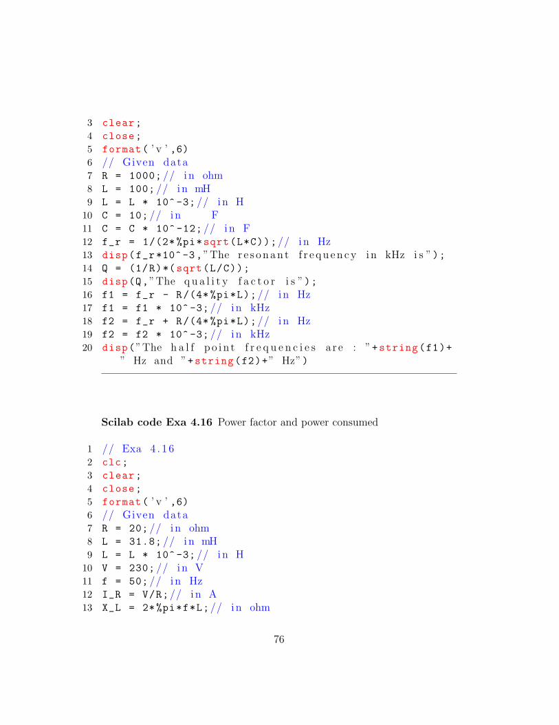
10 C = 10; // i n F11 C = C * 10^ -12; // i n F12 f_r = 1/(2* %pi*sqrt(L*C));// i n Hz13 disp(f_r*10^-3,”The r e s o n a n t f r e q u e n c y i n kHz i s ”);14 Q = (1/R)*(sqrt(L/C));

15 disp(Q,”The q u a l i t y f a c t o r i s ”);16 f1 = f_r - R/(4* %pi*L);// i n Hz17 f1 = f1 * 10^ -3; // i n kHz18 f2 = f_r + R/(4* %pi*L);// i n Hz19 f2 = f2 * 10^ -3; // i n kHz20 disp(”The h a l f p o i n t f r e q u e n c i e s a r e : ”+string(f1)+

” Hz and ”+string(f2)+” Hz”)

Scilab code Exa 4.16 Power factor and power consumed

1 // Exa 4 . 1 62 clc;

3 clear;

4 close;

5 format( ’ v ’ ,6)6 // Given data7 R = 20; // i n ohm8 L = 31.8; // i n mH9 L = L * 10^-3; // i n H

10 V = 230; // i n V11 f = 50; // i n Hz12 I_R = V/R;// i n A13 X_L = 2*%pi*f*L;// i n ohm

76

14 I_L = V/X_L;// i n A15 I = sqrt( (I_R^2) + (I_L^2) );// i n A16 disp(I,”The l i n e c u r r e n t i n A i s ”);17 phi= acosd( I_R/I);

18 disp(”The power f a c t o r i s : ”+string(cosd(phi))+”l a g ”);

19 P = V*I*cosd(phi);// i n W20 disp(P,”The power consumed i n W i s ”);


1 // Exa 4 . 1 72 clc;

3 clear;

4 close;

5 format( ’ v ’ ,6)6 // Given data7 C = 50; // i n F8 C = C * 10^-6; // i n F9 R = 20; // i n ohm

10 L = 0.05; // i n H11 V = 200; // i n V12 f = 50; // i n Hz13 X_C = 1/(2* %pi*f*C);// i n ohm14 Z1 = X_C;// i n ohm15 I1 = V/X_C;// i n A16 X_L = 2*%pi*f*L;// i n ohm17 Z2 = sqrt( (R^2) + (X_L^2) );// i n ohm18 I2 = V/Z2;// i n A19 // tan ( ph i2 ) = X L/R;20 phi2 = atand(X_L/R);// i n d e g r e e21 phi1 = 90; // i n d e g r e e22 I_cos_phi = I1*cosd(phi1) + I2*cosd(phi2);// i n A23 I_sin_phi = I1*sind(phi1) - I2*sind(phi2);// i n A24 phi= atand(I_sin_phi/I_cos_phi);// i n

77

25 I= sqrt(I_cos_phi ^2+ I_sin_phi ^2);// i n A26 P= V*I*cosd(phi);// i n W27 disp(I,”The l i n e c u r r e n t i n A i s : ”)28 disp(”The power f a c t o r i s : ”+string(cosd(phi))+”

l a g ”);29 disp(P,”The power consumed i n W i s : ”)

Scilab code Exa 4.18 Power factor

1 // Exa 4 . 1 82 clc;

3 clear;

4 close;

5 format( ’ v ’ ,6)6 // Given data7 V= 68+154* %i;// i n V8 I1= 10+14* %i;// i n A9 I2= 2+8*%i;// i n A

10 I= I1+I2;// i n A11 phi= atand(imag(V),real(V))-atand(imag(I),real(I));

// i n12 disp(phi ,”The phase a n g l e i n i s : ”)13 disp(”The power f a c t o r i s : ”+string(cosd(phi))+”

l a g ”)

Scilab code Exa 4.19 Supply current and power factor

1 // Exa 4 . 1 92 clc;

3 clear;

4 close;

5 format( ’ v ’ ,6)6 // Given data

78

7 R1 = 50; // i n ohm8 L = 318; // i n mH9 L = L * 10^-3; // i n H

10 R2 = 75; // i n ohm11 C = 159; // i n F12 C =C * 10^ -6; // i n F13 V = 230; // i n V14 f = 50; // i n Hz15 XL= 2*%pi*f*L;// i n ohm16 Z1= R1+XL*%i;// i n ohm17 I1= V/Z1;// i n A18 XC= 1/(2* %pi*f*C);// i n ohm19 Z2= R2 -%i*XC;// i n ohm20 I2= V/Z2;// i n A21 I= I1+I2;// i n A22 phi= atand(imag(I),real(I));// i n23 disp(” Supply c u r r e n t : ”)24 disp(” Magnitude i s : ”+string(abs(I))+” A”)25 disp(” Angle : ”+string(phi)+” ”)26 disp(”Power f a c t o r i s : ”+string(cosd(phi))+” l a g ”)

Scilab code Exa 4.20 Supply current and power factor

1 // Exa 4 . 2 02 clc;

3 clear;

4 close;

5 format( ’ v ’ ,6)6 // Given data7 V=250; // i n V8 Z1= 70.7+70.7* %i;// i n ohm9 Z2= 120+160* %i;// i n ohm

10 Z3= 120+90* %i;// i n ohm11 Y1= 1/Z1;// i n S12 Y2= 1/Z2;// i n S

79

13 Y3= 1/Z3;// i n S14 Y_T= Y1+Y2+Y3;// i n S15 phi= atand(imag(Y_T),real(Y_T));// i n16 disp(” Tota l admi t tance o f the c i r c u i t : ”)17 disp(” Magnitude i s : ”+string(abs(Y_T))+” mho”)18 disp(” Angle i s : ”+string(phi)+” ”)19 I= V*Y_T;// i n A20 disp(”The supp ly c u r r e n t : ”)21 disp(” Magnitude i s : ”+string(abs(I))+” A”)22 disp(” Angle i s : ”+string(phi)+” ”)23 disp(”Power f a c t o r i s : ”+string(cosd(phi))+” l a g

”)

Scilab code Exa 4.21 Power and power factor

1 // Exa 4 . 2 12 clc;

3 clear;

4 close;

5 format( ’ v ’ ,6)6 // Given data7 Vm = 100; // i n V8 phi1= 30; // i n9 Im = 15; // i n A

10 phi2= 60; // i n11 V= Vm/sqrt (2)*expm(phi1*%i*%pi /180);// i n V12 I= Im/sqrt (2)*expm(phi2*%i*%pi /180);// i n A13 Z= V/I;// i n ohm14 R= real(Z);// i n ohm15 XC= abs(imag(Z));// i n ohm16 phi= atand(imag(Z),real(Z));// i n17 P= abs(V)*abs(I)*cosd(phi);// i n W18 disp(”The impedance i s : ”+string(Z)+” ”)19 disp(”The r e s i s t a n c e i s : ”+string(R)+” ”)20 disp(”The r e a c t a n c e i s : ”+string(XC)+” ”)

80

21 disp(”The power i s : ”+string(P)+” W”)22 disp(”The power f a c t o r i s : ”+string(cosd(phi))+”

l e a d i n g ”)

Scilab code Exa 4.22 Value of pure indutance

1 // Exa 4 . 2 22 clc;

3 clear;

4 close;

5 format( ’ v ’ ,6)6 // Given data7 P = 100; // i n W8 V = 120; // i n V9 f= 50; // i n Hz

10 I = P/V;// i n A11 V = 200; // i n V12 V_R = 120; // i n V13 V_L = sqrt( (V^2) - (V_R ^2) );// i n V14 // V L = I ∗X L ;15 X_L = V_L/I;// i n ohm16 // X L = 2∗%pi∗ f ∗L ;17 L = X_L /(2* %pi*f);// i n H18 disp(L,”The v a l u e o f pure i n d u c t a n c e i n H i s ”);1920 // Note : There i s c a l c u l a t i o n e r r o r to f i n d the

v a l u e o f V L , So the answer i n the book i s wrongand cod ing i s c o r r e c t .


1 // Exa 4 . 2 32 clc;

81

3 clear;

4 close;

5 format( ’ v ’ ,6)6 // Given data7 V=230; // i n V8 f= 50; // i n Hz9 Z1= 10* expm (-30*%i*%pi /180);// i n ohm

10 Z2= 20* expm (60*%i*%pi /180);// i n ohm11 Z3= 40* expm (0*%i*%pi /180);// i n ohm12 Y1= 1/Z1;// i n S13 Y2= 1/Z2;// i n S14 Y3= 1/Z3;// i n S15 Y= Y1+Y2+Y3;// i n S16 phi= atand(imag(Y),real(Y));// i n17 Z=1/Y;// i n ohm18 P= V^2* abs(Y);// i n W19 disp(”The c i r c u i t admit tance i s : ”+string(abs(Y))+”

mho”);20 disp(”The c i r c u i t impedance i s : ”+string(abs(Z))+”

”);21 disp(P,”The power consumed i n W i s : ”)22 disp(”The power f a c t o r i s : ”+string(cosd(phi))+”

l e a d ”)

Scilab code Exa 4.24 Current and power absorbed by each branch

1 // Exa 4 . 2 42 clc;

3 clear;

4 close;

5 format( ’ v ’ ,8)6 // Given data7 Z1= 10+15* %i;// i n ohm8 Z2= 6-8*%i;// i n ohm9 R1= 10; // i n ohm

82

10 R2= 6; // i n ohm11 I_T= 15; // i n A12 I1= I_T*Z2/(Z1+Z2);// i n A13 I2= I_T*Z1/(Z1+Z2);// i n A14 P1= (abs(I1))^2*R1;// i n W15 P2= (abs(I2))^2*R2;// i n W16 disp(P1,”The v a l u e o f P1 i n W i s : ”)17 disp(P2,”The v a l u e o f P2 i n W i s : ”)

Scilab code Exa 4.25 Voltage across the condenser

1 // Exa 4 . 2 52 clc;

3 clear;

4 close;


10 C = C * 10^-6; // i n F11 V = 230; // i n V12 f = 50; // i n Hz13 XL = 2*%pi*f*L;// i n ohm14 XC= 1/(2* %pi*f*C);// i n ohm15 Z= R+%i*XL -%i*XC;// i n ohm16 I= V/Z;// i n A17 phi= atand(imag(I),real(I));// i n18 PowerFactor= cosd(phi);

19 VC= abs(I)*XC;// i n V20 disp(” Impedence o f the e n t i r e c i r c u i t : ”)21 disp(” Magnitude i s : ”+string(abs(Z))+” ”);22 disp(” Angle i s : ”+string(atand(imag(Z),real(Z)))+”

”)23 disp(” Current f l o w i n g through the condenso r : ”)

83

24 disp(” Magnitude i s : ”+string(abs(I))+” ”);25 disp(” Angle i s : ”+string(atand(imag(I),real(I)))+”

”)26 disp(”Power f a c t o r o f the c i r c u i t i s : ”+string(cosd

(phi))+” l a g ”)27 disp(VC,”The v o l t a g e a c r o s s the condenso r i n V i s :

”)

Scilab code Exa 4.26 Half power frequencies

1 // Exa 4 . 2 62 clc;

3 clear;

4 close;


10 C = C * 10^-6; // i n F11 f_r = 1/(2* %pi*sqrt(L*C));// i n Hz12 Q = (1/R) * (sqrt(L/C));

13 del_F = R/(4* %pi*L);

14 // The h a l f power f r e q u e n c i e s15 f1 = f_r - del_F;// i n Hz16 f2 = f_r+del_F;// i n Hz17 disp(”The h a l f power f r e q u e n c i e s a r e : ”+string(f1)+

” Hz and ”+string(f2)+” Hz”)

Scilab code Exa 4.27 Value of capacitor

1 // Exa 4 . 2 72 clc;

84

3 clear;

4 close;

5 format( ’ v ’ ,6)6 // Given data7 R = 15; // i n ohm8 X_L = 10; // i n ohm9 f_r = 50; // i n Hz

10 // X L = 2∗%pi∗ f r ∗L ;11 L = X_L /(2* %pi*f_r);// i n H12 // v a l u e o f c a p a c i t a n c e13 C = 1/( L*( ((f_r*2*%pi)^2) +((R^2)/(L^2)) ));// i n F14 C = C*10^6; // i n F15 disp(C,”The v a l u e o f c a p a c i t a n c e i n F i s ”);

Scilab code Exa 4.28 Current and power drawn

1 // Exa 4 . 2 82 clc;

3 clear;

4 close;

5 format( ’ v ’ ,6)6 // Given data7 Z1= 3+4*%i;// i n ohm8 Z2= 6+8*%i;// i n ohm9 V= 230; // i n V

10 I1= V/Z1;// i n A11 I2= V/Z2;// i n A12 I_T= I1+I2;// i n A13 phi= atand(imag(I_T),real(I_T));// i n14 P= V*abs(I_T)*cosd(phi);// i n V15 disp(”The v a l u e o f c u r r e n t : ”)16 disp(abs(I_T),”The magnitude i n A i s : ”)17 disp(phi ,”The phase a n g l e i n d e g r e e i s : ”)18 disp(P,”The power drawn from the s o u r c e i n W i s : ”)

85

Scilab code Exa 4.29 Total power supplied by source

1 // Exa 4 . 2 92 clc;

3 clear;

4 close;

5 format( ’ v ’ ,6)6 // Given data7 Z1= 1.6+%i *7.2; // i n ohm8 Z2= 4+%i*3; // i n ohm9 Z3= 6-%i*8; // i n ohm

10 V= 100; // i n V11 Y2= 1/Z2;// i n mho12 disp(Y2,”The admit tance i n mho i s : ”)13 Y3= 1/Z3;// i n mho14 disp(Y3,”The admit tance i n mho i s : ”)15 ZT= Z1+1/(Y2+Y3);

16 phi= atand(imag(ZT),real(ZT));

17 disp(” Tota l c i r c u i t impedance : ”)18 disp(” Magnitude : ”+string(abs(ZT))+” ”)19 disp(” Angle : ”+string(phi)+” ”);20 IT= V/ZT;// i n A21 PT= V*abs(IT)*cosd(phi);// i n W22 disp(PT,”The t o t a l power s u p p l i e d i n W i s : ”)

Scilab code Exa 4.30 Q factor of the circuit

1 // Exa 4 . 3 02 clc;

3 clear;

4 close;

5 format( ’ v ’ ,6)

86

6 // Given data7 R = 4; // i n ohm8 L = 0.5; // i n H9 V = 100; // i n V

10 f = 50; // i n Hz11 X_L = 2*%pi*f*L;// i n ohm12 X_C = X_L;// i n ohm13 // X C = 1/(2∗%pi∗ f ∗C) ;14 C = 1/(X_C*2* %pi*f);// i n F15 C = C * 10^6; // i n F16 disp(C,”The v a l u e o f c a p a c i t a n c e i n F i s ”);17 I = V/R;// i n A]18 V_C = I*X_C;// i n V19 disp(V_C ,”The v o l t a g e a c r o s s the c a p a c i t a n c e i n V”);20 omega = 2*%pi*f;// i n rad / s e c21 Q = (omega*L)/R;

22 disp(Q,”The Q f a c t o r o f the c i r c u i t i s ”);

87

Chapter 5

Three Phase AC Circuits

Scilab code Exa 5.1 Line current power factor and power supplied

1 // Exa 5 . 12 clc;

3 clear;

4 close;

5 format( ’ v ’ ,6)6 // Given data7 R = 20; // i n ohm8 X_L = 15; // i n ohm9 V_L = 400; // i n V

10 f = 50; // i n Hz11 V_Ph = V_L/sqrt (3);// i n V12 Z_Ph = sqrt( (R^2) + (X_L^2) );// i n ohm13 I_Ph = V_Ph/Z_Ph;// i n A14 I_L = I_Ph;// i n A15 disp(I_L ,”The l i n e c u r r e n t i n A i s ”);16 // p f = co s ( ph i ) = R Ph/Z Ph ;17 R_Ph = R;// i n ohm18 phi= acosd(R_Ph/Z_Ph);

19 // Power f a c t o r20 pf= cosd(phi);// i n21 disp(”The power f a c t o r i s : ”+string(pf)+” l a g . ”);

88

22 P = sqrt (3)*V_L*I_L*cosd(phi);// i n W23 disp(P,”The power s u p p l i e d i n W i s ”);

Scilab code Exa 5.2 Line ans phase voltage and current and power factor

1 // Exa 5 . 22 clc;

3 clear;

4 close;

5 format( ’ v ’ ,6)6 // Given data7 R_Ph = 16; // i n ohm8 X_L = 12; // i n ohm9 V_L = 400; // i n V

10 disp(V_L ,”The l i n e v o l t a g e i n V i s ”);11 f = 50; // i n Hz12 V_Ph = V_L/sqrt (3);// i n V13 disp(V_Ph ,”The phase v o l t a g e i n V i s ”);14 Z_Ph = R_Ph + %i*X_L;// i n ohm15 I_Ph= V_Ph/Z_Ph;// i n A16 I_L= I_Ph;// i n A17 phi= atand(imag(I_L),real(I_L));

18 cos_phi= R_Ph/abs(Z_Ph);

19 disp(abs(I_L),”The l i n e c u r r e n t i n A i s : ”)20 disp(abs(I_Ph),”The l i n e c u r r e n t i n A i s : ”)21 disp(”Power f a c t o r i s : ”+string(cos_phi)+” l a g g i n g ”

)

22 P= sqrt (3)*V_L*abs(I_L)*cos_phi;// i n W23 disp(P,”The power absorbed i n W i s : ”)

Scilab code Exa 5.3 Resistance and inductance of coil

1 // Exa 5 . 3

89

2 clc;

3 clear;

4 close;

5 format( ’ v ’ ,7)6 // Given data7 P = 1.5; // i n kW8 P = P * 10^3; // i n W9 pf = 0.2; // i n l a g

10 phi= acosd(pf);

11 V_L = 400; // i n V12 f = 50; // i n Hz13 V_Ph = V_L/sqrt (3);// i n V14 //P = s q r t ( 3 ) ∗V L∗ I L ∗ co s ( ph i ) ;15 I_L = P/(sqrt (3)*V_L*cosd(phi));// i n A16 I_Ph = I_L;// i n A17 Z_Ph = V_Ph/I_Ph;// i n ohm18 R_Ph = Z_Ph*cosd(phi);// i n ohm19 disp(R_Ph ,”The R e s i s t a n c e i n i s ”);20 X_Ph = sqrt( (Z_Ph ^2) - (R_Ph ^2) );// i n ohm21 L_Ph = X_Ph /(2* %pi*f);// i n H22 disp(L_Ph ,”The i n d u c t a n c e i n H i s ”);

Scilab code Exa 5.4 Line current and power absorbed

1 // Exa 5 . 42 clc;

3 clear;

4 close;

5 format( ’ v ’ ,6)6 // Given data7 R = 5; // i n ohm8 L =0.02; // i n H9 V_L = 440; // i n V

10 f = 50; // i n Hz11 X_L = 2*%pi*f*L;// i n ohm

90

12 Z_Ph = sqrt( (R^2)+(X_L^2) );// i n ohm13 V_Ph = V_L;// i n V14 I_Ph = V_Ph/Z_Ph;// i n A15 I_L = sqrt (3)*I_Ph;// i n A16 disp(I_L ,”The l i n e c u r r e n t i n A i s ”);17 phi = acosd(R/Z_Ph);// i n l a g18 P = sqrt (3)*V_L*I_L*cosd(phi);// i n W19 P= P*10^ -3; // i n kW20 disp(P,”The t o t a l power absorbed i n kW i s ”);2122 // Note : To e v a l u a t e the v a l u e o f P , the wrong v a l u e

o f I L i s put ted , so the c a l c u l a t e d v a l u e o f Pi n the book i s not c o r r e c t

Scilab code Exa 5.5 Phase current and resistance and inductance of coiland power drawn by coil

1 // Exa 5 . 52 clc;

3 clear;

4 close;

5 format( ’ v ’ ,6)6 // Given data7 V_L = 400; // i n V8 f = 50; // i n Hz9 I_L = 17.32; // i n A

10 pf = 0.8; // i n l a g11 I_Ph = I_L/sqrt (3);// i n A12 disp(I_Ph ,”The phase c u r r e n t i n A i s ”);13 V_Ph = V_L;// i n V14 Z_Ph = V_Ph/I_Ph;// i n ohm15 phi = acosd(pf)// i n l a g16 R_Ph = Z_Ph*cosd(phi);// i n ohm17 disp(R_Ph ,”The r e s i s t a n c e o f c o i l i n i s ”);18 X_Ph = sqrt( (Z_Ph ^2) - (R_Ph ^2) );// i n ohm

91

19 // X Ph = 2∗%pi∗ f ∗L ;20 L = X_Ph /(2* %pi*f);// i n H21 L = L * 10^3; // i n mH22 disp(L,”The i n d u c t a n c e o f c o i l i n mH i s ”);23 P = V_Ph*I_Ph*cosd(phi);// i n W24 disp(P,”The power drawn by each c o i l i n W i s ”);

Scilab code Exa 5.6 Power factor of the load

1 // Exa 5 . 62 clc;

3 clear;

4 close;

5 format( ’ v ’ ,5)6 // Given data7 W1 = 1000; // i n W8 W2 = 550; // i n W9 phi = (atand( sqrt (3) *((W1 -W2)/(W1+W2)) ));// i n

10 // power f a c t o r11 pf= cosd(phi);// l a g12 disp(”The power f a c t o r o f the l oad i s : ”+string(

cosd(phi))+” l a g . ”);

Scilab code Exa 5.7 Power factor of circuit

1 // Exa 5 . 72 clc;

3 clear;

4 close;

5 format( ’ v ’ ,6)6 // Given data7 W1 = 2000; // i n W8 W2 = 500; // i n W

92

9 phi = (atand( sqrt (3) *((W1 -W2)/(W1+W2)) ));// i n l a g10 // power f a c t o r11 pf= cosd(phi);// l a g g i n g12 disp(” Part ( i ) : Power f a c t o r i s : ”+string(pf)+”

l a g g i n g ”);13 W2 = -W2;// i n W14 phi = (atand( sqrt (3) *((W1 -W2)/(W1+W2)) ));// i n l a g15 // power f a c t o r16 pf= cosd(phi);// l a g g i n g17 disp(” Part ( i i ) : Power f a c t o r i s : ”+string(pf)+”

l a g g i n g ”);

Scilab code Exa 5.8 Power factor of motor at no load

1 // Exa 5 . 82 clc;

3 clear;

4 close;

5 format( ’ v ’ ,6)6 // Given data7 W1 = 375; // i n W8 W2 = -50; // i n W9 // tan ( ph i ) = s q r t ( 3 ) ∗ ( (W1−W2) /(W1+W2) ) ;

10 phi = atand(sqrt (3)*((W1-W2)/(W1+W2)));// i n d e g r e e11 // power f a c t o r12 pf= cosd(phi);// l a g13 disp(”The power f a c t o r i s : ”+string(pf)+” l a g . ”);

Scilab code Exa 5.9 Input power factor line current and output

1 // Exa 5 . 92 clc;

3 clear;

93

4 close;

5 format( ’ v ’ ,6)6 // Given data7 W1 = 300; // i n kW8 W2 = 100; // i n kW9 V_L= 2000; // i n V

10 Eta= 90/100;

11 P = W1+W2;// i n kW12 disp(P,”The power input i n kW i s ”);13 // tan ( ph i ) = s q r t ( 3 ) ∗ ( (W1−W2) /(W1+W2) ) ;14 phi = atand(sqrt (3)*((W1-W2)/(W1+W2)));

15 pf = cosd(phi);// power f a c t o r16 disp(pf,”The power f a c t o r i s ”);17 // P = s q r t ( 3 ) ∗V L∗ I L ∗ cosd ( ph i ) ;18 I_L = (P*10^3) /(sqrt (3)*V_L*pf);// i n A19 disp(I_L ,”The l i n e c u r r e n t i n A i s ”);20 output = P*Eta;// i n kW21 disp(output ,”The power output i n kW i s ”);

Scilab code Exa 5.10 Impedance of the load phase current and power fac-tor

1 // Exa 5 . 1 02 clc;

3 clear;

4 close;

5 format( ’ v ’ ,6)6 // Given data7 P = 12; // i n kW8 P = P * 10^3; // i n W9 V_L = 400; // i n V

10 I_L = 20; // i n A11 I_Ph = I_L;// i n A12 disp(I_Ph ,”The phase c u r r e n t i n A i s ”);13 V_Ph = V_L/sqrt (3);// i n V

94

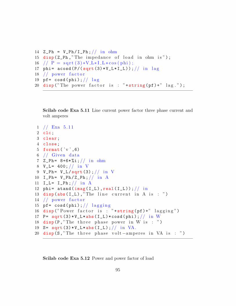
14 Z_Ph = V_Ph/I_Ph;// i n ohm15 disp(Z_Ph ,”The impedance o f l o ad i n ohm i s ”);16 // P = s q r t ( 3 ) ∗V L∗ I L ∗ co s ( ph i ) ;17 phi= acosd(P/(sqrt (3)*V_L*I_L));// i n l a g18 // power f a c t o r19 pf= cosd(phi);// l a g20 disp(”The power f a c t o r i s : ”+string(pf)+” l a g . ”);

Scilab code Exa 5.11 Line current power factor three phase current andvolt amperes

1 // Exa 5 . 1 12 clc;

3 clear;

4 close;

5 format( ’ v ’ ,6)6 // Given data7 Z_Ph= 8+6*%i;// i n ohm8 V_L= 400; // i n V9 V_Ph= V_L/sqrt (3);// i n V

10 I_Ph= V_Ph/Z_Ph;// i n A11 I_L= I_Ph;// i n A12 phi= atand(imag(I_L),real(I_L));// i n13 disp(abs(I_L),”The l i n e c u r r e n t i n A i s : ”)14 // power f a c t o r15 pf= cosd(phi);// l a g g i n g16 disp(”Power f a c t o r i s : ”+string(pf)+” l a g g i n g ”)17 P= sqrt (3)*V_L*abs(I_L)*cosd(phi);// i n W18 disp(P,”The t h r e e phase power i n W i s : ”)19 S= sqrt (3)*V_L*abs(I_L);// i n VA.20 disp(S,”The t h r e e phase vo l t−amperes i n VA i s : ”)

Scilab code Exa 5.12 Power and power factor of load

95

1 // Exa 5 . 1 22 clc;

3 clear;

4 close;

5 format( ’ v ’ ,7)6 // Given data7 W1 = 20; // i n kW8 W2 = -5; // i n kW9 P = W1+W2;// i n kW

10 disp(P,”The power i n kW i s : ”)11 phi = (atand( sqrt (3) *((W1 -W2)/(W1+W2)) ));// i n l a g12 // Power f a c t o r o f the l oad13 pf= cosd(phi)

14 disp(pf,”The power f a c t o r o f the l oad i s : ”);

Scilab code Exa 5.13 Reading of two wattmeters

1 // Exa 5 . 1 32 clc;

3 clear;

4 close;

5 format( ’ v ’ ,6)6 // Given data7 V_L = 400; // i n V8 I_L = 10; // i n A9 W2= 1; // assumed

10 W1= 2*W2;

11 phi= atand(sqrt (3)*(W1 -W2)/(W1+W2));

12 W1= V_L*I_L*cosd(30-phi);// i n W13 W2= V_L*I_L*cosd (30+ phi);// i n W14 disp(W1,”The r e a d i n g o f f i r s t wattmeter i n W i s : ”)15 disp(W2,”The r e a d i n g o f s econd wattmeter i n W i s : ”

)

96

Scilab code Exa 5.14 Phase current resistance and inductance of coil andpower drawn by coil

1 // Exa 5 . 1 42 clc;

3 clear;

4 close;

5 format( ’ v ’ ,6)6 // Given data7 V_L = 400; // i n V8 f = 50; // i n Hz9 I_L = 17.32; // i n A

10 phi = acosd (0.8);

11 I_Ph =I_L/sqrt (3);// i n A12 disp(I_Ph ,”The phase c u r r e n t i n A i s ”);13 V_Ph=V_L;// i n V14 Z_Ph = V_Ph/I_Ph;// i n ohm15 Z_Ph= Z_Ph*expm(phi*%i*%pi /180);// i n ohm16 R= real(Z_Ph);// i n ohm17 XL= imag(Z_Ph);// i n ohm18 L= XL/(2* %pi*f);// i n H19 L= L*10^3; // i n mH20 disp(R,”The r e s i s t a n c e o f the c o i l i n i s : ”)21 disp(L,”The i n d u c t a n c e o f the c o i l i n mH i s : ”)22 // The power drawn by each c o i l23 P_Ph= V_Ph*I_Ph*cosd(phi);// i n W24 disp(P_Ph ,”The power drawn by each c o i l i n W i s : ”)

Scilab code Exa 5.15 Reading of each wattmeter

1 // Exa 5 . 1 52 clc;

97

3 clear;

4 close;

5 format( ’ v ’ ,8)6 // Given data7 P = 30; // i n kW8 pf = 0.7;

9 // cosd ( ph i ) = p f ;10 phi = acosd(pf);// i n d e g r e e11 // P = s q r t ( 3 ) ∗V L∗ I L ∗ cosd ( ph i ) ;12 theta = 30; // i n d e g r e e13 V_LI_L = P/(sqrt (3)*cosd(phi));

14 W1 = V_LI_L*cosd(theta -phi);// i n kW15 disp(W1,”The r e a d i n g o f f i r s t wattmeter i n kW i s ”);16 W2 = V_LI_L*cosd(theta+phi);// i n kW17 disp(W2,”The r e a d i n g o f s econd wattmeter i n kW i s ”);

Scilab code Exa 5.16 Values and nature of load components and powerfactor

1 // Exa 5 . 1 62 clc;

3 clear;

4 close;

5 format( ’ v ’ ,7)6 // Given data7 P = 18; // i n kW8 P= P*10^3; // i n W9 I_L = 60; // i n A

10 V_L = 440; // i n V11 f= 50; // i n Hz12 // P = s q r t ( 3 ) ∗V L∗ I L ∗ cosd ( ph i ) ;13 phi= acosd(P/(sqrt (3)*V_L*I_L));// i n14 I_L= I_L*expm(phi*%pi*%i/180);// i n A15 I_Ph= I_L;// i n A16 V_Ph= V_L/sqrt (3);// i n V

98

17 Z_Ph= V_Ph/I_Ph;// i n ohm18 R= real(Z_Ph);// i n ohm19 XC=abs(imag(Z_Ph));// i n ohm20 C = 1/(2* %pi*f*XC);// i n F21 C=C*10^6; // i n F22 // Power f a c t o r23 pf= cosd(phi);// l e a d24 disp(”The power f a c t o r i s : ”+string(pf)+” l e a d i n g ”)25 disp(R,”The r e s i s t a n c e i n i s : ”)26 disp(C,”The c a p a c i t a n c e i n F i s : ”);27 disp(”The l oad i s c a p a c i t i v e i n na tu r e . ”)

Scilab code Exa 5.17 Line current impedance of each phase and resistanceand inductance of each phase

1 // Exa 5 . 1 72 clc;

3 clear;

4 close;

5 format( ’ v ’ ,7)6 // Given data7 V_L = 400; // i n V8 f = 50; // i n Hz9 W1 = 8000; // i n W

10 W2 = 4000; // i n W11 W = W1+W2;// i n W12 phi =( atand( sqrt (3)*((W1-W2)/(W1+W2)) ));// i n l a g13 P = W;// i n W14 //P = s q r t ( 3 ) ∗V L∗ I L ∗ cosd ( ph i ) ;15 I_L = P/(sqrt (3)*V_L*cosd(phi));// i n A16 V_Ph = V_L/sqrt (3);// i n V17 I_Ph = I_L;// i n A18 Z_Ph = V_Ph/I_Ph;// i n ohm19 Z_Ph= Z_Ph*expm(phi*%i*%pi /180);// ohm20 R_Ph= real(Z_Ph);// i n ohm

99

21 XL_Ph= imag(Z_Ph);// i n ohm22 L_Ph= XL_Ph /(2* %pi*f);// i n H23 // power f a c t o r24 pf= cosd(phi);

25 disp(pf,”The power f a c t o r i s : ”)26 disp(I_L ,”The l i n e c u r r e n t i n A i s ”);27 disp(Z_Ph ,”The impedance o f each phase i n i s : ”)28 disp(R_Ph ,”The r e s i s t a n c e o f each phase i n i s : ”

)

29 disp(L_Ph ,”The i n d u c t a n c e o f each phase i n H i s : ”)

100

Chapter 6

Measuring Instruments

Scilab code Exa 6.1 Required shunt resistance

1 // Exa 6 . 12 clc;

3 clear;

4 close;

5 format( ’ v ’ ,6)6 // Given data7 Rm = 8; // i n ohm8 Im = 20; // i n mA9 Im = Im * 10^ -3; // i n A

10 I = 1; // i n A11 // M u l t i p l y i n g f a c t o r12 N = I/Im;

13 // Shunt r e s i s t a n c e14 Rsh = Rm/(N-1);// i n ohm15 disp(Rsh ,”The shunt r e s i s t a n c e r e q u i r e d i n i s ”);

Scilab code Exa 6.2 Multiplying factor

101

1 // Exa 6 . 22 clc;

3 clear;

4 close;

5 format( ’ v ’ ,6)6 // Given data7 Rm = 6; // i n ohm8 Rsh = 0.025; // i n ohm9 N = 1 + (Rm/Rsh);// m u l t i p l y i n g f a c t o r

10 disp(N,”The m u l t i p l y i n g f a c t o r i s ”);

Scilab code Exa 6.3 Resistance to be connected in parallel and series

1 // Exa 6 . 32 clc;

3 clear;

4 close;


10 I = 1; // i n A11 N = I/Im;// m u l t i p l y i n g f a c t o r12 Rsh = Rm/(N-1);// i n ohm13 disp(Rsh ,”The r e s i a t n c e to be connec t ed i n p a r a l l e l

i n i s ”);14 V = 10; // i n V15 Rs = (V/Im)-Rm;// i n ohm16 disp(Rs,”The r e s i a t n c e to be connec t ed i n s e r i e s i n

i s ”);

Scilab code Exa 6.4 Current range

102

1 // Exa 6 . 42 clc;

3 clear;

4 close;

5 format( ’ v ’ ,5)6 // Given data7 V=250; // f u l l s c a l e v o l t a g e r e a d i n g i n V8 Rm = 2; // i n ohm9 Rsh = 2; // i n m ohm

10 Rsh = Rsh * 10^-3; // i n ohm11 R = 5000; // i n ohm12 Im = V/(Rm+R);// i n A13 Ish = (Im*Rm)/Rsh;// i n A14 // Current range o f i n s t rument15 I = Im+Ish;// i n A16 disp(I,”The c u r r e n t range o f i n s t rument i n A i s ”);

Scilab code Exa 6.5 Percentage error

1 // Exa 6 . 52 clc;

3 clear;

4 close;

5 format( ’ v ’ ,6)6 // Given data7 V = 230; // i n V8 I = 35; // i n A9 N = 200;

10 t = 64; // i n s e c11 kwh = 500;

12 phi= acosd (0.8);// i n13 Er = N/kwh;// i n kWh14 Et = V*I*cosd(phi)*t;// i n J o u l e s15 Et = Et /3600; // i n W hour16 Et = Et * 10^ -3; // i n kWh

103

17 // p e r c e n t a g e e r r o r18 PerError = ((Er -Et)/Et)*100; // i n %19 disp(PerError ,”The p e r c e n t a g e e r r o r i n % i s ”);


1 // Exa 6 . 62 clc;

3 clear;

4 close;

5 format( ’ v ’ ,6)6 // Given data7 I = 50; // i n A8 V = 230; // i n V9 N = 61;

10 t = 37; // i n s e c11 KWh = 500;

12 phi= acosd (1);// i n13 Er = N/KWh;// i n kWh14 Et = V*I*cosd(phi)*t;// i n J o u l e s15 Et = Et /3600; // i n Wh16 Et = Et*10^ -3; // i n kWh17 // Pe r c en tage e r r o r18 PerError = ((Er -Et)/Et)*100; // i n %19 disp(PerError ,”The p e r c e n t a g e e r r o r i n % i s ”);

Scilab code Exa 6.7 Series resistance

1 // Exa 6 . 72 clc;

3 clear;

4 close;

5 format( ’ v ’ ,9)

104

6 // Given data7 Im = 20; // i n mA8 Im = Im * 10^-3; // i n A9 Vm = 50; // i n mV

10 Vm = Vm * 10^ -3; // i n V11 V = 500; // i n V12 Rm = Vm/Im;// i n ohm13 Rs = (V/Im)-Rm;// i n ohm14 disp(Rs,”The s e r i e s r e s i s t a n c e i n ohm i s ”);

Scilab code Exa 6.8 Value of Rs and Rsh

1 // Exa 6 . 82 clc;

3 clear;

4 close;


10 V = 100; // i n V11 Rs = (V/Im)-Rm;// i n ohm12 disp(Rs,”The v a l u e o f Rs i n i s ”);13 N = 1/Im;

14 Rsh = Rm/(N-1);// i n ohm15 disp(Rsh ,”The v a l u e o f Rsh i n i s ”);


1 // Exa 6 . 92 clc;

3 clear;

105

4 close;

5 format( ’ v ’ ,5)6 // Given data7 I = 40; // i n A8 V = 230; // i n V9 N = 600;

10 t = 46; // i n s e c11 phi= acosd (1);// i n12 P = V*I*cosd(phi);// i n W13 P = P * 10^-3; // i n kW14 // 1 kWh = 500 r e v o l u t i o n15 P = P * 500; // i n r e v o l u t i o n16 T = (3600/t)*60; // i n r e v o l u t i o n17 // Pe r c en tage e r r o r18 PerError = ((T-P)/P)*100; // i n %19 disp(PerError ,”The p e r c e n t a g e e r r o r i n % i s ”);

Scilab code Exa 6.10 Number of revolution

1 // Exa 6 . 1 02 clc;

3 clear;

4 close;

5 format( ’ v ’ ,6)6 // Given data7 N = 100;

8 I = 20; // i n A9 V = 210; // i n V

10 pf = 0.8; // i n l a d11 Er = 350; // i n r ev12 a = 3.36; // assumed13 Et = (a*3600) /3600; // i n kWh14 // 1 kWh = 1 0 0 ; / / r e v o l u t i o n15 Et = Et*N;// r e v o l u t i o n16 // Pe r c en tage e r r o r

106

17 PerError = ((Er -Et)/Et)*100; // i n %18 disp(PerError ,”The p e r c e n t a g e e r r o r i n % i s ”);


1 // Exa 6 . 1 12 clc;

3 clear;

4 close;

5 format( ’ v ’ ,6)6 // Given data7 I = 5; // i n A8 V = 230; // i n V9 N = 61; // number o f r e v o l u t i o n

10 t = 37; // i n s e c11 // speed o f the d i s c12 discSpeed= 500; // i n r ev /kWh13 Er = N/discSpeed;

14 Et = (V*I*t)/(3600*100);

15 // p e r c e n t a g e e r r o r16 PerError = ((Er -Et)/Et)*100; // i n %17 disp(PerError ,”The p e r c e n t a g e e r r o r i n % i s ”);

107

Chapter 8

Magnetic Circuits

Scilab code Exa 8.1 Required current

1 // Exa 8 . 12 clc;

3 clear;

4 close;

5 format( ’ v ’ ,6)6 // Given data7 a = 3; // i n cmˆ28 a = a * 10^-4; // i n mˆ29 d = 20; // i n cm

10 N = 500;

11 phi = 0.5*10^ -3; // i n Wb12 miu_r = 833.33;

13 miu_o = 4*%pi *10^ -7;

14 l = %pi*d;// i n cm15 l = l * 10^-2; // i n m16 S = l/(miu_o*miu_r*a);// i n AT/Wb17 // C a l c u l a t i o n o f the c u r r e n t with the he lp o f f l u x18 // Formula ph i = (m∗m∗ f ) /S = (N∗ I ) /S ;19 I = (phi*S)/N;// i n A20 disp(I,”The c u r r e n t i n A i s ”);

108

Scilab code Exa 8.2 Coil mmf field strength total flux reluctance and per-meance of the ring

1 // Exa 8 . 22 clc;

3 clear;

4 close;


8 miu_r = 900;

9 l = 40; // i n cm10 a = 5; // i n cmˆ211 R = 100; // i n ohm12 V = 250; // i n V13 miu_o = 4*%pi *10^ -7;

14 I = V/R;// i n A15 mmf = N*I;// i n AT16 disp(mmf ,”The c o i l mmf i n AT i s ”);17 H = (N*I)/(l*10^ -2);// i n AT/m18 disp(H,”The f i e l d s t r e n g t h i n AT/m i s ”);19 B = miu_o*miu_r*H;// i n Wb/mˆ220 phi = B*a*10^ -4; // i n Wb21 disp(phi ,” Tota l f l u x i n Wb i s ”);22 S = mmf/phi;// i n AT/Wb23 disp(S,”The r e l u c t a n c e o f the r i n g i n AT/Wb i s ”);24 // Permeance i s r e c i p o c a l o f r e l u c t a n c e25 Permeance = 1/S;// i n Wb/AT26 disp(Permeance ,” Permeance o f the r i n g i n Wb/AT i s ”);

Scilab code Exa 8.3 Ampere turns

109

1 // Exa 8 . 32 clc;

3 clear;

4 close;

5 format( ’ v ’ ,6)6 // Given data7 Ig = 4; // i n mm8 Ig = Ig * 10^ -3; // i n m9 B = 1.3; // i n Wb/mˆ2

10 miu_r = 1;

11 miu_o = 4*%pi *10^ -7;

12 H = B/( miu_o*miu_r);// i n AT/m13 Hg = H;// i n AT/m14 // Ampere turn r e q u i r e d f o r a i r gap15 AT = Hg*Ig;// AT f o r a i r gap i n AT16 disp(AT,”The amphere t u r n s f o r the gap i n AT i s ”);

Scilab code Exa 8.4 Total flux in the ring

1 // Exa 8 . 42 clc;

3 clear;

4 close;


8 R = 4; // i n ohm9 d = 0.25; // i n m

10 a = 700; // i n mmˆ211 a = a*10^ -6; // i n mˆ212 V = 6; // i n V13 miu_r = 550;

14 miu_o = 4*%pi *10^ -7;

15 // E v a l u a t i o n o f c u r r e n t by ohm ’ s law16 I = V/R;// i n A

110

17 l = %pi*d;// i n m18 H = (N*I)/l;// i n A/m19 // E v a l u a t i o n o f f l u x d e n s i t y20 B = miu_o*miu_r*H;// i n T21 // E v a l u a t i o n o f t o t a l f l u x22 phi = B*a;// i n Wb23 phi= phi *10^3; // i n mWb24 disp(phi ,”The t o t a l f l u x i n the c o i l i n m/Wb i s ”);

Scilab code Exa 8.5 MMF total reluctance flux and flux density of thering

1 // Exa 8 . 52 clc;

3 clear;

4 close;

5 format( ’ v ’ ,8)6 // Given data7 d_r = 8; // d iamete r o f r i n g i n cm8 d_r = d_r *10^ -2; // i n m9 d_i = 1; // d iamete r o f i r o n i n cm

10 d_i = d_i * 10^-2; // i n m11 Permeability = 900;

12 gap = 2; // i n mm13 gap = gap * 10^-3; // i n m14 N = 400;

15 I = 3.5; // i n A16 l_i = (%pi*d_r)-gap;// l e n g t h o f i r o n i n m17 a = (%pi/4)*(d_i^2);// i n mˆ218 mmf = N*I;// i n AT19 disp(mmf ,”The mmf i n AT i s ”);20 miu_o = 4*%pi *10^ -7;

21 miu_r = 900;

22 Si = l_i/(miu_o*miu_r*a);// i n AT/Wb23 miu_r = 1;

111

24 Sg = gap/(miu_o*miu_r*a);// i n AT/Wb25 S_T = Si+Sg;// i n AT/Wb26 disp(S_T ,”The t o t a l r e l u c t a n c e i n AT/Wb i s ”);27 phi = mmf/S_T;// i n Wb28 disp(phi ,”The f l u x i n Wb i s ”);29 // ph i = B∗a ;30 B = phi/a;// i n Wb/mˆ231 disp(B,”The f l u x d e n s i t y o f the r i n g i n Wb/mˆ2 ”);

Scilab code Exa 8.6 Reluctance of magnetic circuit and inductance of coil

1 // Exa 8 . 62 clc;

3 clear;

4 close;

5 format( ’ v ’ ,8)6 // Given data7 miu_r = 1400;

8 l = 70; // i n cm9 l = l * 10^-2; // i n m

10 a = 5; // i n cmˆ211 a = a * 10^-4; // i n mˆ212 N = 1000;

13 miu_o = 4*%pi *10^ -7;

14 S = l/(miu_o*miu_r*a);// i n AT/Wb15 disp(S,”The r e l u c t a n c e o f the magnet i c c i r c u i t i n AT

/Wb i s ”);16 format( ’ v ’ ,7)17 // C a l c u l a t i o n o f i n d u c t a n c e o f the c o i l18 L = (N^2)/S;// i n H19 disp(L,”The i n d u c t a n c e o f the c o i l i n H i s ”);2021 // Note : In the book the c a l c u l a t e d v a l u e o f L i s

c o r r e c t but at l a s t they p r i n t i t s v a l u e wrong

112


1 // Exa 8 . 72 clc;

3 clear;

4 close;

5 format( ’ v ’ ,7)6 // Given data7 l1 = 25; // i n cm8 l1 = l1 * 10^ -2; // i n m9 miu_o = 4*%pi *10^ -7;

10 miu_r = 750;

11 a1 = 2.5*2.5*10^ -4; // i n m12 S1 = l1/(miu_o*miu_r*a1);// i n AT/Wb13 l2 = 40; // i n cm14 l2 = l2 * 10^ -2; // i n m15 S2 = l2/(miu_o*miu_r*a1);// i n AT/Wb16 phi2 = 2.5*10^ -3; // i n Wb17 N = 500;

18 //mmf = phi1 ∗S1 = phi2 ∗S2 ;19 phi1 = (phi2*S2)/S1;// i n Wb20 phi = phi1+phi2;// i n Wb21 // Sum o f mmf r e q u i r e d f o r AEFB22 S_AEFB = S2;// i n AT/Wb23 mmfforAEFB = S_AEFB*phi;//mmf f o r AEFB i n AT24 totalmmf = mmfforAEFB +(phi1*S1);// t o t a l mmf i n AT25 // N∗ I = tota lmmf ;26 // C a l c u l a t i o n o f c u r r e n t27 I = totalmmf/N;// i n A28 disp(I,”The c u r r e n t i n A i s ”);

Scilab code Exa 8.8 Exciting current needed in a coil

113

1 // Exa 8 . 82 clc;

3 clear;

4 close;

5 format( ’ v ’ ,6)6 // Given data7 a = 16*10^ -4; // i n mˆ28 lg = 2*10^ -3; // i n m9 N = 1000;

10 phi = 4*10^ -3; // i n Wb11 miu_r = 2000;

12 miu_o = 4*%pi *10^ -7;

13 l=25; // l e n g t h o f magnet i c i n cm14 w= 20; // i n cm ( width )15 t= 4; // i n cm ( t h i c k n e s s )16 li= {[w-t]*t/2+[l-t]*t/2 -0.2}; // i n cm17 li= li*10^ -2; // i n m18 S_T= 1/( miu_o*a)*(li/miu_r+lg)

19 // C a l c u l a t i o n o f c u r r e n t with the he lp o f f l u x20 // ph i = mmf/S T = N∗ I /S T ;21 I = (phi*S_T)/N;// i n A22 disp(I,”The c u r r e n t i n A i s ”);

Scilab code Exa 8.9 Total flux in the ring

1 // Exa 8 . 92 clc;

3 clear;

4 close;


8 R = 4; // i n ohm9 d_mean = 0.25; // i n m

10 a = 700; // i n mmˆ2

114

11 a = a * 10^-6; // i n m12 V = 6; // i n V13 miu_r = 550;

14 miu_o = 4*%pi *10^ -7;

15 l_i = %pi*d_mean;// i n m16 S = l_i/( miu_o*miu_r*a);// i n AT/Wb17 I = V/R;// i n A18 // C a l c u l a t i o n o f mmf19 mmf = N*I;// i n AT20 // t o t a l f l u x21 phi = mmf/S;// i n Wb22 phi = phi * 10^6; // i n W b23 disp(phi ,”The t o t a l f l u x i n the r i n g i n W b i s ”);2425 // Note : In the book the v a l u e o f f l u x c a l c u l a t e d

c o r r e c t i n W b but at l a s t they p r i n t on ly i n Wb, so the answer i n the book i s wrong .

Scilab code Exa 8.10 Coil inductance

1 // Exa 8 . 1 02 clc;

3 clear;

4 close;


8 a = 5; // i n cmˆ29 a = a * 10^-4; // i n mˆ2

10 l_g = 2; // i n mm11 l_g = l_g * 10^-3; // i n m12 B = 0.5; // i n T13 miu_r= %inf;

14 phi = B*a;// i n Wb15 miu_o = 4*%pi *10^ -7;

115

16 S = l_g/( miu_o*a);// i n AT/Wb17 // C a l c u l a t i o n o f c u r r e n t with the he lp o f f l u x18 // ph i = mmf/S = N∗ I /S ;19 I = (phi*S)/N;// i n A20 disp(I,”The c u r r e n t r e q u i r e d i n A i s ”);21 // E v a l u a t i o n o f c o i l i n d u c t a n c e22 L = (N^2)/S;// i n H23 disp(L,”The c o i l i n d u c t a n c e i n H i s ”);

Scilab code Exa 8.11 Ampere turns

1 // Exa 8 . 1 12 clc;

3 clear;

4 close;

5 format( ’ v ’ ,8)6 // Given data7 l_g = 4; // i n mm8 l_g = l_g * 10^-3; // i n m9 Bg = 1.3; // i n Wb/mˆ2

10 miu_o = 4*%pi *10^ -7;

11 Hg = Bg/miu_o;

12 // Ampere t u r n s f o r the gap13 AT = Hg*l_g;// i n AT14 disp(AT,”The amphere t u r n s i n AT i s ”);

Scilab code Exa 8.12 Required MMF

1 // Exa 8 . 1 22 clc;

3 clear;

4 close;

5 format( ’ v ’ ,6)

116

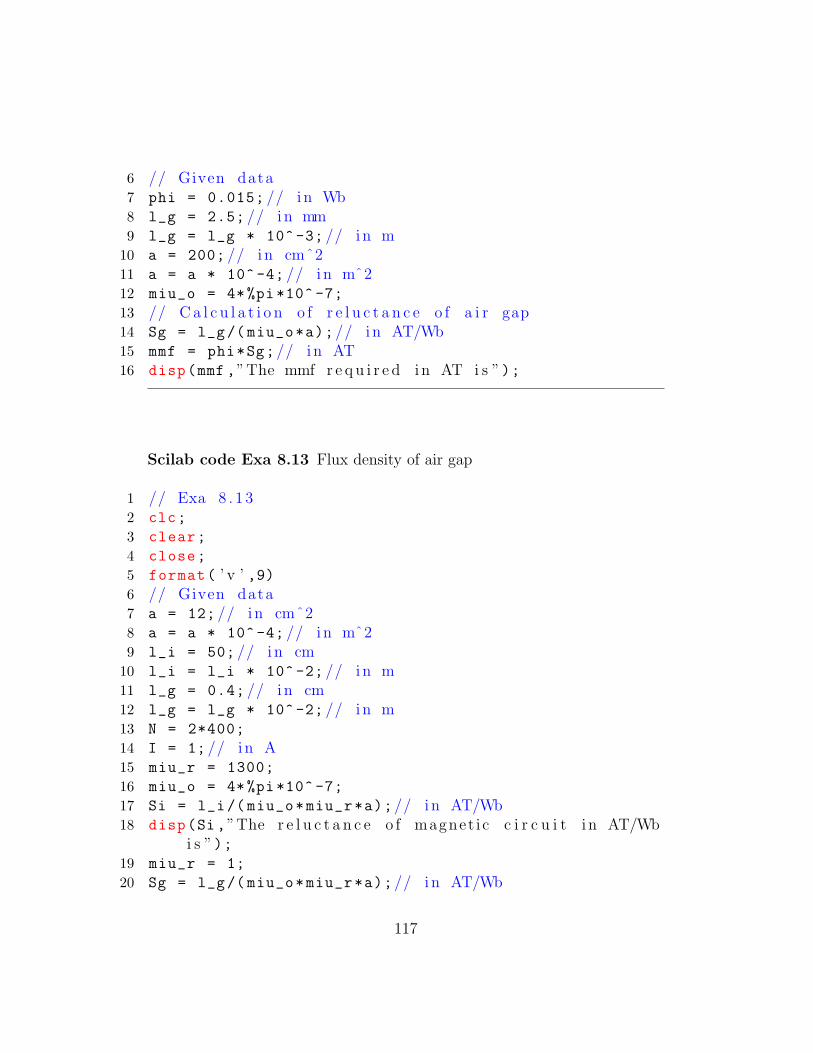
6 // Given data7 phi = 0.015; // i n Wb8 l_g = 2.5; // i n mm9 l_g = l_g * 10^-3; // i n m

10 a = 200; // i n cmˆ211 a = a * 10^-4; // i n mˆ212 miu_o = 4*%pi *10^ -7;

13 // C a l c u l a t i o n o f r e l u c t a n c e o f a i r gap14 Sg = l_g/(miu_o*a);// i n AT/Wb15 mmf = phi*Sg;// i n AT16 disp(mmf ,”The mmf r e q u i r e d i n AT i s ”);

Scilab code Exa 8.13 Flux density of air gap

1 // Exa 8 . 1 32 clc;

3 clear;

4 close;

5 format( ’ v ’ ,9)6 // Given data7 a = 12; // i n cmˆ28 a = a * 10^-4; // i n mˆ29 l_i = 50; // i n cm

10 l_i = l_i * 10^-2; // i n m11 l_g = 0.4; // i n cm12 l_g = l_g * 10^-2; // i n m13 N = 2*400;

14 I = 1; // i n A15 miu_r = 1300;

16 miu_o = 4*%pi *10^ -7;

17 Si = l_i/(miu_o*miu_r*a);// i n AT/Wb18 disp(Si,”The r e l u c t a n c e o f magnet i c c i r c u i t i n AT/Wb

i s ”);19 miu_r = 1;

20 Sg = l_g/(miu_o*miu_r*a);// i n AT/Wb

117

21 disp(Sg,”The r e l u c t a n c e o f a i r gap i n AT/Wb i s ”);22 S_T = Si+Sg;// i n AT/Wb23 disp(S_T ,” Tota l r e l u c t a n c e i n AT/Wb i s ”);24 format( ’ v ’ ,7)25 mmf = N*I;// i n AT26 phi_T = mmf/S_T;// i n Wb27 phi_T= phi_T *10^3; // i n mWb28 disp(phi_T ,”The t o t a l f l u x i n mWb i s ”);29 phi_T= phi_T *10^ -3; // i n Wb30 // phi T =B∗a ;31 B = (phi_T)/a;// i n Wb/mˆ232 disp(B,”The f l u x d e n s i t y o f a i r gap i n Wb/mˆ2 i s ”);


1 // Exa 8 . 1 42 clc;

3 clear;

4 close;

5 format( ’ v ’ ,7)6 // Given data7 l = 30; // i n cm8 d = 2; // i n cm9 N = 500;

10 phi = 0.5; // i n mWb11 Airgap = 1; // i n mm12 miu_r = 4000;

13 miu_o = 4*%pi *10^ -7;

14 Ac = (%pi/4)*(d^2);// i n cmˆ215 Ac = Ac * 10^ -4; // i n mˆ216 l_i = (l*10^ -2) -(Airgap *10^ -3);// i n m17 l_g = 1; // i n mm18 l_g = l_g * 10^-3; // i n m19 Si = l_i/(miu_r*miu_o*Ac);// i n AT/Wb20 Sg = l_g/(miu_o*Ac);// i n AT/Wb

118

21 S =Si+Sg;// i n AT/Wb22 // ph i = mmf/S = N∗ I /S ;23 I = (phi *10^ -3*S)/N;// i n A24 disp(I,”The c u r r e n t r e q u i r e d i n A i s ”);

Scilab code Exa 8.15 Coil inductance

1 // Exa 8 . 1 52 clc;

3 clear;

4 close;

5 format( ’ v ’ ,7)6 // Given data7 l = 40; // i n cm8 l = l * 10^-2; // i n m9 a = 4; // i n cmˆ2

10 a = a * 10^-4; // i n mˆ211 miu_r = 1000;

12 miu_o = 4*%pi *10^ -7;

13 l_g = 1; // i n mm14 l_g = l_g * 10^-3; // i n m15 N = 1000;

16 l_i = l-l_g;// i n m17 Si = l_i/(miu_r*miu_o*a);// i n AT/Wb18 Sg = l_g/(miu_o*a);// i n AT/Wb19 S = Si+Sg;// i n AT/Wb20 // The i n d u c t n a c e o f the c o i l21 L = (N^2)/S;// i n H22 disp(L,”The i n d u c t n a c e o f the c o i l i n H i s ”);

119

Chapter 9

Single Phase Transformer

Scilab code Exa 9.1 Primary turns primary and secondary full load cur-rent

1 // Exa 9 . 12 clc;

3 clear;

4 close;

5 format( ’ v ’ ,6)6 // Given data7 V1 = 3000; // i n V8 V2 = 300; // i n V9 N2 = 86; // i n Turns

10 Rating = 60*10^3; // i n VA11 K = V2/V1;

12 // Trans fo rmer r a t i o , N2/N1 = K;13 N1 = N2/K;// i n t u r n s14 disp(N1,”The numbers o f pr imary t u r n s i s ”);15 I2 = Rating/V2;// i n A16 disp(I2,”The s e condary f u l l l o ad c u r r e n t i n A i s ”);17 I1 = Rating/V1;// i n A18 disp(I1,”The pr imary f u l l l o ad c u r r e n t i n A i s ”);

120

Scilab code Exa 9.2 Maximum flux density

1 // Exa 9 . 22 clc;

3 clear;

4 close;

5 format( ’ v ’ ,5)6 // Given data7 E1 = 3000; // i n V8 E2 = 200; // i n V9 f = 50; // i n Hz

10 a = 150; // i n cmˆ211 N2 = 80; // t u r n s12 // Formula E2 = 4 . 4 4∗ phi m ∗ f ∗N2 ;13 phi_m = E2 /(4.44*f*N2);// i n Wb14 Bm = phi_m/(a*10^ -4);// i n Wb/mˆ215 disp(Bm,”The maximum f l u x d e n s i t y i n Wb/mˆ2 i s ”);

Scilab code Exa 9.3 Maximum core flux

1 // Exa 9 . 32 clc;

3 clear;

4 close;

5 format( ’ v ’ ,5)6 // Given data7 N1 = 500;

8 N2 = 40;

9 E1 = 3000; // i n V10 f = 50; // i n Hz11 K = N2/N1;

12 Rating = 25*10^3; // i n VA

121

13 I1 = Rating/E1;// i n A14 disp(I1,”The pr imary f u l l l o ad c u r r e n t i n A i s ”);15 I2 = I1/K;// i n A16 disp(I2,”The s e condary f u l l l o ad c u r r e n t i n A i s ”);17 // K = E2/E1 ;18 E2 = K*E1;// i n V19 disp(E2,”The s e condary emf i n V i s ”);20 // e .m. f e q u a t i o n o f the t r a n s f o r m e r , E1 = 4 . 4 4∗

phi m ∗ f ∗N1 ;21 phi_m = E1 /(4.44*f*N1);// i n Wb22 phi_m = phi_m *10^3; // i n mWb23 disp(phi_m ,”The maximum c o r e f l u x i n mWb i s ”);

Scilab code Exa 9.4 Two component of current

1 // Exa 9 . 42 clc;

3 clear;

4 close;

5 format( ’ v ’ ,6)6 // Given data7 Rating = 25; // i n KVA8 f = 50; // i n Hz9 Io = 15; // i n A

10 Wo = 350; // i n W11 Vo = 230; // i n V12 // No load power f a c t o r13 phi_o = acosd(Wo/(Vo*Io));

14 // a c t i v e component o f c u r r e n t15 Ic = Io*cosd(phi_o);// i n A16 disp(Ic,”The a c t i v e component o f c u r r e n t i n A i s ”);17 // magne t i z i ng component o f c u r r e n t18 Im = Io*sind(phi_o);// i n A19 disp(Im,”The magne t i z i ng component o f c u r r e n t i n A

i s ”);

122

Scilab code Exa 9.5 Equivalent Resistance reactance and impedence ref-fered to primary and secondary

1 // Exa 9 . 52 clc;

3 clear;

4 close;

5 format( ’ v ’ ,8)6 // Given data7 V1 = 2200; // i n V8 V2 = 110; // i n V9 R1 = 1.75; // i n ohm

10 R2 = 0.0045; // i n ohm11 X1 = 2.6; // i n ohm12 X2 = 0.0075; // i n ohm13 K = V2/V1;

14 // R1e = R1+R 2 = R1 + (R2/(Kˆ2) ) ;15 R1e = R1 + (R2/(K^2));// i n ohm16 disp(R1e ,” E q u i v a l e n t r e s i s t a n c e r e f f e r e d to pr imary

i n ohm i s ”);17 // R2e = R2+R 1 = R2+((Kˆ2) ∗R1) ;18 R2e = R2+((K^2)*R1);// i n ohm19 disp(R2e ,” E q u i v a l e n t r e s i s t a n c e r e f f e r e d to

s e condary i n ohm i s ”);20 //X1e = X1+X 2 = X1+(X2/(Kˆ2) ) ;21 X1e = X1+(X2/(K^2));// i n ohm22 disp(X1e ,” E q u i v a l e n t r e a c t a n c e r e f f e r e d to pr imary

i n ohm i s ”);23 // X2e = X2+X 1 = X2 + ( (Kˆ2) ∗X1) ;24 X2e = X2 + ((K^2)*X1);// i n ohm25 disp(X2e ,” E q u i v a l e n t r e a c t a n c e r e f f e r e d to s e conda ry

i n ohm i s ”);26 Z1e= R1e+%i*X1e;// i n ohm27 Z2e= R2e+%i*X2e;// i n ohm

123

28 disp(abs(Z1e),” E q u i v a l e n t impedance r e f f e r e d topr imary i n ohm i s : ”)

29 disp(abs(Z2e),” E q u i v a l e n t impedance r e f f e r e d tos e condary i n ohm i s : ”)

Scilab code Exa 9.6 Total copper loss

1 // Exa 9 . 62 clc;

3 clear;

4 close;

5 format( ’ v ’ ,7)6 // Given data7 V1 = 2200; // i n V8 V2 = 440; // i n V9 R1 = 0.3; // i n ohm

10 R2 = 0.01; // i n ohm11 X1 = 1.1; // i n ohm12 X2 = 0.035; // i n ohm13 K = V2/V1;

14 Rating = 100; // i n KVA15 I1 = (Rating *10^3)/V1;// i n A16 I2 = (Rating *10^3)/V2;// i n A17 R1e = R1 + (R2/(K^2));// i n ohm18 X1e = X1+(X2/(K^2));// i n ohm19 Z1e = sqrt( (R1e^2) + (X1e ^2) );// i n ohm20 disp(Z1e ,”The e q u i v a l e n t impedance o f the

t r a n s f o r m e r r e f f e r e d to pr imary i n ohm i s ”);21 // Tota l copper l o s s22 totalcopperloss = (I1^2)*R1e;// i n W23 disp(totalcopperloss ,”The t o t a l copper l o s s i n W i s ”

);

124

Scilab code Exa 9.7 Efficiency of transformer

1 // Exa 9 . 72 clc;

3 clear;

4 close;

5 format( ’ v ’ ,6)6 // Given data7 Rating = 150000; // i n VA8 phi= acosd (0.8);// i n9 Pcu = 1600; // i n W

10 Pi = 1400; // i n W11 n = 1/4;

12 // Tota l l o s s o f 25% load13 totalloss = Pi + (n^2)*Pcu;// i n W14 // e f f i c i e n c y o f t r a n s f o r m e r o f 25% load15 Eta = n*Rating*cosd(phi)/(n*Rating*cosd(phi)+Pi+n^2*

Pcu)*100; // i n %16 disp(Eta ,”The e f f i c i e n c y i n % i s ”);

Scilab code Exa 9.8 Efficiency on unity power factor

1 // Exa 9 . 82 clc;

3 clear;

4 close;

5 format( ’ v ’ ,6)6 // Given data7 Rating = 25; // i n KVA8 V1 = 2000; // i n V9 V2 = 200; // i n V

10 Pi = 350; // i n W11 Pi = Pi * 10^ -3; // i n kW12 Pcu = 400; // i n W13 Pcu = Pcu * 10^-3; // i n kW

125

14 phi= acosd (1);// i n15 output = Rating;

16 losses = Pi+Pcu;

17 Eta = (output /( output + losses))*100; // %Eta i n %18 disp(Eta ,”The e f f i c i e n c y o f f u l l l o ad power i n % i s ”

);

19 // For h a l f l o ad20 output = Rating /2; // i n kW21 h = 1;

22 Pcu = Pcu*((h/2) ^2);// i n kW23 losses = Pi+Pcu;

24 // e f f i c i e n c y o f h a l f l o ad power25 Eta = (output /( output+losses))*100; // i n %26 disp(Eta ,”The e f f i c i e n c y o f h a l f l o ad power i n % i s ”

);

Scilab code Exa 9.9 Maximum efficiency

1 // Exa 9 . 92 clc;

3 clear;

4 close;

5 format( ’ v ’ ,7)6 // Given data7 Rating = 250*10^3; // i n VA8 Pi = 1.8; // i n kW9 Pi = Pi * 10^3; // i n W

10 Pcu_f1 = 2000; // i n W11 phi= acosd (0.8);// i n12 Eta = (( Rating*cosd(phi))/(( Rating*cosd(phi))+Pi+

Pcu_f1))*100; // %Eta i n %13 disp(Eta ,”The e f f i c i e n c y at f u l l l o ad i n % i s ”);14 // The maximum e f f i c i e n c y15 Eta_max = Rating * sqrt(Pi/Pcu_f1 );// i n VA16 Eta_max = Eta_max *10^ -3; // i n kVA

126

17 disp(Eta_max ,”The maximum e f f i c i e n c y i n kVA i s ”);18 Eta_max = Eta_max *10^3; // i n VA19 Pcu = Pi;// i n W20 Eta_max1 = (( Eta_max*cosd(phi))/(( Eta_max*cosd(phi))

+ Pi+Pcu ))*100; // i n %21 disp(Eta_max1 ,”The maximum e f f i c i e n c y i n % i s ”);

Scilab code Exa 9.10 Iron and full load copper loss

1 // Exa 9 . 1 02 clc;

3 clear;

4 close;

5 format( ’ v ’ ,9)6 // Given data7 phi= acosd (1);// i n8 Pout = 500; // i n kW9 Pout = Pout *10^3; // i n W

10 Eta = 90; // i n %11 n=1/2;

12 // For f u l l load , Eta= Pout ∗100/( Pout+Pi+Pcu f1 ) orPi+Pcu f1= ( Pout∗100−Eta∗Pout ) / Eta

( i )13 // For h a l f load , Eta= n∗Pout ∗100/( n∗Pout+Pi+nˆ2∗

Pcu f1 ) or Pi+nˆ2∗ Pcu f1= ( n∗Pout∗100−n∗Eta∗Pout )/ Eta ( i i )

14 // From eq ( i ) and ( i i )15 Pcu_fl= [(n*Pout *100-n*Eta*Pout)/Eta -(Pout *100-Eta*

Pout)/Eta]/(n^2-1)

16 Pi=(Pout *100-Eta*Pout)/Eta -Pcu_fl

17 disp(Pi,”The i r o n l o s s i n W i s : ”)18 disp(Pcu_fl ,”The f u l l l o ad copper l o s s i n watt ”)

127

Scilab code Exa 9.11 Maximum core flux

1 // Exa 9 . 1 12 clc;

3 clear;

4 close;

5 format( ’ v ’ ,6)6 // Given data7 Io = 10; // i n A8 phi_o= acosd (0.25);// i n9 V1 = 400; // i n V

10 f = 50; // i n Hz11 N1 =500;

12 Im = Io*sind(phi_o);// i n A13 disp(Im,”The magne t i z i ng component o f no l oad

c u r r e n t i n A i s ”);14 Pi = V1*Io*cosd(phi_o);// i n W15 disp(Pi,”The i r o n l o s s i n W i s ”);16 E1 = V1;// i n V17 //E1 v= 4 . 4 4∗ f ∗phi m ∗N1 ;18 phi_m = E1 /(4.44*f*N1);// i n Wb19 phi_m=phi_m *10^3; // i n mWb20 disp(phi_m ,”The maximum v a l u e o f f l u x i n mWb i s ”);

Scilab code Exa 9.12 Total copper loss

1 // Exa 9 . 1 22 clc;

3 clear;

4 close;

5 format( ’ v ’ ,6)6 // Given data7 Rating = 30*10^3; // i n VA8 V1 = 2000; // i n V9 V2 = 200; // i n V

128

10 f = 50; // i n Hz11 R1 = 3.5; // i n ohm12 X1 = 4.5; // i n ohm13 R2 = 0.015; // i n ohm14 X2 = 0.02; // i n ohm15 K = V2/V1;

16 R1e = R1 + (R2/(K^2));// i n ohm17 disp(R1e ,”The e q u i v a l e n t r e s i s t a n c e to pr imary s i d e

i n ohm i s ”);18 X1e = X1 + (X2/(K^2));// i n ohm19 disp(X1e ,”The e q u i v a l e n t r e a c t a n c e to pr imary s i d e

i n ohm i s ”);20 Z1e = sqrt( (R1e^2) + (X1e ^2) );// i n ohm21 disp(Z1e ,”The e q u i v a l e n t impedance to pr imary s i d e

i n ohm i s ”);22 I1 = Rating/V1;// i n A23 // Tota l copper l o s s i n t r a n s f o r m e r24 Pcu_total = (I1^2)*R1e;// i n W25 disp(Pcu_total ,” Tota l copper l o s s i n W i s ”);

Scilab code Exa 9.13 Secondary voltage at full load

1 // Exa 9 . 1 32 clc;

3 clear;

4 close;

5 format( ’ v ’ ,7)6 // Given data7 Rating = 10; // i n KVA8 phi= acosd (0.8)

9 V1 = 2000; // i n V10 V2 = 400; // i n V11 R1 = 5.5; // i n ohm12 X1 = 12; // i n ohm13 R2 = 0.2; // i n ohm

129

14 X2 = 0.45; // i n ohm15 K = V2/V1;

16 // R1e = R1 + R 2 = R1 + (R2/(Kˆ2) ) ;17 R1e = R1 + (R2/(K^2));// i n ohm18 //X1e = X1 + X = X1 + (X2/(Kˆ2) ) ;19 X1e = X1 + (X2/(K^2));// i n ohm20 I2 = (Rating *10^3)/V2;// i n A21 R2e = (K^2)*R1e;// i n ohm22 X2e = (K^2)*X1e;// i n ohm23 Vdrop = I2 * ( (R2e*cosd(phi)) + (X2e*sind(phi)) );

// v o l t a g e drop i n V24 //E2 = V2 +Vd ;25 E2 = V2;// i n V26 // The f u l l l o ad s e condary v o l t a g e27 V2 = E2-Vdrop;// i n V28 disp(V2,”The f u l l l o ad s e condary v o l t a g e i n V i s ”);

Scilab code Exa 9.14 Percentage of full load

1 // Exa 9 . 1 42 clc;

3 clear;

4 close;

5 format( ’ v ’ ,6)6 // Given data7 Rating = 40*10^3; // i n VA8 Pi = 400; // i n W9 Pcu_f1 = 800; // i n W

10 phi= acosd (0.9);// i n11 Eta_f1 = (( Rating*cosd(phi))/( (Rating*cosd(phi)) +

Pi + Pcu_f1 ))*100; // i n %12 disp(Eta_f1 ,” F u l l l o ad e f f i c i e n c y i n % i s ”);13 // p e r c e n t a g e o f the f u l l l o ad14 Eta_max = Rating*sqrt( Pi/Pcu_f1);// i n KVA15 Eta_max = Eta_max/Rating *100; // i n %

130

16 disp(Eta_max ,”The p e r c e n t a g e o f the f u l l l o ad i n %i s ”);

Scilab code Exa 9.15 Full load efficiency

1 // Exa 9 . 1 52 clc;

3 clear;

4 close;

5 format( ’ v ’ ,6)6 // Given data7 Rating = 8*10^3; // i n VA8 phi= acosd (0.8);// i n9 V1 = 400; // i n V

10 V2 = 100; // i n V11 f = 50; // i n Hz12 Pi = 60; // i n W13 Wo = Pi;// i n W14 Pcu = 100; // i n W15 // The f u l l l o ad e f f i c i e n c y16 Eta_f1 = (( Rating*cosd(phi))/(( Rating*cosd(phi)) +

Pi + Pcu))*100; // i n %17 disp(Eta_f1 ,”The f u l l l o ad e f f i c i e n c y i n % i s ”);

Scilab code Exa 9.16 Full load efficiency

1 // Exa 9 . 1 62 clc;

3 clear;

4 close;

5 format( ’ v ’ ,6)6 // Given data7 Rating = 10*10^3; // i n VA

131

8 phi= acosd (0.8);// i n9 V1 = 500; // i n V

10 V2 = 250; // i n V11 Pi = 200; // i n W12 Pcu = 300; // i n W13 Isc = 30; // i n A14 I1 = Rating/V1;// i n A15 // Pcu /( Pcu ( f 1 ) ) = ( I s c ˆ2) /( I1 ˆ2) ;16 Pcu_f1 = Pcu * ((I1^2)/(Isc ^2));// i n W17 // The e f f i c i e n c y at f u l l l o ad18 Eta_f1 = Rating*cosd(phi)/( Rating*cosd(phi) + Pi +

Pcu_f1)*100; // i n %19 disp(Eta_f1 ,”The f u l l l o ad e f f i c i e n c y i n % i s ”);

Scilab code Exa 9.17 Maximum efficiency of transformer

1 // Exa 9 . 1 72 clc;

3 clear;

4 close;

5 format( ’ v ’ ,7)6 // Given data7 Rating = 20*10^3; // i n VA8 phi= acosd (0.8);// i n9 V1 = 2000; // i n V

10 V2 = 200; // i n V11 Pi = 120; // i n W12 Pcu = 300; // i n W13 Eta_max = Rating *(sqrt( Pi/Pcu ));// i n VA14 Pcu = Pi;// i n W15 // The maximum e f f i c i e n c y o f t r a n s f o r m e r16 Eta_max = (( Eta_max*cosd(phi))/( Eta_max*cosd(phi) +

(2*Pi) ))*100; // i n %17 disp(Eta_max ,”The maximum e f f i c i e n c y o f t r a n s f o r m e r

i n % i s ”);

132

Scilab code Exa 9.18 Equivalent circuit of the transformer

1 // Exa 9 . 1 82 clc;

3 clear;

4 close;

5 format( ’ v ’ ,6)6 // Given data7 Turnratio = 5;

8 R1 = 0.5; // i n ohm9 R2 = 0.021; // i n ohm

10 X1 = 3.2; // i n ohm11 X2 = 0.12; // i n ohm12 Rc = 350; // i n ohm13 Xm = 98; // i n ohm14 N1 = 5;

15 N2 = 1;

16 K = N2/N1;

17 // E v a l u a t i o n o f the e q u i v a l e n t pa ramete r s r e f e r r e dto s e condary s i d e

18 R2e = R2 + ((K^2)*R1);// i n ohm19 disp(”The e q u i v a l e n t pa ramete r s r e f e r r e d to

s e condary s i d e a r e : ”)20 disp(”The v a l u e o f R 2e i s : ”+string(R2e)+” ”)21 X2e = X2 + ((K^2)*X1);// i n ohm22 disp(”The v a l u e o f X 2e i s : ”+string(X2e)+” ”)23 R_c = (K^2)*Rc;// i n ohm24 disp(”The v a l u e o f R’ ’ c i s : ”+string(R_c)+” ”)25 X_m = (K^2)*Xm;// i n ohm26 disp(”The v a l u e o f X’ ’m i s : ”+string(X_m)+” ”)

Scilab code Exa 9.19 Equivalent circuit parameters

133

1 // Exa 9 . 1 92 clc;

3 clear;

4 close;

5 format( ’ v ’ ,7)6 // Given data7 Rating = 100*10^3; // i n VA8 V1 = 11000; // i n V9 V2 = 220; // i n V

10 Wo = 2*10^3; // i n W11 Vo = 220; // i n V12 Io = 45; // i n A13 phi_o = acosd(Wo/(Vo*Io));

14 I_c = Io*cosd(phi_o);// i n A15 I_m = Io*sind(phi_o);// i n A16 Ro= V2/I_c;// i n ohm17 Xo= V2/I_m;// i n ohm18 Wsc= 3*10^3; // i n W19 Vsc= 500; // i n V20 Isc= 9.09; // i n A21 R1e= Wsc/Isc^2; // i n ohm22 Z1e= Vsc/Isc;// i n ohm23 X1e= sqrt(Z1e^2-R1e ^2);// i n ohm24 K= V2/V1;

25 R2e= K^2* R1e;// i n ohm26 X2e= K^2* X1e;// i n ohm27 Z2e= K^2* Z1e;// i n ohm28 disp(”The v a l u e o f R’ ’ o i s : ”+string(Ro)+” ”)29 disp(”The v a l u e o f X’ ’ o i s : ”+string(Xo)+” ”)30 disp(”The v a l u e o f R1e i s : ”+string(R1e)+” ”)31 disp(”The v a l u e o f Z1e i s : ”+string(Z1e)+” ”)32 disp(”The v a l u e o f X1e i s : ”+string(X1e)+” ”)33 disp(”The v a l u e o f R2e i s : ”+string(R2e)+” ”)34 disp(”The v a l u e o f X2e i s : ”+string(X2e)+” ”)35 disp(”The v a l u e o f Z2e i s : ”+string(Z2e)+” ”)

134


1 // Exa 9 . 2 02 clc;

3 clear;

4 close;

5 format( ’ v ’ ,6)6 // Given data7 V1 = 250; // i n V8 V2 = 500; // i n V9 Pcu = 100; // i n W

10 Pi = 80; // i n W11 V = V2;// i n V12 A = 12; // i n A13 phi= acosd (0.85);// i n14 // The e f f i c i e n c y o f the t r a n s f o r m e r15 Eta = ((V*A*cosd(phi))/( V*A*cosd(phi) + Pi+Pcu ))

*100; // i n %16 disp(Eta ,”The e f f i c i e n c y o f the t r a n s f o r m e r i n % i s ”

);

Scilab code Exa 9.21 Iron and copper loss at full and half full load

1 // Exa 9 . 2 12 clc;

3 clear;

4 close;

5 format( ’ v ’ ,8)6 // Given data7 VA = 400*10^3; // i n Mean8 Eta_fl = 98.77/100; // i n %9 phi1= acosd (0.8);// i n

135

10 phi2= acosd (1);// i n11 Eta_hl = 99.13/100; // i n %12 n = 1/2;

13 // For f u l l load , E t a f 1 = ( (VA∗ cosd ( ph i1 ) ) /( VA∗cosd ( ph i1 ) + Pi + Pcu f1 ) ) or Pi+Pcu f1 = VA∗cosd ( ph i1 ) ∗(1− E t a f l ) / ( E t a f 1 )( i )

14 // For h a l f load , E t a h l = n∗VA∗ cosd ( ph i2 ) /( n∗VA∗cosd ( ph i2 )+Pi+nˆ2∗ Pcu f1 ) or Pi+nˆ2∗ Pcu f1 = n∗VA∗ cosd ( ph i2 ) ∗ ( 1−E t a h l ) / E t a h l ( i i )

15 // From eq ( i ) and ( i i )16 Pcu_fl =(n*VA*cosd(phi2)*( 1-Eta_hl)/Eta_hl -VA*cosd(

phi1)*(1- Eta_fl)/( Eta_fl))/(n^2-1);// i n W17 Pi=VA*cosd(phi1)*(1- Eta_fl)/( Eta_fl)-Pcu_fl;// i n W18 disp(Pi,”The i r o n l o s s on f u l l l o ad and h a l f l o ad

remain same i n W which a r e : ”)19 disp(Pcu_fl ,”The copper l o s s on f u l l l o ad i n W i s :

”)20 // The copper l o s s on h a l f l o ad21 C_loss_half_load=n^2* Pcu_fl;// i n W22 disp(C_loss_half_load ,”The copper l o s s on h a l f l o ad

i n W i s : ”)


1 // Exa 9 . 2 22 clc;

3 clear;

4 close;

5 format( ’ v ’ ,7)6 // Given data7 VA = 100*10^3; // i n VA8 Eta_max = 98.40/100; // i n %9 Eta_max1 = 90/100; // i n %

10 phi= acosd (1);// i n

136

11 // Eta max = ( Eta max1∗VA∗ cosd ( ph i ) /( Eta max1∗VA∗ cosd( ph i ) + 2∗Pi ) ;

12 Pi = (Eta_max1*VA*cosd(phi)/Eta_max - Eta_max1*VA*

cosd(phi))/2; // i n W13 Pcu = Pi;// i n W14 n = 0.9;

15 // P c u f l /Pcu = (VA/ ( 0 . 9 ∗VA) ) ˆ 2 ;16 Pcu_fl = Pcu*(VA /(0.9* VA) )^2; // i n W17 Eta_fl = ( (VA*cosd(phi))/( (VA*cosd(phi)) + Pi +

Pcu_fl ) )*100; // i n %18 disp(Eta_fl ,”The e f f i c i e n c y o f a t r a n s f o r m e r i n % i s

”);

137

Chapter 10

D C Machines

Scilab code Exa 10.1 emf generated by 4 pole wave wound generator

1 // Exa 1 0 . 12 clc;

3 clear;

4 close;

5 format( ’ v ’ ,6)6 // Given data7 A = 2; // i n wavewound8 N = 1200; // i n rpm9 phi = 0.02; // i n Wb

10 n = 65; // no o f s l o t s11 P = 4;

12 Z = n*12; // t o t a l number o f conduc to r13 // Emf e q u a t i o n14 Eg = (N*P*phi*Z)/(60*A);// i n V15 disp(Eg,”The emf g e n e r a t e d i n V i s ”);

Scilab code Exa 10.2 Numbers of conductor

138

1 // Exa 1 0 . 22 clc;

3 clear;

4 close;

5 format( ’ v ’ ,6)6 // Given data7 P = 8;

8 N = 1200; // i n rpm9 phi = 25; // i n mWb

10 phi = phi * 10^-3; // i n Wb11 Eg = 440; // i n V12 A = P;

13 // Eg = (N∗P∗ ph i ∗Z) /(60∗A) ;14 Z = (Eg*60*A)/(phi*N*P);// i n c o n d u c t o r s15 disp(Z,”The numbers o f c o n d u c t o r s when armature i s

l ap wound”);16 A = 2;

17 // Eg = (N∗P∗ ph i ∗Z) /(60∗A) ;18 Z = (Eg*60*A)/(phi*N*P);// i n c o n d u c t o r s19 disp(Z,”The numbers o f c o n d u c t o r s when armature i s

wave wound ”);

Scilab code Exa 10.3 Induced voltage

1 // Exa 1 0 . 32 clc;

3 clear;

4 close;


8 phi = 20; // i n mWb9 phi = phi * 10^-3; // i n Wb

10 A = 4;

11 P = A;

139

12 N =720; // i n rpm13 n = 144; // no o f s l o t s i n s l o t s14 n1 = 2; // no o f c o i l s15 n2 = 2; // no o f t u r n s i n t u r n s16 Z = n*n1*n2;// t o t a l number o f conduc to r17 // Generated emf18 E = (N*P*phi*Z)/(60*A);// i n V19 disp(E,”The induced v o l t a g e i n V i s ”);

Scilab code Exa 10.4 Generated emf

1 // Exa 1 0 . 42 clc;

3 clear;

4 close;

5 format( ’ v ’ ,6)6 // Given data7 Eg1 = 100; // i n V8 phi1 = 20; // i n mWb9 phi1 = phi1 * 10^ -3; // i n Wb

10 N1 = 800; // i n rpm11 N2 = 1000; // i n rpm12 // Eg1/Eg2 = ( ph i1 / ph i2 ) ∗ (N1/N2) but ph i1 = phi213 Eg2 = (Eg1*N2)/N1;// i n V14 disp(Eg2 ,” Part ( i ) : The g e n e r a t e d emf i n V i s ”);15 phi2 = 24; // i n mWb16 phi2 = phi2 * 10^ -3; // i n Wb17 N2 = 900; // i n rpm18 // Eg1/Eg2 = ( ph i1 / ph i2 ) ∗ (N1/N2) ;19 Eg2 = (Eg1*N2*phi2)/(N1*phi1);// i n V20 disp(Eg2 ,” Part ( i i ) : The g e n e r a t e d emf i n V i s ”);

Scilab code Exa 10.5 Total power developed by armature

140

1 // Exa 1 0 . 52 clc;

3 clear;

4 close;

5 format( ’ v ’ ,6)6 // Given data7 P = 30; // i n kW8 P = P * 10^3; // i n W9 V = 300; // i n V

10 Ra = 0.05; // i n ohm11 Rsh = 100; // i n ohm12 // p = V∗ I L ;13 I_L = P/V;// i n A14 Ish = V/Rsh;// i n A15 Ia = I_L+Ish;// i n A16 Eg = V + (Ia*Ra);// i n V17 // power deve l oped by armature18 power = (Eg*Ia);// i n W19 power = power * 10^-3; // i n kW20 disp(power ,”The t o t a l power deve l oped by the

armature i n kW i s ”);

Scilab code Exa 10.6 Power developed in the armature

1 // Exa 1 0 . 62 clc;

3 clear;

4 close;

5 format( ’ v ’ ,6)6 // Given data7 V = 200; // i n V8 Ra = 0.5; // i n ohm9 Rsh = 200; // i n ohm

10 P = 20; // i n kW11 P = P * 10^3; // i n W

141

12 // P = V∗ I L ;13 I_L =P/V;// i n A14 Ish = V/Rsh;// i n A15 Ia = I_L+Ish;// i n A16 Eg = V + (Ia*Ra);// i n V17 // power deve l oped i n the armature18 power = Eg*Ia;// i n W19 power = power * 10^-3; // i n kW20 disp(power ,”The power deve l oped i n the armature i n

kW i s ”);

Scilab code Exa 10.7 Total armature current

1 // Exa 1 0 . 72 clc;

3 clear;

4 close;


8 A =P;

9 Vbrush = 2; // i n V/ brush10 Vt = 100; // i n V11 Ra = 0.1; // i n ohm12 Rsh = 80; // i n ohm13 Ish = Vt/Rsh;// i n A14 Ilamp = P/Vt;// i n A15 I_L = 50* Ilamp;// i n A16 // Armature c u r r e n t17 Ia = I_L+Ish;// i n A18 disp(Ia,”The t o t a l armature c u r r e n t i n A i s ”);19 // E v a l u a t i o n o f g e n e r a t e d emf20 Eg = Vt + (Ia*Ra) + Vbrush;// i n V21 disp(Eg,”The g e n e r a t e d emf i n V i s ”);

142

Scilab code Exa 10.8 Generated voltage

1 // Exa 1 0 . 82 clc;

3 clear;

4 close;

5 format( ’ v ’ ,6)6 // Given data7 V = 440; // i n V8 I_L =40; // i n A9 Rse = 1; // i n ohm

10 Rsh = 200; // i n ohm11 Ra = 0.5; // i n ohm12 Ish = V/Rsh;// i n A13 Ia = I_L+Ish;// i n A14 Eg = V + (Ia*(Ra+Rse));// i n V15 disp(Eg,”The g e n e r a t e d v o l t a g e f o r l ong shunt i n V

i s ”);16 // Vo l tage a c r o s s shunt f i e l d , Vsh = V + I s e ∗Rse = V

+ ( I L ∗Rse ) ;17 Vsh = V+(I_L*Rse);// i n V18 Ish = Vsh/Rsh;// i n A19 Ia =I_L+Ia;// i n A20 Eg = V + (I_L*Rse) + (Ia*Ra);// i n V21 disp(Eg,”The g e n e r a t e d v o l t a g e f o r s h o r t shunt i n V

i s ”);

Scilab code Exa 10.9 Back emf

1 // Exa 1 0 . 92 clc;

3 clear;

143

4 close;

5 format( ’ v ’ ,6)6 // Given data7 V = 440; // i n V8 I = 80; // i n A9 Rse = 0.025; // i n ohm

10 Ra = 0.1; // i n ohm11 Bd = 2; // brush drop i n V12 Ia = I;// i n A13 Ise = I;// i n A14 Eb = V - (Ia*(Ra+Rse)) - Bd;// i n V15 disp(Eb,”The back emf i n V i s ”);

Scilab code Exa 10.10 Armature current and back emf

1 // Exa 1 0 . 1 02 clc;

3 clear;

4 close;

5 format( ’ v ’ ,7)6 // Given data7 V = 250; // i n V8 I_L = 20; // i n A9 Ra = 0.3; // i n ohm

10 Rsh = 200; // i n ohm11 Ish = V/Rsh;// i n A12 // I L = Ia+I s h ;13 Ia = I_L -Ish;// inA14 disp(Ia,”The armature c u r r e n t i n A i s ”);15 Eb = V-(Ia*Ra);// i n V16 disp(Eb,”The back emf i n V i s ”);

Scilab code Exa 10.11 Speed of motor

144

1 // Exa 1 0 . 1 12 clc;

3 clear;

4 close;


8 A = 2; // ( wave connec t ed )9 Z = 200;

10 V=250; // i n V11 phi = 25; // i n mWb12 phi = phi * 10^-3; // i n Wb13 Ia = 60; // i n A14 I_L = 60; // i n A15 Ra = 0.15; // i n ohm16 Rse = 0.2; // i n ohm17 //V = Eb + ( Ia ∗Ra) + ( Ia ∗Rse ) ;18 Eb = V - (Ia*Ra) - (Ia*Rse);// i n V19 // Eb = ( ph i ∗P∗N∗Z) /(60∗A) ;20 N = (Eb*60*A)/(phi*P*Z);// i n rpm21 disp(N,”The speed i n rpm i s ”);

Scilab code Exa 10.12 Armature resistance and current

1 // Exa 1 0 . 1 22 clc;

3 clear;

4 close;

5 format( ’ v ’ ,6)6 // Given data7 Eb = 227; // i n V8 Rsh = 160; // i n ohm9 Ish = 1.5; // i n A

10 I_L = 39.5; // i n A11 V = Ish*Rsh;// i n V

145

12 Ia = I_L -Ish;// i n A13 //V = Eb + ( Ia ∗Ra) ;14 Ra = (V-Eb)/Ia;// i n ohm15 disp(Ra,”The armature r e s i s t a n c e i n ohm i s ”);16 Ia = V/Ra;// i n A17 disp(Ia,”The armature c u r r e n t i n A i s ”);

Scilab code Exa 10.13 Ratio of speed as a generator to speed as a motor

1 // Exa 1 0 . 1 32 clc;

3 clear;

4 close;

5 format( ’ v ’ ,6)6 // Given data7 V = 230; // i n V8 Ra = 0.115; // i n ohm9 Rsh = 115; // i n ohm

10 I_L = 100; // inA11 Ish =V/Rsh;// i n A12 Ia = I_L + Ish;// i n A13 Eg = V + (Ia*Ra);// i n V14 Ia = I_L -Ish;// i n A15 Eb = V - (Ia*Ra);// i n V16 // The r a t i o o f speed as a g e n e r a t o r to speed as a

motor17 NgBYNm = Eg/Eb;

18 disp(NgBYNm ,”The r a t i o o f speed as a g e n e r a t o r tospeed as a motor i s ”);

Scilab code Exa 10.14 Induced voltage

1 // Exa 1 0 . 1 4

146

2 clc;

3 clear;

4 close;


8 slots = 144;

9 phi = 20; // i n mWb10 phi = phi * 10^-3; // i n Wb11 N = 720; // i n rpm12 A = 4;

13 P =4;

14 n1 = 2; // i n c o i l / s l o t15 n2 = 2; // i n t u r n s / c o i l16 Z = slots*n1*n2;// t o t a l number o f conduc to r17 Eg = (N*P*phi*Z)/(60*A);// i n V18 disp(Eg,”The induced v o l t a g e i n V i s ”);

Scilab code Exa 10.15 Generated emf

1 // Exa 1 0 . 1 52 clc;

3 clear;

4 close;


8 phi = 0.1; // i n Wb9 Z = 400;

10 N =300; // i n rpm11 Eg = (N*phi*Z)/(60);// i n V (A = p )12 disp(Eg,”The emf when l ap i s connec t ed i n V i s ”);13 // For A=2 , connec t ed armature14 A = 2;

15 Eg = (N*phi*P*Z)/(60*A);// i n V

147

16 disp(Eg,”The emf when wave i s connec t ed i n V i s ”);

Scilab code Exa 10.16 Power developed in the armature

1 // Exa 1 0 . 1 62 clc;

3 clear;

4 close;

5 format( ’ v ’ ,6)6 // Given data7 P_L = 20; // i n kW8 P_L = P_L * 10^3; // i n W9 V = 200; // i n V

10 Ra = 0.05; // i n ohm11 Rsh = 200; // i n ohm12 // P L = V∗ I L ;13 I_L = P_L/V;// i n A14 Ish = V/Rsh;// i n A15 Ia = I_L+Ish;// i n A16 Eg = V + (Ia*Ra);// i n V17 Pa = Eg*Ia;// i n W18 Pa = Pa * 10^ -3; // i n kW19 disp(Pa,”The power deve l oped i n armature i n kW i s ”);

Scilab code Exa 10.17 Speed when the current in armature is 30 A

1 // Exa 1 0 . 1 72 clc;

3 clear;

4 close;

5 format( ’ v ’ ,6)6 // Given data7 N1 = 600; // inrpm

148

8 I_L1 = 60; // i n A9 V = 230; // i n V

10 Rsh = 115; // i n ohm11 Ra= 0.2; // i n ohm12 Ia2 = 30; // i n A13 Ish = V/Rsh;// i n A14 Ia1 = I_L1 - Ish;// i n A15 Eb1 = V-(Ia1*Ra);// i n V16 Eb2 = V - (Ia2*Ra);// i n V17 // N1/N2 = Eb1/Eb2 ;18 N2 = (N1*Eb2)/Eb1;// i n rpm19 disp(N2,”The speed when 30 A c u r r e n t through the

armature i n rpm i s ”);

Scilab code Exa 10.18 Speed of motor

1 // Exa 1 0 . 1 82 clc;

3 clear;

4 close;


8 A = 6;

9 Z = 500;

10 Ra = 0.05; // i n ohm11 Rsh =25; // i n ohm12 V = 100; // i n V13 I_L = 120; // i n A14 phi = 2*10^ -2; // i n Wb15 Ish = V/Rsh;// i n A16 Ia = I_L -Ish;// i n A17 Eb = V - (Ia*Ra);// i n V18 // Eb = (N∗P∗ ph i ∗Z) /(60∗A) ;19 N = (Eb*60*A)/(P*phi*Z);// i n rpm

149

20 disp(N,”The speed o f the motor i n rpm i s ”);

Scilab code Exa 10.19 Change in emf induced

1 // Exa 1 0 . 1 92 clc;

3 clear;

4 close;

5 format( ’ v ’ ,6)6 // Given ata7 N1 = 1;

8 N2 = 1.2*N1;

9 phi1 = 1;

10 phi2 = 0.8* phi1;

11 Eg1BYEg2 = (N1/N2) * (phi1/phi2);

12 Eg1 = 1; // assumed13 // The change i n emf14 Eg2 = (Eg1*phi2*N2)/(phi1*N1);

15 Eg2 = Eg2 * 100; // i n %16 disp(Eg2 ,”The change i n emf i n % i s ”);

Scilab code Exa 10.20 Total power developed by armature

1 // Exa 1 0 . 2 02 clc;

3 clear;

4 close;

5 format( ’ v ’ ,7)6 // Given data7 Pout = 25; // i n kW8 Pout = Pout *10^3; // i n W9 Vt = 250; // i n V

10 Ra = 0.06; // i n ohm

150

11 Rsh = 100; // i n ohm12 // Pout = Vt∗ I L ;13 I_L = Pout/Vt;// i n A14 Ish = Vt/Rsh;// i n A15 Ia = I_L+Ish;// i n A16 Eg = Vt + (Ia*Ra);// i n V17 // Tota l armature power deve l oped when work ing as a

g e n e r a t o r18 Pdeveloped = Eg*Ia;// i n W19 Pdeveloped = Pdeveloped * 10^-3; // i n kW20 disp(Pdeveloped ,” Tota l armature power deve l oped i n

kW i s ”);21 Ia = I_L -Ish;// i n A22 Eb = Vt - (Ia*Ra);// i n V23 // Tota l armature power deve l oped when work ing as a

motor24 Pdeveloped = Eb*Ia;// i n W25 Pdeveloped = Pdeveloped * 10^-3; // i n kW26 disp(Pdeveloped ,” Tota l armature power deve l oped when

work ing as a motor i n kW i s ”);

Scilab code Exa 10.21 Useful flux per pole

1 // Exa 1 0 . 2 12 clc;

3 clear;

4 close;


8 A = 4;

9 Turns = 100;

10 N = 600; // i n rpm11 Eg = 220; // i n V12 n = 2; // no o f t o t a l c o n d u c t o r s

151

13 Z = n*Turns;

14 // Eg = (N∗P∗ ph i ∗Z) /(60∗A) ;15 phi = (Eg*60*A)/(N*P*Z);// i n Wb16 disp(phi ,”The u s e f u l f l u x per mole when armature i s

LAP connec t ed i n Wb i s ”);17 A = 2;

18 // Eg = (N∗P∗ ph i ∗Z) /(60∗A) ;19 phi = (Eg*60*A)/(N*P*Z);// i n Wb20 disp(phi ,”The u s e f u l f l u x per mole when armature i s

WAVE connec t ed i n Wb i s ”);

152

Chapter 11

Induction Motors

Scilab code Exa 11.1 Synchronous Speed

1 // Exa 1 1 . 12 clc;

3 clear;

4 close;


8 f = 50; // i n Hz9 Ns = (120*f)/P;// i n rpm

10 disp(Ns,”The synchronous speed i n rpm i s ”);11 s = 4;

12 // s = ( ( Ns−N) /Ns ) ∗1 0 0 ;13 N = Ns - ( (s*Ns)/100 );// i n rpm14 disp(N,”The speed o f the motor i n rpm i s ”);15 N = 1000; // i n rpm16 s = ((Ns-N)/Ns);

17 f_desh= s*f;// i n Hz18 disp(f_desh ,”The r o t o r c u r r e n t f r e q u e n c y i n Hz i s ”);

153

Scilab code Exa 11.2 Slip and speed of motors

1 // Exa 1 1 . 22 clc;

3 clear;

4 close;

5 format( ’ v ’ ,6)6 // Given data7 f = 50; // i n Hz8 P = 4;

9 f_DASH = 2; // i n Hz10 // f DASH = s ∗ f ;11 s = (f_DASH/f)*100; // i n %12 disp(s,”The s l i p i n % i s ”);13 N_S = (120*f)/P;// i n rpm14 // s = ( N S−N) /N S ;15 N = N_S - (s/100* N_S);// i n rpm16 disp(N,”The speed o f the motor i n rpm i s ”);

Scilab code Exa 11.3 Synchronous speed and no load speed

1 // Exa 1 1 . 32 clc;

3 clear;

4 close;


8 f = 50; // i n Hz9 Snl = 1/100;

10 Sfl = 3/100;

11 N_S = (120*f)/P;// i n rpm12 disp(N_S ,”The synchronous speed i n rpm i s ”);13 Nnl = N_S*(1-Snl);// i n rpm14 disp(Nnl ,”No load speed i n rpm i s ”);

154

15 Nfl = N_S*(1-Sfl);// i n rpm . . c o r r e c t i o n16 disp(Nfl ,”The f u l l l o ad speed i n rpm i s ”);17 // f r e q u e n c y o f r o t o r c u r r e n t18 s = 1;

19 Sf = s*f;// i n Hz20 disp(Sf,”The f r e q u e n c y o f r o t o r c u r r e n t i n Hz i s ”);21 // f r e q u e n c y o f r o t o r c u r r e n t at f u l l l o ad22 f_r = Sfl * f;// i n Hz23 disp(f_r ,”The f r e q u e n c y o f r o t o r c u r r e n t at f u l l

l o ad i n Hz i s ”);2425 // Note : The c a l c u l a t e d v a l u e o f Nnl i s wrong and

v a l u e o f N f l i s c o r r e c t but at l a s t they p r i n t e dwrong .

Scilab code Exa 11.4 Number of the pole in the motor

1 // Exa 1 1 . 42 clc;

3 clear;

4 close;

5 format( ’ v ’ ,6)6 // Given data7 Pa= 12;

8 N= 1440; // i n rpm9 Na= 500; // i n rpm

10 Nm= 1450; // i n rpm11 fa= Pa*Na /120; // i n Hz12 Pm= round (120*fa/Nm);

13 // Synchronous speed o f motor14 Ns= 120*fa/Pm;// i n rpm15 s= (Ns-N)/Ns *100; // i n %16 disp(Pm,”The numbers o f p o l e i s : ”)17 disp(s,”The p e r c e n t a g e s l i p i s : ”)

155

Scilab code Exa 11.5 Frequency of rotor emf in running condition

1 // Exa 1 1 . 52 clc;

3 clear;

4 close;

5 format( ’ v ’ ,6)6 // Given data7 K = 1/2;

8 P = 4;

9 f = 50; // i n Hz10 N = 1445; // i n rpm11 E1line = 415; // i n V12 Ns = (120*f)/P;// i n rpm13 N = 1455; // i n rpm14 s = (Ns -N)/Ns*100; // i n %15 f_r = s/100*f;// i n Hz16 disp(f_r ,”The f r e q u e n c y o f r o t o r i n Hz i s ”);17 E1ph = E1line/sqrt (3);// i n V18 //E2ph/E1ph = K;19 E2ph = E1ph*K;// i n V20 disp(E2ph ,”The magnitude o f induced emf i n V i s ”);21 E2r = s/100* E2ph;// i n V22 disp(E2r ,”The magnitude o f induced emf i n the

runn ing c o n d i t i o n i n V i s ”);

Scilab code Exa 11.6 Rotor speed when slip is 4 percent

1 // Exa 1 1 . 62 clc;

3 clear;

4 close;

156


8 S =4/100;

9 f = 50; // i n Hz10 Ns = (120*f/P);// i n rpm11 disp(Ns,”The v a l u e o f Ns i n rpm i s ”);12 // The r o t o r speed when s l i p i s 4 %13 N = Ns*(1-S);// i n rpm14 disp(N,”The r o t o r speed when s l i p i s 4% i n rpm i s ”);15 // The r o t o r speed when r o t o r runs at 600 rpm16 N1 = 600; // i n rpm17 s1 = ((Ns-N1)/Ns)*100; // i n %18 f_r = (s1/100)*f;// i n Hz19 disp(f_r ,”The r o t o r f r e q u e n c y when r o t o r runs at 600

rpm i n Hz i s ”);

Scilab code Exa 11.7 Number of poles

1 // Exa 1 1 . 72 clc;

3 clear;

4 close;

5 format( ’ v ’ ,6)6 // Given data7 V_L = 230; // i n V8 f = 50; // i n Hz9 N = 950; // i n rpm

10 E2 = 100; // i n V11 Ns =1000; // i n rpm12 // Ns = 120∗ f /P ;13 P = (120*f)/Ns;

14 disp(P,”The Number o f p l o e s i s ”);15 s = ((Ns-N)/Ns)*100; // %s i n %16 disp(s,”The p e r c e n t a g e o f f u l l l o ad s l i p i n % i s ”);

157

17 // The r o t o r induced v o l t a g e at f u l l l o ad18 E2r = (s/100)*E2;// i n V19 disp(E2r ,”The r o t o r induced v o l t a g e i n V i s ”);20 // The r o t o r f r e q u e n c y at f u l l l o ad21 f_r = (s/100)*f;// i n Hz22 disp(f_r ,”The f r e q u e n c y at f u l l l o ad i n Hz i s ”);

Scilab code Exa 11.8 Number of poles in the machine

1 // Exa 1 1 . 82 clc;

3 clear;

4 close;

5 format( ’ v ’ ,6)6 // Given data7 V = 440; // i n V8 f = 50; // i n Hz9 N = 1450; // i n rpm

10 Ns = 1450; // i n rpm11 Nr = 1450; // i n rpm12 P = round ((120*f)/Ns);

13 disp(P,”The number o f p o l e s i n the machine i s ”);14 P = 4;

15 Ns = (120*f)/P;// i n rpm16 disp(Ns,” Speed o f r o t a t i o n a i r gap f i e l d i n rpm i s ”)

;

17 k = 0.8/1;

18 //Pemf = k∗E1 = k∗V;19 Pemf = k*V;// produced emf i n r o t o r i n V20 disp(Pemf ,” Produced emf i n r o t o r i n V i s ”);21 s = ((Ns-Nr)/Ns)*100; // i n %22 Ivoltage = k*(s/100)*V;// r o t o r i n d u c e s v o l t a g e i n V23 f_r = (s/100)*f;// i n Hz24 disp(f_r ,”The f r e q u e n c y o f r o t o r c u r r e n t i n Hz i s ”)

;

158

Scilab code Exa 11.9 Full load speed and corresponding speed

1 // Exa 1 1 . 92 clc;

3 clear;

4 close;


8 f = 50; // i n Hz9 f_r = 2; // i n Hz

10 // f r = s ∗ f ;11 s = (f_r/f)*100; // i n %12 disp(s,”The f u l l l o ad s l i p i n % i s ”);13 // s = Ns−N/Ns ;14 Ns = (120*f)/P;// i n rpm15 N = Ns*(1-(s/100));// i n rpm16 disp(N,”The c o r r e s p o n d i n g speed i n rpm i s ”);

Scilab code Exa 11.10 Speed at which maximum torque is developed

1 // Exa 1 1 . 1 02 clc;

3 clear;

4 close;

5 format( ’ v ’ ,6)6 // Given data7 R2 = 0.024; // i n per phase8 X2 = 0.6; // i n ohm per phase9 s = R2/X2;

10 f = 50; // i n Hz

159

11 P = 4;

12 Ns = (120*f)/P;// i n rpm13 // Speed c o r r e s p o n d i n g to maximum t o r q ue14 N = Ns*(1-s);// i n rpm15 disp(N,”The speed at which maximum t o r qu e i s

deve l oped i n rpm i s ”);

Scilab code Exa 11.11 Rotor speed in rpm

1 // Exa 1 1 . 1 12 clc;

3 clear;

4 close;


8 f =60; // i n Hz9 s = 0.03;

10 Ns = (120*f)/P;// i n rpm11 N = Ns*(1-s);// i n rpm12 disp(Ns,”The synchronous speed i n rpm i s : ”)13 disp(N,”The r o t o r speed i n rpm i s ”);14 f_r = s*f;// i n Hz15 disp(f_r ,”The r o t o r c u r r e n t f r e q u e n c y i n Hz i s ”);16 // Rotor magnet i c f i e l d r o r a t s at speed17 Rm = (120* f_r)/P;// i n rpm18 disp(Rm,”The r o t o r magnet i c f i e l d r o t a t e s at speed

i n rpm i s ”);

Scilab code Exa 11.12 Slip and frequency of rotor induced emf

1 // Exa 1 1 . 1 22 clc;

160

3 clear;

4 close;

5 format( ’ v ’ ,6)6 // Given data7 N = 960; // i n rpm8 f = 50; // i n Hz9 Ns = 1000; // i n rpm

10 s = ((Ns-N)/Ns)*100; // %s i n %11 disp(s,”The s l i p i n % i s ”);12 f_r = (s/100)*f;// i n Hz13 disp(f_r ,”The f r e q u e n c y o f r o t o r induced emf i n Hz

i s ”);14 // Ns = (120∗ f ) /P ;15 P = (120*f)/Ns;

16 disp(P,”The number o f p l o e s i s ”);17 // Speed o f r o t o r f i e l d with r e s p e c t to r o t o r

s t r u c t u r e18 s1 = (120* f_r)/P;// i n rpm19 disp(s1,” Speed o f r o t o r f i e l d with r e s p e c t to r o t o r

s t r u c t u r e i n rpm i s ”);

Scilab code Exa 11.13 Full load speed of motor

1 // Exa 1 1 . 1 32 clc;

3 clear;

4 close;


8 f = 50; // i n Hz9 Sfl = 4/100;

10 Ns = (120*f)/P;// i n rpm11 //The f u l l l o ad speed , S f l = ( Ns−N f l ) /Ns ;12 Nfl = Ns - (Sfl*Ns);// i n rpm

161

13 disp(Nfl ,”The f u l l l o ad speed i n rpm i s ”);

162

Introduction to Electrical Engineering_Er. J. P. Navani and Er. S. Sapra

Documents

Transcript of Introduction to Electrical Engineering_Er. J. P. Navani and Er. S. Sapra