Introduction to Dynamical Systems John K. Hunterhunter/m207/m207.pdf · Introduction to Dynamical...

Introduction to Dynamical Systems

John K. Hunter

Department of Mathematics, University of California at Davis

c© John K. Hunter, 2011

Contents

Chapter 1. Introduction 11.1. First-order systems of ODEs 11.2. Existence and uniqueness theorem for IVPs 31.3. Linear systems of ODEs 71.4. Phase space 81.5. Bifurcation theory 121.6. Discrete dynamical systems 131.7. References 15

Chapter 2. One Dimensional Dynamical Systems 172.1. Exponential growth and decay 172.2. The logistic equation 182.3. The phase line 192.4. Bifurcation theory 192.5. Saddle-node bifurcation 202.6. Transcritical bifurcation 212.7. Pitchfork bifurcation 212.8. The implicit function theorem 222.9. Buckling of a rod 262.10. Imperfect bifurcations 262.11. Dynamical systems on the circle 272.12. Discrete dynamical systems 282.13. Bifurcations of fixed points 302.14. The period-doubling bifurcation 312.15. The logistic map 322.16. References 33

Bibliography 35

v

CHAPTER 1

Introduction

We will begin by discussing some general properties of initial value problems(IVPs) for ordinary differential equations (ODEs) as well as the basic underlyingmathematical theory.

1.1. First-order systems of ODEs

Does the Flap of a Butterfly’sWings in Brazil Set off a Tornadoin Texas?

Edward Lorenz, 1972

We consider an autonomous system of first-order ODEs of the form

(1.1) xt = f(x)

where x(t) ∈ Rd is a vector of dependent variables, f : Rd → Rd is a vector field,and xt is the time-derivative, which we also write as dx/dt or x. In componentform, x = (x1, . . . , xd),

f(x) = (f1(x1 . . . , xd), . . . , fn(x1, . . . xd)) ,

and the system is

x1t = f1(x1 . . . , xd),

x2t = f2(x1 . . . , xd),

. . . ,

xdt = fd(x1 . . . , xd).

We may regard (1.1) as describing the evolution in continuous time t of a dynamicalsystem with finite-dimensional state x(t) of dimension d.

Autonomous ODEs arise as models of systems whose laws do not change intime. They are invariant under translations in time: if x(t) is a solution, then so isx(t+ t0) for any constant t0.

Example 1.1. The Lorenz system for (x, y, z) ∈ R3 is

xt = σ(y − x),

yt = rx− y − xz,zt = xy − βz.

(1.2)

The system depends on three positive parameters σ, r, β; a commonly studied caseis σ = 10, r = 28, and β = 4/3. Lorenz (1963) obtained (1.2) as a truncated modelof thermal convection in a fluid layer, where σ has the interpretation of a Prandtlnumber(the ratio of kinematic viscosity and thermal diffusivity), r corresponds to

1

2 1. INTRODUCTION

a Rayleigh number, which is a dimensionless parameter proportional to the tem-perature difference across the fluid layer and the gravitational acceleration actingon the fluid, and β is a ratio of the height and width of the fluid layer.

Lorenz discovered that solutions of (1.2) may behave chaotically, showing thateven low-dimensional nonlinear dynamical systems can behave in complex ways.Solutions of chaotic systems are sensitive to small changes in the initial conditions,and Lorenz used this model to discuss the unpredictability of weather (the “butterflyeffect”).

If x ∈ Rd is a zero of f , meaning that

(1.3) f(x) = 0,

then (1.1) has the constant solution x(t) = x. We call x an equilibrium solution,or steady state solution, or fixed point of (1.1). An equilibrium may be stable orunstable, depending on whether small perturbations of the equilibrium decay —or, at least, remain bounded — or grow. (See Definition 1.14 below for a precisedefinition.) The determination of the stability of equilibria will be an importanttopic in the following.

Other types of ODEs can be put in the form (1.1). This rewriting does notsimplify their analysis, and may obscure the specific structure of the ODEs, but itshows that (1.1) is rather a general form.

Example 1.2. A non-autonomous system for x(t) ∈ Rd has the form

(1.4) xt = f(x, t)

where f : Rd × R → Rd. A nonautonomous ODE describes systems governed bylaws that vary in time e.g. due to external influences. Equation (1.4) can be writtenas an autonomous (‘suspended’) system for y = (x, s) ∈ Rn+1 with s = t as

xt = f(x, s), st = 1.

Note that this increases the order of the system by one, and even if the originalsystem has an equilibrium solution x(t) = x such that f(x, t) = 0, the suspendedsystem has no equilibrium solutions for y.

Higher-order ODEs can be written as first order systems by the introductionof derivatives as new dependent variables.

Example 1.3. A second-order system for x(t) ∈ Rd of the form

(1.5) xtt = f(x, xt)

can be written as a first-order system for z = (x, y) ∈ R2d with y = xt as

xt = y, yt = f(x, y).

Note that this doubles the dimension of the system.

Example 1.4. In Newtonian mechanics, the position x(t) ∈ Rd of a particleof mass m moving in d space dimensions in a spatially-dependent force-field F (x),such as a planet in motion around the sun, satisfies

mxtt = F (x).

1.2. EXISTENCE AND UNIQUENESS THEOREM FOR IVPS 3

If p = mxt is the momentum of the particle, then (x, p) satisfies the first-ordersystem

(1.6) xt =1

mp, pt = F (x).

A conservative force-field is derived from a potential V : Rd → R,

F = −∂V∂x

, (F1, . . . , Fd) =

(∂V

∂x1, . . . ,

∂V

∂xd

).

We use ∂/∂x, ∂/∂p to denote the derivatives, or gradients with respect to x, prespectively. In that case, (1.6) becomes the Hamiltonian system

(1.7) xt =∂H

∂p, pt = −∂H

∂x

where the Hamiltonian

H(x, p) =1

2mp2 + V (x)

is the total energy (kinetic + potential) of the particle. The Hamiltonian is aconserved quantity of (1.7), since by the chain rule

d

dtH (x(t), p(t)) =

∂H

∂x· dxdt

+∂H

∂p· dxdt

= −∂H∂x· ∂H∂p

+∂H

∂p· ∂H∂x

= 0.

Thus, solutions (x, p) of (1.7) lie on the level surfaces H(x, p) = constant.

1.2. Existence and uniqueness theorem for IVPs

An initial value problem (IVP) for (1.1) consists of solving the ODE subject toan initial condition (IC) for x:

xt = f(x),

x(0) = x0.(1.8)

Here, x0 ∈ Rd is a given constant vector. For an autonomous system, there is noloss of generality in imposing the initial condition at t = 0, rather than some othertime t = t0.

For a first-order system, we impose initial data for x. For a second-order system,such as (1.5), we impose initial data for x and xt, and analogously for higher-order systems. The ODE in (1.8) determines xt(0) from x0, and we can obtainall higher order derivatives x(n)(0) by differentiating the equation with respect tot and evaluating the result at t = 0. Thus, it reasonable to expect that (1.8)determines a unique solution, and this is indeed true provided that f(x) satisfies amild smoothness condition, called Lipschitz continuity, which is nearly always metin applications. Before stating the existence-uniqueness theorem, we explain whatLipschitz continuity means.

We denote by

|x| =√x21 + · · ·+ x2d

the Euclidean norm of a vector x ∈ Rd.

4 1. INTRODUCTION

Definition 1.5. A function f : Rd → Rd is locally Lipschitz continuous on Rd,or Lipschitz continuous for short, if for every R > 0 there exists a constant M > 0such that

|f(x)− f(y)| ≤M |x− y| for all x, y ∈ Rd such that |x|, |y| ≤ R.We refer to M as a Lipschitz constant for f .

A sufficient condition for f = (f1, . . . , fd) to be a locally Lipschitz continuousfunction of x = (x1, . . . , xd) is that f is continuous differentiable (C1), meaningthat all its partial derivatives

∂fi∂xj

, 1 ≤ i, j ≤ d

exist and are continuous functions.To show this, note that from the fundamental theorem of calculus

f(x)− f(y) =

∫ 1

0

d

dsf (y + s(x− y)) ds

=

∫ 1

0

Df (y + s(x− y)) (x− y) ds.

Here Df is the derivative of f , whose matrix is the Jacobian matrix of f withcomponents ∂fi/∂xj . Hence

|f(x)− f(y)| ≤∫ 1

0

|Df (y + s(x− y)) (x− y)| ds

≤(∫ 1

0

‖Df (y + s(x− y))‖ ds)|x− y|

≤M |x− y|

where ‖Df‖ denotes the Euclidean matrix norm of Df and

M = max0≤s≤1

‖Df (y + s(x− y))‖ .

For scalar-valued functions, this result also follows from the mean value theorem.

Example 1.6. The function f : R→ R defined by f(x) = x2 is locally Lipschitzcontinuous on R, since it is continuously differentiable. The function g : R → Rdefined by g(x) = |x| is Lipschitz continuous, although it is not differentiable atx = 0. The function h : R→ R defined by h(x) = |x|1/2 is not Lipschitz continuousat x = 0, although it is continuous.

The following result, due to Picard and Lindelof, is the fundamental local ex-istence and uniqueness theorem for IVPs for ODEs. It is a local existence theorembecause it only asserts the existence of a solution for sufficiently small times, notnecessarily for all times.

Theorem 1.7 (Existence-uniqueness). If f : Rd → Rd is locally Lipschitzcontinuous, then there exists a unique solution x : I → Rd of (1.8) defined on sometime-interval I ⊂ R containing t = 0.

In practice, to apply this theorem to (1.8), we usually just have to check thatthe right-hand side f(x) is a continuously differentiable function of the dependentvariables x.

1.2. EXISTENCE AND UNIQUENESS THEOREM FOR IVPS 5

We will not prove Theorem 1.7 here, but we explain the main idea of the proof.Since it is impossible, in general, to find an explicit solution of a nonlinear IVPsuch as (1.8), we have to construct the solution by some kind of approximationprocedure. Using the method of Picard iteration, we rewrite (1.8) as an equivalentintegral equation

(1.9) x(t) = x0 +

∫ t

0

f (x(s)) ds.

This integral equation formulation includes both the initial condition and the ODE.We then define a sequence xn(t) of functions by iteration, starting from the constantinitial data x0:

(1.10) xn+1(t) = x0 +

∫ t

0

f (xn(s)) ds, n = 1, 2, 3, . . . .

Using the Lipschitz continuity of f , one can show that this sequence convergesuniformly on a sufficiently small time interval I to a unique function x(t). Takingthe limit of (1.10) as n → ∞, we find that x(t) satisfies (1.9), so it is the solutionof (1.8).

Two simple scalar examples illustrate Theorem 1.7. The first example showsthat solutions of nonlinear IVPs need not exist for all times.

Example 1.8. Consider the IVP

xt = x2, x(0) = x0.

For x0 6= 0, we find by separating variables that the solution is

(1.11) x(t) = −(

1

t− 1/x0

).

If x0 > 0, the solution exists only for −∞ < t < t0 where t0 = 1/x0, and x(t)→ −∞as t → t0. Note that the larger the initial data x0 the smaller the ‘blow-up’ timet0. If x0 < 0, then t0 < 0 and the solution exists for t0 < t < ∞. Only if x0 = 0does the solution x(t) = 0 exists for all times t ∈ R.

One might consider using (1.11) past the time t0, but continuing a solutionthrough infinity does not make much sense in evolution problems. In applications,the appearance of a singularity typically signifies that the assumptions of the math-ematical model have broken down in some way.

The second example shows that solutions of (1.8) need not be unique if f isnot Lipschitz continuous.

Example 1.9. Consider the IVP

(1.12) xt = |x|1/2, x(0) = 0.

The right-hand side of the ODE, f(x) = |x|1/2, is not differentiable or Lipschitzcontinuous at the initial data x = 0. One solution is x(t) = 0, but this is not theonly solution. Separating variables in the ODE, we get the solution

x(t) =1

4(t− t0)2.

Thus, for any t0 ≥ 0, the function

x(t) =

{0 if t ≤ t0(1/4)(t− t0)2 if t > t0

6 1. INTRODUCTION

is also a solution of the IVP (1.12). The parabolic solution can ‘take off’ spontan-teously with zero derivative from the zero solution at any nonnegative time t0. Inapplications, a lack of uniqueness typically means that something is missing fromthe mathematical model.

If f(x) is only assumed to be a continuous function of x, then solutions of (1.8)always exist (this is the Peano existence theorem) although they may fail to beunique, as shown by Example 1.9. In future, we will assume that f is a smoothfunction; typically, f will be C∞, meaning that is has continuous derivatives of allorders. In that case, the issue of non-uniqueness does not arise.

Even for arbitrarily smooth functions f , the solution of the nonlinear IVP (1.8)may fail to exist for all times if f(x) grows faster than a linear function of x, asin Example 1.8. According to the following theorem, the only way in which globalexistence can fail is if the solution ‘escapes’ to infinity. We refer to this phenomenoninformally as ‘blow-up.’

Theorem 1.10 (Extension). If f : Rd → Rd is locally Lipschitz continuous,then the solution x : I → Rd of (1.8) exists on a maximal time-interval

I = (T−, T+) ⊂ R

where −∞ ≤ T− < 0 and 0 < T+ ≤ ∞. If T+ < ∞, then |x(t)| → ∞ as t ↑ T+,and if T− > −∞, then |x(t)| → ∞ as t ↓ T−,

This theorem implies that we can continue a solution of the ODE so long as itremains bounded.

Example 1.11. Consider the function defined for t 6= 0 by

x(t) = sin

(1

t

).

This function cannot be extended to a differentiable, or even continuous, functionat t = 0 even though it is bounded. This kind of behavior cannot happen forsolutions of ODEs with continuous right-hand sides, because the ODE implies thatthe derivative xt remains bounded if the solution x remains bounded. On the otherhand, an ODE may have a solution like x(t) = 1/t, since the derivative xt onlybecomes large when x itself becomes large.

Example 1.12. Theorem 1.7 implies that the Lorenz system (1.1) with arbi-trary initial conditions

x(0) = x0, y(0) = y0, z(0) = z0

has a unique solution defined on some time interval containing 0, since the righthand side is a smooth (in fact, quadratic) function of (x, y, z). The theorem doesnot imply, however, that the solution exists for all t.

Nevertheless, we claim that when the parameters (σ, r, β) are positive the so-lution exists for all t ≥ 0. From Theorem 1.10, this conclusion follows if we canshow that the solution remains bounded, and to do this we introduce a suitableLyapunov function. A convenient choice is

V (x, y, z) = rx2 + σy2 + σ(z − 2r)2.

1.3. LINEAR SYSTEMS OF ODES 7

Using the chain rule, we find that if (x, y, z) satisfies (1.2), then

d

dtV (x, y, z) = 2rxxt + 2σyyt + 2σ(z − 2r)zt

= 2rσx(y − x) + 2σy(rx− y − xz) + 2σ(z − 2r)(xy − βz)= −2σ

[rx2 + y2 + β(z − r)2

]+ 2βσr2.

Hence, if W (x, y, z) > βr2, where

W (x, y, z) = rx2 + y2 + β(z − r)2,

then V (x, y, z) is decreasing in time. This means that if C is sufficiently large thatthe ellipsoid V (x, y, z) < C contains the ellipsoid W (x, y, z) ≤ βr2, then solutionscannot escape from the region V (x, y, z) < C forward in time, since they move‘inwards’ across the boundary V (x, y, z) = C. Therefore, the solution remainsbounded and exists for all t ≥ 0.

Note that this argument does not preclude the possibility that solutions of (1.2)blow up backwards in time. The Lorenz system models a forced, dissipative systemand its dynamics are not time-reversible. (This contrasts with the dynamics ofconservative, Hamiltonian systems, which are time-reversible.)

1.3. Linear systems of ODEs

An IVP for a (homogeneous, autonomous, first-order) linear system of ODEsfor x(t) ∈ Rd has the form

xt = Ax,

x(0) = x0(1.13)

where A is a d × d matrix and x0 ∈ Rd. This system corresponds to (1.8) withf(x) = Ax. Linear systems are much simpler to study than nonlinear systems, andperhaps the first question to ask of any equation is whether it is linear or nonlinear.

The linear IVP (1.13) has a unique global solution, which is given explicitly by

x(t) = etAx0, −∞ < t <∞

where

etA = I + tA+1

2t2A2 + · · ·+ 1

n!tnAn + . . .

is the matrix exponential.If A is nonsingular, then (1.13) has a unique equilibrium solution x = 0. This

equilibrium is stable if all eigenvalues of A have negative real parts and unstableif some eigenvalue of A has positive real part. If A is singular, then there is aν-dimensional subspace of equilibria where ν is the nullity of A.

Linear systems are important in their own right, but they also arise as approx-imations of nonlinear systems. Suppose that x is an equilibrium solution of (1.1),satisfying (1.3). Then writing

x(t) = x+ y(t)

and Taylor expanding f(x) about x, we get

f(x+ y) = Ay + . . .

8 1. INTRODUCTION

where A is the derivative of f evaluated at x, with matrix (aij):

A = Df(x), aij =∂fi∂xj

(x).

The linearized approximation of (1.1) at the equilibrium x is then

yt = Ay.

An important question is if this linearized system provides a good local approxi-mation of the nonlinear system for solutions that are near equilibrium. This is thecase under the following condition.

Definition 1.13. An equilibrium x of (1.1) is hyperbolic if Df(x) has noeigenvalues with zero real part.

Thus, for a hyperbolic equilibrium, all solutions of the linearized system growor decay exponentially in time. According to the Hartman-Grobman theorem, if xis hyperbolic, then the flows of the linearized and nonlinear system are (topologi-cally) equivalent near the equilibrium. In particular, the stability of the nonlinearequilibrium is the same as the stability of the equilibrium of the linearized system.One has to be careful, however, in drawing conclusions about the behavior of thenonlinear system from the linearized system if Df(x) has eigenvalues with zero realpart. In that case the nonlinear terms may cause the growth or decay of perturba-tions from equilibrium, and the behavior of solutions of the nonlinear system nearthe equilibrium may differ qualitatively from that of the linearized system.

Non-hyperbolic equilibria are not typical for specific systems, since one doesnot expect the eigenvalues of a given matrix to have a real part that is exactlyequal to zero. Nevertheless, non-hyperbolic equilibria arise in an essential way inbifurcation theory when an eigenvalue of a system that depends on some parameterhas real part that passes through zero.

1.4. Phase space

it may happen that smalldifferences in the initial conditionsproduce very great ones in the finalphenomena

Henri Poincare, 1908

Very few nonlinear systems of ODEs are explicitly solvable. Therefore, ratherthan looking for individual analytical solutions, we try to understand the qualitativebehavior of their solutions. This global, geometrical approach was introduced byPoincare (1880).

We may represent solutions of (1.8) by solution curves, trajectories, or orbits,x(t) in phase, or state, space Rd. These trajectories are integral curves of thevector field f , meaning that they are tangent to f at every point. The existence-uniqueness theorem implies if the vector field f is smooth, then a unique trajectorypasses through each point of phase space and that trajectories cannot cross. Wemay visualize f as the steady velocity field of a fluid that occupies phase space andthe trajectories as particle paths of the fluid.

1.4. PHASE SPACE 9

Let x(t;x0) denote the solution of (1.8), defined on its maximal time-intervalof existence T−(x0) < t < T+(x0). The existence-uniqueness theorem implies thatwe can define a flow map, or solution map, Φt : Rd → Rd by

Φt(x0) = x(t;x0), T−(x0) < t < T+(x0).

That is, Φt maps the initial data x0 to the solution at time t. Note that Φt(x0) isnot defined for all t ∈ R, x0 ∈ Rd unless all solutions exist globally. In the fluidanalogy, Φt may be interpreted as the map that takes a particle from its initiallocation at time 0 to its location at time t.

The flow map Φt of an autonomous system has the group property that

Φt ◦ Φs = Φt+s

where ◦ denotes the composition of maps i.e. solving the ODE for time t + s isequivalent to solving it for time s then for time t. We remark that the solution mapof a non-autonomous IVP,

xt = f(x, t), x(t0) = x0

with solution x(t;x0, t0), is defined by

Φt,t0(x0) = x(t;x0, t0).

The map depends on both the initial and final time, not just their difference, andsatisfies

Φt,s ◦ Φs,r = Φt,r.

If x is an equilibrium solution of (1.8), with f(x) = 0, then

Φt(x) = x,

which explains why equilibria are referred to as fixed points (of the flow map).We may state a precise definition of stability in terms of the flow map. There aremany different, and not entirely equivalent definitions, of stability; we give only thesimplest and most commonly used ones.

Definition 1.14. An equilibrium x of (1.8) is Lyapunov stable (or stable, forshort) if for every ε > 0 there exists δ > 0 such that if |x− x| < δ then

|Φt(x)− x| for all t ≥ 0.

The equilibrium is asymptotically stable if it is Lyapunov stable and there existsη > 0 such that if |x− x| < η then

Φt(x)→ x as t→∞.

Thus, stability means that solutions which start sufficiently close to the equi-librium remain arbitrarily close for all t ≥ 0, while asymptotic stability means thatin addition nearby solutions approach the equilibrium as t→∞. Lyapunov stabil-ity does not imply asymptotic stability since, for example, nearby solutions mightoscillate about an equilibrium without decaying toward it. Also, it is not sufficientfor asymptotic stability that all nearby solutions approach the equilibrium, becausethey could make large excursions before approaching the equilibrium, which wouldviolate Lyapunov stability.

The next result implies that the solution of an IVP depends continuously onthe initial data, and that the flow map of a smooth vector field is smooth. Here,‘smooth’ means, for example, C1 or C∞.

10 1. INTRODUCTION

Theorem 1.15 (Continuous dependence on initial data). If the vector field f in(1.8) is locally Lipschitz continuous, then the corresponding flow map Φt : Rd → Rdis locally Lipschitz continuous. Moreover, the existence times T+ (respectively, T−)are lower (respectively, upper) semi-continuous function of x0. If the vector field fin (1.8) is smooth, then the corresponding flow map Φt : Rd → Rd is smooth.

Here, the lower-semicontinuity of T+ means that

T+(x0) ≤ lim infx→x0

T+(x),

so that solutions with initial data near x0 exist for essentially as long, or perhapslonger, than the solution with initial data x0.

Theorem 1.15 means that solutions remain close over a finite time-interval iftheir initial data are sufficiently close. After long enough times, however, twosolutions may diverge by an arbitrarily large amount however close their initialdata.

Example 1.16. Consider the scalar, linear ODE xt = x. The solutions x(t),y(t) with initial data x(0) = x0, y(0) = y0 are given by

x(t) = x0et, y(t) = y0e

t.

Suppose that [0, T ] is any given time interval, where T > 0. If |x0 − y0| ≤ εe−T ,then the solutions satisfy |x(t)− y(t)| ≤ ε for all 0 ≤ t ≤ T , so the solutions remainclose on [0, T ], but |x(t)− y(t)| → ∞ as t→∞ whenever x0 6= y0.

Not only do the trajectories depend continuously on the initial data, but if fis Lipschitz continuous they can diverge at most exponentially quickly in time. IfM is the Lipschitz constant of f and x(t), y(t) are two solutions of (1.8), then

d

dt|x− y| ≤M |x− y|.

It follows from Gronwall’s inequality that if x(0) = x0, y(0) = y0, then

|x(t)− y(t)| ≤ |x0 − y0|eMt.

The local exponential divergence (or contraction) of trajectories may be differentin different directions, and is measured by the Lyapunov exponents of the system.The largest such exponent is called the Lyapunov exponent of the system. Chaoticbehavior occurs in systems with a positive Lyapunov exponent and trajectories thatremain bounded; it is associated with the local exponential divergence of trajectories(essentially a linear phenomenon) followed by a global folding (typically as a resultof nonlinearity).

One way to organize the study of dynamical systems is by the dimension oftheir phase space (following the Trolls of Discworld: one, two, three, many, andlots). In one or two dimensions, the non-intersection of trajectories strongly re-stricts their possible behavior: in one dimension, solutions can only increase ordecrease monotonically to an equilibrium or to infinity; in two dimensions, oscilla-tory behavior can occur. In three or more dimensions complex behavior, includingchaos, is possible.

For the most part, we will consider dynamical systems with low-dimensionalphase spaces (say of dimension d ≤ 3). The analysis of high-dimensional dynam-ical systems is usually very difficult, and may require (more or less well-founded)

1.4. PHASE SPACE 11

probabilistic assumptions, or continuum approximations, or some other type ofapproach.

Example 1.17. Consider a gas composed of N classical particles of mass mmoving in three space dimensions with an interaction potential V : R3 → R. Wedenote the positions of the particles by x = (x1, x2, . . . , xN ) and the momenta byp = (p1, p2, . . . , pN ), where xi, pi ∈ R3. The Hamiltonian for this system is

H(x, p) =1

2m

N∑i=1

p2i +1

2

∑1≤i 6=j≤N

V (xi − xj) ,

and Hamilton’s equations are

dxidt

=1

mpi,

dpidt

= −∑j 6=i

∂V

∂x(xi − xj) .

The phase space of this system has dimension 6N . For a mole of gas, we haveN = NA where NA ≈ 6.02 × 1023 is Avogadro’s number, and this dimension isextremely large.

In kinetic theory, one considers equations for probability distributions of theparticle locations and velocities, such as the Boltzmann equation. One can also ap-proximate some solutions by partial differential fluid equations, such as the Navier-Stokes equations, for suitable averages.

We will mostly consider systems whose phase space is Rd. More generally, thephase space of a dynamical system may be a manifold. We will not give the precisedefinition of a manifold here; roughly speaking, a d-dimensional manifold is a spacethat ‘looks’ locally like Rd, with a d-dimensional local coordinate system abouteach point, but which may have a different global, topological structure. The d-dimensional sphere Sd is a typical example. Phase spaces that are manifolds arise,for example, if some of the state variables represent angles.

Example 1.18. The motion of an undamped pendulum of length ` in a gravi-tational field with acceleration g satisfies the pendulum equation

θtt +g

`sin θ = 0

where θ ∈ T is the angle of the pendulum to the vertical, measured in radians.Here, T = R/(2πZ) denotes the circle; angles that differ by an integer multiple of2π are equivalent. Writing the pendulum equation as a first-order system for (θ, v)where v = θt ∈ R is the angular velocity, we get

θt = v, vt = −g`

sin θ

The phase space of this system is the cylinder T × R. This phase space may be‘unrolled’ into R2 with points on the θ-axis identified modulo 2π, but it is oftenconceptually clearer to keep the actual cylindrical structure and θ-periodicity inmind.

Example 1.19. The phase space of a rotating rigid body, such as a tumblingsatellite, may be identified with the group SO(3) of rotations about its center ofmass from some fixed reference configuration. The three Euler angles of a rotationgive one possible local coordinate system on the phase space.

12 1. INTRODUCTION

Solutions of an ODE with a smooth vector field on a compact phase spacewithout boundaries, such as Sd, exist globally in time since they cannot escape toinfinity (or hit a boundary).

1.5. Bifurcation theory

Most applications lead to equations which depend on parameters that charac-terize properties of the system being modeled. We write an IVP for a first-ordersystem of ODEs for x(t) ∈ Rd depending on a vector of parameters µ ∈ Rm as

xt = f(x;µ),

x(0) = x0(1.14)

where f : Rd × Rm → Rd.In applications, it is important to determine a minimal set of dimensionless

parameters on which the problem depends and to know what parameter regimesare relevant e.g. if some dimensionless parameters are very large or small.

Example 1.20. The Lorentz system (1.2) for (x, y, z) ∈ R3 depends on threeparameters (σ, r, β) ∈ R3, which we assume to be positive. We typically think offixing (σ, β) and increasing r, which in the original convection problem correspondsto fixing the fluid properties and the dimensions of the fluid layer and increasingthe temperature difference across it.

If the vector field in (1.14) depends smoothly (e.g. C1 or C∞) on the parameterµ, then so does the flow map. Explicitly, if x(t;x0;µ) denotes the solution of (1.14),then we define the flow map Φt by

Φt(x0;µ) = x(t;x0;µ).

Theorem 1.21 (Continuous dependence on parameters). If the vector fieldf : Rd × Rm → Rd in (1.14) is smooth, then the corresponding flow map Φt :Rd × Rm → Rd is smooth.

Bifurcation theory is concerned with changes in the qualitative behavior of thesolutions of (1.14) as the parameter µ is varied. It may be difficult to carry out a fullbifurcation analysis of a nonlinear dynamical system, especially when it dependson many parameters.

The simplest type of bifurcation is the bifurcation of equilbria. The equilibriumsolutions of (1.14) satisfy

f(x;µ) = 0,

so an analysis of equilibrium bifurcations corresponds to understanding how thesolutions x(µ) ∈ Rd of this d × d system of nonlinear, algebraic equations dependupon the parameter µ. We refer to a smooth solution x : I → Rd in a maximaldomain I as a solution branch or a branch of equilibria.

There is a closely related dynamical aspect concerning how the stability of theequilibria change as the parameter µ varies. If x(µ) is a branch of equilibriumsolutions, then the linearization of the system about x is

xt = A(µ)x, A(µ) = Dxf (x(µ);µ) .

Equilibria lose stability if some eigenvalue λ(µ) of A crosses from the left-half ofthe complex plane into the right-half plane as µ varies. By the implicit function

1.6. DISCRETE DYNAMICAL SYSTEMS 13

theorem, equilibrium bifurcations are necessarily associated with a real eigenvaluepassing through zero, so that A is singular at the bifurcation point.

Equilibrium bifurcations are not the only kind, and the dynamic behavior ofa system may change without a change in the equilibrium solutions For example,time-periodic solutions may appear or disappear in a Hopf bifurcation, which occurswhere a complex-conjugate pair of complex eigenvalues of A crosses into the right-half plane, or there may be global changes in the geometry of the trajectories inphase space, as in a homoclinic bifurcation.

1.6. Discrete dynamical systems

Not only in research, but also inthe everyday world of politics andeconomics, we would all be betteroff if more people realised thatsimple nonlinear systems do notnecessarily possess simpledynamical properties

Robert May, 1976

A (first-order, autonomous) discrete dynamical system for xn ∈ Rd has theform

(1.15) xn+1 = f(xn)

where f : Rd → Rd and n ∈ Z is a discrete time variable.The orbits, or trajectories of (1.15) consist of a sequence of points {xn} that is

obtained by iterating the map f . (They are not curves like the orbits of a continuousdynamical system.) If fn = f ◦ f ◦ · · · ◦ f denotes the n-fold composition of f , then

xn = fn(x0).

If f is invertible, these orbits exists forward and backward in time (n ∈ Z), while if fis not invertible, they exist in general only forward in time (n ∈ N). An equilibriumsolution x of (1.15) is a fixed point of f that satisfies

f(x) = x,

and in that case xn = x for all n.A linear discrete dynamical system has the form

(1.16) xn+1 = Bxn,

where B is a linear transformation on Rd. The solution is

xn = Bnx0.

The linear system (1.16) has the unique fixed point x = 0 if I −B is a nonsingularlinear map. This fixed point is asymptotically stable if all eigenvalues λ ∈ C of Blie in the unit disc, meaning that |λ| < 1. It is unstable if B has some eigenvaluewith |λ| > 1 in the exterior of the unit disc.

The linearization of (1.15) about a fixed point x is

xn+1 = Bxn, B = Df(x).

14 1. INTRODUCTION

Analogously to the case of continuous systems, we can determine the stability of thefixed point from the stability of the linearized system under a suitable hyperbolicityassumption.

Definition 1.22. A fixed point x of (1.15) is hyperbolic if Df(x) has noeigenvalues with absolute value equal to one.

If x is a hyperbolic fixed point of (1.15), then it is asymptotically stable if alleigenvalues of Df(x) lie inside the unit disc, and unstable if some eigenvalue liesoutside the unit disc.

The behavior of even one-dimensional discrete dynamical systems may be com-plicated. The biologist May (1976) drew attention to the fact that the logisticmap,

xn+1 = µxn (1− xn) ,

leads to a discrete dynamical system with remarkably intricate behavior, eventhough the corresponding continuous logistic ODE

xt = µx(1− x)

is simple to analyze completely. Another well-known illustration of the complexityof discrete dynamical systems is the fractal structure of Julia sets for complex dy-namical systems (with two real dimensions) obtained by iterating rational functionsf : C→ C.

Discrete dynamical systems may arise directly as models e.g. in populationecology, xn might represent the population of the nth generation of species. Theyalso arise from continuous dynamical systems.

Example 1.23. If Φt is the flow map of a continuous dynamical system withglobally defined solutions, then the time-one map Φ1 defines an invertible discretedynamical system. The dimension of the discrete system is the same as the dimen-sion of the continuous one.

Example 1.24. The time-one map of a linear system of ODEs xt = Ax is

B = eA.

Eigenvalues of A in the left-half of the complex plane, with negative real part, mapto eigenvalues of B inside the unit disc, and eigenvalues of A is the right-half-planemaps to eigenvalues of B outside the unit disc. Thus, the stability properties of thefixed point x = 0 in the continuous and discrete descriptions are consistent.

Example 1.25. Consider a non-autonomous system for x ∈ Rd that dependsperiodically on time,

xt = f(x, t), f(x, t+ 1) = f(x, t).

We define the corresponding Poincare map Φ : Rd → Rd by

Φ : x(0) 7→ x(1).

Then Φ defines an autonomous discrete dynamical system of dimension d, whichis one less than the dimension d + 1 of the original system when it is written inautonomous form. This reduction in dimension makes the dynamics of the Poincaremap easier to visualize than that the original flow, especially when d = 2. Moreover,by continuous dependence, trajectories of the original system remain arbitrarilyclose over the entire time-interval 0 ≤ t ≤ 1 if their initial conditions are sufficient

1.7. REFERENCES 15

close, so replacing the full flow map by the Poincare map does not lead to anyessential loss of qualitative information.

Fixed points of the Poincare map correspond to periodic solutions of the originalsystem, although their minimal period need not be one; for example any solutionof the original system with period 1/n where n ∈ N is a fixed point of the Poincaremap, as is any equilibrium solution with f(x, t) = 0.

Example 1.26. Consider the forced, damped pendulum with non-dimensionalizedequation

xtt + δxt + sinx = γ cosωt

where γ, δ, and ω are parameters, measuring the strength of the damping, thestrength of the forcing, and the (angular) frequency of the forcing, respectively. Ora parametrically forced oscillator (such as a swing)

xtt + (1 + γ cosωt) sinx = 0.

Here, the Poincare map Φ : T× R→ T× R is defined by

Φ : (x(0), xt(0)) 7→ (x(T ), xt(T )) , T =2π

ω.

Floquet theory is concerned with such time-periodic ODEs, including the stabilityof their time-periodic solutions, which is equivalent to the stability of fixed pointsof the Poincare map.

1.7. References

For introductory discussions of the theory of ODEs see [1, 9]. Detailed accountsof the mathematical theory are given in [2, 8]. A general introduction to nonlineardynamical systems, with an emphasis on applications, is in [10]. An introductionto bifurcation theory in continuous and discrete dynamical systems is [6]. For arigorous but accessible introduction to chaos in discrete dynamical systems, see [3].A classic book on nonlinear dynamical systems is [7].

CHAPTER 2

One Dimensional Dynamical Systems

We begin by analyzing some dynamical systems with one-dimensional phasespaces, and in particular their bifurcations. All equations in this Chapter are scalarequations. We mainly consider continuous dynamical systems on the real line R,but we also consider continuous systems on the circle T, as well as some discretesystems.

The restriction to one-dimensional systems is not as severe as it may sound.One-dimensional systems may provide a full model of some systems, but they alsoarise from higher-dimensional (even infinite-dimensional) systems in circumstanceswhere only one degree of freedom determines their dynamics. Haken used the term‘slaving’ to describe how the dynamics of one set of modes may follow the dynamicsof some other, smaller, set of modes, in which case the behavior of the smaller setof modes determines the essential dynamics of the full system. For example, one-dimensional equations for the bifurcation of equilibria at a simple eigenvalue maybe derived by means of the Lyapunov-Schmidt reduction.

2.1. Exponential growth and decay

I said that population, whenunchecked, increased in ageometrical ratio; and subsistencefor man in an arithmetical ratio.

Thomas Malthus, 1798

The simplest ODE is the linear scalar equation

(2.1) xt = µx.

Its solution with initial condition x(0) = x0 is

x(t) = x0eµt

where the parameter µ is a constant. If µ > 0, (2.1) describes exponential growth,and we refer to µ as the growth constant. The solution increases by a factor of eover time Te = 1/µ, and has doubling time

T =log 2

µ.

If µ = −λ < 0, then (2.1) describes exponential decay, and we refer to λ = |µ| asthe decay constant. The solution decreases by a factor of e over time Te = 1/λ,and has half-life

T =log 2

λ.

17

18 2. ONE DIMENSIONAL DYNAMICAL SYSTEMS

Note that µ or λ have the dimension of inverse time, as follows from equating thedimensions of the left and right hand sides of (2.1). The dimension of x is irrelevantsince both sides are linear in x.

Example 2.1. Malthus (1798) contrasted the potential exponential growth ofthe human population with the algebraic growth of resources needed to sustain it.An exponential growth law is too simplistic to accurately describe human popula-tions. Nevertheless, after an initial lag period and before the limitation of nutrients,space, or other resources slows the growth, the population x(t) of bacteria grownin a laboratory is well-described this law. The population doubles over the cell-division time. For example, E. Coli grown in glucose has a cell-division time ofapproximately 17 mins, corresponding to µ ≈ 0.04 mins−1.

Example 2.2. Radioactive decay is well-described by (2.1) with µ < 0, wherex(t) is the molar amount of radioactive isotope remaining after time t. For ex-ample, C14 used in radioactive dating has a half-life of approximately 5730 years,corresponding to µ ≈ −1.2× 10−4 years−1.

If x0 ≥ 0, then x(t) ≥ 0 for all t ∈ R, so this equation is consistent with mod-eling problems such as population growth or radioactive decay where the solutionshould remain non-negative. We assume also that the population or number ofradioactive atoms are sufficiently large that we can describe them by a continuousvariable.

The phase line of (2.1) consists of a globally asymptotically stable equilibriumx = 0 if µ < 0, and an unstable equilibrium x = 0 if µ > 0. If µ = 0, then everypoint on the phase line is an equilibrium.

2.2. The logistic equation

The simplest model of population growth of a biological species that takesaccount of the effect of limited resources is the logistic equation

(2.2) xt = µx(

1− x

K

).

Here, x(t) is the population at time t, the constant K > 0 is called the carryingcapacity of the system, and µ > 0 is the maximum growth rate, which occurs atpopulations that are much smaller than the carrying capacity. For 0 < x < K, thepopulation increases, while for x > K, the population decreases.

We can remove the parameters µ, K by introducing dimensionless variables

t = µt, x(t) =x(t)

K.

Since µ > 0, this transformation preserves the time-direction. The non-dimensionalizedequation is xt = x (1− x) or, on dropping the tildes,

xt = x(1− x).

The solution of this ODE with initial condition x(0) = x0 is

x(t) =x0e

t

1− x0 + x0et.

The phase line consists of an unstable equilibrium at x = 0 and a stable equilibriumat x = 1. For any initial data with x0 > 0, the solution satisfies x(t)→ 1 as t→∞,meaning that the population approaches the carrying capacity.

2.4. BIFURCATION THEORY 19

2.3. The phase line

Consider a scalar ODE

(2.3) xt = f(x)

where f : R→ R is a smooth function.To sketch the phase line of this system one just has to examine the sign of f .

Points where f(x) = 0 are equilibria. In intervals where f(x) > 0, solutions areincreasing, and trajectories move to the right. In intervals where f(x) < 0, solutionsare decreasing and trajectories move to the left. This gives a complete picture ofthe dynamics, consisting monotonically increasing or decreasing trajectories thatapproach equilibria, or go off to infinity.

The linearization of (2.3) at an equilibrium x is

xt = ax, a = f ′(x).

The equilibrium is asymptotically unstable if f ′(x) < 0 and unstable if f ′(x) > 0.If f ′(x) = 0, meaning that the fixed point is not hyperbolic, there is no immediateconclusion about the stability of x, although one can determine its stability bylooking at the behavior of the sign of f near the equilibrium.

Example 2.3. The ODE

xt = x2

with f(x) = x2 has the unique equilibrium x = 0, but f ′(0) = 0. Solutions withx(0) < 0 approach the equilibrium as t → ∞, while solutions with x(0) > 0 leaveit (and go off to ∞ in finite time). Such a equilibrium with one-sided stability issometimes said to be semi-stable.

Example 2.4. For the ODE xt = −x3, the equilibrium x = 0 is asymptoticallystable, while for xt = x3 it is unstable, even though f ′(0) = 0 in both cases. Note,however, that perturbations from the equilibrium grow or decay algebraically intime, not exponentially as in the case of a hyperbolic equilibrium.

2.4. Bifurcation theory

And thirdly, the code is more whatyou’d call “guidelines” than actualrules.

Barbossa

Like the pirate code, the notion of a bifurcation is more of a guideline than anactual rule. In general, it refers to a qualitative change in the behavior of a dynam-ical system as some parameter on which the system depends varies continuously.

Consider a scalar ODE

(2.4) xt = f(x;µ)

depending on a single parameter µ ∈ R where f is a smooth function. The qual-itative dynamical behavior of a one-dimensional continuous dynamical system isdetermined by its equilibria and their stability, so all bifurcations are associatedwith bifurcations of equilibria. One possible definition (which does not refer di-rectly to the stability of the equilibria) is as follows.


Definition 2.5. A point (x0, µ0) is a bifurcation point of equilibria for (2.4)if the number of solutions of the equation f(x;µ) = 0 for x in every neighborhoodof (x0, µ0) is not a constant independent of µ.

The three most important one-dimensional equilibrium bifurcations are de-scribed locally by the following ODEs:

xt = µ− x2, saddle-node

xt = µx− x2, transcritical

xt = µx− x3, pitchfork.

(2.5)

We will study each of these in more detail below.

2.5. Saddle-node bifurcation

Consider the ODE

(2.6) xt = µ+ x2.

Equations xt = ±µ ± x2 with other choices of signs can be transformed into (2.6)by a suitable change in the signs of x and µ, although the transformation µ 7→ −µchanges increasing µ to decreasing µ.

The ODE (2.6) has two equilibria

x = ±√−µ

if µ < 0, one equilibrium x = 0 if µ = 0, and no equilibria if µ > 0. For the functionf(x;µ) = µ+ x2, we have

∂f

∂x(±√−µ;µ) = ±2

√−µ.

Thus, if µ < 0, the equilibrium√−µ is unstable and the equilibrium −

√−µ is

stable. If µ = 0, then the ODE is xt = x2, and x = 0 is a non-hyperbolic, semi-stable equilibrium.

This bifurcation is called a saddle-node bifurcation. In it, a pair of hyperbolicequilibria, one stable and one unstable, coalesce at the bifurcation point, annihilateeach other and disappear.1 We refer to this bifurcation as a subcritical saddle-nodebifurcation, since the equilibria exist for values of µ above the bifurcation value 0.With the opposite sign xt = µ− x2, the equilibria appear at the bifurcation point(x, µ) = (0, 0) as µ increases through zero, and we get a supercritical saddle-nodebifurcation. A saddle-node bifurcation is the generic way in which there is a changein the number of equilibrium solutions of a dynamical system.

The name “saddle-node” comes from the corresponding two-dimensional bi-furcation in the phase plane, in which a saddle point and a node coalesce anddisappear, but the other dimension plays no essential role in that case and thisbifurcation is one-dimensional in nature.

1If we were to allow complex equilibria, the equilibria would remain but become imaginary.

2.7. PITCHFORK BIFURCATION 21

2.6. Transcritical bifurcation

Consider the ODE

xt = µx− x2.This has two equilibria at x = 0 and x = µ. For f(x;µ) = µx− x2, we have

∂f

∂x(x;µ) = µ− 2x,

∂f

∂x(0;µ) = µ,

∂f

∂x(µ;µ) = −µ.

Thus, the equilibrium x = 0 is stable for µ < 0 and unstable for µ > 0, while theequilibrium x = µ is unstable for µ < 0 and stable for µ > 0. Note that althoughx = 0 is asymptotically stable for µ < 0, it is not globally stable: it is unstable tonegative perturbations of magnitude greater than µ, which can be small near thebifurcation point.

This transcritical bifurcation arises in systems where there is some basic “triv-ial” solution branch, corresponding here to x = 0, that exists for all values of theparameter µ. (This differs from the case of a saddle-node bifurcation, where thesolution branches exists locally on only one side of the bifurcation point.). Thereis a second solution branch x = µ that crosses the first one at the bifurcation point(x, µ) = (0, 0). When the branches cross one solution goes from stable to unstablewhile the other goes from stable to unstable. This phenomenon is referred to as an“exchange of stability.”

2.7. Pitchfork bifurcation

Consider the ODE

xt = µx− x3.Note that this ODE is invariant under the reflectional symmetry x 7→ −x. Itoften describes systems with this kind of symmetry e.g. systems where there is nodistinction between left and right.

The system has one globally asymptotically stable equilibrium x = 0 if µ ≤ 0,and three equilibria x = 0, x = ±√µ if µ is positive. The equilibria ±√µ are stableand the equilibrium x = 0 is unstable for µ > 0. Thus the stable equilibrium 0looses stability at the bifurcation point, and two new stable equilibria appear. Theresulting pitchfork-shape bifurcation diagram gives this bifurcation its name.

This pitchfork bifurcation, in which a stable solution branch bifurcates intotwo new stable branches as the parameter µ is increased, is called a supercriticalbifurcation. Because the ODE is symmetric under x 7→ −x, we cannot normalizeall the signs in the ODE without changing the sign of t, which reverses the stabilityof equilibria.

Up to changes in the signs of x and µ, the other distinct possibility is thesubcritical pitchfork bifurcation, described by

xt = µx+ x3.

In this case, we have three equilibria x = 0 (stable), x = ±√−µ (unstable) for

µ < 0, and one unstable equilibrium x = 0 for µ > 0.A supercritical pitchfork bifurcation leads to a “soft” loss of stability, in which

the system can go to nearby stable equilibria x = ±√µ when the equilibrium x = 0loses stability as µ passes through zero. On the other hand, a subcritical pitchforkbifurcation leads to a “hard” lose of stability, in which there are no nearby equilibria


and the system goes to some far-off dynamics (or perhaps to infinity) when theequilibrium x = 0 loses stability.


xt = µx+ x3 − x5

has a subcritical pitchfork bifurcation at (x, µ) = (0, 0). When the solution x = 0loses stability as µ passes through zero, the system can jump to one of the distantstable equilibria with

x2 =1

2

(1 +

√1 + 4µ

),

corresponding to x = ±1 at µ = 0.

2.8. The implicit function theorem

The above bifurcation equations for equilibria arise as normal forms from moregeneral bifurcation equations, and they may be derived by a suitable Taylor expan-sion.

Consider equilibrium solutions of (2.4) that satisfy

(2.7) f(x;µ) = 0

where f : R × R → R is a smooth function. Suppose that x0 is an equilibriumsolution at µ0, meaning that

f(x0;µ0) = 0.

Let us look for equilibria that are close to x0 when µ is close to µ0. Writing

x = x0 + x1 + . . . , µ = µ0 + µ1

where x1, µ1 are small, and Taylor expanding (2.7) up to linear terms, we get that

∂f

∂x(x0;µ0)x1 +

∂f

∂µ(x0;µ0)µ1 + · · · = 0

where the dots denote higher-order terms (e.g. quadratic terms). Hence, if

∂f

∂x(x0;µ0) 6= 0

we expect to be able to solve (2.7) uniquely for x when (x, µ) is sufficiently close to(x0, µ0), with

(2.8) x1 = cµ1 + . . . , c = −[∂f/∂µ(x0;µ0)

∂f/∂x(x0;µ0)

].

This is in fact true, as stated in the following fundamental result, which is the scalarversion of the implicit function theorem.

Theorem 2.7. Suppose that f : R× R→ R is a C1-function and

f(x0;µ0) = 0,∂f

∂x(x0;µ0) 6= 0.

Then there exist δ, ε > 0 and a C1 function

x : (µ0 − ε, µ0 + ε)→ Rsuch that x = x(µ) is the unique solution of

f(x;µ) = 0

with |x− x0| < δ and |µ− µ0| < ε.

2.8. THE IMPLICIT FUNCTION THEOREM 23

By differentiating this equation

f(x(µ);µ) = 0

with respect to µ, setting µ = µ0, and solving for dx/dµ, we get that

dx

dµ(µ0) = − ∂f/∂µ

∂f/∂x

∣∣∣∣x=x0,µ=µ0

in agreement with (2.8).For the purposes of bifurcation theory, the most important conclusion from the

implicit function theorem is the following:

Corollary 2.8. If f : R×R→ R is a C1-function, then a necessary conditionfor a solution (x0, µ0) of (2.7) to be a bifurcation point of equilibria is that

(2.9)∂f

∂x(x0;µ0) = 0.

Another way to state this result is that hyperbolic equilibria are stable undersmall variations of the system, and a local bifurcation of equilibria can occur onlyat a non-hyperbolic equilibrium.

While an equilibrium bifurcation is typical at points where (2.9) holds, thereare in exceptional, degenerate cases in which no bifurcation occurs. Thus, on itsown, (2.9) is a necessary but not sufficient condition for the bifurcation of equilibria.


xt = µ− x3

with f(x;µ) = µ− x3 has a unique branch x = (µ)1/3 of globally stable equilibria.No bifurcation of equilibria occurs at (0, 0) even though

∂f

∂x(0; 0) = 0.

Note, however, that the equilibrium branch is not a C1-function of µ at µ = 0.


xt = (µ− x)2

with f(x;µ) = (x−µ)2 has a unique branch x = µ of non-hyperbolic equilibria, allof which are semi-stable. There are no equilibrium bifurcations, but

∂f

∂x(µ;µ) = 0

for all values of µ.

There is a close connection between the loss of stability of equilibria of (2.4)and their bifurcation. If x = x(µ) is a branch of equilibria, then the equilibria arestable if

∂f

∂x(x(µ);µ) < 0

and unstable if∂f

∂x(x(µ);µ) > 0.

It follows that if the equilibria lose stability at µ = µ0, then ∂f/∂x(x(µ);µ) changessign at µ = µ0 so (2.9) holds at that point. Thus, the loss of stability of a branch of


equilibria due to the passage of an eigenvalue of the linearized system through zerois typically associated with the appearance or disappearance of other equilibria.2

When (2.9) holds, we have to look at the higher-order terms in the Taylorexpansion of f(x;µ) to determine what type of bifurcation (if any) actually occurs.We can always transfer a bifurcation point at (x0, µ0) to (0, 0) by the change ofvariables x 7→ x− x0, µ 7→ µ−µ0. Moreover, if x = x(µ) is a solution branch, thenx 7→ x− x(µ) maps the branch to x = 0.

Let us illustrate the idea with the simplest example of a saddle-node bifurcation.Suppose that

f(0, 0) = 0,∂f

∂x(0, 0) = 0

so that (0, 0) is a possible bifurcation point. Further suppose that

∂f

∂µ(0; 0) = a 6= 0,

∂2f

∂2x(0; 0) = b 6= 0.

Then Taylor expanding f(x;µ) up to the leading-order nonzero terms in x, µ weget that

f(x;µ) = aµ+1

2bx2 + . . .

Thus, neglecting the higher-order terms,3 we may approximate the ODE (2.4) nearthe origin by

xt = aµ+1

2bx2.

By rescaling x and µ, we may put this ODE in the standard normal form for asaddle-node bifurcation. The signs of a and b determine whether the bifurcation issubcritical or supercritical and which branches are stable or unstable. For example,if a, b > 0, we get the same bifurcation diagram and local dynamics as for (2.6).

As in the case of the implicit function theorem, this formal argument doesnot provide a rigorous proof that a saddle-node bifurcation occurs, and one has tojustify the neglect of the higher-order terms. In particular, it may not be obviouswhich terms can be safely neglected and which terms must be retained. We willnot give any further details here, but simply summarize the resulting conclusionsin the following theorem.

Theorem 2.11. Suppose that f : R×R→ R is a smooth function and (x0, µ0)satisfy the necessary bifurcation conditions

f(x0, µ0) = 0,∂f

∂x(x0;µ0) = 0.

• If∂f

∂µ(x0;µ0) 6= 0,

∂2f

∂2x(x0;µ0) 6= 0

then a saddle-node bifurcation occurs at (x0, µ0)

2In higher-dimensional systems, an equilibrium may lose stability by the passage of a complex

conjugate pair of eigenvalues across the real axis. This does not lead to an equilibrium bifurcation,since the eigenvalues are always nonzero. Instead, as we will discuss later on, it is typically

associated with the appearance or disappearance of periodic solutions in a Hopf bifurcation.3For example, µx is small compared with µ and x3 is small compared with x2 since x is

small, and µ2 is small compared with µ since µ is small.

2.8. THE IMPLICIT FUNCTION THEOREM 25

• If

∂f

∂µ(x0;µ0) = 0,

∂2f

∂x∂µ(x0;µ0) 6= 0,

∂2f

∂2x(x0;µ0) 6= 0

then a transcritical bifurcation occurs at (x0, µ0).• If

∂f

∂µ(x0;µ0) = 0,

∂2f

∂x2(x0;µ0) = 0,

∂2f

∂x∂µ(x0;µ0) 6= 0,

∂3f

∂x3(x0;µ0) 6= 0

then a pitchfork bifurcation occurs at (x0, µ0)

The conditions in the theorem are rather natural; they state that the leadingnonzero terms in the Taylor expansion of f agree with the terms in the corre-sponding normal form. Note that a saddle-node bifurcation is generic, in the sensethat other derivatives of f have to vanish at the bifurcation point if a saddle-nodebifurcation is not to occur.

In each case of Theorem 2.11, one can find local coordinates near (x0, µ0) thatput the equation f(x;µ) = 0 in the normal form for the corresponding bifurcationin a sufficiently small neighborhood of the bifurcation point. In particular, thebifurcation diagrams look locally like the ones considered above. The signs of thenonzero terms determine the stability of the various branches and whether or notthe bifurcation is subcritical or supercritical.

Example 2.12. Bifurcation points for the ODE

xt = µx− ex

must satisfyµx− ex = 0, µ− ex = 0,

which implies that (x, µ) = (1, e). This can also be seen by plotting the graphs ofy = µx and y = ex: the line y = µx is tangent to the curve y = ex at (x, y) = (1, e)when µ = e. Writing

x = 1 + x1 + . . . , µ = e+ µ1 + . . .

we find that the Taylor approximation of the ODE near the bifurcation point is

x1t = µ1 −e

2x21 + . . . .

Thus, there a supercritical saddle node bifurcation at (x, µ) = (1, e). For µ > e,the equilibrium solutions are given by

x = 1±√

2

e(µ− e) + . . . .

The solution with x > 1 is stable, while the solution with x < 1 is unstable.


(2.10) xt = µ2 + µx− x3

with f(x;µ) = µ2+µx−x3 has a supercritical pitchfork bifurcation at (x, µ) = (0, 0),since it satisfies the conditions of the theorem. The quadratic term µ2 does notaffect the type of bifurcation. We will return to this equation in Example 2.14below.


2.9. Buckling of a rod

Consider two rigid rods of length L connected by a torsional spring with springconstant k and subject to a compressive force of strength λ. If x is the angle of therods to the horizontal, then the potential energy of the system is

V (x) =1

2kx2 + 2λL (cosx− 1) .

Here kx2/2 is the energy required to compress the spring by an angle 2x and2λL (1− cosx) is the work done on the system by the external force. Equilibriumsolutions satisfy V ′(x) = 0 or

x− µ sinx = 0, µ =2λL

kwhere µ is a dimensionless force parameter.

The equation has the trivial, unbuckled, solution branch x = 0. Writing

f(x;µ) = −V ′(x) = µ sinx− x,the necessary condition for an equilibrium bifurcation to occur on this branch is

∂f

∂x(0, µ) = µ− 1 = 0

which occurs at µ = 1. The Taylor expansion of f(x;µ) about (0, 1) is

f(x;µ) = (µ− 1)x− 1

6x3 + . . .

Thus, there is a supercritical pitchfork bifurcation at (x, µ) = (0, 1). The bifurcatingequilbria near this point are given for 0 < µ− 1� 1 by

x =√

6(µ− 1) + . . . .

This behavior can also be seen by sketching the graphs of y = x and y = µ sinx.Note that the potential energy V goes from a single well to a double well as µ passesthrough 1.

This one-dimensional equation provides a simple model for the buckling of anelastic beam, one of the first bifurcation problems which was originally studied byEuler (1757).

2.10. Imperfect bifurcations

According to Theorem 2.11, a saddle-node bifurcation is the generic bifurcationof equilibria for a one-dimensional system, and additional conditions are requiredat a bifurcation point to obtain a transcritical or pitchfork bifurcation. As a result,these latter bifurcations are not structurally stable and they can be destroyed byarbitrarily small perturbations that break the conditions under which they occur

First, let us consider a perturbed, or imperfect, pitchfork bifurcation that isdescribed by

(2.11) xt = λ+ µx− x3

where (λ, µ) ∈ R2 are real parameters. Note that if λ = 0, this system has thereflectional symmetry x 7→ −x and a pirchfork bifurcation, but this symmetry isbroken when λ 6= 0.

The cubic polynomial p(x) = λ+ µx− x3 has repeated roots if

λ+ µx− x3 = 0, µ− 3x2 = 0

2.11. DYNAMICAL SYSTEMS ON THE CIRCLE 27

which occurs if µ = 3x2 and λ = −2x3 or

4µ3 = 27λ2.

As can be seen by sketching the graph of p, there are three real roots if µ > 0 and

27λ2 < 4µ3,

and one real root if 27λ2 > 4µ3. The surface of the roots as a function of (λ, µ)forms a cusp catastrophe.

If λ 6= 0, the pitchfork bifurcation is perturbed to a stable branch that exists forall values of µ without any bifurcations and a supercritical saddle-node bifurcationin which the remaining stable and unstable branches appear.

Example 2.14. The ODE (2.10) corresponds to (2.11) with λ = µ2. As thisparabola passes through the origin in the (λ, µ)-plane, we get a supercritical pitch-fork bifurcation at (x, µ) = (0, 0). We then get a further saddle-node bifurcation at(x, µ) = (−2/9, 4/27) when the parabola λ = µ2 crosses the curve 4µ3 = 27λ2.

Second, consider an imperfect transcritical bifurcation described by

(2.12) xt = λ+ µx− x2

where (λ, µ) ∈ R2 are real parameters. Note that if λ = 0, this system has theequilibrium solution x = 0, but if λ < 0 there is no solution branch that is definedfor all values of µ.

The equilibrium solutions of (2.12) are

x =1

2

(µ±

√µ2 + 4λ

),

which are real provided that µ2 + 4λ ≥ 0. If λ < 0, the transcritical bifurcationfor λ = 0 is perturbed into two saddle-node bifurcations at µ = ±2

√−λ; while if

λ > 0, we get two non-intersecting solution branches, one stable and one unstable,and no bifurcations occur as µ is varied.

2.11. Dynamical systems on the circle

Problems in which the dependent variable x(t) ∈ T is an angle, such as thephase of an oscillation, lead to dynamical systems on the circle.

As an example, consider a forced, highly damped pendulum. The equation ofmotion of a linearly damped pendulum of mass m and length ` with angle x(t) tothe vertical acted on by a constant angular force F is

m`xtt + δxt +mg sinx = F

where δ is a positive damping coefficient and g is the acceleration due to gravity.The damping coefficient δ has the dimension of Force × Time. For motions

in which the damping and gravitational forces are important, an appropriate timescale is therefore δ/mg, and we introduce a dimensionless time variable

t =mg

δt,

d

dt=mg

δ

d

dt.

The angle x is already dimensionless, so we get the non-dimensionalized equation

εxtt + xt + sinx = µ


where the dimensionless parameters ε, µ are given by

ε =m2g`

δ2, µ =

F

mg.

For highly damped motions, we neglect the term εxtt and set ε = 0. Notethat one has to be careful with such an approximation: the higher-order derivativeis a singular perturbation, and it may have a significant effect even though itscoefficient is small. For example, the second order ODE with ε > 0 requires twoinitial conditions, whereas the first order ODE for ε = 0 requires only one. Thus forthe reduced equation with ε = 0 we can specify the initial location of the pendulum,but we cannot specify its initial velocity, which is determined by the ODE. We willreturn to such questions in more detail later on, but for now we simply set ε = 0.

Dropping the tilde on t we then get the ODE

xt = µ− sinx,

where µ is a nondimensionalized force parameter. If µ = 0, this system has twoequilibria: a stable one at x = 0 corresponding to the pendulum hanging down, andan unstable one at µ = π corresponding to the pendulum balanced exactly aboveits fulcrum. As µ increases, these equilibria move toward each other (the stableequilibrium is ‘lifted up’ by the external force), and when µ = 1 they coalesce anddisappear in a saddle-node bifurcation at (x, µ) = (π/2, 1). For µ > 1, there are noequilibria. The external force is sufficiently strong to overcome the damping andthe pendulum rotates continuously about its fulcrum.

2.12. Discrete dynamical systems

A one-dimensional discrete dynamical system

(2.13) xn+1 = f(xn)

is given by iterating a map f , which we assume is smooth. Its equilibria are fixedpoints x of f such that

x = f(x).

The orbits, or trajectories, of (2.13) consist of a sequence of points xn rather than acurve x(t) as in the case of an ODE. As a result, there are no topological restrictionson trajectories of a discrete dynamical systems, and unlike the continuous case thereis no simple, general way to determine their phase portrait. In fact, their behaviormay be extremely complex, as the logistic map discussed in Section 2.15 illustrates.

There is a useful graphical way to sketch trajectories of (2.13): Draw the graphsy = f(x), y = x and iterate points vertically to y = f(x), which updates the state,and horizontally to y = x, which updates x-value.

The simplest discrete dynamical system is the linear scalar equation

(2.14) xn+1 = µxn.

The solution isxn = µnx0.

If µ 6= 1, the origin x = 0 is the unique fixed point of the system. If |µ| < 1, thisfixed point is globally asymptotically stable, while if |µ| > 1 it is unstable. Notethat if µ > 0, successive iterates approach or leave the origin monotonically, whileif µ < 0, they alternate on either side of the origin. If µ = 1, then every point is afixed point of (2.14), while if µ = −1, then every point has period two. The map is

2.12. DISCRETE DYNAMICAL SYSTEMS 29

invertible if µ 6= 0 when orbits are defined backward and forward in time. If µ = 0,every point is mapped to the origin after one iteration, and orbits are not definedbackward in time.

Example 2.15. The exponential growth of a population of bacteria that dou-bles every generation is described by (2.14) with µ = 2 where xn denotes thepopulation of the nth generation.

The linearization of (2.13) about a fixed point x is

xn+1 = axn, a = f ′(x)

where the prime denotes an x-derivative. We say that the fixed point is hyperbolicif |f ′(x)| 6= 1, and in that case it is stable if

|f ′(x)| < 1

and unstable if

|f ′(x)| > 1.

As for continuous dynamical systems, the stability of non-hyperbolic equilibria(with f ′(x) = ±1) cannot be determined solely from their linearization.

After fixed points, the next simplest type of solution of (2.13) are periodicsolutions. A state x1 or x2 has period two if the system has an orbit of the form{x1, x2} where

x2 = f(x1), x1 = f(x2).

The system oscillates back and forth between the two states x1, x2.We can express periodic orbits as fixed points of a suitable map. We write the

composition of f with itself as f2 = f ◦ f , meaning that

f2(x) = f (f(x)) .

Note that this is not the same as the square of f — for example sin2(x) = sin(sinx)not (sinx)2 — but our use of the notation should be clear from the context. If{x1, x2} is a period-two orbit of f , then x1, x2 are fixed points of f2 since

f2(x1) = f (f(x1)) = f(x2) = x1.

Conversely, if x1 is a fixed point of f2 and x2 = f(x1), then {x1, x2} is a period-twoorbit of (2.13).

More generally, for any N ∈ N, a period-N orbit of (2.13) consists of points{x1, x2, x3, . . . , xN} such that

x2 = f(x1), x3 = f(x2), . . . , x1 = f(xN ).

In that case, each xi is an N -periodic solution of (2.13) and is a fixed point of fN ,the N -fold composition of f with itself. If a point has period N , then it also hasperiod equal to every positive integer multiple of N . For example, a fixed pointhas period equal to every positive integer, while a point with period two has periodequal to every even positive integer.If x1 is a periodic solution of (2.13), the minimalperiod of x1 is the smallest positive integer N such that fN (x1) = x1. Thus, forexample, the fixed points of f4 include all fixed points of f and all two-periodicpoints as well as all points whose minimal period is four.


2.13. Bifurcations of fixed points

Next, we consider some bifurcations of a one-dimensional discrete dynamicalsystem

(2.15) xn+1 = f(xn;µ)

depending on a parameter µ ∈ R. As usual, we assume that f is a smooth func-tion. In addition to local bifurcations of fixed points that are entirely analogous tobifurcations of equilibria in continuous dynamical systems, these systems possessa period-doubling, or flip, bifurcation that has no continuous analog. They alsopossess other, more complex, bifurcations. First, we consider bifurcations of fixedpoints.

If x0 is a fixed point of (2.15) at µ = µ0, then by the implicit function theoremthe fixed-point equation

f(x;µ)− x = 0

is uniquely solvable for x close to x0 and µ close to µ0 provided that

∂f

∂x(x0;µ0)− 1 6= 0.

Thus, necessary conditions for (x0;µ0) to be a bifurcation point of fixed points arethat

f(x0;µ0) = x0,∂f

∂x(x0;µ0) = 1.

The following typical bifurcations at (x, µ) = (0, 0) are entirely analogous to theones in (2.5):

xn+1 = µ+ xn − x2n, saddle-node

xn+1 = (1 + µ)xn − x2n, transcritical

xn+1 = (1 + µ)xn − x3n, pitchfork.

For completeness, we state the theorem for fixed-point bifurcations, in whichthe equation f(x;µ)− x = 0 replaces the equation f(x;µ) = 0 for equilibria.

Theorem 2.16. Suppose that f : R×R→ R is a smooth function and (x0, µ0)satisfies the necessary condition for the bifurcation of fixed points:

f(x0, µ0) = x0,∂f

∂x(x0;µ0) = 1.

• If

∂f

∂µ(x0;µ0) 6= 0,

∂2f

∂2x(x0;µ0) 6= 0

then a saddle-node bifurcation occurs at (x0, µ0)• If

∂f

∂µ(x0;µ0) = 0,

∂2f

∂x∂µ(x0;µ0) 6= 0,

∂2f

∂2x(x0;µ0) 6= 0

then a transcritical bifurcation occurs at (x0, µ0).

2.14. THE PERIOD-DOUBLING BIFURCATION 31

• If

∂f

∂µ(x0;µ0) = 0,

∂2f

∂x2(x0;µ0) = 0,

∂2f

∂x∂µ(x0;µ0) 6= 0,

∂3f

∂x3(x0;µ0) 6= 0

then a pitchfork bifurcation occurs at (x0, µ0)

2.14. The period-doubling bifurcation

Suppose that (2.15) has a branch of fixed points x = x(µ) such that

x(µ) = f (x(µ);µ) .

The fixed point can lose stability in two ways: (a) the eigenvalue fx (x(µ);µ) passesthrough 1; (b) the eigenvalue fx (x(µ);µ) passes through −1. In the first case,we typically get a bifurcation of fixed points, but in the second case the implicitfunction theorem implies that no such bifurcation occurs. Instead, the loss ofstability is typically associated with the appearance or disappearance of period twoorbits near the fixed point.

To illustrate this, we consider the following system

xn+1 = −(1 + µ)xn + x3n

withf(x;µ) = −(1 + µ)x+ x3

The fixed points satisfy x = −(1 + µ)x+ x3, whose solutions are x = 0 and

(2.16) x = ±√

2 + µ

for µ > −2. We have∂f

∂x(0;µ) = −(1 + µ),

so the fixed point x = 0 is stable if −2 < µ < 0 and unstable if µ > 0 or µ < −2.The eigenvalue fx (0;µ) passes through 1 at µ = −2, and x = 0 gains stability

at a supercritical pitchfork bifurcation in which the two new fixed points (2.16)appear. Note that for µ > −2

∂f

∂x(±√

2 + µ;µ) = 5 + 2µ > 1

so these new fixed points are unstable.The eigenvalue fx (0;µ) passes through −1 at µ = 0, and x = 0 loses stability

at that point. As follows from the implicit function theorem, there is no bifurcationof fixed points: the only other branches of fixed points are (2.16), equal to x = ±

√2

at µ = 0, which are far away from x = 0. Instead, we claim that a new orbit ofperiod two appears at the bifurcation point.

To show this, we analyze the fixed points of the two-fold composition of f

f2(x;µ) = −(1 + µ)[−(1 + µ)x+ x3

]+[−(1 + µ)x+ x3

]3= (1 + µ)2x− (1 + µ)(2 + 2µ+ µ2)x3 + 3(1 + µ)2x5 − 3(1 + µ)x7 + x9.

The period-doubling bifurcation for f corresponds to a pitchfork bifurcation for f2.Near the bifurcation point (x, µ) = (0, 0), we may approximate f2 by

f2(x;µ) = (1 + 2µ)x− 2x3 + . . . .


The fixed points of f2 are therefore given approximately by

x = ±√µ,and they are stable. The corresponding stable period-two orbit is {√µ,−√µ}.

Note that if the original equation was

xn+1 = −(1 + µ)xn + x2n,

with a quadratically nonlinear term instead of a cubically nonlinear term, then wewould still get a pitchfork bifurcation in f2 at (x, µ) = (0, 0).

2.15. The logistic map

The discrete logistic equation is

(2.17) xn+1 = µxn (1− xn) ,

which is (2.13) withf(x;µ) = µx(1− x).

We can interpret (2.17) as a model of population growth in which xn is the popula-tion of generation n. In general, positive values of xn may map to negative valuesof xn+1, which would not make sense when using the logistic map as a populationmodel. We will restrict attention to 1 ≤ µ ≤ 4, in which case f(·;µ) maps pointsin [0, 1] into [0, 1]. Then the population xn+1 is µ(1− xn) times the population xnof the previous generation. If 0 ≤ xn < 1− 1/µ, the population increases, whereasif If 1 − 1/µ < xn ≤ 1, the population decreases. Superficially, (2.17) may appearsimilar to the logistic ODE (2.2), but its qualitative properties are very different.In particular, note that the quadratic logistic map is not monotone or invertible on[0, 1] and is typically two-to-one.

Equation (2.17) has two branches of fixed points,

x = 0, x = 1− 1

µ.

We have∂f

∂x(x, µ) = µ(1− 2x)

so that∂f

∂x(0, µ) = µ,

∂f

∂x

(1− 1

µ, µ

)= 2− µ.

Thus, the fixed point x = 0 is unstable for µ > 1. The fixed point x = 1 − 1/µis stable for 1 < µ < 3 and unstable µ > 3. There is a transcritical bifurcationof fixed points at (x, µ) = (0, 1) where these two branches exchange stability. Thefixed point x = 1 − 1/µ loses stability at µ = 3 in a supercritical period doublingbifurcation as fx = 2− µ passes through −1.

We will not carry out a further analysis of (2.17) here. We note, however, thatthere is a sequence of supercritical period doubling bifurcations corresponding tothe appearance of stable periodic orbits of order 2, 4, 8, . . . , 2k, . . . at µ = µk. Thesebifurcation points have a finite limit

µ∞ = limk→∞

µk ≈ 3.570.

The bifurcation values approach µ∞ geometrically, with

limk→∞

(µk − µk−1µk+1 − µk

)= 4.6692 . . .

2.16. REFERENCES 33

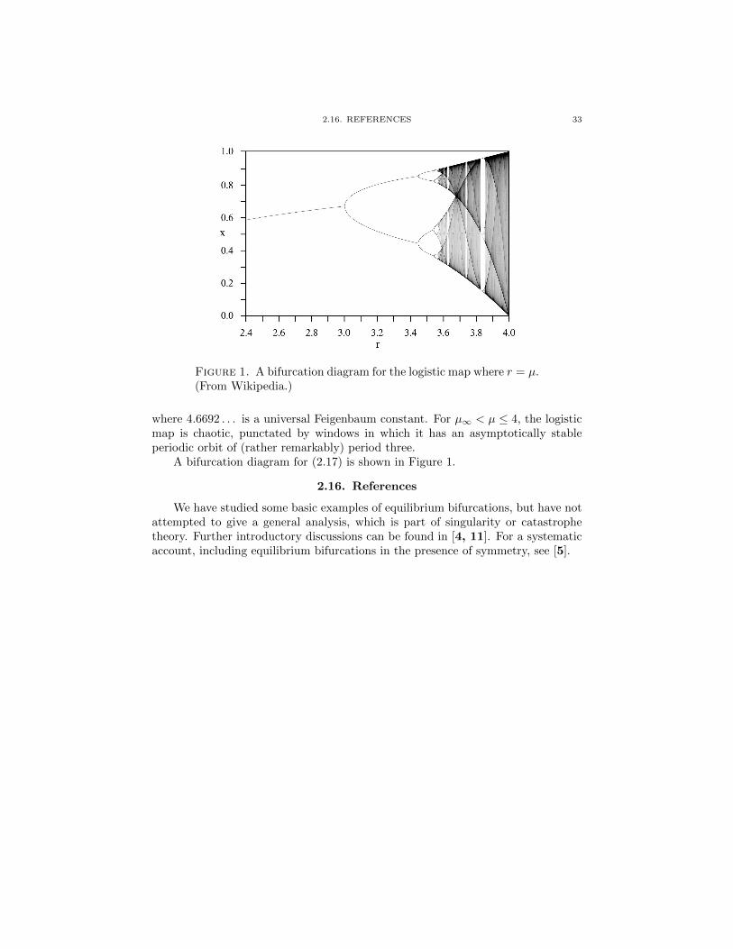
Figure 1. A bifurcation diagram for the logistic map where r = µ.(From Wikipedia.)

where 4.6692 . . . is a universal Feigenbaum constant. For µ∞ < µ ≤ 4, the logisticmap is chaotic, punctated by windows in which it has an asymptotically stableperiodic orbit of (rather remarkably) period three.

A bifurcation diagram for (2.17) is shown in Figure 1.

2.16. References

We have studied some basic examples of equilibrium bifurcations, but have notattempted to give a general analysis, which is part of singularity or catastrophetheory. Further introductory discussions can be found in [4, 11]. For a systematicaccount, including equilibrium bifurcations in the presence of symmetry, see [5].

Bibliography

[1] V. I. Arnold, Ordinary Differential Equations, Spinger-Verlag, 1992.

[2] E. A. Coddington and N. Levinson, Theory of Ordinary Differential Equations, Krieger, 1984.[3] R. Devaney and R. L. Devaney, An Introduction to Chaotic Dynamical Systems, 2nd Ed.,

Westview Press, 2003.

[4] P. Glendinning, Stability, Instability and Chaos, Cambridge University Press, Cambridge,1994.

[5] M. Golubitsky and D. G. Shaeffer, Singularities and Groups in Bifurcation Theory, Vol. 1,

Springer-Verlag, New York, 1985.[6] J. Hale and H. Kocak, Dynamics and Bifurcations, Springer-Verlag, New York, 1991.

[7] J. Guckenheimer and P. Holmes, Nonlinear Oscillations, Dynamical Systems, and Bifurca-tions of Vector Fields, 2nd Ed., Springer-Verlag, 1983.

[8] P. Hartman, Ordinary Differential Equations, 2nd Ed., Birkhauser, 1982.

[9] M. W. Hirsch, S. Smale, and R. L. Devaney, Differential Equations, Dynamical Systems, andan Introduction to Chaos, 2nd Ed., Elsevier, 2004.

[10] S. Strogatz, Nonlinear Dynamics And Chaos, Westview Press, 2001.

[11] S. Wiggins, Introduction to Applied Nonlinear Dynamical Systems and Chaos, Springer-Verlag, New York, 1990.

35

Introduction to Dynamical Systems John K. Hunterhunter/m207/m207.pdf · Introduction to Dynamical...

Documents

Transcript of Introduction to Dynamical Systems John K. Hunterhunter/m207/m207.pdf · Introduction to Dynamical...