Introduction to Computer Vision - Virginia Tech

Object Detection

Computer Vision

Yuliang Zou, Virginia Tech

Many slides from D. Hoiem, J. Hays, J. Johnson, R. Girshick

Administrative stuffs

•HW 4 due 11:59pm on Wed, November 8

•HW 3 grades are out• Average: 116.78, Median: 132.5

• Excellent reports: Pavan Kumar Gundu, Vidur Kakar, TarunKathuria, Prashant Kumar, Snehal More, NareshNagabushan, Sudha Ravali Yellapantula

•Final project proposal• Feedback via emails• Will also set up additional office hours for discussion

Roadmap

Slide from A. Karpathy

Today’s class

•Overview of object category detection

•Traditional methods • Dalal-Triggs detector (basic concept)• Viola-Jones detector (cascades, integral images)

•Deep learning methods• Review of CNN• Two-stage: R-CNN• One-stage: YOLO, SSD, Retina Net

Demo

https://www.youtube.com/watch?time_continue=53&v=VOC3huqHrss

Object Category Detection

•Focus on object search: “Where is it?”

•Build templates that quickly differentiate object patch from background patch

Object or Non-Object?

Dog Model

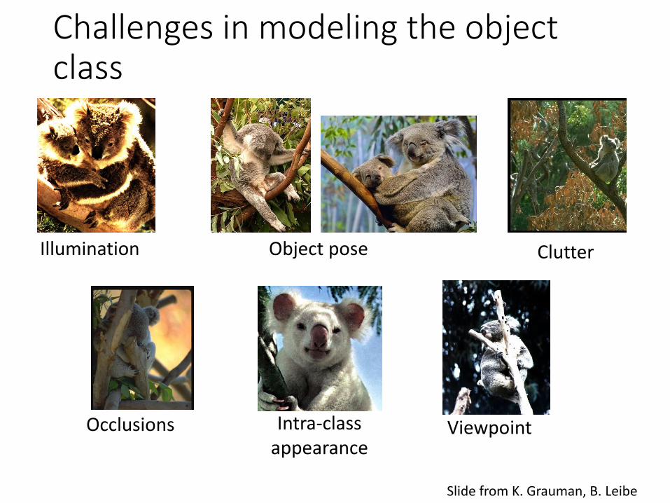
Challenges in modeling the object class

Illumination Object pose Clutter

Intra-class appearance

Occlusions Viewpoint

Slide from K. Grauman, B. Leibe

Challenges in modeling the non-object class

Bad Localization

Confused with Similar Object

Confused with Dissimilar ObjectsMisc. Background

True Detections

General Process of Object Recognition

Specify Object Model

Generate Hypotheses

Score Hypotheses

Resolve Detections

What are the object parameters?

Specifying an object model

1. Statistical Template in Bounding Box• Object is some (x,y,w,h) in image• Features defined wrt bounding box coordinates

Image Template Visualization

Images from Felzenszwalb

Specifying an object model

2. Articulated parts model• Object is configuration of parts• Each part is detectable

Images from Felzenszwalb

Specifying an object model3. Hybrid template/parts model

Detections

Template Visualization

Felzenszwalb et al. 2008



Generate Hypotheses

Score Hypotheses

Resolve Detections

Propose an alignment of the model to the image

Generating hypotheses

1. Sliding window• Test patch at each location and scale


2. Voting from patches/keypoints

Interest PointsMatched Codebook

EntriesProbabilistic

Voting

3D Voting Space(continuous)

x

y

s

ISM model by Leibe et al.


3. Region-based proposal

Endres Hoiem 2010



Generate Hypotheses

Score Hypotheses

Resolve Detections

Mainly-gradient based or CNN features, usually based on summary representation, many classifiers



Generate Hypotheses

Score Hypotheses

Resolve Detections Rescore each proposed object based on whole set

Resolving detection scores1. Non-max suppression

Score = 0.1

Score = 0.8 Score = 0.8

Resolving detection scores2. Context/reasoning

meters

met

ers

Hoiem et al. 2006

Object category detection in computer vision

Goal: detect all pedestrians, cars, monkeys, etc in image

Basic Steps of Category Detection1. Align

• E.g., choose position, scale orientation

• How to make this tractable?

2. Compare• Compute similarity to an

example object or to a summary representation

• Which differences in appearance are important?

Aligned Possible Objects

Exemplar Summary

Sliding window: a simple alignment solution

Each window is separately classified

Statistical Template

•Object model = sum of scores of features at fixed positions

+3 +2 -2 -1 -2.5 = -0.5

+4 +1 +0.5 +3 +0.5 = 10.5

> 7.5?

> 7.5?

Non-object

Object

Example: Dalal-Triggs detector

1. Extract fixed-sized (64x128 pixel) window at each position and scale

2. Compute HOG (histogram of gradient) features within each window

3. Score the window with a linear SVM classifier

4. Perform non-maxima suppression to remove overlapping detections with lower scores

Navneet Dalal and Bill Triggs, Histograms of Oriented Gradients for Human Detection, CVPR05

Slides by Pete Barnum Navneet Dalal and Bill Triggs, Histograms of Oriented Gradients for Human Detection, CVPR05

•Tested with• RGB• LAB• Grayscale

•Gamma Normalization and Compression• Square root• Log

Slightly better performance vs. grayscale

Very slightly better performance vs. no adjustment

uncentered

centered

cubic-corrected

diagonal

Sobel


Outperforms

•Histogram of gradient orientations

• Votes weighted by magnitude• Bilinear interpolation between cells

Orientation: 9 bins (for unsigned angles)

Histograms in 8x8 pixel cells


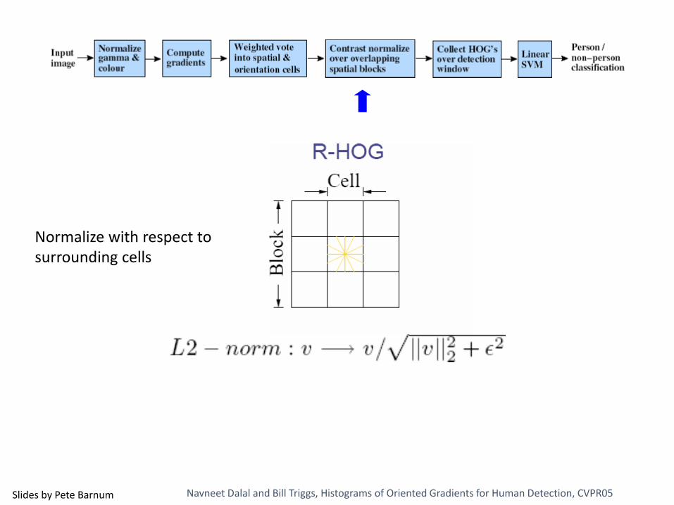
Normalize with respect to surrounding cells


X=


# features = 15 x 7 x 9 x 4 = 3780

# cells

# orientations

# normalizations by neighboring cells


pos w neg w

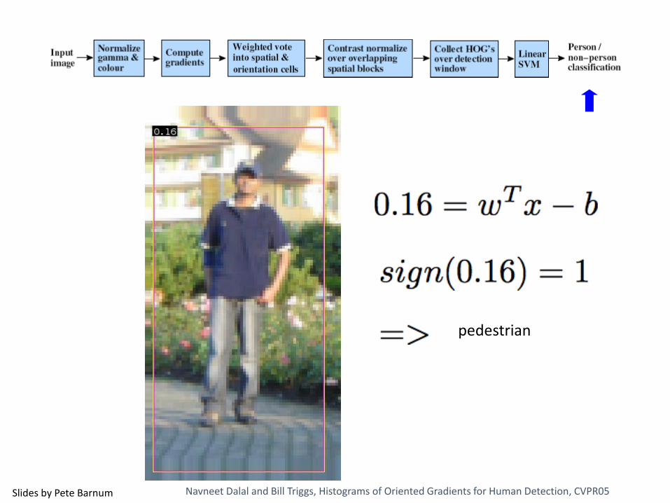
pedestrian


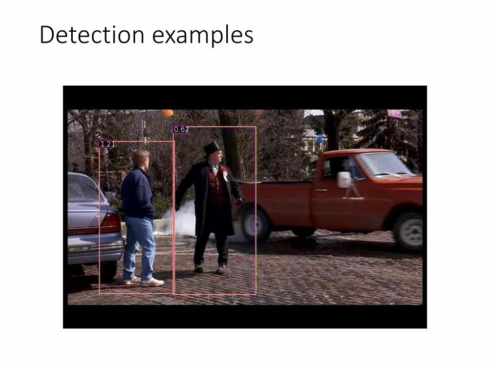
Detection examples

Viola-Jones sliding window detector

Fast detection through two mechanisms

•Quickly eliminate unlikely windows

•Use features that are fast to compute

Viola and Jones. Rapid Object Detection using a Boosted Cascade of Simple Features (2001).

http://www.cs.ubc.ca/~lowe/425/violaJones01.pdf

Cascade for Fast Detection

Examples

Stage 1H1(x) > t1?

Reject

No

Yes

Stage 2H2(x) > t2?

Stage NHN(x) > tN?

Yes

… Pass

Reject

No

Reject

No

• Choose threshold for low false negative rate

• Fast classifiers early in cascade

• Slow classifiers later, but most examples don’t get there

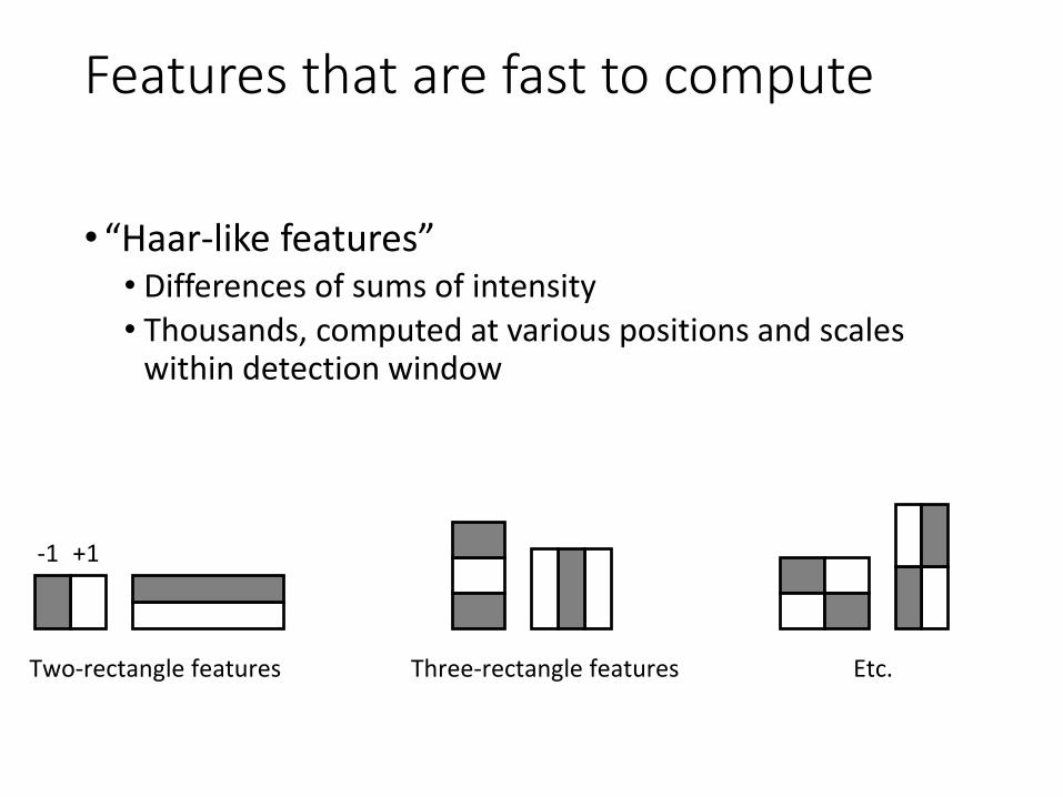
Features that are fast to compute

• “Haar-like features”• Differences of sums of intensity• Thousands, computed at various positions and scales

within detection window

Two-rectangle features Three-rectangle features Etc.

-1 +1

Integral Images

• ii = cumsum(cumsum(im, 1), 2)

x, y

ii(x,y) = Sum of the values in the grey region

How to compute A+D-B-C?

How to compute B-A?

Top 2 selected features

Viola Jones Results

MIT + CMU face dataset

Speed = 15 FPS (in 2001)

Something to think about…

•Sliding window detectors work • very well for faces• fairly well for cars and pedestrians• badly for cats and dogs

•Why are some classes easier than others?

Recap – Convolutional layer

•Convolutional layer1. Local connectivity2. Weight sharing

Local Connectivity

• # input units (neurons): 7

• # hidden units: 3

• Number of parameters• Global connectivity: 3 x 7 = 21

• Local connectivity: 3 x 3 = 9

Input layer

Hidden layer

Global connectivity Local connectivity

Weight Sharing

Input layer

Hidden layer

• # input units (neurons): 7

• # hidden units: 3

• Number of parameters– Without weight sharing: 3 x 3 = 9

– With weight sharing : 3 x 1 = 3

w1

w2

w3

w4

w5

w6

w7

w8

w9

Without weight sharing With weight sharing

w1

w2

w3 w1

w2

w3

w1

w2

w3

How it works?

Credit: Andrej Karpathy

Live demo: http://cs231n.github.io/assets/conv-demo/index.html

http://cs231n.github.io/assets/conv-demo/index.html

Recap – Fully-connected layer

• Each output node is connected to all the input nodes

• Fixed number of input nodes

• Fixed number of output nodes


Recap – Pooling layer

• Reduce the feature size

• Introduce a bit invariance (translation, rotation)


Recap – Activation

• Introduce the non-linearity


Put them all together

• Train the deep convolutional neural net with simple chain-rule (a.k.a back propagation)


Tricks - Dropout

• Randomly set some nodes to zero during training– i.e. Each node will be set to zero with probability p

– Need to rescale the output, divided by (1-p)

• Usually put it after fc layers, to avoid overfitting


Tricks – Batch Normalization

• More robust to bad initialization


Deep learning methods

• Let’s have a 2-min break!

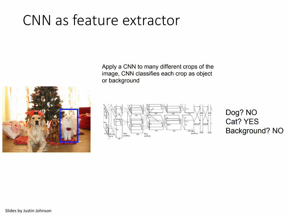
CNN as feature extractor

Image credit: Justin Johnson


Slides by Justin Johnson


•What could be the problems?


•What could be the problems?• Suppose we have a 600 x 600 image, if sliding window size is

20 x 20, then have (600-20+1) x (600-20+1) = ~330,000 windows




• Sometimes we want to have more accurate results -> multi-scale detection• Resize image

• Multi-scale sliding window




• Sometimes we want to have more accurate results -> multi-scale detection• Resize image

• Multi-scale sliding window

• For each image, we need to do the forward pass in the CNN for ~330,000 times. -> Slow!!!

Region Proposal•Solution

• Use some fast algorithms to filter out some regions first, only feed the potential region (region proposals) into CNN

• E.g. selective search

Uijilings et al. IJCV 2013

R-CNN (Girshick et al. CVPR 2014)

• Replace sliding windows with “selective search” region proposals (Uijilings et al. IJCV 2013)• Extract rectangles around regions and resize to 227x227• Extract features with fine-tuned CNN (that was initialized

with network trained on ImageNet before training)• Classify last layer of network features with SVM, refine

bounding box localization (bbox regression) simultaneously

http://arxiv.org/pdf/1311.2524.pdf

http://arxiv.org/pdf/1311.2524.pdf

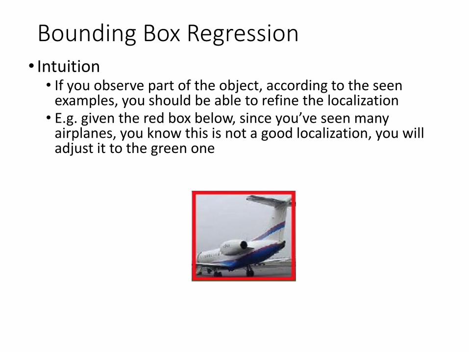
Bounding Box Regression• Intuition

• If you observe part of the object, according to the seen examples, you should be able to refine the localization

• E.g. given the red box below, since you’ve seen many airplanes, you know this is not a good localization, you will adjust it to the green one


•What could be the problems?• Repetitive computation! For overlapping regions, we feed it

multiple times into CNN

Fast R-CNN (Girshick ICCV 2015)

•Solution• Why not feed the whole image into CNN only once! Then

crop features instead of image itself

https://arxiv.org/pdf/1504.08083.pdf


Fast R-CNN (Girshick ICCV 2015)

•How to crop features?• Since we have fully-connected layers, the size of feature map

for each bounding box should be a fixed number



Fast R-CNN (Girshick et al. ICCV 2015)


for each bounding box should be a fixed number• Resize/Interpolate the feature map as fixed size?

• Not optimal. This operation is hard to backprop -> we cannot train the convlayers for this problem





for each bounding box should be a fixed number• Resize/Interpolate the feature map as fixed size?

• Not optimal. This operation is hard to backprop -> we cannot train the convlayers for this problem

• RoI (Region of Interest) Pooling



RoI Pooling

•Step 1: Get bounding box for feature map from bounding box for image• Due the (down)convolution / pooling operations, feature

map would have a smaller size than the original image


Feature map


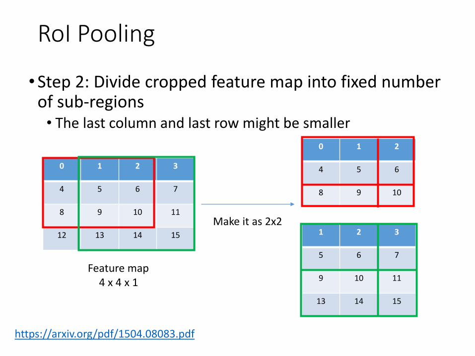
RoI Pooling

•Step 2: Divide cropped feature map into fixed number of sub-regions• The last column and last row might be smaller


0 1 2 3

4 5 6 7

8 9 10 11

12 13 14 15

Feature map4 x 4 x 1

0 1 2

4 5 6

8 9 10

Make it as 2x21 2 3

5 6 7

9 10 11

13 14 15


RoI Pooling

•Step 3: For each sub-region, perform max pooling (pick the max one)


0 1 2

4 5 6

8 9 10Max pooling

5 6

9 10



•What could be the problems?• Why we need the region proposal pre-processing step?

That’s not “deep learning” at all. Not cool!

Uijilings et al. IJCV 2013

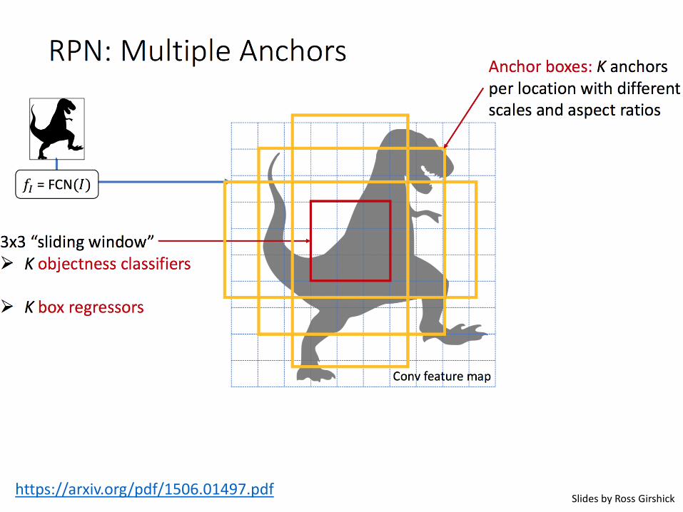
Faster R-CNN (Ren et al. NIPS 2015)

•Solution• Why not generate region proposals using CNN??! -> RPN

https://arxiv.org/pdf/1506.01497.pdf Image credit:http://zh.gluon.ai/chapter_computer-vision/object-detection.html


http://zh.gluon.ai/chapter_computer-vision/object-detection.html


https://arxiv.org/pdf/1506.01497.pdfSlides by Ross Girshick



•Solution• Why not generate region proposals using CNN??!

https://arxiv.org/pdf/1506.01497.pdfSlides by Ross Girshick



•What could be the problems




•What could be the problems• Two-stage detection pipeline is still too slow to apply on

real-time videos



One-stage detection

•Solution• Don’t generate object proposals!• Consider a tiny subset of the output space by design; directly

classify this small set of boxes

Image credit:http://zh.gluon.ai/chapter_computer-vision/object-detection.html

http://zh.gluon.ai/chapter_computer-vision/object-detection.html

One-stage detection

•Solution• Don’t generate object proposals!

Slides by Justin Johnson

One-stage detection


One-stage detection

•What could be the problems?• The extreme foreground-background class imbalance -> we

have a lot more negative examples.

One-stage detection

•What could be the problems?• The extreme foreground-background class imbalance -> we

have a lot more negative examples. • Even though they have small loss values, the gradients

overwhelm the model

Focal Loss for Dense Object Detection (Lin et al. ICCV 2017)

•Solution• For easy examples, we down-weight it loss, so that the

gradients from these example have smaller impact to the model



One-stage detection

Mistakes are often reasonableBicycle: AP = 0.73

Confident Mistakes

R-CNN results

Horse: AP = 0.69 Confident Mistakes

Mistakes are often reasonable

R-CNN results

Influential Works in Detection• Sung-Poggio (1994, 1998) : ~2100 citations

• Basic idea of statistical template detection (I think), bootstrapping to get “face-like” negative examples, multiple whole-face prototypes (in 1994)

• Rowley-Baluja-Kanade (1996-1998) : ~4200• “Parts” at fixed position, non-maxima suppression, simple cascade, rotation,

pretty good accuracy, fast

• Schneiderman-Kanade (1998-2000,2004) : ~2250• Careful feature/classifier engineering, excellent results, cascade

• Viola-Jones (2001, 2004) : ~20,000• Haar-like features, Adaboost as feature selection, hyper-cascade, very fast, easy

to implement

• Dalal-Triggs (2005) : ~11000• Careful feature engineering, excellent results, HOG feature, online code

• Felzenszwalb-Huttenlocher (2000): ~1600• Efficient way to solve part-based detectors

• Felzenszwalb-McAllester-Ramanan (2008,2010)? ~4000• Excellent template/parts-based blend

Influential Works in Detection

Fails in commercial face detection

•Things iPhoto thinks are faces

http://www.oddee.com/item_98248.aspx

http://www.flickr.com/groups/977532@N24/pool/

http://www.oddee.com/item_98248.aspx

Summary: statistical templates

Propose Window

Sliding window: scan image pyramid

Region proposals: edge/region-based, resize to fixed window

Extract Features

HOG

CNN features

Fast randomized features

Classify

SVM

Boosted stubs

Neural network

Post-process

Non-max suppression

Segment or refine localization

Next class

• Image Segmentation

https://people.eecs.berkeley.edu/~jonlong/long_shelhamer_fcn.pdf

https://people.eecs.berkeley.edu/~jonlong/long_shelhamer_fcn.pdf

Introduction to Computer Vision - Virginia Tech

Documents

Transcript of Introduction to Computer Vision - Virginia Tech