Introduction to combinatorics1 - Technion · A large part of combinatorics is counting and...

Introduction to combinatorics1

A course instructed by Amir Yehudayoff, Department of Mathematics, Technion-IIT

1An apology: this text probably contains errors.

Contents

1 Preface 5

2 Preliminaries 7

3 Counting 9

3.1 Basic methods . . . . . . . . . . . . . . . . . . . . . . . . . . . . . . . . . 9

3.2 Choosing . . . . . . . . . . . . . . . . . . . . . . . . . . . . . . . . . . . . 10

3.3 Binomial coefficients . . . . . . . . . . . . . . . . . . . . . . . . . . . . . 12

3.4 Catalan numbers . . . . . . . . . . . . . . . . . . . . . . . . . . . . . . . 16

3.5 Inclusion-exclusion . . . . . . . . . . . . . . . . . . . . . . . . . . . . . . 18

3.6 Fibonacci numbers . . . . . . . . . . . . . . . . . . . . . . . . . . . . . . 20

3.7 Linear recurrences . . . . . . . . . . . . . . . . . . . . . . . . . . . . . . . 22

3.8 Generating functions . . . . . . . . . . . . . . . . . . . . . . . . . . . . . 24

4 Existential proofs: the pigeonhole principle 29

5 Graphs 33

5.1 Basic notions . . . . . . . . . . . . . . . . . . . . . . . . . . . . . . . . . 33

5.2 Trees . . . . . . . . . . . . . . . . . . . . . . . . . . . . . . . . . . . . . . 36

5.3 Bipartite graphs . . . . . . . . . . . . . . . . . . . . . . . . . . . . . . . . 37

5.4 Planarity . . . . . . . . . . . . . . . . . . . . . . . . . . . . . . . . . . . . 38

5.5 Colorings . . . . . . . . . . . . . . . . . . . . . . . . . . . . . . . . . . . 41

5.6 Ramsey numbers . . . . . . . . . . . . . . . . . . . . . . . . . . . . . . . 43

5.7 Matchings . . . . . . . . . . . . . . . . . . . . . . . . . . . . . . . . . . . 46

6 Stable marriages 51

3

4 CONTENTS

Chapter 1

Preface

These notes summarize an introductory course to combinatorics. Part of the goals of this

course is to learn the language of mathematics, get familiar with notions and basic ideas,

and improving the ability to understand and investigate abstract concepts. Remember

to ask as many questions as you wish, but try to think about it a little before asking.

5

6 CHAPTER 1. PREFACE

Chapter 2

Preliminaries

We begin with a short recollection of notions and notation.

Sets

A = {1, 2, 3}, a ∈ A, A ⊆ B.

∅,N = {1, 2, 3, . . . , },Z = {. . . ,−2,−1, 0, 1, . . .}, [n] = {1, 2, . . . , n}.A ∩B,A ∪B,A \B, and Venn diagrams.

A×B = {(a, b) : a ∈ A, b ∈ B}.

If you see notation that you do not understand, ask.

Induction

Induction is a framework to prove theorems, mostly on properties of N. It is used to

prove theorem of the form “for every n ∈ N, we have n ∈ P” where P is some “property”

of integers.

Proofs by induction have two parts: 1. “Base” in which a few preliminary cases are

verified (proving that say 1, 2 ∈ P ). 2. “Step” in which we prove that for all n ≥ 2 if

n ∈ P then n+ 1 ∈ P .

The axiom underlying proofs by induction is: for every non-empty subset of the

integers has a minimum element.

Here is an example.

Claim 1. For every n ∈ N,n∑i=1

i =n(n+ 1)

2.

7

8 CHAPTER 2. PRELIMINARIES

Proof. Base: Since 1 = 1 · 2/2, the claim holds for n = 1. Step: Assume the claim holds

for n:n∑i=1

i =n(n+ 1)

2.

Thus,n+1∑i=1

i = n+ 1 +n∑i=1

i = n+ 1 +n(n+ 1)

2=

(n+ 1)(n+ 2)

2.

More abstractly, proofs by induction are useful when we wish to prove a statement

on a collection of objects, where each object can be constructed using a finite list of

“composition steps” from a finite list of “basic objects”. In the case of N, every natural

number satisfied n = (n− 1) + 1, so it can be constructed using the operation +1 from

1.

When using induction, we need to pay attention to the rules of the game. For example

(Polya): All walls have the same color. “Proof”: Base: this wall is white. Step: If we

have n walls numbered {1, 2, . . . , n} then the set {1, 2, . . . , n− 1} of walls has the same

color and the set {2, . . . , n} has the same color. Therefore, all walls in {1, 2, . . . , n} have

the same color. � What is mistake?

Comparing sizes

We shall use the following simple facts. Let A,B be finite sets.

• If there is a one-to-one map from A to B then |A| ≤ |B|.

• If there is a map from A onto B then |A| ≥ |B|.

• If there is a one-to-one and onto map from A to B then |A| = |B|.

Chapter 3

Counting

A large part of combinatorics is counting and enumeration; calculating or estimating

the size of a given set of objects, like in how many possible outcomes to the lottery are

there, or in how many ways can we pair students in a given class. In this chapter, we

shall see a few basic tools for answering such questions, mostly by considering examples.

3.1 Basic methods

Cartesian products

If A,B are finite sets then

|A×B| = |A| · |B|.

More generally, by induction,

|A1 × A2 . . .× An| =n∏i=1

|Ai|.

Bijections

What is the number of subsets of [n]? In other words, what is the size of {S : S ⊆ [n]}?2n.

Indeed, denote by P the number of subsets of [n]. For every S ∈ P , define x(S) ∈{0, 1}n by (x(S))i = 1 iff i ∈ S. The vector x(S) is called the indicator of S. The map

S 7→ x(S) is a one-to-one and onto map from P to {0, 1}n. The size of {0, 1}n is

|{0, 1}n| = |{0, 1}|n = 2n.

9

10 CHAPTER 3. COUNTING

Double counting

Problem 2. In a classroom there are 32 boys, each boy knows 5 girls, and each girl

knows 8 boys (“knowing” is symmetric). How many girls in class are there?

Solution. Denote by A the set of boys, and by B the set of girls. For a ∈ A and b ∈ B,

let f(a, b) = 1 if a knows b, and f(a, b) = 0 otherwise. Thus,∑a∈A

∑b∈B

f(a, b) =∑a∈A

5 = 5|A| = 5 · 32.

On the other hand, the sum is also equals to∑b∈B

∑a∈A

f(a, b) = 8|B|.

So,

|B| = 5 · 4 = 20.

Permutations

A permutation of [k] is a one-to-one and onto map from [k] to [k]. It is a re-ordering of

k. Denote by Π = Πk the permutation on [k]. How many permutation of k are there?

We need to decide what is π(1). There are k options. Then we need to decide what is

π(2). There are now k − 1 options. And so forth. Overall,

|Π| = k(k − 1)(k − 2) . . . 1 = k!.

3.2 Choosing

Assume that there are n numbered balls and we want to choose k of them. There are

four options:

no repetition repetition allowed

order matters ordered sets of size k (2) sequences of length k (1)

order does not matter sets of size k (3) multi-sets of size k (4)

3.2. CHOOSING 11

1. Sequences of length k

We are interested in the size of

T1 = {(i1, i2, . . . , ik) ∈ [n]k} = [n]k,

which is nk.

2. Ordered sets of size k


T2 = {(i1, i2, . . . , ik) ∈ [n]k : ∀j 6= j′ ij 6= ij′}.

How many options for i1? n.

After fixing i1, how many options for i2? n− 1.

After fixing i1, i2, how many options for i3? n− 2.

Overall, the size of this set is

|T2| = n(n− 1)(n− 2) · · · (n− k + 1) =n!

(n− k)!.

3. Sets of size k


T3 = {{i1, i2, . . . , ik} ⊆ [n]} = {S ⊆ [n] : |S| = k} :=

([n]

k

).

Now, fix I = {i1 < i2 < . . . < ik} ∈ T3. For every permutation π of [k], there is a

sequence (iπ(1), iπ(2), . . . , iπ(k)) ∈ T2.The map

T3 × Πk → T2

(I, π) 7→ (iπ(1), iπ(2), . . . , iπ(k))

is one-to-one and onto (verify). Thus,

|T3 × Πk| = |T2|

and

|T3| =|T2||Πk|

=n!

(n− k)!k!:=

(n

k

).


4. Multi-sets of size k

We are interested in the number of ways to choose k balls from n when order does not

matter and repetitions are allowed. Such a choice is given by

x = (x1, x2, . . . , xn)

where each xi ≥ 0, and∑n

i=1 xi = k. The number xi encodes the number of times i

appears in the choice.

We think of x as follows. Image n boxes in a row and k bottles, where box i contains

exactly xi bottles. We can think of bottles as B’s and of separator between boxes as |.For example, for n = 5 and (1, 0, 0, 2, 1) with k = 4 we get

B|||BB|B.

In the left box there is 1 bottle, in the one to its right there are 0 bottles and so forth.

So every such x corresponds to a sequence of length n− 1 +k symbols, k of which are B

and n− 1 are |. What is the number of such sequences? We just need to choose where

to put the B’s, so

|T4| =(n− 1 + k

k

).

3.3 Binomial coefficients

We now investigate one of the most common number in mathematics: The number of

sets of size k in [n]. We saw ∣∣∣∣([n]

k

)∣∣∣∣ =

(n

k

).

For notational convenience, if k < 0 or k > 0 we set(nk

)= 0; and

(00

)= 1. These are

called the binomial coefficients, and are read “n choose k”.

Inductive formula

Claim 3. For every n ≥ 2 and 0 ≤ k ≤ n, we have(n

k

)=

(n− 1

k

)+

(n− 1

k − 1

).

Proof. Can be proved by direct calculation.

Here is a more explanatory proof. If S ⊆ [n] is of size |S| = k, then there are two

options: n ∈ S and n 6∈ S. If n ∈ S then S ∩ [n− 1] is a subset of [n− 1] of size k − 1,

3.3. BINOMIAL COEFFICIENTS 13

and if n 6∈ S then S ∩ [n− 1] is a subset of [n− 1] of size k. That is, there is a bijection

between([n]k

)and the disjoint union of

([n−1]k

)and

([n−1]k−1

).

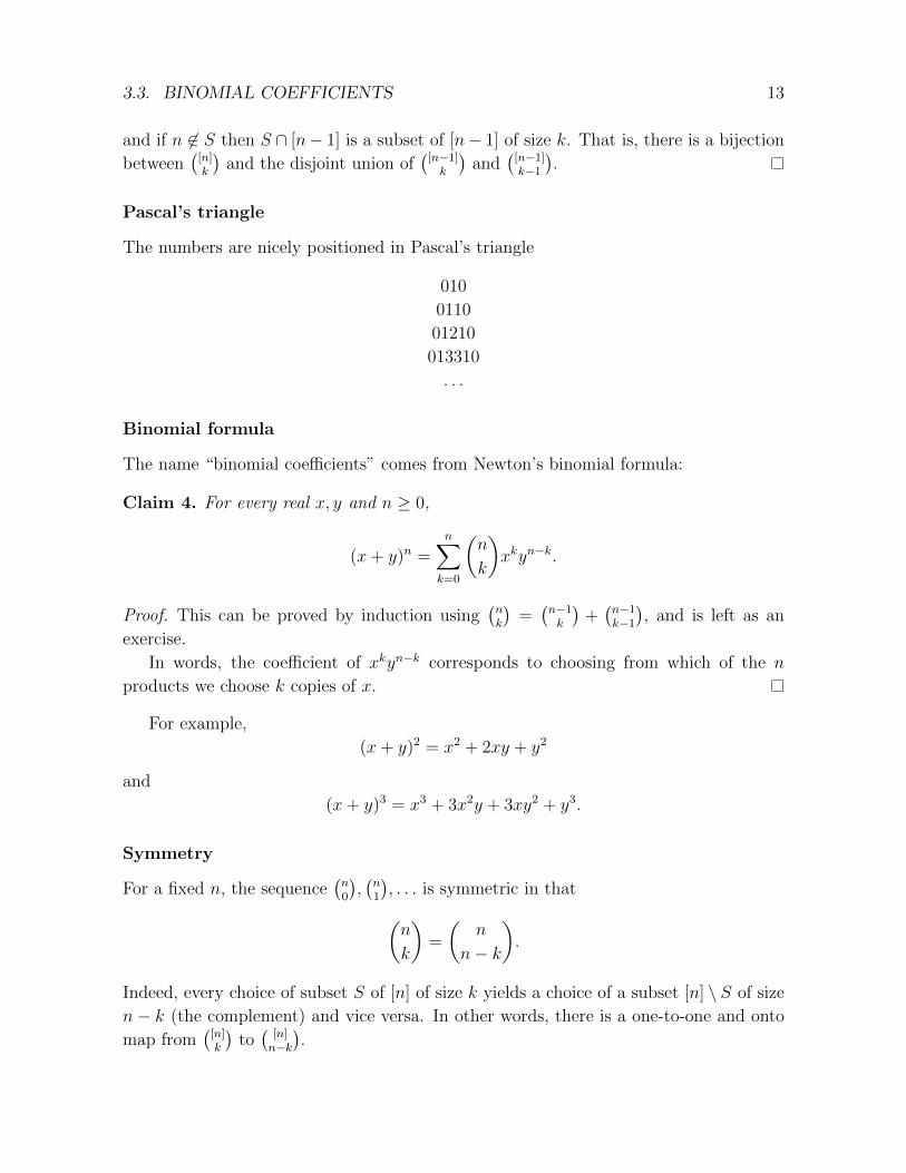
Pascal’s triangle

The numbers are nicely positioned in Pascal’s triangle

010

0110

01210

013310

. . .

Binomial formula

The name “binomial coefficients” comes from Newton’s binomial formula:

Claim 4. For every real x, y and n ≥ 0,

(x+ y)n =n∑k=0

(n

k

)xkyn−k.

Proof. This can be proved by induction using(nk

)=(n−1k

)+(n−1k−1

), and is left as an

exercise.

In words, the coefficient of xkyn−k corresponds to choosing from which of the n

products we choose k copies of x.

For example,

(x+ y)2 = x2 + 2xy + y2

and

(x+ y)3 = x3 + 3x2y + 3xy2 + y3.

Symmetry

For a fixed n, the sequence(n0

),(n1

), . . . is symmetric in that(n

k

)=

(n

n− k

).

Indeed, every choice of subset S of [n] of size k yields a choice of a subset [n] \ S of size

n− k (the complement) and vice versa. In other words, there is a one-to-one and onto

map from([n]k

)to(

[n]n−k

).


Unimodality

For a fixed n, the sequence(n0

),(n1

), . . . is unimodal, that is, it increases and then de-

creases.

Claim 5.(nk+1

)≥(nk

)if and only if 2k ≤ n− 1.

Roughly speaking, the sequence grows until the middle and then starts to decrease.

Symmetry implies that if it grows to the middle then it must decay after the middle.

The maximum is attained at k = bn/2c.

Proof. (nk+1

)(nk

) =n!

(k + 1)!(n− k − 1)!· k!(n− k)!

n!=n− kk + 1

.

Identities

We shall see several identities and prove them in various ways.

Claim 6.∑n

k=0

(nk

)= 2n.

Binomial formula.

2n = (1 + 1)n =n∑k=0

(n

k

)1k1n−k =

n∑k=0

(n

k

).

Combinatorial story. The number∑n

k=0

(nk

)is the total number of subsets of [n], which

is 2n.

Claim 7.∑n

k=0 k(nk

)= n2n−1.

Computation. Notice

k

(n

k

)= k

n!

k!(n− k)!= n

(n− 1)!

(k − 1)!(n− k)!= n

(n− 1

k − 1

).

Thus,n∑k=0

k

(n

k

)=

n∑k=0

n

(n− 1

k − 1

)= n2n−1

(need to make sure that k = 0 is also correct).

3.3. BINOMIAL COEFFICIENTS 15

Analytic. By the binomial formula,

f(x) = (1 + x)n =n∑k=0

(n

k

)xk.

Differentiate

f ′(x) = n(1 + x)n−1 =n∑k=0

k

(n

k

)xk−1.

Substitute x = 1.

Combinatorial story. The number∑n

k=0 k(nk

)is the number of choices in: choose a group

inside [n] and then choose a leader for the group. We can first choose the leader and

then choose the rest of the group inside a set of size n− 1.

Claim 8. For n > 0, we have∑n

k=0(−1)k(nk

)= 0.

Proof. Expand 0n = (1− 1)n according to binomial identity.

The claim can be interpreted as follows:

∑even k

(n

k

)=∑odd k

(n

k

).

In other words, the number of subsets of even size is equal to the number of subsets

of odd size in [n]. For example, for n = 4, we have 1 + 6 + 1 = 4 + 4. Try to find a

one-to-one and onto map between the sets of even size to the sets of odd size.

Another way to write the claim is as follows.

Claim 9. Let A be a finite non-empty set. Then,∑S⊆A

(−1)|S| = 0.

Estimations

Although(nk

)is relatively simple to calculate, we sometimes need an estimate which is

even easier to understand (this is a common theme in mathematics).

Theorem 10. (n/k)k ≤(nk

)≤ (ne/k)k for 0 < k ≤ n.


Proof. (n

k

)· (k/n)k ≤

n∑`=0

(n

`

)(k/n)` (all terms are positive)

= (1 + (k/n))n

≤ ek. (1 + x ≤ ex for all x)

If k � n, we can usually think of(nk

)as nk. If k ≈ n, we can think of

(nk

)as cn for

some c > 1.

Theorem 11.(2nn

)≥ 2n/(n+ 1).

Proof. Unimodality implies(2nk

)≤(2nn

). Thus,

2n =2n∑k=0

(2n

k

)≤ (n+ 1)

(2n

n

).

In fact,(2nn

)is, up to constants, equal to 22n/

√n. This can be proved using Stirling’s

formula (n! ≈√n(n/e)n).

3.4 Catalan numbers

Assume that we have n brackets. In how many ways can we legally1 position them?

Examples: for n equals

1. we have 1 option: ().

2. we have 2 options: ()(), (()).

3. we have 5 options: ()()(), (())(), (()()), ((())), ()(()).

4. we have 14 options.



1A legal positioning of brackets is of the form (()(()).

3.4. CATALAN NUMBERS 17

Perhaps the simplest way to understand them is write a recursive formula. The

observation is that the first bracket is closed somewhere E = (E1)E2 where E1, E2 are

legal positioning of brackets with E1 have k brackets and E2 having n− k− 1. So, if we

denote by C(n) the number we are interested in then

C(0) = C(1) = 1

and for n > 1 we have

C(n) =n−1∑k=0

C(k)C(n− 1− k).

For example,

C(2) = C(0)C(1) + C(1)C(0) = 2

and

C(3) = C(0)C(2) + C(1)C(1) + C(2)C(0) = 2 + 1 + 2 = 5.

We can thus calculate C(n) exactly, but this may take a lot of time.

We now find a “formula” for C(n). The basic idea is to “encode” a legal positioning

of brackets as a walk on a grid with certain properties, and then count the number of

walks.

We consider walks on the lattice of points in the plane of the form (x, y) where x, y

are integers and x+ y is even. Draw it.

Our walks will always start at (0, 0), and in each time step t ≥ 0 we move from

(xt, yt) to one of two positions (xt + 1, yt + 1) or (xt + 1, yt − 1). Draw the two options.

We interpret a sequence of brackets: ( means +1 and ) means −1. For example (())

gives (0, 0), (1, 1), (2, 2), (3, 1), (4, 0).

A legal sequence of n brackets gives a walk from (0, 0) to (2n, 0) that stays above

the line y = 0, and vice versa. So C(n) is the number of such walks.

It is in fact easier to calculate a different quantity first. Denote by W = W (n) the

total number of walks from (0, 0) to (2n, 0). (Thus, C(n) < W (n).) Every such walk

has n times with a “+1 step” and n times with a “−1 step”, so

W (n) =

(2n

n

).

Denote by C̄(n) the number of walks that are not of “Catalan” form; walks z =

((x0, y0), . . . , (x2n, y2n)) with y2n = 0 that hit the line y = −1. That is, there exists t ≥ 0

so that yt = −1. Thus,

C(n) = W (n)− C̄(n).

We first compute C̄(n). Given a walk z = ((x0, y0), . . . , (x2n, y2n)) that contributes


to C̄(n), let

T (z) = min{t ≥ 1 : yt = −1};

the first time the walk hits the line y = −1. Thus, T (z) < 2n.

For such z, define R(z) as the walk obtained from z by reflection after time t(z)

with respect to the line y = −1. Draw an example. That is, for t ≤ T (z) we have

(R(z))t = zt and for t > T (z) we have (R(z))t = (t,−yt − 2). Thus, for all such z, we

have (R(z))2n = (2n,−2).

We claim that the map z 7→ R(z) is one-to-one and onto the set of walks from (0, 0)

to (2n,−2). Indeed, this holds since the map R is invertible (it is its own inverse) and

since every walk from (0, 0) to (2n,−2) crosses the line y = −1 at least once.

To compute the number of walk from (0, 0) to (2n,−2), notice that every such walk

has n − 1 times with a “+1 step” and n + 1 times with a “−1 step”. The number of

such walks is therefore

C̄(n) =

(2n

n+ 1

)=

(2n

n− 1

).

Finally,

C(n) =

(2n

n

)−(

2n

n+ 1

)=

(2n)!

n!n!− (2n)!

(n+ 1)!(n− 1)!=

(2n)!

n!n!

(1− n

n+ 1

)=

1

n+ 1

(2n

n

).

As an exercise, you can verify that it satisfies the recursion we saw before. We may

conclude that

C(n) ≈ 22n/n3/2.

Exercise 12. Prove that C(n) is equal to the number of triangulations of a convex

(n+ 2)-gon in the plane.

Examples: C(1) corresponds to the triangle, C(2) corresponds to the 2 triangulations

of a square, etc.

3.5 Inclusion-exclusion

Assume that we have n finite sets A1, . . . , An, and we know their sizes. What can we

say about the size of their union⋃ni=1Ai?

Theorem 13. |⋃ni=1Ai| ≤

∑ni=1 |Ai|.

Proof. Let

A =⋃i

Ai.

3.5. INCLUSION-EXCLUSION 19

For a ∈ A, let

Ia = {i ∈ [n] : a ∈ Ai}.

Thus, |Ia| ≥ 1 for all a ∈ A. So,

|A| =∑a∈A

1 ≤∑a∈A

|Ia| =∑a∈A

n∑i=1

1a∈Ai=

n∑i=1

∑a∈A

1a∈Ai=

n∑i=1

|Ai|.

This inequality is far from being tight, for example if A1 = A2 = · · · = An. So, if we

have more data we can say more accurate things. If for example we know the sizes of

the pairwise intersections then we can bound:

Theorem 14. |⋃ni=1Ai| ≥

∑ni=1 |Ai| −

∑1≤i<j≤n |Ai ∩ Aj|.

Left as exercise.

If we have information on all intersection sizes, we can compute the size exactly.

Example: If X, Y, Z are finite sets then

|X ∪ Y ∪ Z| = |X|+ |Y |+ |Z| − |X ∩ Y | − |X ∩ Z| − |Y ∩ Z|+ |X ∩ Y ∩ Z|.

Draw a Venn diagram. In general:

Theorem 15 (Inclusion-exclusion).∣∣∣∣∣n⋃i=1

Ai

∣∣∣∣∣ =∑

1≤i≤n

|Ai| −∑

1≤i<j≤n

|Ai ∩ Aj|+

+∑

1≤i<j<k≤n

|Ai ∩ Aj ∩ Ak|+ . . .+ (−1)n+1|A1 ∩ A2 ∩ · · · ∩ An|

=∑

S⊆[n]:S 6=∅

(−1)|S|+1

∣∣∣∣∣⋂i∈S

Ai

∣∣∣∣∣ .Proof. Recall that for every finite non-empty B, we have

∑S⊆B(−1)|S| = 0 so we have

a complicated way to write one:

1 =∑

S⊆B:S 6=∅

(−1)|S|+1.

Let

A =n⋃i=1

Ai.


For a ∈ A, let

Ia = {i ∈ [n] : a ∈ Ai}.

For every a ∈ A and non-empty S ⊆ [n], we have that S ⊆ Ia if and only if a ∈⋂i∈S Ai.

Therefore,

|A| =∑a∈A

1

=∑a∈A

∑S⊆Ia:S 6=∅

(−1)|S|+1

=∑

S⊆[n]:S 6=∅

(−1)|S|+1∑

a∈A:S⊆Ia

1

=∑

S⊆[n]:S 6=∅

(−1)|S|+1

∣∣∣∣∣⋂i∈S

Ai

∣∣∣∣∣ .

3.6 Fibonacci numbers

Leonardo Pisano Bigollo studied the population size of rabbits in the 12th century in

Pisa (as his name suggests). His name later became Fibonacci (some explanation to

name change: “filius Bonacci” used in the title of his book which means “the son of

Bonaccio”). He came up with the following sequence: Think of F (n) the population

size in generation n. Assume that there is one female rabbit at time 1, that rabbits live

forever, and that at each month from the second month it is born, every female produces

one extra female. How many female rabbits are there after n months?

That is, what is F (n) the is defined as follows? F (1) = 1, F (2) = 1, F (3) = 2, and

in general for n > 1, all the rabbits from time n− 1 are alive at time n, and all rabbits

from time n− 2 reproduce, so

F (n) = F (n− 1) + F (n− 2).

We have a recursive formula for F (n), but can we find a formula that gives more

information about F (n)? The answer is yes, and we will use simple linear algebra to do

so.

For n ≥ 0, define a two-dimensional vector

vn = (F (n), F (n+ 1)).

3.6. FIBONACCI NUMBERS 21

So v0 = (0, 1), v1 = (1, 1) and so forth (we set F (0) = 0). The first observation is that

the recursive definition of F (n) implies that

vn+1 = Avn

where

A =

[0 1

1 1

].

In particular, we get the following simple formula:

vn = Anv0.

But what is An? To understand An better, we diagonalize A. Write

A = U−1DU,

where

U =

[ √5−12

1−√5−12

1

]is orthogonal UUT = I and

D =

[1+√5

20

0 1−√5

2

]is diagonal. We will not explain how to find U,D for now. But how is this helpful? Well,

An = (UDU−1)(UDU−1) · · · (UDU−1) = UDnU−1 = U

(1+√5

2

)n0

0(

1−√5

2

)nU−1.

Since vn = Anv0, we conclude that there are two real numbers a, b so that for all n,

F (n) = a

(1 +√

5

2

)n

+ b

(1−√

5

2

)n

.

We can find a, b using F (0) = 0 and F (1) = 1. These two equalities imply a = −b and

1 = a

(1 +√

5

2

)− a

(1−√

5

2

)or

a =1√5.


Finally, for all n,

F (n) =1√5

(1 +√

5

2

)n

− 1√5

(1−√

5

2

)n

.

It may be surprising that the r.h.s. above is even integer. It also tells us that for

large n, the value of F (n) is close to 1√5

(1+√5

2

)n.

The golden ratio

The number φ = 1+√5

2is called the golden ratio. It is one of the solutions to the

equation x2− x− 1 = 0, or x = 1/(x− 1). A 1×φ rectangles thus have some symmetry

(draw). Another equation is x = 1 + 1/x, which shows that as infinite fraction (“shever

meshulav”) it is equal to

φ = 1 +1

1 + 11+ 1

...

.

The sequence8

5,13

8,21

13, . . .

converges to φ.

This is related to that the Fibonacci sequence appears in many spirals in nature,

like in pine cones where the number of spirals of “opposite” type are two consecutive

numbers in sequence.

3.7 Linear recurrences

The Fibonacci sequence is just one example of a more general phenomenon.

Definition 16. A sequence F (1), F (2), . . . is a (homogenous) linear recurrence of order

r if for every n > r we have

F (n) = a1F (n− 1) + a2F (n− 2) + . . .+ arF (n− r)

where a1, . . . , ar are some constants.

The Fibonacci sequence is of order two. Given a1, . . . , ar, to specify F we need to

choose F (1), . . . , F (r).

The collection of sequences satisfying the rule is a vector space of dimension r. The

collection of Fibonacci sequences is a vector space of dimension two.

We now explain how to find a formula for the general term of such a sequence. We

can use linear algebra, as we did for the Fibonacci sequence, but here we use a seemingly

3.7. LINEAR RECURRENCES 23

different approach (which is actually equivalent). We start by searching for sequences

of the form

F (n) = xn

for some x ∈ R. This gives for every n > r the equation

xn = a1xn−1 + a2x

n−2 + . . .+ arxn−r.

The value x = 0 is always a solution, and if x 6= 0 this is equivalent to

p(x) = xr − a1xr−1 − a2xr−2 − . . .− ar = 0,

which is a polynomial equation of degree r.

Definition 17. The polynomial p(x) is the characteristic polynomial of the recurrence

formula.

For Fibonacci,

p(x) = x2 − x− 1.

For now, let us assume that this equation has r different real solutions (there are

always at most r solutions, but sometimes less than r, and sometimes some roots are

the same). For Fibonacci the 2 roots are

x1 =1 +√

5

2, x2 =

1−√

5

2.

So the r sequences

(xn1 ), (xn2 ), . . . , (xnr )

satisfy the recurrence formula. In fact, they form a basis to the space of sequences.

Specifically, we can write every F as

F (n) = α1xn1 + α2x

n2 + . . .+ αrx

nr .

How do we find α = (α1, . . . , αr)? Using the initial conditions: We have r equations

F (i) = α1xi1 + α2x

i2 + . . .+ αrx

ir

for 1 ≤ i ≤ r, and we have r variable, α.

For Fibonacci,

0 = F (0) = α1x01 + α2x

02, 1 = F (1) = α1x

11 + α2x

12,


which yields

α1 =1√5, α2 = −α1.

In general, there is always a solution if the r roots are different. This is a theorem

from linear algebra, which we shall not prove.2

Let us summarize.

1. We are given a recurrence formula of order r, as above. That is, we are given

a1, . . . , ar and F (1), . . . , F (r).

2. This defines the characteristic polynomial p(x), which has degree r.

3. We try to find all root of p.

4. If p has r different roots, then the formula of a generic term in sequence is of the

form F (n) =∑r

i=1 αixni .

5. To find α, we need to solve r equations in r variables.

Comments:

1. You will see examples in the exercise.

2. Similar to differential equations.

We did not cover:

What if not all roots are distinct? What if the formula is not homogenous? ...

3.8 Generating functions

Generating functions is a way to use abstract algebra to solve combinatorial problems

(there are applications in other areas as well).

First, the definition:

2Why? We can write it in matrix form:f = Xα

where f = (F (1), . . . , F (r)), and Xi,j = Xij is r × r. If all roots are equal there is a unique solution.

Theorem 18. If x1, . . . , xr are r distinct numbers, then the matrix X is invertible.

Hint. det(X) 6= 0.

3.8. GENERATING FUNCTIONS 25

Definition 19. A generating function f is of the form

f =∞∑n=0

fnxn.

It is a formal infinite sum.

Arithmetic

We can sum and multiply two functions f, g. The rules are:

(f + g)n = fn + gn

and

(f · g)n =n∑k=0

fkgn−k.

These operations are commutative.

Examples:

The function 0 := 0 + 0 · x+ 0 · x2 + . . . is so that f + 0 = f for all f , and the function

1 := 1 + 0 · x+ 0 · x2 + . . . is so that 1 · f = f for all f .

Comment:

We do not care for now if f actually defines a function, but think of it abstractly.

One more example:

The function f =∑∞

n=0 xn, or fn = 1 for all n. We claim that the function g = 1 − x,

for which g0 = 1, g1 = −1 and gn = 0 for n > 1, is the inverse of f . That is, g · f = 1.

Indeed, for n > 1,

(g · f)n =n∑k=0

gkfn−k = fn − fn−1 = 0

and

(g · f)0 = g0f0 = 1.

We write it as

(1− x)f = 0

or

f =1

1− x.


Fibonacci

We now see now this algebraic object can help in finding a formula for the Fibonacci

numbers. Let f0 = 0, f1 = 1 and fn = fn−1 + fn−2 for n > 2. This is the generating

function of the Fibonacci sequence.

We translate the definition of f to a functional equation it must satisfy:

Claim 20. f = xf + x2f + x.

Stated differently:

f =x

1− x− x2.

Proof. First, what is xf? Well, for n = 0, we have (xf)0 = 0 and for n > 0 we have

(xf)n = fn−1.

Similarly, (x2f)0 = (x2f)1 = 0 and for n > 1,

(x2f)n = fn−2.

Write it as 01123 . . . , 00112 . . . , 00011 . . . to see that x is “missing.”

To understand 11−x−x2 better, first write 1− x− x2 = (x− φ1)(x− φ2) where φ1, φ2

are the 2 roots of the equation 1− x− x2 = 0 (of course related to golden ratio). Now,

search for a1, a2 so that

1

1− x− x2=

a1x− φ1

+a2

x− φ2

.

How do we find a1, a2? Sum the r.h.s. and compare coefficients. We are almost done,

sincea1

x− φ1

= −a1φ1

1

1− (x/φ1)= −a1

φ1

∞∑n=0

(x/φ1)n = −a1

φ1

∞∑n=0

(1/φ1)nxn.

Similarly for the other term, and overall we found an explicit formula for fn. Try to fill

in the details by yourself.

Local summary

Sequence (F (n)) → generating function f → functional equation E(f) = 0 → explicit

description of F .

3.8. GENERATING FUNCTIONS 27

Catalan numbers

We now demonstrate a similar process for the Catalan numbers. Define the generating

function c by cn = Cn. The functional equation:

Exercise 21. xc2 − c+ 1 = 0.

Solve for c:

c =1±√

1− 4x

2x.

Only one of the solution is a legal generating function (the one with the minus sign—why?).

To understand the formula of the Catalan numbers, we need to understand the function√1− x.

Solution. We have seen

C0 = C1 = 1

and for n > 1,

Cn =n−1∑k=0

CkCn−k−1.

Write

(c2)n =n∑k=0

ckcn−k = cn+1

or

c2 =∞∑n=0

cn+1xn.

Stated differently,

xc2 = x

∞∑n=0

cn+1xn =

∞∑n=0

cn+1xn+1 = c− 1,

or

xc2 − c+ 1 = 0.

Summary

We have seen several basic problems and tools in discrete mathematics, like inclusion-

exclusion, using linear algebra, using abstract algebra, and using reflection (geometry).

Chapter 4

Existential proofs: the pigeonhole

principle

A typical mathematical statement is of the form “object X exists”. Some examples: a

function has a root, every injective map from N to R is not onto, and so forth. We shall

see several basic methods for proving such a statement.

The pigeonhole principle (a.k.a. Dirichlet principle) states (roughly speaking) that

if n + 1 pigeons fly to n holes then there is at least one hole with at least two pigeons.

More formally, there is no bijection between [n+ 1] and [n]. It is a very simple principle

but it leads to non trivial statements. We shall see several examples.

Numbers

Claim 22. Let A ⊆ {0, 1, . . . , 9} be a set of size 6. There are two numbers a1 6= a2 in

A that sum to 9.

Proof. Holes: {0, 9}, {1, 8}, {2, 7}, {3, 6}, {4, 5}.Pigeons: A.

The principle tells us that 2 elements of A are in same hole (|A| = 6 and number of

holes is 5).

In this case the choice of pigeons and holes is clear. In other cases it may not be as

clear.

Geometry

Claim 23. If we throw 5 darts into a target that is an equilateral triangle with side

length 1, then there are 2 darts of distance at most 1/2.

29

30 CHAPTER 4. EXISTENTIAL PROOFS: THE PIGEONHOLE PRINCIPLE

Proof. Pigeons: the darts.

Holes: Partition the target to 4 equilateral triangles of side length 1/2.

The principle says that 2 darts fall in the same small triangle, whose diameter is

1/2.

If there are 4 darts, the conclusion may not hold (what is the picture?). The 1/2 is

tight even for 6 darts (what is the picture?).

Sequences

We now describe a more technical application.

Definition 24. A sequence a1, . . . , an is increasing if ai+1 ≥ ai, and is decreasing if

ai+1 ≤ ai for all i = 1, . . . , n − 1. A subsequence of length k is determined by 1 ≤ i1 <

i2 < · · · < ik ≤ n and is of the form ai1 , ai2 , . . . , aik .

Example:

1, 2, 5, 3, 4 is not monotone. 1, 2, 4 is a increasing sub-sequence. 5, 4 is a decreasing

sub-sequences.

Theorem 25 (Erdos-Szekeres). Every sequence a1, . . . , am with m = n2+1 has a mono-

tone sub-sequence of length at least n+ 1.

Proof. Pigeons: The elements of sequence. There are m = n2 + 1 of them.

Holes: This time is not as clear. The holes are elements of [n] × [n]. There are n2

holes.

How do we map pigeons to holes? Given i ∈ [m], define two numbers pi and qi and

follows. pi is the length of the longest increasing sub-sequence starting at ai, and qi is

the length of the longest decreasing sub-sequence starting at ai.

If the conclusion of the theorem does not hold, then the map i 7→ (pi, qi) takes values

in the holes [n]× [n].

Assume towards a contradiction that pi = pj and qi = qj for i < j. Consider

a1, . . . , ai, ai+1, . . . , aj−1, aj, . . . , as.

Observe that if ai > aj then qj < qi since every decreasing sub-sequence from aj can be

extended by ai. Similarly, if ai < aj then pi > qj. A contradiction.

31

Diophantine approximations

Diophantine approximations are about approximating real numbers by rational. There

is a lot of theory behind it, and we will see a simple example.

Every real number x can be approximated by a rational p/q up to accuracy 1/q.

Dirichlet’s approximation theorem tells us that we can do better.

Theorem 26. Let x ∈ [0, 1] and n ∈ N. There are integers 0 ≤ p ≤ q ≤ n so that∣∣∣∣x− p

q

∣∣∣∣ ≤ 1

nq.

Proof. Partition the interval [0, 1] to n equal length interval (the holes). Consider the

n+ 1 numbers a0 = 0 · x, a1 = 1 · x, a2 = 2 · x, . . . , an = n · x modulo N. These numbers

are in [0, 1). By the pigeon hold principle two of them fall in same interval: there are

k1 < k2 so that |ak2 − ak1| ≤ 1/n or

k2x+ n2 − (k1x+ n1) ∈ [0, 1/n].

Thus,

|(k2 − k1)x− (n1 − n2)| ≤ 1/n.

Averages

We now discuss a generalization of the pigeon hold principle. It states e.g. that in a

given population at least one person is as high as the average height.

Theorem 27. If x1, . . . , xn are real numbers so that∑n

i=1 xi = S then there is i ∈ [n]

so that xi ≥ S/n.

Proof. Assume towards a contradiction that xi < S/n for all i. Sum these to gety

n∑i=1

xi <n∑i=1

S/n = S,

a contradiction.

We will not see applications of this theorem right now, but later on we shall see it is

surprisingly powerful.

32 CHAPTER 4. EXISTENTIAL PROOFS: THE PIGEONHOLE PRINCIPLE

Chapter 5

Graphs

The graphs we talk about (not of a function) are a collection of points with edges

connecting them. Draw an example.

Definition 28. A (simple and undirected) graph G is a pair (V,E) so that V is a finite

set and E is a subset of(V2

)= {{u, v} : u 6= v ∈ V }.

Graphs model many natural objects, like a society and “friendship” or a net of

computers or cities and roads.

Examples:

Kn, cycle of length n, path of length n.

5.1 Basic notions

Connectivity

A path of length m in a graph is a sequence of vertices v1, v2, . . . , vm ∈ V so that vi, vi+1

is connected by an edge for all i < m. Draw an example. A path is called simple if no

vertex appears more than once on it. A cycle is a path so that v1 = vm.

The connected component of a vertex v is the set of all u ∈ V so that there is a path

from v to u. It is the set of vertices that can be reached from v, if edges are roads.

The graph G can be partition to connected components. In fact, connectedness

defines an equivalence relation on V . If G has one connected component, we say it is

connected. Connectedness is a topological property.

33

34 CHAPTER 5. GRAPHS

Degrees

The degree deg(v) or dv of a vertex v is the number of edges it belongs to:

deg(v) = |{e ∈ E : v ∈ e}|.

Examples.

Claim 29. For every G, there are u 6= v in V (G) so that deg(u) = deg(v).

Proof. Let n = |V (G)|. Use the pigeon hole principle. The n pigeons are the vertices.

The degree of v is between 0 and n−1. There are n options. So, we can not use principle

as is. There are 2 cases:

If there is a vertex with degree n− 1, then all degrees are at least 1, and the number

of holes is n− 1.

Otherwise, the number of holes is also n− 1: the integers between 0 and n− 2.

Claim 30. For every G, the sum∑

v deg(v) is even.

Example.

Proof. For v ∈ V and e ∈ E, let f(v, e) = 1 if v ∈ e and 0 othewise. Thus,∑v

deg(v) =∑v

∑e

f(v, e) =∑e

∑v

f(v, e) =∑e

2 = 2|E|.

Distances

A graph also defines a metric space. The points in the space are vertices. The distance

between v, u ∈ V , denoted dist(v, u), is the length of the shortest path connecting v and

u, and is ∞ if they are not connected. Recall that a function ρ : V × V → R is a metric

if

1. ρ(v, u) ≥ 0 for all u, v.

2. ρ(v, u) = 0 iff u = v.

3. ρ(v, u) = ρ(u, v) for all u, v.

4. ρ(v, u) ≤ ρ(v, w) + ρ(w, u) for all u, v, w.

The last property is called the triangle inequality.

Claim 31. The function dist(·, ·) is a metric.

5.1. BASIC NOTIONS 35

Proof. We just prove the triangle inequality. Let u, v, w so that dist(u,w), dist(w, v) <

∞. (If one of the distance is infinite, the inequality holds.) Let v1, . . . , vm be a short-

est path from u to w, and let v′1, . . . , v′m′ be the shortest path from w to v. Thus,

v1, . . . , vm, v′1, . . . , v

′m′ is a path from u to v.

As usual, the metric structure contains more data than the topological structure.

Claim 32. v, u are in same connected component iff dist(v, u) <∞.

Balls

A ball of radius r around a vertex v is

B(v, r) = {u : dist(u, v) ≤ r}.

A sphere of radius r consists of all vertices of distance exactly r. A ball is a disjoint

union of spheres.

Diameter

The diameter of a graph is the maximum distance between two vertices in it. Draw a

shape in plane and see its diameter.

Geodesics

In plane, between every two points A and B there is a single curve which is of shortest

length - the straight line. It corresponds to the “best way” to get from A to B.

In a graph, there is a similar notion. A geodesic between u, v is a shortest path

between them. It is, however, not necessarily unique. E.g. the n× n grid.

Nets

A ε-net in the unit circle is a set of points that approximates every point in the circle

up to ε. It is helpful to find ε-nets that are as small as possible.

Definition 33. An r-net in a graph is a set of vertices U so that

• For every u 6= u′ in U , we have dist(u, u′) > r.

• For every v in V , there is u in U so that dist(v, u) ≤ r.

Claim 34. For every r, in every graph there is an r-net.

This is a “standard proof” in say compact domains.


Proof. Let U be a maximal set so that for every u 6= u′, we have dist(u, u′) > r. Clearly,

it satisfies the first property. The second property holds since if there is v in V so that

dist(v, u) > r for all u in U , then we can add v to U , which is a contradiction to its

maximality.

5.2 Trees

A tree is a connected graph with no (simple) cycles. That is, between every two vertices

u, v there is a unique path connecting them. Trees have to balance between two opposite

forces: For the graph to be connected, we need many edges. For the graph to have no

cycles, we need few edges. We study this tension formally.

Claim 35 (Connected graphs have many edges). If G is connected then |E| ≥ |V | − 1.

Proof. Proof by induction on n = |V |. For n = 1, this holds. Assume this holds for n−1.

Let G be a graph with n vertices. Let v be a vertex of G. Let G′ be the graph obtained

from G by deleting v and the edges connected to it. The graph G′ is not necessarily

connected. Let G′1, . . . , G′k be the connected components of G′. By induction,

|E(G′i)| ≥ |V (G′i)| − 1

and we can sumk∑i=1

|E(G′i)| ≥ −k +k∑i=1

|V (G′i)|.

Note that

|V (G)| = 1 +k∑i=1

|V (G′i)|.

Since G is connected, for every i ∈ [k], there is v′i in V (G′i) so that {v, v′i} ∈ E(G). Thus,

|E(G)| ≥ k +k∑i=1

|E(G′i)|.

Claim 36 (Acyclic graph have few edges). If G is acyclic then |E| ≤ |V | − 1.

Proof. Again, by induction on n = |V |. For n = 1, this is true. Assume this is true for

n− 1. Let G be a graph with |V | = n. Let v ∈ V (G) and let v1, . . . , vk be the vertices

so that {v, vi} ∈ E(G) for all i. Let G′ be the graph obtained from G by deleting v and

its edges. Let G′1, . . . , G′m be the connected components of G′. The graph G′ is acyclic.

5.3. BIPARTITE GRAPHS 37

The observation is that for every i ∈ [m], there is at most one vj that belongs to G′i,

since otherwise we have a cycle in G. So, m ≥ k and

|E(G)| = k +m∑i=1

|E(G′i)| ≤ k +m∑i=1

(|V (G′i)| − 1) ≤ k −m+ |V | − 1.

Corollary 37. If G is a tree then |E(G)| = |V (G)| − 1.

Corollary 38. If G is a tree with more than one vertex then there is v ∈ V (G) so that

deg(v) = 1.

Proof. Since G = (V,E) is connected, all degrees are positive. On the other hand,∑v

deg(v) = 2|E| = 2(|V | − 1)

or1

|V |∑v

deg(v) =2(|V | − 1)

|V |< 2.

By the extended pigeon hole principle, there is v so that deg(v) < 2.

The last corollary can be used to prove that all trees can be recursively constructed

by adding one vertex at a time and connecting it to a smaller tree with one edge.

Topologically, this means that trees are contractible.

Analogy

There is a similarity between the notion of “tree” and the notion of a “basis” in linear

algebra. Connectivity corresponds to spanning. Cycles correspond to linear dependence.

A tree is a connected a cyclic graph. A basis is both spanning and independent.

5.3 Bipartite graphs

A special type of graphs that appear in many natural contexts are bipartite graphs.

A graph G = (V,E) is bipartite is V is the disjoint union of V0, V1 and V0, V1 are

independent sets (i.e., contain no edges). The sets V0, V1 are sometimes called color

classes. They can be naturally drawn with two sides. The model things like: workers

and tasks, or men and women.

The following theorem describes an important property of bipartite graphs.


Theorem 39. Let G be a graph. Then G is bipartite iff all cycles in G are of even

length.

Proof. First, assume that G is bipartite. Consider a cycle v0, v1, . . . , vm = v1 in G.

Assume without loss of generality that v0 ∈ V0, then v1 ∈ V1, v2 ∈ V0, v3 ∈ V1 and so

forth. Specifically, since vm = v1 ∈ V0 we know that m is even.

Second, assume that G does not contain an odd cycle. Assume without loss of

generality that G is connected (otherwise, perform the following for each connected

component separately). What are the color classes of G? Fix v ∈ V . Denote by V0the set of vertices of even distance from v, and let V1 be the complement of V0. If V0is not independent then we found an odd cycle: If {u,w} ∈ E with u,w ∈ V0 then

v → u→ w → v is an odd cycle. Similarly, when u,w ∈ V1.

5.4 Planarity

A graph G is planar if there is a drawing of it in the plane so that the vertices are points,

the edges are continuous paths, and two disjoint edges do not cross each other.

Some graphs are planar and some are not (it is a “topological” property).

Theorem 40. K3,3 is not planar.

How can we prove such a statement? We need to exclude all embeddings of the graph

in plane. How can we argue on all embeddings? The short answer is that we find an

invariant. A quantity which is X for all planar graph, but which is not X for K3,3. Such

a quantity was defined by Euler.

Consider a planar drawing of a graph G. The notion of a face appears only when G

is drawn in the plane.

Definition 41. A face is a connected component of R2 when deleting the drawing of the

graph from the plane.1

It is clear from the drawing what are the faces (we shall not be too formal about

these issues). There is also a single infinite face. Denote by F the set of faces of the

drawing.

Theorem 42 (Euler). If G is planar and connected then |V | − |E|+ |F | = 2.

Draw an example.

1A drawing is defined by maps δV : V → R2 δE : E → continuous paths in plane so that δE respectsδV and if e ∩ e′ = ∅ in E then δE(e) ∩ δE(e′) = ∅. A face is a connected component of R2 \D, whereD = δv(V ) ∪ δe(E).

5.4. PLANARITY 39

Comments

1. The vertices are 0-dimensional, the edges 1-dimensional, and the faces 2-dimension.

So the sign is (−1) to the dimension. The number 2 is the Euler characteristic.

(There are more general topological statements.)

2. If G is not connected, the theorem holds for each component separately. The sum

“encodes” the number of connected components. What is the theorem for general

graphs? Hint: All of them share the same infinite face.

Proof. The proof is by induction in |E|. If the graph is a tree, then we known |E| =

|V | − 1 and we can draw it with |F | = 1, so the theorem holds. If the graph contains a

cycle C, consider the drawing of C in the place. C separates the plane to two parts. Let

e be one of the edges of C. Let G′ be the graph obtained from G by removing e. The

edge e is on the boundary of two faces, and when we remove it, we merge these face to

a single face. The graph G′ is still connected, so by induction |V ′| − |E ′|+ |F ′| = 2. But

|V ′| = |V |, |E ′| = |E| − 1 and |F ′| = |F | − 1.

The theorem implies for example that every planar graph has few edges.

Claim 43. If G is connected planar and with at least three vertices then |E| ≤ 3(|V |−2).

Proof. If G has two edges, the theorem holds. Otherwise, consider a drawing of G in

the plane. Observe that the number of edges that appear on the boundary ∂f of each

face f ∈ F is at least three. Also observe that each e ∈ E is on the boundary of at most

two faces. Therefore,

3|F | ≤∑e∈E

∑f∈F

1e∈∂f ≤ 2|E|,

and

|E| = |V | − 2 + |F | ≤ |V | − 2 +2

3|E|.

It is interesting to note that this upper bound is tight for triangulations: If G is a

triangle then |E| = 3(|V |−2). To make the graph larger, choose a triangle, add a vertex

inside it, and connect it to the three vertices. This increased |E| by three and |V | by

one.

We can now prove that some graphs are not planar. In general, a graph may have

as many as(n2

)edges (n is number of vertices). So for large n, we know that Kn is not

planar since it has too many edges.

Corollary 44. K5 is not planar. Therefore, Kn is not planar for n ≥ 5.


Proof. If it was planar then

10 =

(5

2

)≤ 3(5− 2) = 9.

This criterion does not suffice for proving that K3,3 is not planar, since it has 6

vertices and 9 edges. But Euler’s theorem does help to show that.

Theorem 45. K3,3 is not planar.

Proof. Assume towards a contradiction that it is planar. Observe that K3,3 does not

contain any triangles. Therefore, every face in it has at least four edges on its boundary.

So, similarly to before 4|F | ≤ 2|E| and

9 = |E| = |V | − 2 + |F | ≤ |V | − 2 + |E|/2 = 6− 2 + 4.5 = 8.5.

We can also deduce the following general property.

Corollary 46. In every planar graph there is a vertex of degree at most five.

Proof. We may assume the graph is connected, and then

1

|V |∑v∈V

deg(v) =2|E||V |≤ 6(|V | − 2)

|V |< 6.

Platonic solids

Euler’s theorem can be used to prove that there are only five platonic solids – these

are 3-dimensional shapes (convex polyhedra) so that all faces have the same number of

edges on their boundary, and all vertices have the same degree. See the following image.

This is an amazing statement.

5.5. COLORINGS 41

E.g. the cube has 8 vertices, 12 edges and 6 faces. There is a duality between these

solids (switching vertices and faces). They can be partitioned to 2,2,1, such that each

part consists of “duals” - who is its own dual? In the exercise, you will prove that these

are the five options. The proof is by transforming such a solid into a planar graph by

puncturing a face and stretching. After this transformation, using Euler’s formula we

get a relatively simple calculation.

5.5 Colorings

Consider a planar map (draw an example). What is the minimum number of colors

needed to color the countries so that every two adjacent ones are colored differently?

From a planar map, we can define a dual graph. Its vertices are the faces of the map,

and its edges are between two adjacent faces. This is part of “Poincare duality.”

For general graphs:

Definition 47. A k-coloring of G is a map φ : V → [k] so that if {u, v} ∈ E then

φ(u) 6= φ(v).

Equivalently, for every i ∈ [k], the set φ−1(i) is independent in G.

Definition 48. The chromatic number χ(G) is the minimum k for which there is a

k-coloring of G.

Draw some examples.

The question above stated differently: what is the maximum chromatic number of

planar graphs?

One color

First, we consider the family of graphs G so that χ(G) = 1. What is this family? The

empty graphs.


Two colors

Second, we consider the family of graphs G so that χ(G) = 2. What is this family?

Theorem 49. The graph G has chromatic number two iff G is bipartite.

Proof. If G has χ(G) = 2 then φ−1(1) and φ−1(2) show that G is bipartite. If G is

bipartite then φ(V0) = 1 and φ(V1) = 2 is a two-coloring of G.

Three colors

What is the family of 3-colorable graphs? This turns out to be a very difficult question.

Although there is a simple criterion for deciding two-colorability (there is an efficient

greedy algorithm), the problem of three-colorability is NP-complete, which makes it

hard as far as we know (and most believe).

k-colors

Although, k-colorability is hard to decide, in some cases it is easy.

Theorem 50. If the maximum degree of G is d then χ(G) ≤ d+ 1.

Proof. The proof is by induction on |V | = n. For n ≤ d + 1 the claim holds. Assume

n > d + 1. Let v ∈ V (G) and G′ = G − v. By induction χ(G′) ≤ d + 1. Extend

the coloring φ′ of G′ to a coloring of G. Let v1, . . . , vt be the neighbors of v in G. By

assumption t ≤ d. There is a value i ∈ [d + 1] so that i 6∈ φ({v1, . . . , vt}), and set

φ(v) = i and φ(u) = φ′(u) for u 6= v.

Planar graphs

Back to colorings of planar graphs. What is χ(G) if G is planar? It can be 2 - trees for

example. It can be 3 - a triangle. It can be 4 - K4 for example. Can it be five? It turns

out that the answer is no. We shall not prove this, but let us start with:

Theorem 51. If G is planar then χ(G) ≤ 6.

Proof. Use the following two properties:

1. If G is planar then G− v is planar too for every v.

2. If G is planar there is a vertex in it with degree at most 5.

The previous proof by induction works.


5.6. RAMSEY NUMBERS 43

Proof. By induction on n = |V |. If n ≤ 5 the claim holds. Assume n > 5. Let v ∈ V (G)

be of degree at most five, and let G′ = G − v. The graph G′ is planar and it has a

5-coloring φ′ by induction. Let U be the set of neighbors of v in G. If |φ′(U)| < 5 then

we are done. Otherwise, |U | = 5 and φ′ is a bijection on U . U = {u1, . . . , u5} is order

in the plane counter-clock-wise with respect to v. Without loss of generality, assume

φ′(ui) = i. (Draw it.)

We will show that we can change φ′ to φ′′ of G′ so that |φ′′(U)| < 5. After this we

are done, by the same reasoning as before.

Denote by G1 the graph that G induces on φ−1({1, 3}). Denote by G0 the graph that

G induces on φ−1({2, 4}). There are three cases to consider:

• If u1, u3 are in different components in G1. Let C1 be the connected component

of u1 in G1. Let φ′′ be the same as φ′, except that in C1 it switches 1 and 3.

By construction φ′′ is a 5-coloring of G′, with the required property (φ′′(U) =

{2, 3, 4, 5}).

• If u2, u4 are in the same components in G0, a similar argument holds.

• We will show that it can not be that the two options above do not hold. Indeed,

otherwise, there is a 1− 3 path from u1 to u3 and a 2− 4 path from u2 to u4. But

this is topologically impossible in the plane.

The only known proof of the following theorem uses a computer.


5.6 Ramsey numbers

Ramsey theory is about showing that “in every large system, there are ordered sub-

system.” We focus on the case of graphs (also historically first).

Definition 54. The Ramsey number for s, t ∈ N, denoted R(s, t), is the minimum

number n so that every graph G with n vertices either contains a clique2 of size s or an

independent set of size t.

Claim 55. R(2, n) = n.

Proof. If G has n vertices: If there is an edge, we found a 2-clique. Otherwise, there are

no edges.

An empty graph with n− 1 vertices, does not have this property.

2A subset of vertices all of which are connected.


When s, t > 2, it is harder.

Claim 56. R(3, 3) = 6. In words, every graph with 6 vertices either contains a triangle

or an independent set of size 3; and on the other hand, there is a graph with 5 vertices

that avoids both.

One part of this claim is: The cycle of length 5 has no clique or independent sets of

size three.

Another part of this claim is: In every room with 6 people, either at least 3 people

know each other, or at least 3 people do not know each other (“knowing” is symmetric).

Why? Consider person 1. If she knows at least 3 people there are 2 options: The 3

people do not know each other, and we are done. A pair of people she knows, knows

each other, and we are done again. Otherwise, she does not know at least 3 people and

the argument is similar.

Here is a table with a few examples (due to symmetry we only list the numbers above

the diagonal t = s):

s/t 2 3 4 5 6

2 2 3 4 5 6

3 6 9 14 18

4 18 25 35− 41

5 43− 49 58− 87

6 113− 298

A quote from Erdos: “Suppose aliens invade the earth and threaten to obliterate it

in a year’s time unless human beings can find the Ramsey number for five and five. We

could marshal the world’s best minds and fastest computers, and within a year we could

probably calculate the value. If the aliens demanded the Ramsey number for six and

six, however, we would have no choice but to launch a preemptive attack.”

First, we prove these number are finite. We actually provide a pretty good upper

bound.

Lemma 57. For s, t > 1, the number R(s, t) is finite. Moreover, if s, t > 2 we have

R(s, t) ≤ R(s− 1, t) +R(s, t− 1).

Proof. By induction. Base: R(s, t) = t is finite. Step: Since R(s − 1, t), R(s, t − 1) are

finite by induction, let

n = R(s− 1, t) +R(s, t− 1).

Let G be a graph with n vertices. Let v be a vertex in G and d = deg(v). There

are two cases. If d ≥ R(s − 1, t) then in the set of v’s neighbors we either found an

5.6. RAMSEY NUMBERS 45

s− 1 clique or a t-independent-set. Otherwise, the number of non-neighbors is at least

n− 1− d ≥ n− 1− (R(s− 1, t)− 1) = R(s, t− 1), and a similar argument works.

Corollary 58. R(s, t) ≤(s+t−2s−1

).

Proof. By induction (say on s+ t).

Base: for s = 2 we have R(2, t) = t ≤(t1

).

Step: By above and induction,

R(s, t) ≤ R(s− 1, t) +R(s, t− 1) ≤(s− 1 + t− 2

s− 2

)+

(s+ t− 1− 2

s− 1

)=

(s+ t− 2

s− 1

).

Of special interest are the diagonal numbers.

Corollary 59. R(s, s) ≤(2s−2s−1

)≤ 22s.

In other words, in every graph with n vertices there is either a clique or an indepen-

dent set of size ≈ 12

log2 n.

A lower bound?

To prove a lower bound, we need to “find” a graph without large cliques and independent

sets. From above we know that the s can not be smaller than 12

log2 n. We do not know

if this is always possible, but we can prove some non trivial bound. The best bound we

know is with s ≈ 2 log2(n). This bound is proved via the probabilistic method, which

does not provide an “explicit”3 graph, but just shows that such a graph (in fact, most

graphs have this property).

Explicit constructions

Here we provide some non trivial bound, with an “explicit” graph. If G is a union of

n disjoint Kn’s then it has n2 vertices and every n + 1 vertices is not a clique or an

independent set. That is, R(s, s) ≥ (s− 1)2.

Summary

So far we have shown

s2 . R(s, s) ≤ 22s

3There are several ways to define explicit. One is “constructible in polynomial time.” Explicitconstructions of pseudo-random objects is of great importance.


and said that the lower bound can be increased to roughly 2s/2. The true asymptotic

lims→∞

(R(s, s))1/s

is not known (exercise: prove that the limit exists).

Ramsey-like examples

Ramsey theory is now very broad and has connections to basically all areas of math-

ematics, both as an influence and as a tool. It appear in number theory, geometry,

computer science, logic, and more.

Geometry I Here is an example from geometry of a Ramsey-like question (Erdos-

Szekeres conjecture, or Happy End Problem [Esther Klein suggested problem, and later

became Mrs. Szekeres]). For n ≥ 3, let ES(t) be the smallest number n so that in every

set of n points in the plane in general position (no three points are on a line) there are

t points that form a convex polygon. Erdos and Szekeres proved:

ES(t) ≥ 2t−2 + 1.

It was recently proved after many years [Suk]:

ES(t) = 2t(1+o(1));

here o(1) is a term tends to zero as t tends to infinity.

Example [Klein]: ES(4) = 5. (i) Find an example showing ES(4) > 4. (ii) Consider

five points. If the convex hull of the points has more than 4 vertices, we are done.

Otherwise, it is a triangle ABC. The line through the other two points CE partition the

triangles to two parts, one of which has four vertices.

Geometry II Let M(n) be the smallest integer so that for every set of at least M

points in the plane there is an axis parallel rectangle containing exactly n of the points.

I was asked this question some time ago, and found an example that shows M(85) =

∞. That is, there is a configurations with 900 points so that no rectangle contains

exactly 85 points.

5.7 Matchings

Think of n workers and n tasks, where each worker can perform some of the tasks.

Encode this information in a bipartite graph, where edge {w, t} means that worker w

5.7. MATCHINGS 47

can perform task t. Is there a way to distribute the tasks in an optimal way?

A matching in a graph G is a collection of disjoint edges. A perfect matching is a

matching that contains all vertices. In the question above, we ask if the graph has a

perfect matching.

We shall give a criterion that is equivalent to the existence of a perfect matching.

The neighborhood of a set U ⊂ V of vertices is

Γ(U) = {v ∈ V : ∃u ∈ U {u, v} ∈ E}.

If a bipartite G = (V0, V1, E) has a perfect matching then what can we say on |Γ(U)|?It is at least |U |. We will show that this condition is sufficient as well.

We say that M = {e1, . . . , em} is a perfect matching of V0 if it is a matching and for

every u ∈ V0 there is i ∈ [m] so that u ∈ ei.

Theorem 60 (Hall). G has a perfect matching of V0 iff for every U ⊆ V0 we have

|Γ(U)| ≥ |U |.

Proof. This ⇒ direction is simple. We prove the other direction by induction.

The base case is simple.

The induction step - there are two cases:

1. If for every U ⊂ V0 so that U 6= ∅ and U 6= V we have |Γ(U)| > |U |. Then

let v0 ∈ V0 and v1 ∈ V1 so that {v0, v1} ∈ E. Let G′ be the graph obtained by

deleting v0, v1 from the graph. The graph G′ is small, and satisfies the induction

hypothesis, so it has a perfect matching for V ′0 . We get a matching for V0.

2. So, assume that there is a non-trivial U so that |Γ(U)| = |U |. Let G′ be the

induced graph on U,Γ(U). By induction, there is a perfect matching for V ′0 in G′.

We need to extend this matching to all of V0. Let G′′ be the induced graph on

V0 \U, V1 \Γ(U). We claim that G′′ also satisfies the induction hypothesis, so there

is a perfect matching for V ′′0 , as needed. Indeed, if this is not the case, then there

is U ′′ so that |ΓG′′(U ′′)| < |U ′′| which means that

|ΓG(U ∪ U ′′)| = |ΓG(U)|+ |ΓG′′(U ′′)| < |U |+ |U ′′|

a contradiction.

There are many applications of Hall’s theorem. Here is a simple one. A graph G is

called d-regular, if all of its degrees are exactly d. Try to build such graphs.


Claim 61. If G is bipartite and d-regular then the edges of G can be partitioned to d

perfect matchings.

Proof. The proof is by induction on d. For d = 0, the claim holds. Assume d > 0. We

claim that G has a matching of V0, which must be a perfect matching, since

d|V0| = number of edges = d|V1|.

We use Hall’s theorem: if U ⊆ V0 then

d|U | = number of edge touching U ≤ d|Γ(U)|.

Duality

Let G be a bipartite graph. There is a duality between matchings and vertex covers.

Definition 62. A vertex cover is a set of vertices C ⊂ V so that for every e ∈ E there

is v ∈ C so that v ∈ e.

Think of the graph as a computer net work. A vertex cover is a collection of com-

puters that control all wires.

Theorem 63 (Konig). In a bipartite graph, the maximum size of a matching is the

minimum size of a vertex cover.

The size of a vertex cover is at least the size of a matching, because a cover must

contain a vertex from each edge in the matching. It remains to prove the other direction.

Proof. Let C be a vertex cover of minimum size. Let C0 = C ∩ V0 and C1 = C ∩ V1.Let G′ be the graph induced on C0 and V1 \C1. We claim that G′ has a matching for

C0, using Hall theorem. Indeed, if U ⊂ C0 so that |ΓG′(U)| < |U | then we can replace

U by ΓG′(U) and get a smaller vertex cover than C.

Similarly, there is a matching of C1, and we get a matching of size |C|.

This duality is part of a more general phenomenon; duality of linear programing.

This has a geometric meaning, and is very useful in solving problems (several very

sophisticated algorithms emerged from duality).

A specific example is the maximum flow on graphs, which is using duality equivalent

to the minimum cut. Define what is a flow from s to t in a graph. Define the maximum

flow: think of s as a source of water, on t as a sink, and of edges as pipes of capacity 1.

What is the maximum amount of water that can flow from s to t? Define the minimum

5.7. MATCHINGS 49

s− t cut. The theorem says that the min-cut is the max-flow. That the max-flow is at

most the min-cut is easy.

It is also related to game theory, and the von Nuemann minimax theorem, which

states a somewhat surprising result: Assume two-players play a deterministic game in

which one of them wins. The players can toss coins to help them make a decision.

Assume that for every strategy of player 2, there is a strategy of player 1 (he knows

the strategy of player 1) in which he wins with probability at least p. Then, there is a

strategy of player 1 (he does not know the strategy of player 2) that for every strategy

of player 2, player 1 wins with probability p.

Chapter 6

Stable marriages

The last topic we discuss is related to stability and economics. A fundamental and

important concept in the theory of economics is ‘equilibrium’. Roughly speaking, an

economy is stable if all of its parties do not have an incentive to change things.

We consider a model of marriages in society. There are n men and n women (for

simplicity). Each person has an ordering of the n persons from the other group. The

goal is to partition the 2n people to n pairs of man-woman.

Definition 64. What makes such a partition stable? If every m and w that are not

married are “stable”, that is, either m prefers his wife over w or w prefers her husband

over m. A marriage in which all pairs are stable is called stable.

A natural question is

“does a stable marriage always exist?”

The american mathematicians David Gale and Lloyd Shapley answered this question

in 1962.

Theorem 65 (Gale-Shapley). There is always a stable marriage.

The Nobel Prize in Economics was awarded to Shapley in 2012 “for the theory of

stable allocations and the practice of market design”.

They actually explained how to (quite naturally) construct a stable marriage:

While there is a man m that is not engaged:

1. m goes to the woman w that he likes most, among the women he did not propose

to yet, and proposes to w.

2. If w is not engaged, she accepts.

3. If w is engaged to m′, then

51

52 CHAPTER 6. STABLE MARRIAGES

(a) If w prefers m over m′, she accepts.

(b) Otherwise, she refuses.

Correctness

The following properties hold (we shall not formally prove).

Claim 66. From the moment a woman w is engaged she remains so.

Claim 67. Women only better their partners.

Claim 68. This procedure ends.

Proof. If a man m is rejected by the last women on his list, this means that all women

are engaged, which is a contradiction (number of men equals the number of women).

The procedure ends in at most n2 steps.

Claim 69. When the procedure ends, we have a marriage.

Claim 70. This marriage is stable.

Proof. If the marriage is not stable, there is (m,w) that is not stable. Namely, m prefers

w over his wife w′, and w prefers m over her husband m′.

By construction, m offers to w before he offered to w′. When he offered to w, if she

accepted then she would not accept m′ offer later on. If she refused, she was married to

a better person than m, and hence of m′. She would never end up marrying m′.

You may think of other notions of stability. For example, you may ask for each

person to marry the person he/she prefers most. This is not achievable.

Interesting notions of stability combine “social interest” on one side and “realism”

on the other.

Exercise 71. Find an example with more than one stable marriage.

Optimality

There could be more than one stable marriage in general. But this algorithm has an

amazing property. It always produces the same marriage (regardless of the order of

men), and moreover it is men-optimal! (In this version, the men did “all the work”.)

Claim 72. In every execution of this algorithm, the stable marriage that is produce is

unique. In fact, each man is married to the best partner among all stable marriages.

53

Proof. Let E be an execution of the algorithm. Let H be a stable marriage and HE the

output of E. For every (m,w) in H so that m prefers his wife in H over his wife in HE,

record the time that w refused or broke-up with m during E.

Assume that the set of such pairs is non-empty (towards a contradiction).

Let (m0, w0) be such a pair with minimum time.

Let w′ be the wife of m0 in HE.

Since m0 asked w0 before w′ during E, but ended up marrying w′, we know that w0

is not married to m0 due to some specific m1. And that w0 prefers m1 over m0. (m1 is

not necessarily married to m0; they were just engaged.)

Let w1 be the wife of m1 in H.

There are two cases:

1. If m1 prefers w1 over w0: This means that prior to the engagement of m1 and w0,

man m1 asked w1. This happened before m0 was rejected by w0, by the choice of

m1. Since m1, w1 are not married in HE, this means that w1 rejected m1 before

w0 rejected m0. A contradiction to the minimality.

2. If m1 prefers w0 over w1: This is a contradiction to the stability of H, since w0

also prefers m1 over m0.

Introduction to combinatorics1 - Technion · A large part of combinatorics is counting and...

Documents

Transcript of Introduction to combinatorics1 - Technion · A large part of combinatorics is counting and...