Introduction to Chern-Simons forms in Physics - I

Jorge Zanelli Centro de Estudios Científicos

CECs - Valdivia z@cecs.cl

7th Aegean Summer School – Paros September - 2013

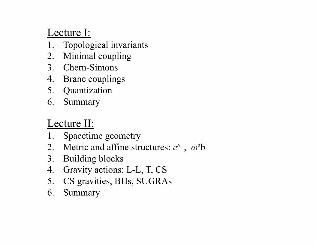
Lecture I: 1.  Topological invariants 2.  Minimal coupling 3.  Chern-Simons 4.  Brane couplings 5.  Quantization 6.  Summary

Lecture II: 1.  Spacetime geometry 2.  Metric and affine structures: ea , ωab 3.  Building blocks 4.  Gravity actions: L-L, T, CS 5.  CS gravities, BHs, SUGRAs 6.  Summary

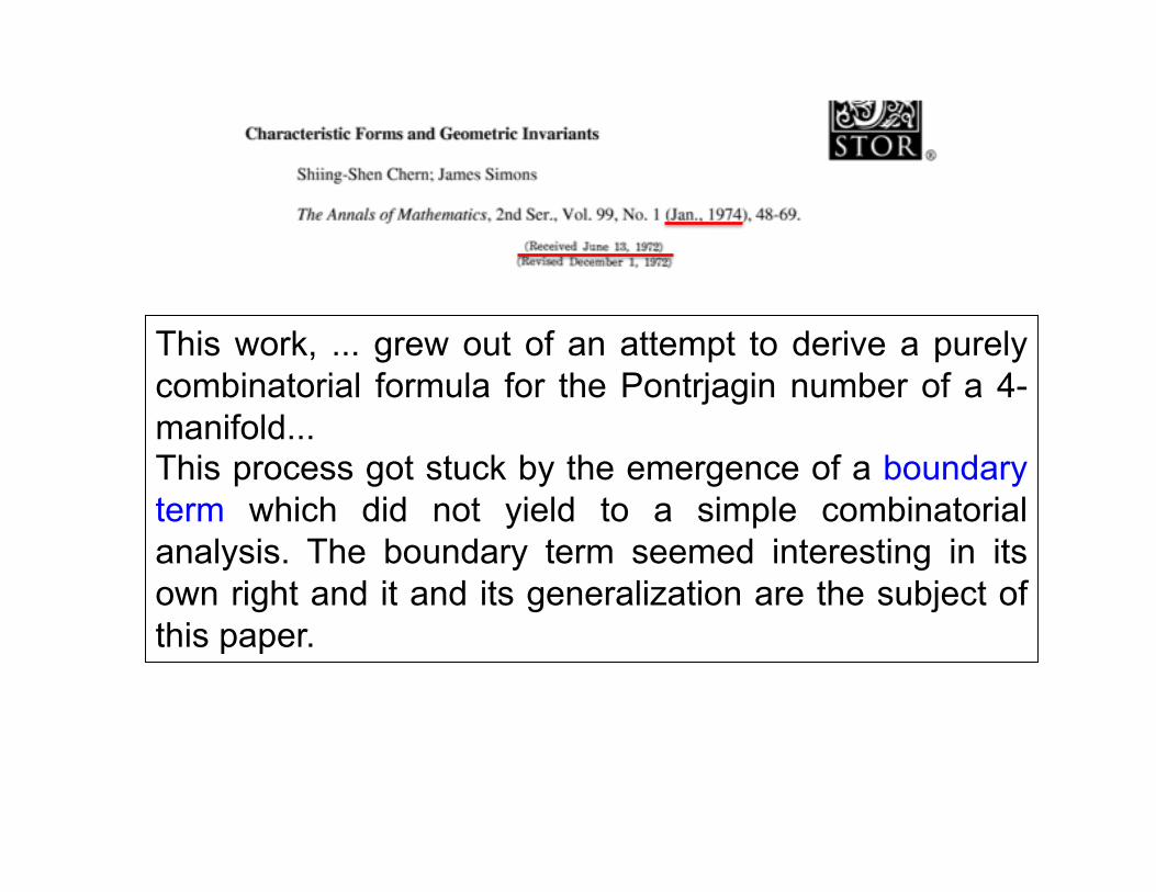
This work, ... grew out of an attempt to derive a purely combinatorial formula for the Pontrjagin number of a 4-manifold... This process got stuck by the emergence of a boundary term which did not yield to a simple combinatorial analysis. The boundary term seemed interesting in its own right and it and its generalization are the subject of this paper.

1. Topological invariants

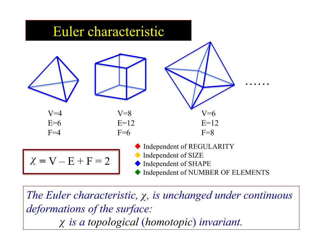
Euler characteristic

V=4 E=6 F=4

V=8 E=12 F=6

V=6 E=12 F=8

……

  Independent of REGULARITY   Independent of SIZE   Independent of SHAPE   Independent of NUMBER OF ELEMENTS

= V – E + F = 2 χ

The Euler characteristic, , is unchanged under continuous deformations of the surface:

is a topological (homotopic) invariant.

χ

χ

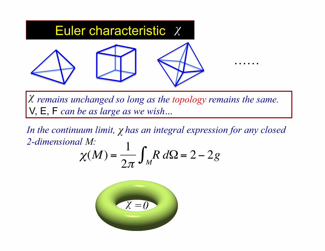
Euler characteristic

……

remains unchanged so long as the topology remains the same. V, E, F can be as large as we wish... χ

In the continuum limit, has an integral expression for any closed 2-dimensional M:

χ

€

χ(M ) =1

2π RM∫ dΩ= 2− 2g

χ

χ =0

The Euler characteristic belongs to a family of famous invariants:

All of these examples involve topological invariants called the Chern characteristic classes and Chern-Simons forms.

  Sum of exterior angles of a polygon   Residue theorem in complex analysis   Winding number of a map   Poincaré-Hopff theorem (“one cannot comb a sphere”)   Atiyah-Singer index theorem   Witten index   Dirac’s monopole quantization   Aharonov-Bohm effect   Gauss’ law   Bohr-Sommerfeld quantization   Soliton/Instanton topologically conserved charges   etc…

2. Minimal coupling

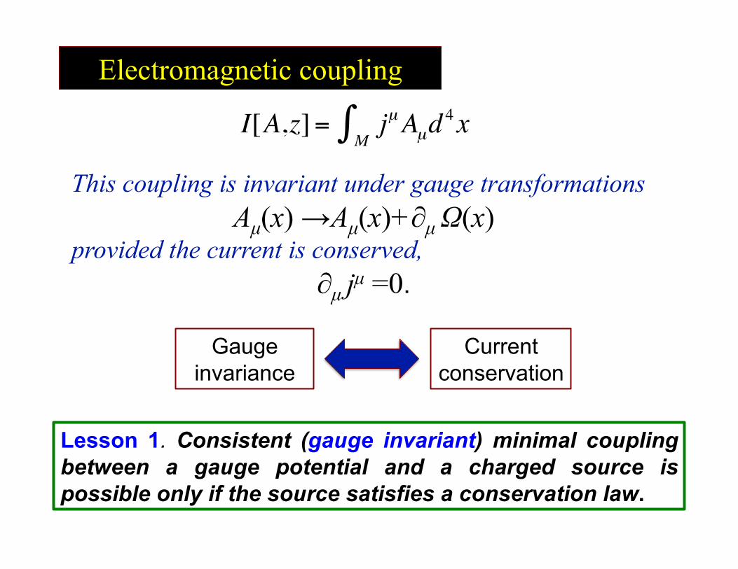
This coupling is invariant under gauge transformations Aµ(x) →Aµ(x)+∂µ Ω(x)

provided the current is conserved, ∂µ jµ =0.

€

I[A,z]= jµAµM∫ d 4x

Electromagnetic coupling

Gaugeinvariance

Current conservation

Lesson 1. Consistent (gauge invariant) minimal coupling between a gauge potential and a charged source is possible only if the source satisfies a conservation law.

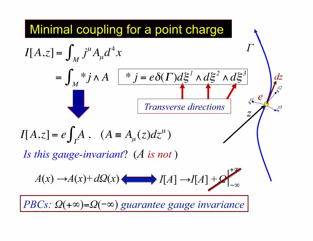
Minimal coupling for a point charge

€

I[A,z]= jµAµM∫ d 4x

Is this gauge-invariant? (A is not )

€

= * j∧AM∫

€

* j = eδ(Γ )dξ 1 ∧dξ 2 ∧dξ 3

Transverse directions

ξ2

ξ1

ξ3 z

e

Γ

dz

A(x) →A(x)+dΩ(x) I[A] →I[A] +Ω| -∞ +∞

PBCs: Ω(+∞)=Ω(-∞) guarantee gauge invariance €

I[A,z] = e AΓ∫ , (A ≡ Aµ (z)dzµ )

€

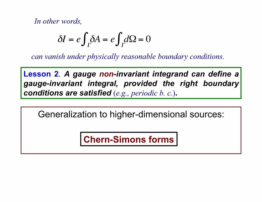
δI = e δAΓ∫ = e dΩ

Γ∫ = 0

In other words,

can vanish under physically reasonable boundary conditions.

Lesson 2. A gauge non-invariant integrand can define a gauge-invariant integral, provided the right boundary conditions are satisfied (e.g., periodic b. c.).

Generalization to higher-dimensional sources:

Chern-Simons forms

3. Chern-Simons forms

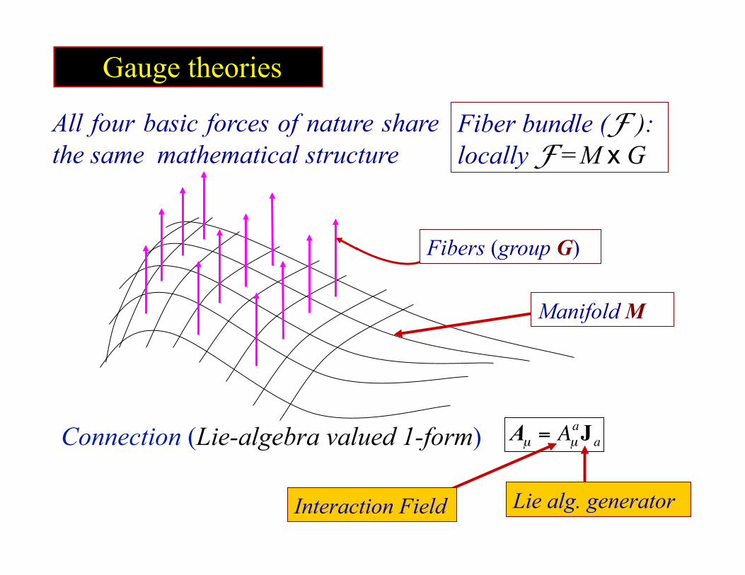
All four basic forces of nature share the same mathematical structure

Fiber bundle (F ): locally F =M x G

Gauge theories

Fibers (group G)

Connection (Lie-algebra valued 1-form)

€

Aµ = AµaJa

Lie alg. generator Interaction Field

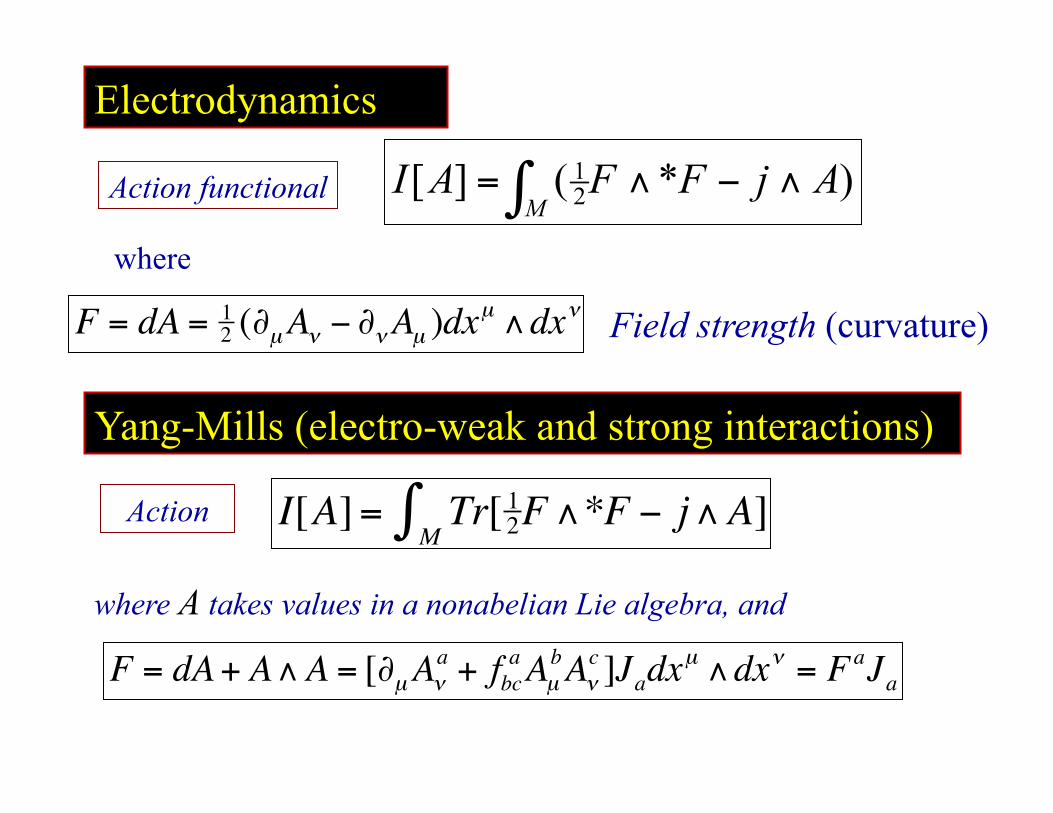
Electrodynamics

€

F = dA = 12 (∂µAν − ∂νAµ )dx

µ ∧dxνwhere

Field strength (curvature)

Action functional

Yang-Mills (electro-weak and strong interactions)

Action

€

I[A]= Tr[ 12M∫ F∧*F − j∧A]

where A takes values in a nonabelian Lie algebra, and

€

F = dA+ A∧A = [∂µAνa + fbc

a AµbAν

c ]Jadxµ ∧dxν = FaJa

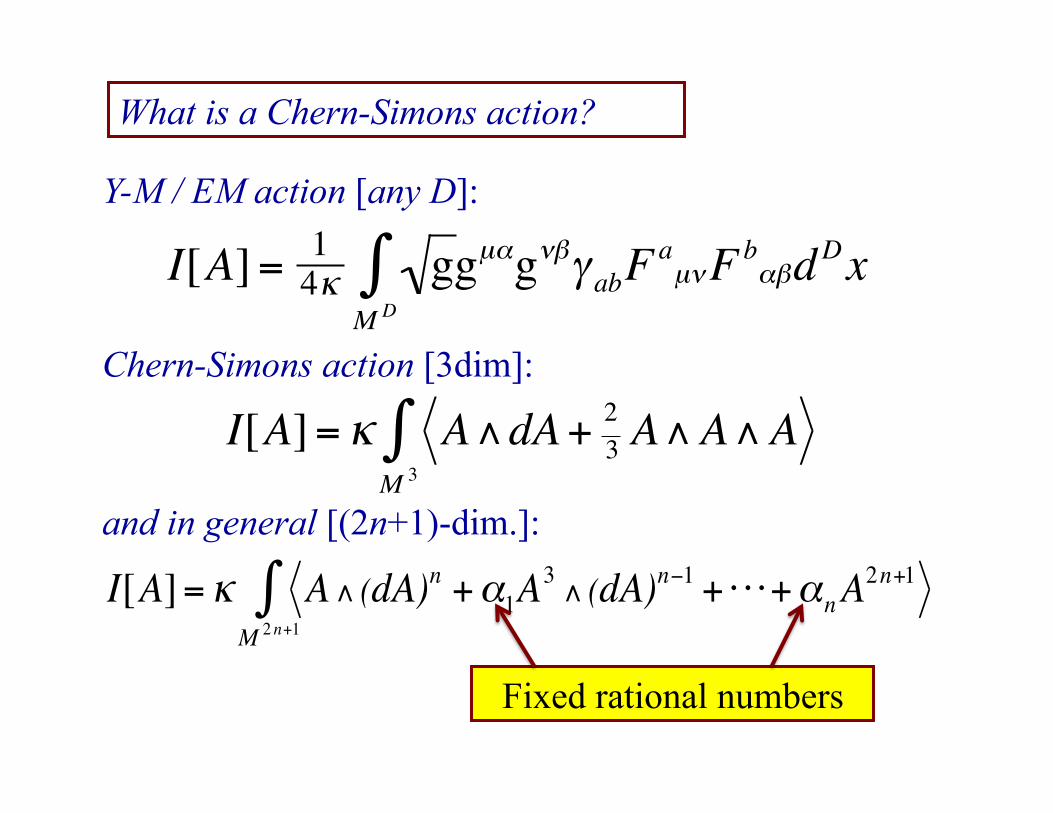
What is a Chern-Simons action?

€

I[A]= 14κ ggµαgνβγ abF

aµνFb

αβ

M D∫ dDx

Y-M / EM action [any D]:

€

I[A]= κ A∧dA+ 23 A∧A∧A

M 3∫

Chern-Simons action [3dim]:

€

I[A]= κ A∧ (dA)n +α1A3 ∧ (dA)n−1 + ⋅ ⋅ ⋅+αnA

2n+1

M 2 n+1∫

and in general [(2n+1)-dim.]:

Fixed rational numbers

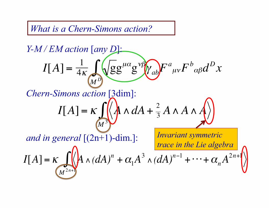
What is a Chern-Simons action?

€

I[A]= 14κ ggµαgνβγ abF

aµνFb

αβ

M D∫ dDx

€

I[A]= κ A∧dA+ 23 A∧A∧A

M 3∫

Chern-Simons action [3dim]:

€

I[A]= κ A∧ (dA)n +α1A3 ∧ (dA)n−1 + ⋅ ⋅ ⋅+αnA

2n+1

M 2n+1∫

and in general [(2n+1)-dim.]: Invariant symmetric trace in the Lie algebra

Y-M / EM action [any D]:

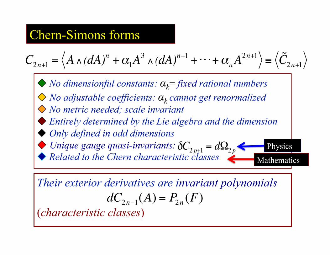
Their exterior derivatives are invariant polynomials

(characteristic classes)

€

dC2n−1(A) = P2n (F)

Chern-Simons forms

No dimensionful constants: αk= fixed rational numbers

No adjustable coefficients: αk cannot get renormalized No metric needed; scale invariant Entirely determined by the Lie algebra and the dimension

  Only defined in odd dimensions Unique gauge quasi-invariants: Related to the Chern characteristic classes

€

C2n+1 = A∧ (dA)n +α1A3 ∧ (dA)n−1 + ⋅ ⋅ ⋅+αn A2n+1 ≡ ˜ C 2n+1

€

δC2 p+1 = dΩ2 p Physics

Mathematics

the polynomial is invariant

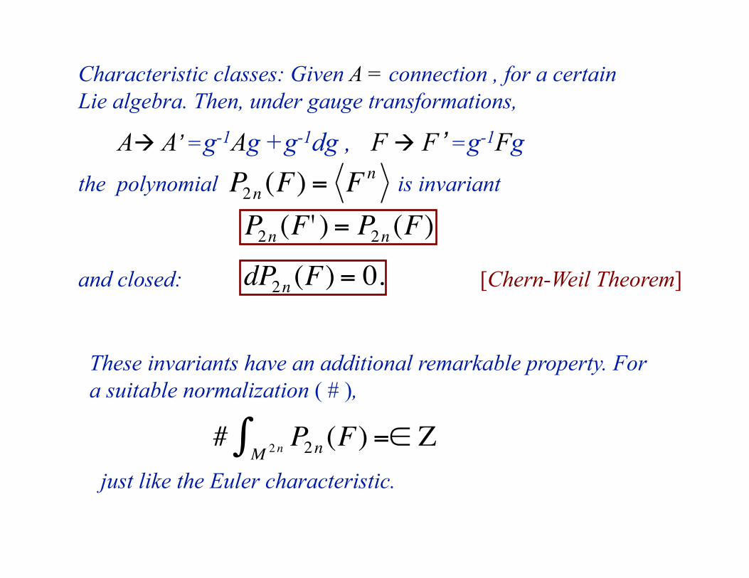
Characteristic classes: Given A = connection , for a certain Lie algebra. Then, under gauge transformations,

€

P2n (F) = FnA A’ =g-1Ag +g-1dg , F F ’ =g-1Fg

These invariants have an additional remarkable property. For a suitable normalization ( # ),

just like the Euler characteristic.

€

# P2n (F)M 2n∫ =∈ Z

€

P2n (F' ) = P2n (F)

and closed: [Chern-Weil Theorem]

€

dP2n (F) = 0.

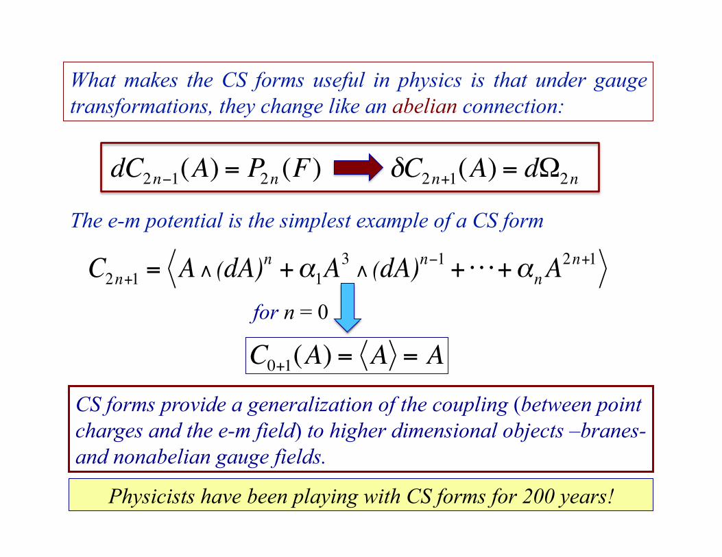
What makes the CS forms useful in physics is that under gauge transformations, they change like an abelian connection:

CS forms provide a generalization of the coupling (between point charges and the e-m field) to higher dimensional objects –branes- and nonabelian gauge fields.

The e-m potential is the simplest example of a CS form

€

C0+1(A) = A = A

€

δC2n+1(A) = dΩ2n

€

dC2n−1(A) = P2n (F)

€

C2n+1 = A∧ (dA)n +α1A3 ∧ (dA)n−1 + ⋅ ⋅ ⋅+αnA

2n+1

for n = 0

Physicists have been playing with CS forms for 200 years!

€

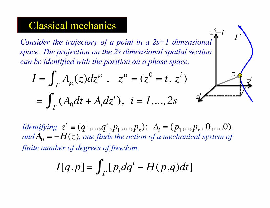
I = AµΓ∫ (z)dzµ , zµ = (z0 = t, zi )

Classical mechanics Consider the trajectory of a point in a 2s+1 dimensional space. The projection on the 2s dimensional spatial section can be identified with the position on a phase space.

€

= (A0Γ∫ dt + Aidz

i ), i = 1,..., 2s

z

Γ z0=t

zi

zj

Identifying , and , one finds the action of a mechanical system of finite number of degrees of freedom,

€

zi ≡ (q1,...,qs, p1,..., ps); Ai = (p1,.., ps , 0,...,0)

€

A0 = −H (z)

€

I[q, p]= [pidqi −H (p,q)dt]

Γ∫

€

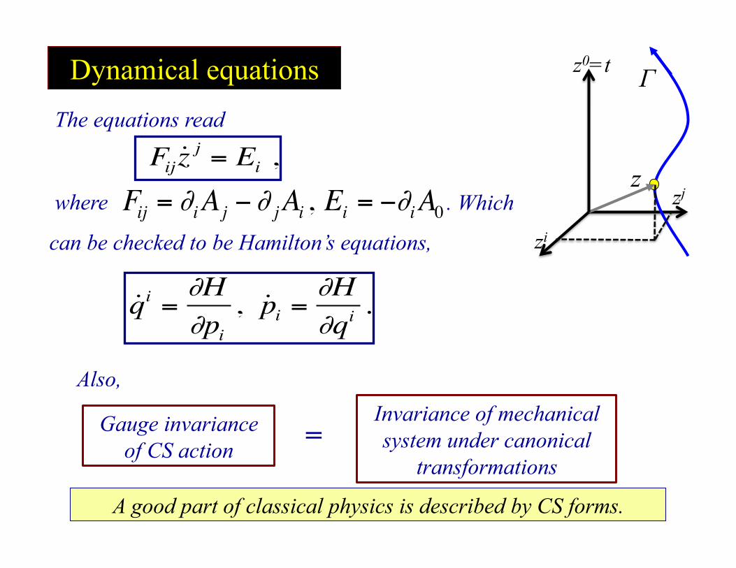
Fij ˙ z j = Ei ,

Dynamical equations The equations read

€

Fij = ∂iAj −∂ jAi , Ei = −∂iA0where . Which

can be checked to be Hamilton’s equations,

z

Γ z0=t

zi

zj

= €

˙ q i =∂H∂pi

, ˙ p i =∂H∂qi .

Gauge invariance of CS action

Invariance of mechanical system under canonical

transformations

Also,

A good part of classical physics is described by CS forms.

4. Chern-Simons couplings

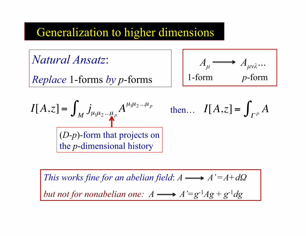
Generalization to higher dimensions

Natural Ansatz: Replace 1-forms by p-forms

(D-p)-form that projects on the p-dimensional history

Aµ Aµνλ… 1-form p-form

This works fine for an abelian field: A A’ =A+dΩ

but not for nonabelian one: A A’=g-1Ag + g-1dg

then…

€

I[A,z]= AΓ p∫

€

I[A,z]= jµ1µ2 ...µ pAµ1µ2 ...µ p

M∫

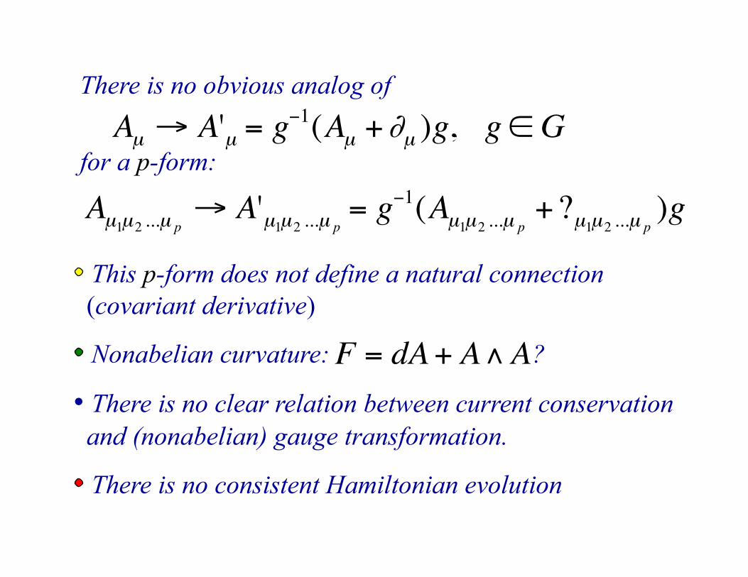
There is no obvious analog of

for a p-form:

€

Aµ → A'µ = g−1(Aµ +∂µ )g, g∈G

€

Aµ1µ2 ...µ p→ A'µ1µ2 ...µ p

= g−1(Aµ1µ2 ...µ p+?µ1µ2 ...µ p

)g

This p-form does not define a natural connection (covariant derivative)

Nonabelian curvature: ?

•  There is no clear relation between current conservation and (nonabelian) gauge transformation.

There is no consistent Hamiltonian evolution €

F = dA+ A∧A

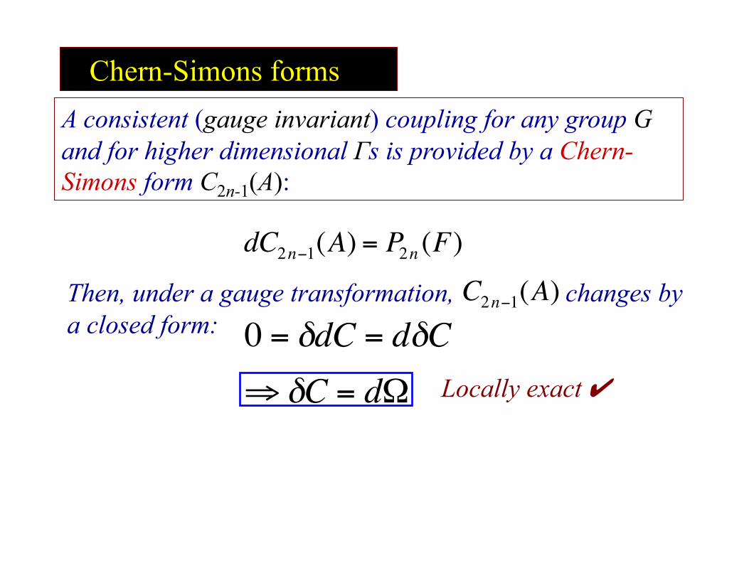
A consistent (gauge invariant) coupling for any group G and for higher dimensional Γs is provided by a Chern-Simons form C2n-1(A):

Chern-Simons forms

€

⇒δC = dΩ Locally exact ✔

Then, under a gauge transformation, changes by a closed form:

€

C2n−1(A)

€

dC2n−1(A) = P2n (F)

€

0 = δdC = dδC

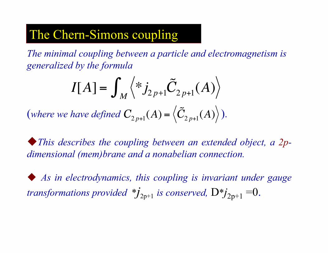
The minimal coupling between a particle and electromagnetism is generalized by the formula

(where we have defined ).

The Chern-Simons coupling

€

I[A] = * j2 p+1˜ C 2 p+1(A)

M∫

  As in electrodynamics, this coupling is invariant under gauge transformations provided *j2p+1 is conserved, D*j2p+1 =0.

 This describes the coupling between an extended object, a 2p-dimensional (mem)brane and a nonabelian connection.

€

C2 p+1(A) = ˜ C 2 p+1(A)

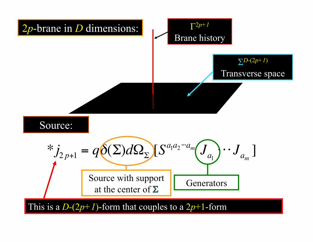
2p-brane in D dimensions:

€

* j2 p+1 = qδ(Σ)dΩΣ [Sa1a2 ⋅⋅⋅am Ja1

⋅ ⋅ ⋅ Jam ]

Source:

This is a D-(2p+1)-form that couples to a 2p+1-form

Source with support at the center of

Generators

Γ2p+1

Brane history

ΣD-(2p+1)

Transverse space

The Chern-Simons coupling

€

I[A] = * j2 p+1˜ C 2 p+1(A)

M∫ ,Lemma:

Proof: This can be explicitly verified. //

is invariant under gauge transformations, provided j2p+1 is conserved, d*j2p+1 + [A, *j2p+1]=D*j2p+1 = 0.

N.B.: If the current is produced by particles or fields that are dynamically governed by an action principle, invariant under the same gauge symmetry, then Noether theorem guarantees that such conserved current can always be explicitly written out. //

5. Examples of branes

•  An m-brane is a localized (m+1)-dimensional manifold, embedded in spacetime.

•  They disrupt the homogeneity of spacetime (impurities)

•  They are obstructions that change the topology of spacetime(topological defects)

•  Examples: point particle (m=0), domain wall (m=2),

2p-brane (m=2p)

Γ

Branes are defects

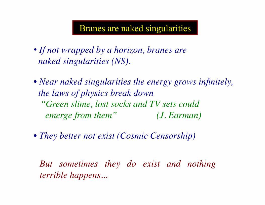
•  If not wrapped by a horizon, branes are naked singularities (NS).

•  Near naked singularities the energy grows infinitely, the laws of physics break down “Green slime, lost socks and TV sets could emerge from them” (J. Earman)

•  They better not exist (Cosmic Censorship)

Branes are naked singularities

But sometimes they do exist and nothing terrible happens...

0-brane [point charge]:

€

* j = eδ(Γ)dΩD−1

0- and 2- brane sources in EM (4D)

€

↔ jµ = e˙ z µδ(3)( x − z )dτ ✔

2-brane [interface between two regions in 3-space]:

€

* j = −θδ(Σ)dn

€

↔ jµνλ = −θεµνλ⊥δ(x⊥ )d 3x(Σ)

n θin≠0

This brane is the 2D surface Σ of a solid volume in 3D, whose history is a 2+1 worldsheet .

θout=0

€

Σ×R

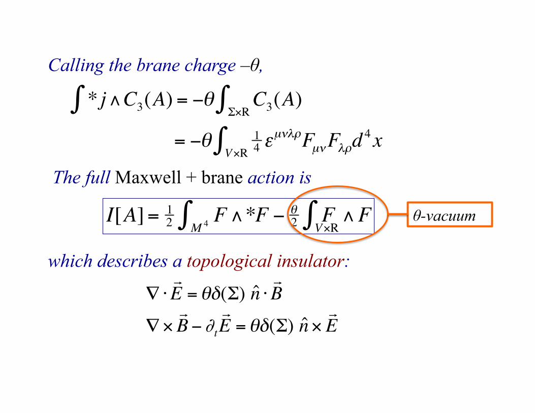
Calling the brane charge –θ,

The full Maxwell + brane action is

which describes a topological insulator: €

* j∧C3(A)∫ = −θ C3(A)Σ×R∫

= −θ 14 ε

µνλρFµνV×R∫ Fλρd4x

€

I[A]= 12 F∧*F

M 4∫ − θ2 F

V×R∫ ∧F

€

∇ ⋅ E =θδ(Σ) ˆ n ⋅

B

∇× B −∂t

E =θδ(Σ) ˆ n ×

E

θ-vacuum

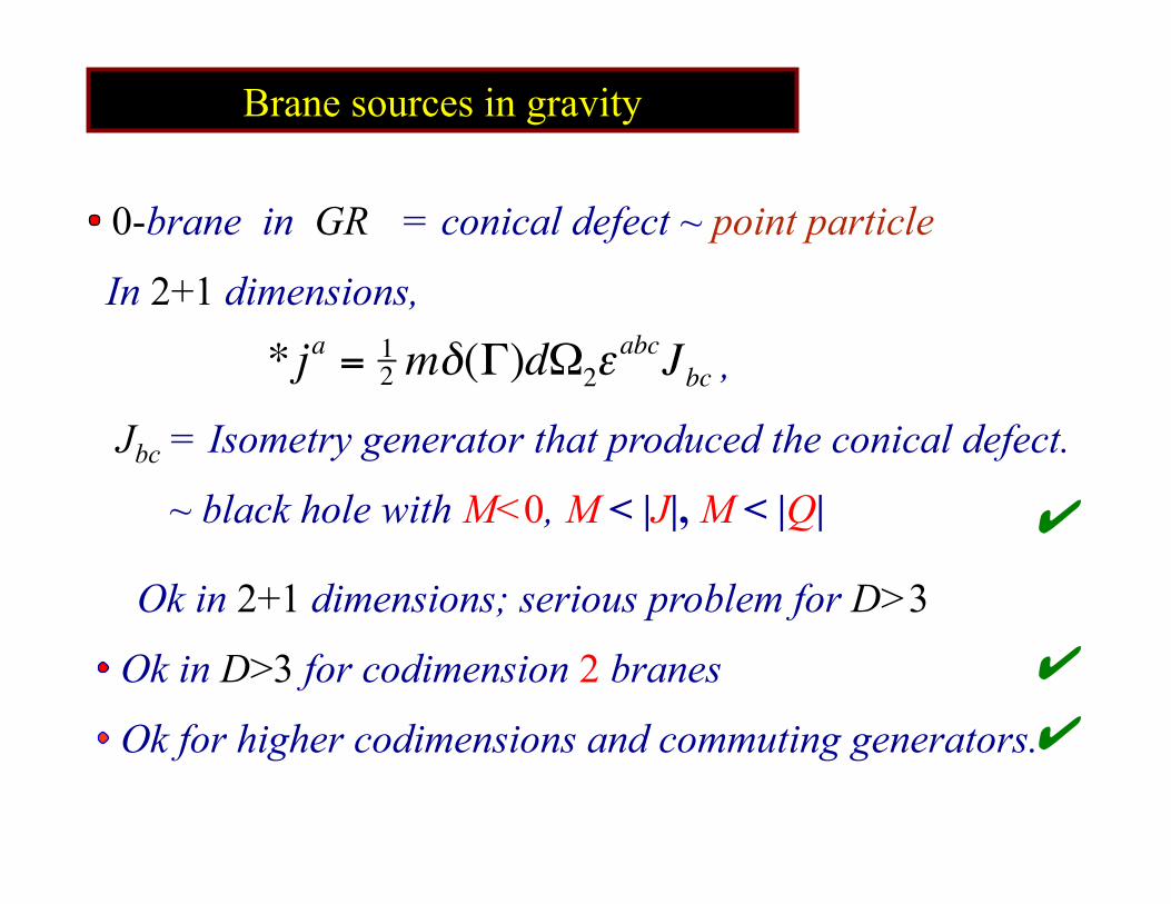
0-brane in GR = conical defect ~ point particle

Brane sources in gravity

€

* ja = 12 mδ(Γ)dΩ2ε

abcJbc

In 2+1 dimensions,

,

Jbc = Isometry generator that produced the conical defect.

~ black hole with M<0, M < |J|, M < |Q| ✔

Ok in 2+1 dimensions; serious problem for D>3

Ok in D>3 for codimension 2 branes

Ok for higher codimensions and commuting generators. ✔

✔

6. Quantization

€

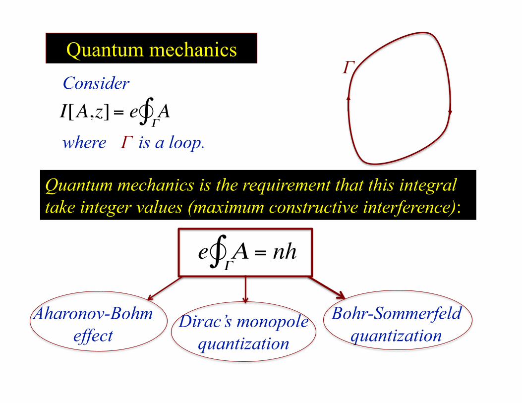
I[A,z]= e AΓ∫

Quantum mechanics Consider

where is a loop. Γ

Γ

Quantum mechanics is the requirement that this integral take integer values (maximum constructive interference):

€

e ΑΓ∫ = nh

Dirac’s monopole quantization

Aharonov-Bohm effect

Bohr-Sommerfeld quantization

€

AΓ∫ = AµΓ

∫ (z)dzµ , zµ = (z0 = t, zi )

Bohr-Sommerfeld quantization Consider a mechanical system described by a CS lagrangian in a 2s+1 dimensional space.

€

= (A0Γ∫ dt + Aidz

i ), i = 1,..., 2s

If the orbit is periodic, one finds the B-S quantization condition

€

AΓ∫ = [pidq

iΓ∫ −H (p,q)dt]

€

= 2nπ = nh

Γ

€

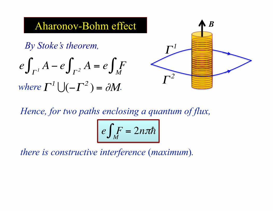
e AΓ 1∫ − e A

Γ 2∫ = e FM∫

Aharonov-Bohm effect

By Stoke’s theorem,

where .

€

Γ 1 (−Γ 2 ) = ∂M

Hence, for two paths enclosing a quantum of flux,

B

€

Γ 2

€

Γ 1

€

e FM∫ = 2nπ

there is constructive interference (maximum).

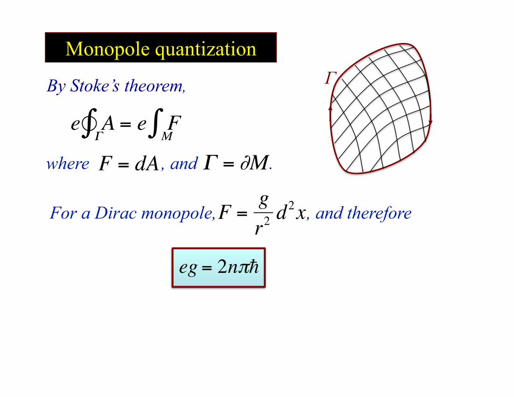
Monopole quantization Γ

€

e AΓ∫ = e F

M∫By Stoke’s theorem,

where , and .

€

Γ = ∂M

€

F = dA

For a Dirac monopole, , and therefore

€

F =gr2d2x

€

eg = 2nπ

7. Summary

Summary

•  CS forms generalize the coupling between a point charge and the electromagnetic field, providing a natural gauge-invariant way to couple gauge fields (abelian or not) to extended sources: 2p-branes.

•  The simplest CS action can also describe an arbitrary classical mechanical system of finite degrees of freedom.

•  Path integral quantization yields the Bohr-Sommerfeld quantum postulate, Dirac’s monopole quantization and the Aharonov-Bohm effect.

•  Mathematically, CS forms are related to topological invariants, the Chern characteristic classes.

Bibliography

Shiing-Shen Chern and James Simon: Characteristic Forms and Geometric Invariants, Ann. Math. 99 (1974) 48.

J.Z.: Lecture Notes on Chern-Simons (Super-)Gravities [Second Edition] arXiv: hep-th/0502193v4.

J.Z.: Uses of Chern-Simons Forms, (In 10 Years of the AdS/CFT Conjecture), arXiv: hep-th/0805.1778

J.Z.: Chern-Simons Forms in Gravitation Theories, Class. & Quant. Grav. 29 (2012) 133001.

J.Z.: Gravitation Theory and Chern-Simons Forms, Villa de Leyva School, 2011.

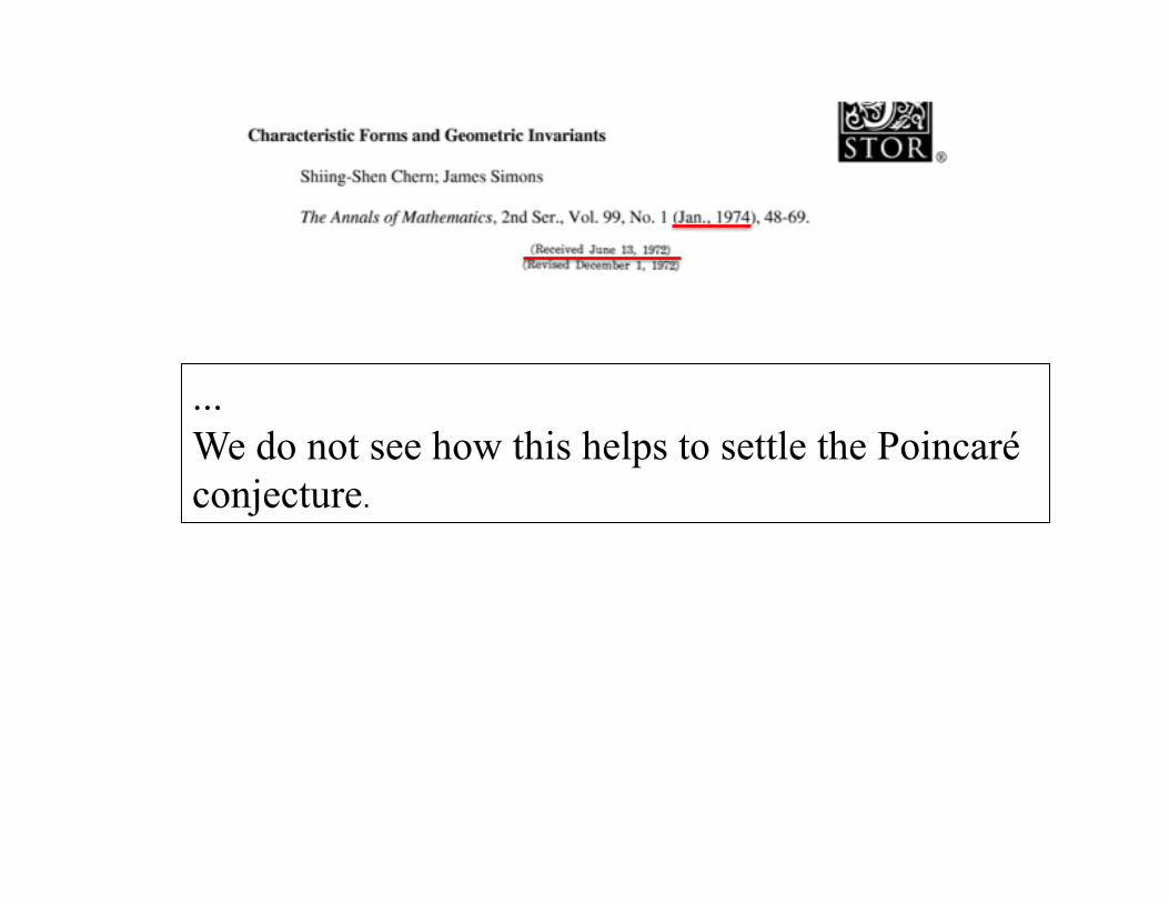
... We do not see how this helps to settle the Poincaré conjecture.