Introduction to Business Statistics Chapter 7 Spring 2008 7-2.pdfPopulation and sampling...

QM-120, M. Zainal

DEPARTMENT OF QUANTITATIVE METHODS & INFORMATION SYSTEMS

Introduction to Business StatisticsQMIS 220Chapter 7

Dr. Mohammad ZainalSpring 2008

QMIS 220, CH 7 by M. Zainal

2

The Normal distribution

A large number of real world phenomena are either exactly or approximately normally distributed and that leads to make the normal distribution to be the most important and widely used one.

The normal distribution or Gaussian distribution is given by a bell‐shaped curve.

A continuous RV x that has a normal distribution is said to be a normal RV with a mean µ and a standard deviation σ or simply x~N(µ,σ).

The mean µ and the standard deviation σ are the parameters of the normal distribution.

Given the values of these two parameters, we can find the area under the normal curve for any interval.

QM-120, M. Zainal


3


The normal probability distribution, when plotted, gives a bell‐shaped curve such that

The total area under the curve is 1.0.The curve is symmetric around the mean.The two tails of the curve extended indefinitely.


4


There are a family of normal distribution.Each different set of values of µ and σ gives different normal

curve.The value of µ determines the center of the curve on the

horizontal axis and the value of σ gives the spread of the normal curve

QM-120, M. Zainal


5


Like all other distributions, the normal probability distribution can be expressed by a mathematical function

in which the probability that x falls between a and b is the integral of the above function from a to b, i.e.

2121( )

2

xb

a

P a x b e dxµ

σ

σ π

−⎡ ⎤− ⎢ ⎥⎣ ⎦< < = ∫

2121( )

2

x

f x eµ

σ

σ π

−⎡ ⎤− ⎢ ⎥⎣ ⎦=


6


But as you know, we will not use the formula to find the probability. instead, we will use a table.

QM-120, M. Zainal


7


The standard normal distribution is a special case of the normal distribution where the µ is zero and the σ is 1.

The RV that possesses the standard normal distribution is denoted by z and it is called z values or z scores.

-4 -2 0 2 4z

µ=0

σ=1


8


Since µ is zero and the σ is 1 for the standard normal, a specific value of z gives the distance between the mean and the point represented by z in terms of the standard deviation.

The z values to the right side of the mean are positive and those on the left are negative BUT the area under the curve is always positive.

For a value of z = 2, we are 2 standard deviations from the mean (to the right).

Similarly, for z = ‐2, we are 2 standard deviations from the mean (to the left)

QM-120, M. Zainal


9



10


Empirical rule

QM-120, M. Zainal


11


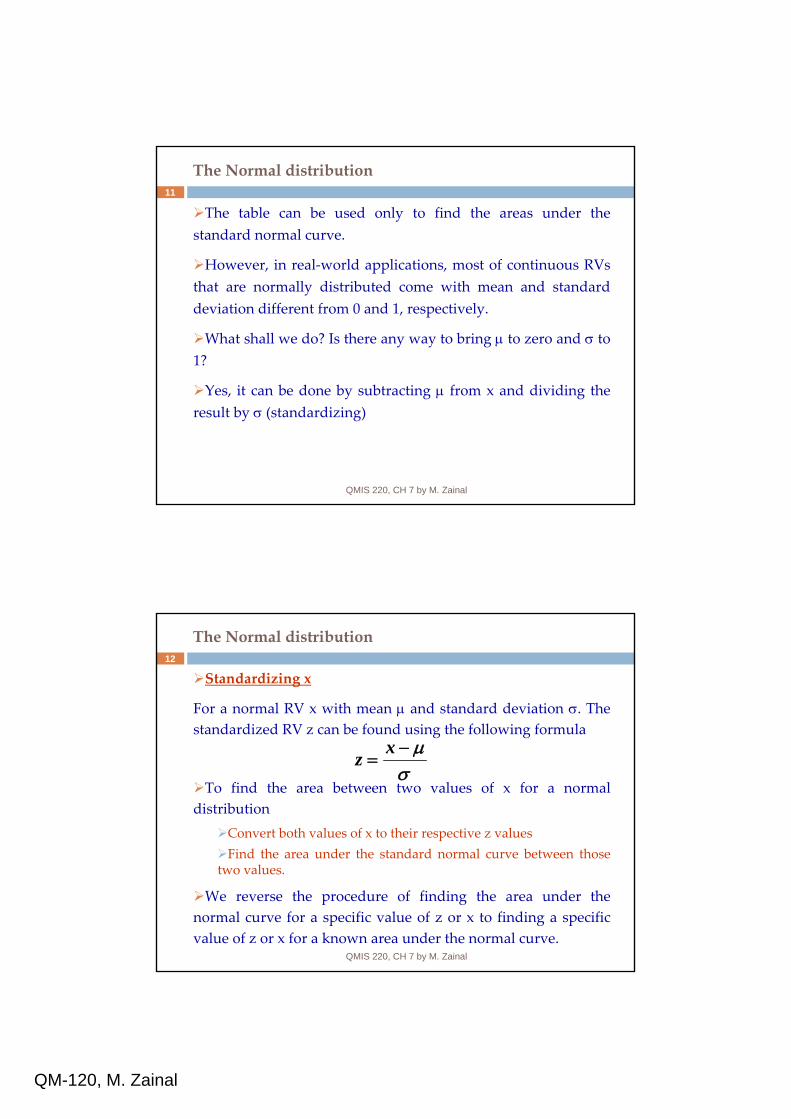
The table can be used only to find the areas under the standard normal curve.

However, in real‐world applications, most of continuous RVs that are normally distributed come with mean and standard deviation different from 0 and 1, respectively.

What shall we do? Is there any way to bring µ to zero and σ to 1?

Yes, it can be done by subtracting µ from x and dividing the result by σ (standardizing)


12


Standardizing x

For a normal RV x with mean µ and standard deviation σ. The standardized RV z can be found using the following formula

To find the area between two values of x for a normal distribution

Convert both values of x to their respective z valuesFind the area under the standard normal curve between those

two values.

We reverse the procedure of finding the area under the normal curve for a specific value of z or x to finding a specific value of z or x for a known area under the normal curve.

xz µσ−

=

QM-120, M. Zainal


13


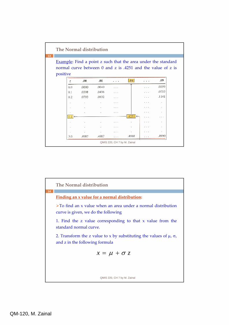
Example: Find a point z such that the area under the standard normal curve between 0 and z is .4251 and the value of z is positive


14


Finding an x value for a normal distribution:

To find an x value when an area under a normal distribution curve is given, we do the following

1. Find the z value corresponding to that x value from the standard normal curve.

2. Transform the z value to x by substituting the values of µ, σ, and z in the following formula

x zµ σ= +

QM-120, M. Zainal


15

Population and sampling distribution

Random Sampling:

The term random sampling refers to a sampling procedure where every member in the population has a chance of being selected.

The objective of the sampling procedure is to ensure that the final sample is representative of the population from which it was taken

A biased sample is a sample that doesn’t represent the intended population and can lead to distorted findings.


16


Simple Random Sampling (SRS):

A simple random sample is a sample in which every member of the population has an equal chance of being selected.

Unfortunately, this is easier said than done!

Using a random numbers table we can start randomly selecting our elements.

QM-120, M. Zainal


17


If we want to conduct a survey in a mall using SRS.

Depending on the population size, we can choose the 1st digits from each random number.

Suppose the were 1000 shoppers in the mall, from which we were drawing a sample size of 100.

We would list these shoppers with the assigned number: 24, 19, 46, 17, 22, 93, 52, 62….and so forth.


18


Systematic Sampling:

One way to avoid a personal bias when selecting people at random is to use symmetric sampling.

This technique results in selecting every kth member of the population to be in the sample.

K ≈ N / n, where N is the population size and n is the sample size.

Much easier and cheaper to conduct.

Very dangerous if there is a pattern in the population

QM-120, M. Zainal


19


Cluster Sampling:

If the population can be divided into groups, or clusters, then simple random sample can be selected from these clusters to form the final sample.

These clusters could be classes in a school or stores in a mall.

Once the cluster is selected, all the elements inside that cluster must be included in the sample


20


Stratified Sampling:

In stratified sampling, we divide the population into mutually exclusive groups, or strata, and randomly sample from each of these groups.

Using our mall example, our strata could be defined as male and female shoppers.

We can be sure that our final sample contains a number of male and female shoppers with the same proportion in the population.

Other examples of stratus: age, income, occupation.

QM-120, M. Zainal


21


Sampling Error:

So far, we have stressed the benefits of drawing a sample from a population.

However, in statistics, as in life, thereʹs no such thing as a free lunch.

By sampling, we expose ourselves to errors that can lead to inaccurate conclusions about the population.

The type of error that a statistician is most concerned about iscalled sampling error, which occurs when the sample measurement is different from the population measurement.


22


Because the entire population is rarely measured, the sampling error cannot be directly calculated.

However, with inferential statistics, weʹll be able to assign probabilities to certain amounts of sampling error later.

Sampling errors occur because we might have the unfortunate luck of selecting a sample that is not a perfect match to the entire population.

Sampling errors are expected and usually are a small price to pay to avoid measuring an entire population.

One way to reduce the sampling error of a statistical study is to increase the size of the sample.

QM-120, M. Zainal


23


In general, the larger the sample size, the smaller the samplingerror.

If you increase the sample size until it reaches the size of thepopulation, then the sampling error will be reduced to 0.

But in doing so, we lose the benefits of sampling.


24


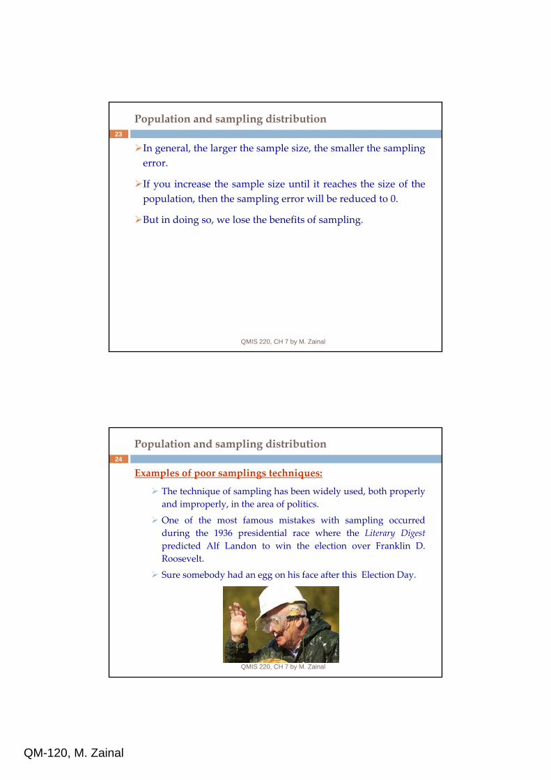
Examples of poor samplings techniques:

The technique of sampling has been widely used, both properly and improperly, in the area of politics.

One of the most famous mistakes with sampling occurred during the 1936 presidential race where the Literary Digest predicted Alf Landon to win the election over Franklin D. Roosevelt.

Sure somebody had an egg on his face after this Election Day.

QM-120, M. Zainal


25


Population distribution:

The population distribution is the probability distribution derived form the information on all elements of a population.

Example:

Suppose there are only five students in a MBA class and the midterm scores of these five students are.

Name Score

A 70

B 78

C 80

D 80

E 95


26


The population frequency and relative frequency distributions table of the scores is:

The values of the mean and the standard deviation calculated for the probability distribution above give µ = 80.60 and σ = 8.09 (How & Why?)

Are these values constant?

x f R.f. P(x)

70 1 0.20 0.20

78 1 0.20 0.20

80 2 0.40 0.40

95 1 0.20 0.20

N = 5 Sum = 1.00 ΣP(x) = 1.00

QM-120, M. Zainal


27


Sampling distribution:

Suppose we want to draw a sample (without replacement) of three students from that class and see how much is their mean and standard deviation.

In this case, we will have 10 different samples.

ABC, ABD, ABE, ACD, ACE, ADE, BCD, BCE, BDE, CDE

Can you tell how ?

Each sample will have different mean and standard deviation depending on the elements included in the sample.


28


Sample Scores x Frequency and relative frequency distributions

Sampling distribution of x for n = 3ABC 70, 78, 80 76.00

ABD 70, 78, 80 76.00 x f R.f x P(x)

ABE 70, 78, 95 81.00 76.00 2 0.20 76.00 0.20

ACD 70, 80, 80 76.67 76.67 1 0.10 76.67 0.10

ACE 70, 80, 95 81.67 79.33 1 0.10 79.33 0.10

ADE 70, 80, 95 81.67 81.00 1 0.10 81.00 0.10

BCD 78, 80, 80 79.33 81.67 2 0.20 81.67 0.20

BCE 78, 80, 95 84.33 84.33 2 0.20 84.33 0.20

BDE 78, 80, 95 84.33 85.00 1 0.10 85.00 0.10

CDE 80, 80, 95 85.00 Σf =10 Sum = 1.00 ΣP(x)=1.00

QM-120, M. Zainal


29

Sampling and nonsampling errors

Sampling errors:

The difference between the sample mean (statistic) and the population mean (parameter) is called sampling error.

This difference is only due the chance of including some elements and excluding others in the random sample only.

Nonsampling errors:

The error that occur in the collection, recording, and tabulation of data are called nonsampling errors

µ−= x error Sampling

xx correctIncorrect error gNonsamplin −=


30

Sampling and nonsampling errors

Example:

Reconsider the population of the five scores. Suppose one sample of three scores is selected, and the sample is 70, 80, and 95.

1.Find the sampling error

2.Suppose we mistakenly record the second score as 82 instead of 80. Find the nonsampling error

QM-120, M. Zainal


31

Mean and standard deviation of x

If we calculate the mean and the standard deviation of all possible samples (with the same size n) mean and standarddeviations, we obtain the mean and the standard deviation vvvof .

The mean of the sampling distribution of is always equal to the mean of the population. Thus,

The sample mean is an estimator of the population mean and if they are equal, the statistic is said to be say it is unbiased estimator.

xµ

xxσ

x

µµ =x


32


The standard deviation , of is not equal to the standard deviation, , of the population distribution (unless n= 1)

To find the standard deviation of we use:

xxσ

x

⎪⎪⎩

⎪⎪⎨

⎧

−−

≤=

OtherwiseN

nNn

Nnif

nx

1

05.0

σ

σ

σ

σ

QM-120, M. Zainal


33


Example: The mean wage per hour for all 5000 employees who work at a large company is $17.50 and the standard deviation is $2.9. Let be the wage per hour for a random sample of certain employees selected from this company. Find the mean and the standard deviation of for a sample size of

a) 30 b) 75 c) 200

x

x


34


Example: The living spaces of all homes in a city have a mean of 2300 square feet and a standard deviation of 450 square feet.Let be the mean living space for a random sample of 25 homes selected from this city. Find the mean and the standard deviation of the sampling distribution x

x

QM-120, M. Zainal


35

Shape of the sampling distribution of x

The shape of the sampling distribution of depends on whether the population from which samples are drawn has a normal distribution or not.

Sampling from a normally distributed population

If the sample is drawn from a normally distributed population with a mean µ and a standard deviation σ, then the sampling distribution of will be normally distributed with the following mean and standard deviation, irrespective of the sample size:

x

x

nand xx

σσµµ ==


36


QM-120, M. Zainal


37


Sampling from a population that is not normally distributed

Central limit theorem (CLT) : For a large sample size, the sampling distribution of is approximately normal, irrespectiveof the shape of the population distribution.

The mean and standard deviation of are

30for n n

and xx ≥==σσµµ

x

x


38


QM-120, M. Zainal


39


Example: In a recent SAT, the mean score for all examinees was 1020. Assume that the distribution of SAT scores of all examinees is normal of 1020 and a standard deviation of 135. Let be the mean SAT score of a random sample of certain examinees. Calculate the mean and the standard deviation of jkj and describe the shape of its sampling distribution when the sample size is

a) 16 b) 50 c) 1000

x

x


40


Example: The weight of all people living in a town has a distribution that is skewed to the right with a mean of 133 pounds and a standard deviation of 24 pounds. Let be the mean weight of a random sample of 45 persons selected from this town. Find the mean and standard deviation of and comment on the shape of its sampling distribution.

x

x

QM-120, M. Zainal


41

Application of the sampling distribution of x

Based on the CLT, we can make the following statements:

6826.)11( =+≤≤− xx xP σµσµ 9544.)22( =+≤≤− xx xP σµσµ

9974.)33( =+≤≤− xx xP σµσµ


42


Example: Assume that the weights of all packages of a certain brand of cookies are normally distributed with a mean of 32 ounces and a standard deviation of .3 ounce. Find the probability that the mean weight, , of a random sample of 20packages of this brand of cookies will be between 31.8 and 31.9 ounces.

x

QM-120, M. Zainal


43


Example: The time that college students spend studying per week have a distribution that is skewed to the right with a mean 8.4 hours and a standard deviation of 2.7 hours. Find the probability that the mean time spent studying per week for a random sample of 45 students would be

a) Within 1 hour from the mean

b) Between 8 and 9 hours

c) Less than 8 hours


44

Population and sample proportion

What if we are dealing with qualitative variable?

Population proportion, denoted by p, is obtained by taking the ration of the number of elements in a population with a specific characteristic to the total number of elements in the population. It is calculated as

Sample proportion, denoted by (pronounced by p hat) gives a similar ratio for a sample and it is given by

NXp =

p̂

nxp =ˆ

QM-120, M. Zainal


45


Example: Suppose a total of 20,000 students are registered in KU for this semester and 14,500 of them own a laptop. A sample of 120 students is selected and 78 of them found to own a laptop. Find

a) the proportion of students who own a laptop in the population

b) the proportion of students who own a laptop in the sample

c) the sampling error


46


Sampling distribution of .

Like in the sample mean , the sample proportion is a random variable that possesses a probability distribution which is called its sampling distribution.

Remember that the probability distribution gives the various values that a RV may assume and their probabilities.

The value of for a particular sample depends on what elements of the population are included in that sample

p̂x

p̂

p̂

QM-120, M. Zainal


47


Mean, standard deviation, and shape of the sampling distribution of p

Example: The following table gives the names of the MBA students class along with their opinion of whether or not they like Statistics.

Name opinion

A yes

B no

C no

D yes

E yes


48



The population proportion is p = 3/5 = .60

The following table lists the 10 possible samples and the proportion of students who like statistics for each of those samples.

p̂

2/3 =.67CDE2/3 =.67ACE

2/3 =.67BDE2/3 =.67ACD

1/3 =.33BCE2/3 =.67ABE

1/3 = .33BCD2/3 =.67ABD

3/3 = 1.00ADE1/3 = .33ABC

SampleSample p̂

QM-120, M. Zainal


49



Frequency and relative frequency distributions Sampling distribution of x for n = 3

f R.f

.33 3 3/10 = .30 .33 0.30

.67 6 6/10 = .60 .67 0.60

1.00 1 1/10 = .10 1.00 0.10

Σf =10 Sum = 1.00 ΣP(x)=1.00

p̂ ˆ( )P pp̂


50



The mean of is always equal to the population proportion. That is

In which it is said to be unbiased estimator of the population proportion.

The standard deviation of is given byp̂

p̂

p̂ pµ =

ˆ

0.05

1

p

pq nifn Npq N n Otherwisen N

σ

⎧≤⎪⎪= ⎨

−⎪⎪ −⎩

QM-120, M. Zainal


51



According to the CLT, the shape of and the sampling distribution of will be approximately normal if

np > 5 and nq > 5

Example: The National survey of Student Engagement shows about 87% of freshmen and seniors rate their college experience as “good” or “excellent”. Let be the proportion of freshmen and seniors in a random sample of 900 who hold this view. Find the mean and the standard deviation of and describe the shape of its sampling distribution.

p̂

p̂

p̂

p̂


52


Applications of the sampling distribution of p

Example: According to a 2002 University of Michigan survey, only about one third of Americans expected the next five years to bring continuous good times. Assume that 33% of the current population of all Americans hold this opinion. Let be the proportion in a random sample of 800 Americans who will hold this opinion. Find the probability that the value of is between .35 and .37.

p̂

p̂

QM-120, M. Zainal


53


Applications of the sampling distribution of p

Example: Ahmad Ali, who was running for the parliament last summer, thinks that he is favored by 53% of all eligible voters in his district. Assume that what he think is true. What is the probability that in a random sample of 400 voters attended one of his campaign speeches, less than 49% will favor him.

Introduction to Business Statistics Chapter 7 Spring 2008 7-2.pdfPopulation and sampling...

Documents

Transcript of Introduction to Business Statistics Chapter 7 Spring 2008 7-2.pdfPopulation and sampling...